From least action in electrodynamics to magnetomechanical energy – a review

Abstract

The equations of motion for electromechanical systems are traced back to the fundamental Lagrangian of particles and electromagnetic fields, via the Darwin Lagrangian. When dissipative forces can be neglected the systems are conservative and one can study them in a Hamiltonian formalism. The central concepts of generalized capacitance and inductance coefficients are introduced and explained. The problem of gauge independence of self-inductance is considered. Our main interest is in magnetomechanics, i.e. the study of systems where there is exchange between mechanical and magnetic energy. This throws light on the concept of magnetic energy, which according to the literature has confusing and peculiar properties. We apply the theory to a few simple examples: the extension of a circular current loop, the force between parallel wires, interacting circular current loops, and the rail gun. These show that the Hamiltonian, phase space, form of magnetic energy has the usual property that an equilibrium configuration corresponds to an energy minimum.

1 Introduction

Electromagnetism is usually taught at the undergraduate level without mention of Lagrangians, Hamiltonians, or the principle of least action. In modern theoretical physics of gauge field theory, however, the concept of an invariant Lagrangian density has become the standard starting point. The Lagrangian formalism of analytical mechanics was introduced into electromagnetism already by Maxwell in his Treatise [1] who, using this approach, derives equations for electric circuits and for electromechanical systems. Since then its importance has kept growing. One can therefore argue that this set of tools should be better known and become accessible at an earlier stage in the physics curricula. This review attempts to be an aid in such efforts.

Our starting point is the basic Lagrangian density of classical electrodynamics as set down early in the last century by Larmor and Schwarzschild. From there we proceed to neglect radiation which leads us to the Darwin Lagrangian [2]. Then the path to classical linear circuit theory is traced. It is pointed out that the similarity between the Lagrangian formulation of mechanics and of circuit theory has deep physical reasons and is not just a formal similarity. In a long Appendix the generalized capacitance coefficients and the coefficients of self and mutual induction of circuit theory are derived, investigated and explained.

Lagrangians of electromechanical systems are also seen to arise from the Darwin Lagrangian by introducing suitable constraints, or assumptions, on the possible movements of both the charged particles and the neutral matter in the system. We concentrate on magnetomechanical problems, i.e. problems where there is a magnetic interaction energy involving macroscopic matter. As examples of such problems we consider the extension of a circular loop of current, the attraction of parallel currents, the interaction between two circular loops of current, and the rail gun. Finally we discuss the properties of the concept of magnetic energy and clarify some tricky points.

2 Lagrangian electrodynamics

In modern physics one has found that the most reliable and fundamental starting point in theoretical investigations is the principle of least action. The action is a scalar quantity constructed from a Lagrange density which is a function of the relevant particle and field variables and their (normally first) derivatives. The action for classical electrodynamics is the time integral of the Lagrangian ${\cal L}$ which has three parts,

$${\cal L}={\cal L}_{\rm m}+{\cal L}_{\rm i}+{\cal L}_{\rm f}.$$ (1)

The first part is the Lagrangian for free non-interacting particles,

$${\cal L}_{\rm m}=\sum_{a=1}^{N}{\cal L}_{{\rm m}\,a}=\sum_{a=1}^{N}-m_{a}c^{2}\sqrt{1-\mbox{\boldmath$v$}_{a}^{2}/c^{2}}.$$ (2)

In the non-relativistic approximation, which we mostly assume valid, it is simply the kinetic energy. The second is the the interaction Lagrangian,

$${\cal L}_{\rm i}=\int\left(\frac{1}{c}\mbox{\boldmath$j$}\cdot\mbox{\boldmath$A$}-\varrho\phi\right){\rm d}V.$$ (3)

It was published in 1903 by Karl Schwarzschild (1873 - 1916) and describes the interaction of the charge and current density of the particles with the electromagnetic potentials. The third and final part is the field Lagrangian,

$${\cal L}_{\rm f}=\frac{1}{8\pi}\int(\mbox{\boldmath$E$}^{2}-\mbox{\boldmath$B$}^{2})\,{\rm d}V,$$ (4)

originally suggested by Joseph Larmor (1857 - 1942) in 1900. The connection with (3) is via the identifications,

$$\mbox{\boldmath$E$}=-\nabla\phi-\frac{1}{c}\frac{\partial\mbox{\boldmath$A$}}{\partial t},\;\mbox{and}\;\;\mbox{\boldmath$B$}=\nabla\times\mbox{\boldmath$A$}.$$ (5)

Maxwell’s homogeneous equations are identities obtained by taking the curl of the first of the equations (5), and the divergence of the second. Maxwell’s remaining, inhomogeneous equations, and the equations of motion for the particles under the Lorentz force, are all obtained from the variation of the action, $S=\int{\cal L}{\rm d}t$, with ${\cal L}$ from (1). It is this joining of both the equations determining the fields from the sources, and the equations of motion of the sources due to the fields, into a single formalism, that is the strength and beauty of this approach.

The variational approach to electromagnetism outlined above can be found in many of the more advanced textbooks on electrodynamics [3, 4, 5, 6, 7, 8]. More specialized works are Yourgrau and Mandlestam [9], Doughty [10], and Kosyakov [11].

2.1 The Darwin Lagrangian

In many types of problems one can neglect the radiation of electromagnetic waves from the system under study, since this phenomenon is proportional to $c^{-3}$. In those circumstances the field Lagrangian ${\cal L}_{\rm f}$ can be rewritten and one finds that ${\cal L}_{\rm f}=-\frac{1}{2}{\cal L}_{\rm i}$. Inserting this in (1) we get,

$${\cal L}={\cal L}_{\rm m}+\frac{1}{2}{\cal L}_{\rm i},$$ (6)

for the relevant Lagrangian in the non-radiative case. When the motion of a charged particle is known one can find the potentials, $\phi,\mbox{\boldmath$A$}$, that it produces, the so called retarded, or Liénard-Wiechert potentials. Expanding these to order $(v/c)^{2}$, one finds that acceleration vanishes from the Lagrangian (since it only contributes a total time derivative to this order). The result is a Lagrangian that contains only particle positions and velocities. There are then no independent electromagnetic field degrees-of-freedom. Everything is determined by the positions and velocities of the charged particles, and the resulting Lagrangian is the Darwin Lagrangian [2], as derived by Charles Galton Darwin (1887 - 1962), a grandson of the great naturalist, in 1920.

The Darwin Lagrangian can be written,

$${\cal L}_{D}={\cal L}_{\rm m}+\frac{1}{2}\int\left(\frac{1}{c}\mbox{\boldmath$j$}\cdot\mbox{\boldmath$A$}-\varrho\phi\right){\rm d}V,$$ (7)

i.e. Eq. (6), where,

$$\phi(\mbox{\boldmath$r$})=\int\frac{\varrho(\mbox{\boldmath$r$}^{\prime})\,{\rm d}V^{\prime}}{|\mbox{\boldmath$r$}-\mbox{\boldmath$r$}^{\prime}|},$$ (8)

which is exact in the Coulomb gauge, and where,

$$\mbox{\boldmath$A$}(\mbox{\boldmath$r$})=\frac{1}{2c}\int\frac{\mbox{\boldmath$j$}(\mbox{\boldmath$r$}^{\prime})+[\mbox{\boldmath$j$}(\mbox{\boldmath$r$}^{\prime})\cdot\mbox{\boldmath$e$}_{r^{\prime}r}]\mbox{\boldmath$e$}_{r^{\prime}r}}{|\mbox{\boldmath$r$}-\mbox{\boldmath$r$}^{\prime}|}\,{\rm d}V^{\prime}.$$ (9)

Here $\mbox{\boldmath$e$}_{r^{\prime}r}=(\mbox{\boldmath$r$}-\mbox{\boldmath$r$}^{\prime})/|\mbox{\boldmath$r$}-\mbox{\boldmath$r$}^{\prime}|$. This specific form of the Darwin vector potential can be traced back to a fairly large retardation effect in the Lorenz gauge Coulomb potential. Its effect is included in the Darwin approximation which, however, uses a Coulomb gauge, $\nabla\cdot\mbox{\boldmath$A$}=0$.

A more familiar form of the Darwin Lagrangian, for $N$ point particles, is obtained by introducing,

$$\varrho(\mbox{\boldmath$r$})=\sum_{a=1}^{N}e_{a}\,\delta\!\left(\mbox{\boldmath$r$}-\mbox{\boldmath$r$}_{a}\!(t)\right),\;\mbox{and}\;\;\mbox{\boldmath$j$}(\mbox{\boldmath$r$})=\sum_{a=1}^{N}e_{a}\mbox{\boldmath$v$}_{a}\!(t)\,\delta\!\left(\mbox{\boldmath$r$}-\mbox{\boldmath$r$}_{a}(t)\right),$$ (10)

in the expressions (7) - (9) given above. After skipping self interactions one obtains,

$${\cal L}_{D}={\cal L}_{\rm m}+\frac{1}{2}\sum_{a=1}^{N}\left(\frac{1}{c}e_{a}\mbox{\boldmath$v$}_{a}\cdot\mbox{\boldmath$A$}_{a}(\mbox{\boldmath$r$}_{a})-e_{a}\phi_{a}(\mbox{\boldmath$r$}_{a})\right),$$ (11)

$${\rm where,}$$

$$\phi_{a}(\mbox{\boldmath$r$})=\sum_{b(\neq a)}^{N}\frac{e_{b}}{|\mbox{\boldmath$r$}-\mbox{\boldmath$r$}_{b}|},$$ (12)

$${\rm and,}$$

$$\mbox{\boldmath$A$}_{a}(\mbox{\boldmath$r$})=\sum_{b(\neq a)}^{N}\frac{e_{b}[\mbox{\boldmath$v$}_{b}+(\mbox{\boldmath$v$}_{b}\cdot\mbox{\boldmath$e$}_{r_{b}r})\mbox{\boldmath$e$}_{r_{b}r}]}{2c|\mbox{\boldmath$r$}-\mbox{\boldmath$r$}_{b}|}.$$ (13)

Here $\mbox{\boldmath$r$}_{a}$ and $\mbox{\boldmath$v$}_{a}$ are particle position and velocity vectors respectively, $m_{a}$ and $e_{a}$ their rest masses and charges respectively, while $\mbox{\boldmath$e$}_{r_{b}r}=(\mbox{\boldmath$r$}-\mbox{\boldmath$r$}_{b})/|\mbox{\boldmath$r$}-\mbox{\boldmath$r$}_{b}|$. There are no independent field degrees-of-freedom and hence no gauge invariance in the Darwin formalism, which entails action-at-a-distance. Retardation is included to order $(v/c)^{2}$, a fact which is often missed in the literature.

The Darwin approach to electromagnetism is only briefly mentioned in some advanced textbooks [3, 4, 6]. A book by Podolsky and Kunz [12] is a bit more thorough. Several good fundamental and pedagogical studies can, however, be found in the literature [13, 14, 15, 16, 17, 18, 19, 20].

2.2 The kinetic energy of currents

In the free particle Lagrangian ${\cal L}_{\rm m}$ of Eq. (2) the approximation,

$${\cal L}_{{\rm m}\,a}\approx\displaystyle-m_{a}c^{2}+\frac{m}{2}\mbox{\boldmath$v$}_{a}^{2}+\frac{m_{a}}{8c^{2}}\mbox{\boldmath$v$}_{a}^{4},$$ (14)

is usually done, because of the validity of the Darwin approach to order $(v/c)^{2}$. Here we will be concerned with systems in which there are macroscopic charge and current densities confined to electrically conducting matter. In 1936 Darwin [21] found that the magnetic energy contribution to the inertia of the conduction electrons is roughly $10^{8}$ greater that the contribution from their rest mass. This means that, so called, inductive inertia dominates. For the dynamics of macroscopic currents and charges in fixed conductors (electric circuit theory) one can consequently also neglect the free particle Lagrangian ${\cal L}_{\rm m}$. In plasma physics the neglect of particle inertia is called the force free approximation [22].

Skipping ${\cal L}_{\rm m}$,

$${\cal L}_{\rm LC}=\frac{1}{2}\int\left(\frac{1}{c}\mbox{\boldmath$j$}\cdot\mbox{\boldmath$A$}-\varrho\phi\right){\rm d}V,$$ (15)

is all that then remains of (7). This Lagrangian, together with $A$ and $\phi$ given by (8) and (9) respectively, describes electromagnetic systems with inductive and capacitive phenomena. For electromechanical systems, on the other hand, the non-relativistic form of kinetic energy must be retained for the mechanical degrees-of-freedom. Potential energy contributions due to elasticity or gravitation may also have to be included.

3 Linear electric circuits

The equations governing linear electric circuits are presented in almost every textbook on electromagnetism, and their similarity with those for oscillating mechanical systems is often pointed out. A smaller number of more advanced texts even go as far as presenting a Lagrangian formalism underlying the circuit equations [23, 24, 25].

Here we will derive and discuss some standard results in for linear electric circuits starting directly from (15). These are alternatively called current circuits, or networks, in the literature. Assume that all current flows in conducting thin (filamentary) wires and that there are $n$ such wires with currents $i_{k}=\dot{e}_{k},\;(k=1,\ldots,n)$. It is then easy to show that the magnetic part of (15) can be written,

$${\cal L}_{\rm L}=\frac{1}{2}\int\frac{1}{c}\mbox{\boldmath$j$}\cdot\mbox{\boldmath$A$}\,{\rm d}V=\frac{1}{2}\sum_{k=1}^{n}\sum_{l=1}^{n}L_{kl}\dot{e}_{k}\dot{e}_{l}.$$ (16)

In a similar way for a fixed arrangement of $m$ (extended) conductors, with charges $e_{i}\;(i=1,\ldots,m)$ on them, the electric part of ${\cal L}_{LC}$ can be written,

$${\cal L}_{\rm C}=-\frac{1}{2}\int\varrho\phi\,{\rm d}V=-\frac{1}{2}\sum_{i=1}^{m}\sum_{j=1}^{m}\Gamma_{ij}e_{i}e_{j}.$$ (17)

The inductance coefficients $L_{kl}$ and the generalized capacitance coefficients $\Gamma_{ij}$ only depend on the geometry of the arrangement. These are derived and explained in the Appendices. We have thus found that the Lagrangian (15) under the above assumptions can be written,

$${\cal L}_{\rm LC}(e,\dot{e})={\cal L}_{\rm L}(\dot{e})+{\cal L}_{\rm C}(e).$$ (18)

This is a valid total Lagrangian for a non-radiating arrangement of current carrying thin wires and extended charged conductors. This separation of magnetic and electrostatic effects comes from the central idea that there will be no net charge density on thin wires, and that currents in extended conductors have negligible magnetic effects.

3.1 The conductor pair condenser

In practice all the charges $e_{i}$ on all the $m$ different conductors are not independent. Often a circuit is arranged so that the conductors come in pairs that are very close, so called condensers. If each such pair is connected by a wire while being electrically isolated otherwise, the total charge on that subsystem must be a constant which we take to be zero. The number of wires is then half the number of conductors, $n=\frac{m}{2}$, and the charges $e_{i}$ come in pairs that are equal and opposite $e_{k}=-e_{k+n},(k=1,\ldots,n=\frac{m}{2})$, while the current in the wire connecting them is $i_{k}=\dot{e}_{k}$, see Fig. 1. There is then only $n=\frac{m}{2}$ degrees-of-freedom of the problem. We now assume, without loss of generality, that the coefficients $\Gamma_{ij}$ are symmetric in the indices $ij$, and define the new symmetric matrix,

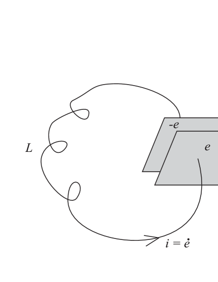
Figure 1: A single $LC$-circuit with an inductance $L$ and a capacitance $C$. The Lagrangian (20) gives the dynamics for $n$ interacting circuits of this type.

$$C^{-1}_{kl}=C^{-1}_{lk}\equiv\Gamma_{k\,l}+\Gamma_{k+n\,l+n}-\Gamma_{k\,l+n}-\Gamma_{l\,k+n},$$ (19)

where $k,l=1,\ldots,n$. Using this our Lagrangian (18) can be written,

$${\cal L}_{\rm LC}(e,\dot{e})=\frac{1}{2}\sum_{k=1}^{n}\sum_{l=1}^{n}\left(L_{kl}\dot{e}_{k}\dot{e}_{l}-C^{-1}_{kl}e_{k}e_{l}\right).$$ (20)

Here the $n$ charges $e_{k}$ and currents $\dot{e}_{k}$ are independent and a diagonal element of the $L$ matrix, $L_{kk}$, is a self-inductance, while the off diagonal elements correspond to mutual inductances. A diagonal element, $C^{-1}_{kk}=\Gamma_{k\,k}+\Gamma_{k+n\,k+n}-2\Gamma_{k\,k+n}$, of the $C^{-1}$-matrix represents the inverse capacitance, $C_{kk}$, of the corresponding conductor pair condenser.

3.2 Equivalence of electric and mechanical oscillators

The Lagrangian (20) is completely equivalent to that of a mechanical system of coupled oscillators, the $L$-matrix corresponding to the mass matrix and the $C^{-1}$-matrix corresponding to the stiffness matrix (of spring constants). This is often regarded as a purely formal correspondence, a mere mathematical mapping of one problem on another physically completely different one. This is wrong, however. If we denote the linear density of conducting charge in wire $k$ by $\lambda_{k}$, and the arc length along this wire by $s_{k}$, we find that the current in the wire is, $i_{k}=\dot{e}_{k}=\lambda_{k}\dot{s}_{k}$. Here, of course, $\dot{s}_{k}$ is the speed of the conducting linear charge density. Clearly the charges on the condensers have to be, $e_{k}=\lambda_{k}s_{k}$ (with a suitable choice of origin and orientation for the arc length). If this is inserted in ${\cal L}_{\rm LC}$ we find that,

$${\cal L}_{\rm LC}(e,\dot{e})=\frac{1}{2}\sum_{k=1}^{n}\sum_{l=1}^{n}\lambda_{k}\lambda_{l}\left(L_{kl}\dot{s}_{k}\dot{s}_{l}-C^{-1}_{kl}s_{k}s_{l}\right)\equiv$$

(21)

$$\frac{1}{2}\sum_{k=1}^{n}\sum_{l=1}^{n}\left(M_{kl}\dot{s}_{k}\dot{s}_{l}-K_{kl}s_{k}s_{l}\right)=T(\dot{s})-V(s)={\cal L}(s,\dot{s}).$$

The generalized coordinates $s_{k}$ now have dimension length so we have an ordinary mechanical coupled oscillator Lagrangian on the right hand side. The difference is that the mass matrix, $M_{kl}=\lambda_{k}\lambda_{l}L_{kl}$, does not come from rest mass but entirely from the inertia contained in the energy of the magnetic field.

By means of the technique of simultaneous diagonalization of two quadratic forms one can find a linear transformation to, so called, normal mode coordinates and thus decouple the equations of motion, which are,

$$\sum_{l=1}^{n}\left(L_{kl}\ddot{e}_{l}+C^{-1}_{kl}e_{l}\right)=0,\;\;\;k=1,\ldots,n,$$ (22)

assuming that no further generalized forces enter the problem. In terms of the normal modes $q_{k}$ the equations of motion become,

$$\ddot{q}_{k}+\frac{1}{L_{k}C_{k}}q_{k}=0,\;\;\;k=1,\ldots,n,$$ (23)

so these oscillate independently with angular frequencies $\omega_{k}=1/\sqrt{L_{k}C_{k}}$. For the corresponding mechanical problem one finds $\omega_{k}=\sqrt{K_{k}/M_{k}}$. The expression $\omega=1/\sqrt{LC}$ for the angular frequency of a single $LC$-circuit, as shown in Fig. 1, is sometimes referred to as Thomson’s formula.

3.3 Introduction of resistance and external voltage

Our Lagrangian (20) corresponds to a coupled system of undamped electromagnetic oscillators. In most cases of practical interest the connecting wires will not be perfectly conducting. There will be resistance in the system. The energy will then dissipate and the equations of motion require that there are generalized forces that describe this. Assume that the ohmic resistance in wire $k$ is $R_{kk}$. This can be achieved with a Rayleigh dissipation function. In a more general case there may also be off diagonal elements $R_{kl}$, and,

$${\cal R}(\dot{e})=\frac{1}{2}\sum_{k=1}^{n}\sum_{k=l}^{n}R_{kl}\dot{e}_{k}\dot{e}_{l},$$ (24)

is the most general form of this function for linear circuits.

If there is resistance currents $\dot{e}_{k}$ eventually dissipate to zero and arbitrary initial conditions only lead to transient dynamics. In most applications of circuit theory one is therefore mainly interested in systems with added external e.m.f.. This can be done by the additional term,

$${\cal L}_{\rm emf}(t)=\sum_{k=1}^{n}e_{k}\,{\cal V}_{k}(t),$$ (25)

added to the Lagrangian ${\cal L}_{\rm LC}$. Here ${\cal V}_{k}(t)$ is an applied external voltage. A constant e.m.f. will not drive a stationary current through a condenser so to get a direct current some of the $C^{-1}$-matrix eigenvalues must be zero. With harmonically oscillating e.m.f., ${\cal V}_{k}(t)={\cal V}_{k}\sin(\omega t)$, capacitors are no problem and one is dealing with alternating current circuits.

The general Lagrangian equations of motion for a system of circuits are then,

$$\frac{{\rm d}}{{\rm d}t}\frac{\partial{\cal L}_{\rm cc}}{\partial\dot{e}_{k}}-\frac{\partial{\cal L}_{\rm cc}}{\partial e_{k}}=-\frac{\partial{\cal R}}{\partial\dot{e}_{k}},$$ (26)

where,

$${\cal L}_{\rm cc}(e,\dot{e},t)={\cal L}_{\rm LC}(e,\dot{e})+{\cal L}_{\rm emf}(e,t),$$ (27)

is the circuit Lagrangian [24]. The system (22) of equations of motion are then modified so that,

$$\sum_{l=1}^{n}\left(L_{kl}\ddot{e}_{l}+R_{kl}\dot{e}_{l}+C^{-1}_{kl}e_{l}\right)={\cal V}_{k}(t),\;\;\;k=1,\ldots,n,$$ (28)

is their new form. This is thus the type of system investigated in linear circuit theory (see e.g. Guillemin [23] or Josephs [26]). In mechanical systems the ohmic resistance terms correspond to dampers (dashpots) and the external e.m.f. to applied external force.

3.4 Energy and Hamiltonian for conservative systems

For Lagrangians ${\cal L}(q,\dot{q})$ with no explicit time dependence, such as those of Eqs. (11) and (20), the quantity,

$${\cal E}(q,\dot{q})=\sum_{k=1}^{n}\frac{\partial{\cal L}}{\partial\dot{q}_{k}}\dot{q}_{k}-{\cal L},$$ (29)

is known to be a constant of the motion, the energy. For example the Darwin Lagrangian (11) corresponds to the conserved energy,

$${\cal E}_{D}={\cal E}_{\rm m}+\frac{1}{2}\sum_{a=1}^{N}\left(\frac{1}{c}e_{a}\mbox{\boldmath$v$}_{a}\cdot\mbox{\boldmath$A$}_{a}(\mbox{\boldmath$r$}_{a})+e_{a}\phi_{a}(\mbox{\boldmath$r$}_{a})\right).$$ (30)

This expression for the energy goes up if currents are parallel since the vector potential is proportional to terms like $e_{b}\mbox{\boldmath$v$}_{b}$. This may seem odd since we find in Sec. 4.3 that parallel currents attract. We will return to this in Sec. 5 below.

Returning to circuits we find that, when there is no time dependent forcing and no ohmic resistance, the Lagrangian is such that there is a conserved energy. Using (20) and (29) gives the expression,

$${\cal E}_{\rm LC}(e,\dot{e})=\frac{1}{2}\sum_{k=1}^{n}\sum_{l=1}^{n}\left(L_{kl}\dot{e}_{k}\dot{e}_{l}+C^{-1}_{kl}e_{k}e_{l}\right),$$ (31)

for this energy. Recall that if ${\cal L}=T-V$, then ${\cal E}=T+V$. The effect of a constant forcing, due to permanent constant charge on condensers, is only to shift the equilibrium from $e_{k}=\dot{e}_{k}=0$. Ignoring this (20) is the most general circuit Lagrangian that conserves the energy (31).

The generalized momenta obtained from the Lagrangian (20) are by definition,

$$p_{k}\equiv\frac{\partial{\cal L}_{\rm LC}}{\partial\dot{e}_{k}}=\sum_{l=1}^{n}L_{kl}\dot{e}_{l}.$$ (32)

The Hamiltonian is obtained by eliminating the generalized velocities in the Lagrangian energy (31) in favor of the generalized momenta. Since, $\dot{e}_{k}=\sum_{l=1}^{n}L^{-1}_{kl}p_{l}$, the Hamiltonian will depend on the inverse of the $L$-matrix. For a system of coupled $LC$-circuits we find the Hamiltonian,

$${\cal H}_{\rm LC}(e,p)=\frac{1}{2}\sum_{k=1}^{n}\sum_{l=1}^{n}\left(L^{-1}_{kl}p_{k}p_{l}+C^{-1}_{kl}e_{k}e_{l}\right),$$ (33)

representing its conserved energy as a function of phase space variables. The Lagrangian and Hamiltonian above, as well as the interpretation of the canonical momenta as magnetic fluxes discussed below, can be found in an article by Meixner [27], discussing thermodynamic issues.

3.5 Generalized momenta and magnetic flux

To find the meaning of the generalized, or canonical, momenta in this case we return to the definition of the magnetic Lagrangian,

$${\cal L}_{\rm L}=\frac{1}{2}\int\frac{1}{c}\mbox{\boldmath$j$}\cdot\mbox{\boldmath$A$}\,{\rm d}V.$$ (34)

The volume integration is only over the filamentary wires that carry the currents $i_{k}=\dot{e}_{k}$, so, using $\mbox{\boldmath$j$}\,{\rm d}V=i_{k}{\rm d}\mbox{\boldmath$r$}$, we get,

$${\cal L}_{\rm L}=\frac{1}{2c}\sum_{k=1}^{n}i_{k}\oint_{k}\mbox{\boldmath$A$}\cdot{\rm d}\mbox{\boldmath$r$},$$ (35)

where the line integral is around the loop of wire $k$. Now, however,

$$\oint_{k}\mbox{\boldmath$A$}\cdot{\rm d}\mbox{\boldmath$r$}=\int_{k}(\nabla\times\mbox{\boldmath$A$})\cdot{\rm d}\mbox{\boldmath$s$}=\int_{k}\mbox{\boldmath$B$}\cdot{\rm d}\mbox{\boldmath$s$},$$ (36)

according to Stokes’ theorem. By definition this is the magnetic flux, $\Phi_{k}$, through the loop $k$. We thus find that,

$${\cal L}_{\rm L}=\frac{1}{2}\sum_{k=1}^{n}i_{k}\frac{\Phi_{k}}{c}.$$ (37)

Comparing with (16) this gives us that,

$$\frac{\Phi_{k}}{c}=\sum_{l=1}^{n}L_{kl}i_{l}=p_{k},$$ (38)

where the individual terms on in the sum represent contributions to the flux through $k$ from the loops $l$ of the system.

Finally then, we have found that the generalized (canonical) momenta $p_{k}$, of Eq. (32), conjugate to the charges $e_{k}$ on the condensers are the magnetic fluxes through the currents loops (divided by $c$): $p_{k}=\Phi_{k}/c$. This means that if one $e_{l}$ does not appear in the Lagrangian (because there is no condenser in the corresponding loop) then that generalized momentum $p_{l}$ (or flux) is a constant of the motion.

4 Electromechanical systems

Few texts derive of equations of motion for electromechanical systems from the fundamental Lagrangian for particles and fields, only Neĭmark and Fufaev [28] come close. As should be clear from the above developments electromechanical systems, as opposed to electric circuits, require that we retreat from (15) back to the Darwin Lagrangian in the form (7), which we had before we neglected rest mass inertia. From there the equations of motion for electromechanical systems can be found by adding constraints, or assumptions, about the motion, thereby reducing the number of degrees-of-freedom, in the way familiar from analytical mechanics.

If macroscopic matter moves one must, of course, add the Lagrangian corresponding to that motion. Further, the induction and capacitance coefficients may now depend on the mechanical degrees-of-freedom corresponding to the motion of thin wires and extended conductors of the system, since this changes its geometry. For an energy conserving system one then typically arrives at a Lagrangian of the form,

$${\cal L}(q,e,\dot{q},\dot{e})=T(q,\dot{q})-V(q)+\frac{1}{2}\sum_{k=1}^{n}\sum_{l=1}^{n}\left[L_{kl}(q)\dot{e}_{k}\dot{e}_{l}-C^{-1}_{kl}(q)e_{k}e_{l}\right],$$ (39)

and this will be general enough for our purposes. One notes that if charged conductors move this produces magnetic effects which may have to be handled. In many cases, however, the speed of this motion will be such that the magnetic effect is negligible. In more general cases one may, of course, also have coupling terms between $\dot{q}$ and $\dot{e}$. In case of doubt the safe method is to start with the Darwin Lagrangian (11) and introduce relevant constraints and idealizations. A couple of examples of this procedure can be found in Essén [29, 30].

Electromechanical systems are treated e.g. in the books by Neĭmark and Fufaev [28], Wells [31], and Gossick [32]. Articles discussing various aspects of these systems are [33, 34, 35, 36]. We now proceed to some concrete examples of magnetomechanical systems.

4.1 Extension of current carrying ring

When a current $i$ flows in a conducting circular loop, or ring, its radius will increase somewhat. This is due to the reaction forces to the forces needed to bend the current that, due to inductive inertia, otherwise would move in a straight line. Let us calculate this increase in radius.

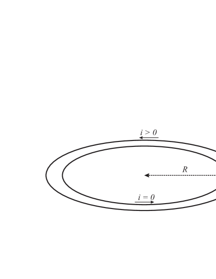
Figure 2: Notation for the ring extension problem. When the current $i=\dot{e}$ flowing in the ring is zero its radius is $R$. When the current is increased the radius becomes $R+\delta R=R(1+\xi)$.

The self-inductance of a ring made of thin wire of circular cross-section is, see Appendix A.3 below,

$$L_{\rm c}(R)=4\pi R\,[\,\ln(8R/\lambda)-(7/4)]/c^{2},$$ (40)

where $R$ is the ring radius (at zero current), and $\lambda$ is the radius of the thin wire. Assume that the wire ring can be treated as an elastic with stiffness $k$. The energy required to increase its length, $\ell=2\pi R$, by $\delta\ell=2\pi\,\delta R$ is then,

$$V(\delta R)=\frac{1}{2}k(\delta\ell)^{2}=\frac{1}{2}k(2\pi)^{2}(\delta R)^{2}.$$ (41)

If we introduce the notation, $\kappa=4\ln(8R/\lambda)$, and, $\xi=\delta R/R$, for the relative change in radius, we get the self-inductance,

$$L_{\rm c}(\xi)=\pi R(1+\xi)\,[(\kappa-7)+4\ln(1+\xi)]/c^{2},$$ (42)

for a ring as a function of the relative extension $\xi$ of the radius. The elastic potential energy is,

$$V(\xi)=\frac{1}{2}k(\delta\ell)^{2}=\frac{1}{2}k\,\ell^{2}\xi^{2},$$ (43)

where $k$ is the stiffness, or spring constant. We can now study the this two degree-of-freedom magnetomechanical system, the degrees-of-freedom being $e$, with $i=\dot{e}$, and $\xi$.

The Lagrangian will have the form given in Eq. (39) and becomes,

$${\cal L}(\xi,\dot{\xi},\dot{e})=\frac{1}{2}mR^{2}\dot{\xi}^{2}-V(\xi)+\frac{1}{2}L_{\rm c}(\xi)\dot{e}^{2},$$ (44)

where the first term is the kinetic energy of the ring, of mass $m$, due to time dependent radius. The corresponding Hamiltonian, including the kinetic energy of radial ring oscillations, the elastic energy, and the magnetic energy, is thus,

$${\cal H}(\xi,p_{\xi},p)=\frac{p_{\xi}^{2}}{2mR^{2}}+\frac{1}{2}k\,\ell^{2}\xi^{2}+\frac{p^{2}}{2L_{\rm c}(\xi)}.$$ (45)

Here $p=L_{\rm c}\dot{e}$ is the magnetic flux, divided by $c$, through the ring due to the current $\dot{e}=i$. The generalized momentum, $p_{\xi}=mR^{2}\dot{\xi}$, is the momentum of corresponding to radial motion of the ring.

Assume that we increase the flux, $p$, through the ring slowly without exciting radial oscillations. We might think of it as lying on a horizontal lubricated surface that dissipates kinetic energy keeping $p_{\xi}=0$. Let us calculate the ring extension. It will correspond to the minimum of the sum of the elastic and the magnetic energies ($\ell=2\pi R$),

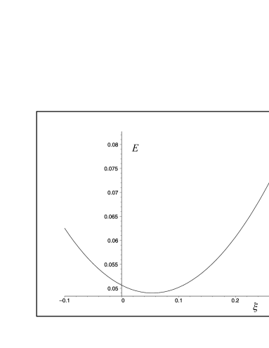
Figure 3: The function $E(\xi,p)$ of equation (46) plotted for $R=100\lambda$, so that $\kappa\approx 27$, and with, $k=\ell=p=c=1$, as a function of $\xi$.

$$E(\xi,p)=\frac{k}{2}(\ell\xi)^{2}+\frac{p^{2}c^{2}}{\ell(1+\xi)\,[(\kappa-7)+4\ln(1+\xi)]},$$ (46)

since this minimum corresponds to the minimum of the effective potential for the $\xi$-motion, $p$ being a constant of the motion. A graph of this function is shown in Fig. 3.

We first differentiate $E(\xi,p)$ with respect to $\xi$. To find the minimum we then wish to solve, ${\rm d}E/{\rm d}\xi=0$, for $\xi$, but this equation does not give any simple analytic root. We therefore first expand in the presumably small parameter $\xi$ and keep the constant and the linear term. The resulting equation is trivial to solve. Some algebraic rewriting make it possible to write the root in the form,

$$\xi_{0}(p)=\frac{(\kappa-3)(\kappa-7)c^{2}p^{2}}{(\kappa-7)^{3}\ell^{3}k+2[7+(\kappa-4)^{2}]c^{2}p^{2}},$$ (47)

where $\kappa=4\ln(8R/\lambda)$. This is thus, to first order, the relative extension, $\xi=\delta R/R$, of a conducting ring of radius $R$, cross-sectional radius $\lambda$, and elastic constant (stiffness) $k$, through which the current, $i=p/L_{\rm c}$, flows. The ring extension problem is also treated in Landau and Lifshitz, vol. 8 [24], but in a more complicated way.

4.2 Parallel coaxial circular current loops

The mutual inductance of two parallel coaxial rings, of radius $R_{1}$ and $R_{2}$, a distance $z$ apart, is given by (Becker [37]),

$$L_{12}=\frac{2\pi}{c^{2}}\int_{0}^{2\pi}\frac{R_{1}R_{2}\cos\varphi\,{\rm d}\varphi}{\sqrt{z^{2}+R_{1}^{2}+R_{2}^{2}-2R_{1}R_{2}\cos\varphi}}.$$ (48)

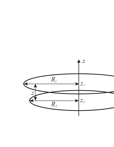
Figure 4: Notation for the two ring interaction problem. It is assumed that they can slide freely along the $z$-axis remaining parallel and coaxial. They have radii $R_{1}$ and $R_{2}$ and the distance between their planes is $z=z_{1}-z_{2}$. The currents in them are $i_{k}=\dot{e}_{k},\;k=1,2.$

The integral can be evaluated exactly in terms the complete elliptic integrals,

$${\rm K}(k) = \int_{0}^{\pi/2}\frac{{\rm d}\theta}{\sqrt{1-k^{2}\sin^{2}\!\theta}},$$ (49)

$${\rm E}(k) = \int_{0}^{\pi/2}\sqrt{1-k^{2}\sin^{2}\!\theta}\,{\rm d}\theta.$$ (50)

Putting,

$$k=\sqrt{\frac{4R_{1}R_{2}}{(R_{1}+R_{2})^{2}+z^{2}}}$$ (51)

one obtains,

$$L_{12}=\frac{4\pi}{c^{2}}\sqrt{R_{1}R_{2}}\left\{\frac{2}{k}\left[{\rm K}(k)-{\rm E}(k)\right]-k{\rm K}(k)\right\},$$ (52)

for the mutual inductance.

Assuming that the rings can slide along the $z$-axis we now get the Lagrangian ${\cal L}={\cal L}(z_{1},z_{2},\dot{z}_{1},\dot{z}_{2},\dot{e}_{1},\dot{e}_{2})$ of this four degree-of-freedom system in the form,

$${\cal L}=\frac{1}{2}m_{1}\dot{z}_{1}^{2}+\frac{1}{2}m_{2}\dot{z}_{2}^{2}+\frac{1}{2}L_{\rm c1}\dot{e}_{1}^{2}+\frac{1}{2}L_{\rm c2}\dot{e}_{2}^{2}+L_{12}(z_{1}-z_{2})\dot{e}_{1}\dot{e}_{2}.$$ (53)

We first do the well known transformation to center of mass and relative coordinates: $Z=(m_{1}z_{1}+m_{2}z_{2})/M,z=z_{1}-z_{2}$, where $M=m_{1}+m_{2}$. The Lagrangian ${\cal L}={\cal L}(z,\dot{z},\dot{Z},\dot{e}_{1},\dot{e}_{2})$ is now,

$${\cal L}=\frac{1}{2}M\dot{Z}^{2}+\frac{1}{2}m\dot{z}^{2}+\frac{1}{2}L_{\rm c1}\dot{e}_{1}^{2}+\frac{1}{2}L_{\rm c2}\dot{e}_{2}^{2}+L_{12}(z)\dot{e}_{1}\dot{e}_{2},$$ (54)

where $m=m_{1}m_{2}/M$ is the reduced mass. We now study this system.

4.3 Force per length between parallel constant currents

First, assume that, we maintain constant current in both rings: $\dot{e}_{k}=I_{k},\;k=1,2$. We note that this is a holonomic (integrable) constraint since it can be integrated to give, $e_{k}=e_{k}(0)+I_{k}t$, for the generalized coordinates. It is thus holonomic, but not time-independent (i.e. not scleronomic in traditional terminology). Since we will mostly introduce this constraint here for cyclic (ignorable) coordinates, i.e. coordinates that do not appear explicitly in the Lagrangian, the time dependence of the constraint will not be manifest in the appearance of Lagrangian. This is a peculiarity of the type of system treated here, which thus may formally appear conservative, even though it is not physically conservative. External energy is normally needed to maintain constant current, even for ideal conductors.

With this constraint there are only two degrees-of-freedom, $Z$ and $z$, and the Lagrangian (54) gives,

$${\cal L}=\frac{1}{2}M\dot{Z}^{2}+\frac{1}{2}m\dot{z}^{2}+I_{1}I_{2}L_{12}(z),$$ (55)

where we have discarded the two constants due to the self inductances. This is now a simple system in which the center of mass $Z$-motion is trivial, and where $V_{I}(z)=-I_{1}I_{2}L_{12}(z)$ acts as potential energy of the $z$-motion. Assuming that $R_{1}=R_{2}=R$ and that $z\ll R$ we find from expansion that,

$$L_{12}(z)\approx\frac{4\pi R}{c^{2}}\left[\ln\left(\frac{8R}{z}\right)-2\right]=-\frac{4\pi R}{c^{2}}\ln z+\,\mbox{constant}.$$ (56)

We throw away the constant term and find, in this approximation, the potential for the relative motion,

$$V_{I}(z)=\frac{4\pi R}{c^{2}}I_{1}I_{2}\ln z.$$ (57)

This means that,

$$\frac{F}{\ell}=-\frac{1}{2\pi R}\frac{{\rm d}V_{I}}{{\rm d}z}=-\frac{2}{c^{2}}\frac{I_{1}I_{2}}{z}$$ (58)

is the force per unit length between the rings (of length $\ell=2\pi R$) assuming $z\ll R$. One recognizes this as the standard expression for the force per length between parallel currents. The minus sign means that it is attractive when $I_{1}I_{2}>0$, i.e. for parallel currents, otherwise repulsive. This force between parallel current carrying wires has been much discussed in the pedagogical literature [38, 39, 40, 41, 42, 43] but the analytical mechanical approach presented here does not seem to have received much attention. The importance of the problem originates in the fact that the definition of the ampere, the SI unit of electric current, is based on this type of force measurement.

4.4 Relative oscillation of two rings of current

Assuming constant currents is not natural in this type of problems where we assume energy conservation. In general maintaining constant current requires that work is done by an external e.m.f.. For two perfectly conducting rings of modest size it is more natural to assume an isolated system of constant energy. We return to the Lagrangian (54) and note that since the coordinates (charges) $e_{1}$ and $e_{2}$ do not appear, the corresponding generalized momenta, $p_{1}$ and $p_{2}$, given by,

$$\frac{\partial{\cal L}}{\partial\dot{e}_{1}}\equiv p_{1}=L_{\rm c1}\,\dot{e}_{1}+L_{12}(z)\,\dot{e}_{2},\;\;\;\frac{\partial{\cal L}}{\partial\dot{e}_{2}}\equiv p_{2}=L_{\rm c2}\,\dot{e}_{2}+L_{12}(z)\,\dot{e}_{1},$$ (59)

are conserved. Solving these for the currents,

$$\dot{e}_{1}=\frac{L_{\rm c2}\,p_{1}-L_{12}(z)\,p_{2}}{L_{\rm c1}L_{\rm c2}-L^{2}_{12}(z)},\;\;\;\dot{e}_{2}=\frac{L_{\rm c1}\,p_{2}-L_{12}(z)\,p_{1}}{L_{\rm c1}L_{\rm c2}-L^{2}_{12}(z)},$$ (60)

we can proceed to find the Hamiltonian corresponding to the Lagrangian (54). This gives,

$${\cal H}=\frac{p_{Z}^{2}}{2M}+\frac{p_{z}^{2}}{2m}+\frac{L_{\rm c2}p_{1}^{2}+L_{\rm c1}p_{2}^{2}-2L_{12}(z)p_{1}p_{2}}{2[L_{\rm c1}L_{\rm c2}-L^{2}_{12}(z)]}.$$ (61)

We now wish to compare the interaction of the two rings for the case of constant currents $\dot{e}_{1}=\dot{e}_{2}=I$, and for the case of constant momenta,

$$p_{1}=[L_{\rm c1}+L_{12}(0)]I,\;\;\;p_{2}=[L_{\rm c2}+L_{12}(0)]I,$$ (62)

assuming currents $I$ at $z=0$.

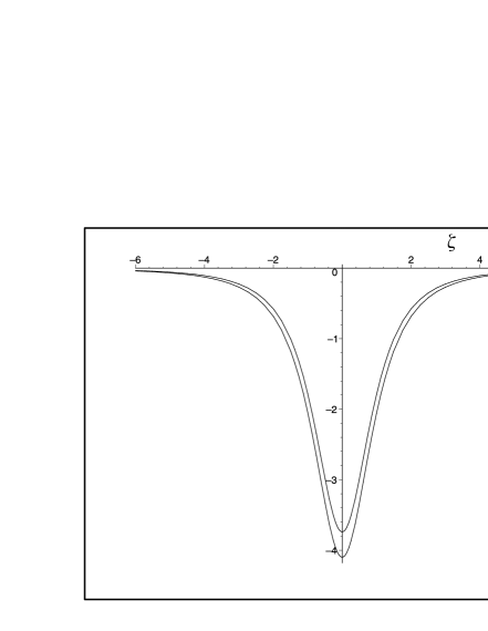
Figure 5: Plots of interaction potentials of two rings of current, see Fig. 4. For constant unit currents the potential is $V_{I}=-L_{12}(\zeta)$ and this is the upper curve. For constant generalized momenta, assuming unit currents at $z=\zeta=0$, the lower curve, corresponding to $V_{p}$ of Eq. (64), is obtained.

For constant currents the interaction potential is simply the negative of the last term of (54),

$$V_{I}(z)=-I^{2}L_{12}(z).$$ (63)

For the Hamiltonian (61) the potential that goes to zero at infinity is obtained by subtracting the constant, $\frac{p_{1}^{2}}{2L_{\rm c1}}+\frac{p_{2}^{2}}{2L_{\rm c2}}$, from the last term. This gives the potential,

$$V_{p}(z)=V_{I}(z)\frac{\left(1+\frac{L_{12}(0)}{L_{\rm c1}}\right)\left(1+\frac{L_{12}(0)}{L_{\rm c2}}\right)-\frac{L_{12}(z)}{2}\left[\frac{\left(1+\frac{L_{12}(0)}{L_{\rm c2}}\right)^{2}}{L_{\rm c1}}+\frac{\left(1+\frac{L_{12}(0)}{L_{\rm c1}}\right)^{2}}{L_{\rm c2}}\right]}{1-\frac{L^{2}_{12}(z)}{L_{\rm c1}L_{\rm c2}}},$$ (64)

for relative $z$-motion of the closed conservative system of two perfectly conducting rings.

To get definite results and compare the two expressions we now introduce specific values of the parameters. We use (40) for the self-inductances of the rings, $L_{\rm cj},\;j=1,2$, and expressions (51) and (52) for the mutual inductance $L_{12}(z)$ of the two rings. For definiteness we put, $R_{1}=\ell$, $R_{2}=(9/10)\ell$, $\lambda=\ell/20$, and use the dimensionless distance, $\zeta=z/\ell$, instead of the distance $z$ between the planes of the rings, see Fig. 4. With these choices, and putting $I=\ell=c=1$, we get the interaction potentials shown in Fig. 5. The difference is fairly small due two the fact that the self-inductances are an order of magnitude larger than the maximum value of the mutual inductance even though the parameters have been chosen to maximize the difference. A system for which the difference between a (time dependent) constant current constraint and a closed conservative system is, qualitatively and quantitatively, of importance is described in the following section.

4.5 Rectangular circuit and the rail gun

Here we study a system which can be thought of as an idealized rail gun. It reinforces the lesson in the ring extension example above in showing that closed loops of current tend to expand. In the example of the ring extension this can be understood as due to the inertia of the current. The current tries to go straight but has to follow the conducting wire and thus there must be a reaction force from the current on the wire that tends to straighten it out. Here we will see that this also happens when there are right angled corners in the circuit.

The self-inductance of a rectangular circuit with side lengths $a$ and $b$ made of flat conducting strips of width $\lambda$ in the plane of the rectangle has been calculated by Bueno and Assis [44, 45]. Their result is,

$$L_{\rm r}(a,b,\lambda)\approx\frac{1}{c^{2}}\left\{4\left[a\,\ln\left(\frac{2a}{\lambda}\right)+b\,\ln\left(\frac{2b}{\lambda}\right)\right]\right.$$

(65)

$$\left.-4\left[a\mbox{ arcsinh}\left(\frac{a}{b}\right)+b\mbox{ arcsinh}\left(\frac{b}{a}\right)\right]+8\sqrt{a^{2}+b^{2}}-2(a+b)\right\},$$

where the neglected terms are of order $\lambda\left\{{\cal O}[(\lambda/a)^{2}]+{\cal O}[(\lambda/b)^{2}]\right\}$. We now introduce $a=x=b\xi$ and $\lambda=b/10$ and assume that $\xi>1$ so that we can expand in $1/\xi$. This gives,

$$L_{\rm r}(\xi)\approx\frac{b}{c^{2}}\left([4\ln(10)+6]\,\xi+[4\ln(20)-2]-\frac{1}{\xi}+\frac{1}{24\xi^{3}}\right),$$ (66)

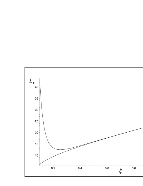
Figure 6: Comparison of the two approximations of the self-inductance $L_{\rm r}(\xi)$ of a rectangle. Here $b=c=1$ and the lower curve is the approximation in (65). The upper curve is the truncated series approximation in (66). The approximation is excellent for $0.5<\xi$.

where terms of order $1/\xi^{5}$ and higher have been neglected. The two expressions (65) and (66) are compared in the plot of Fig. 6.

The Lagrangian of the two degree-of-freedom system shown in Fig. 7 is then,

$${\cal L}=\frac{1}{2}mb^{2}\dot{\xi}^{2}+\frac{1}{2}L_{\rm r}(\xi)\dot{e}^{2},$$ (67)

where, $\dot{e}=i$, is the current in the circuit. The coordinate $e$ is absent (cyclic) so the generalized momentum,

$$p\equiv\frac{\partial{\cal L}}{\partial\dot{e}}=L_{\rm r}(\xi)\dot{e},$$ (68)

is conserved, assuming perfectly conducting parts. The conserved Hamiltonian becomes,

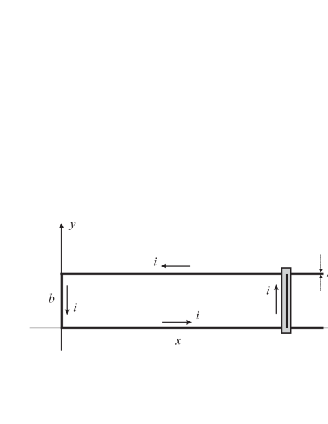
Figure 7: The self-inductance $L_{\rm r}$ of this rectangular current loop is given by Eq. (65) with $x=a$. A simple model of a rail gun is obtained when the right hand edge of the rectangle can slide, with negligible friction, in the direction of the $x$-axis.

$${\cal H}(\xi,p_{\xi},p)=\frac{1}{2}\frac{p_{\xi}^{2}}{mb^{2}}+\frac{1}{2}\frac{p^{2}}{L_{\rm r}(\xi)}=\frac{1}{2}\frac{p_{\xi}^{2}}{mb^{2}}+V_{p}(\xi),$$ (69)

where $p_{\xi}=mb^{2}\dot{\xi}$. Assume that $\dot{\xi}(0)=0$ at $\xi(0)=\xi_{0}$, so that the conserved energy, ${\cal H}=E$, is $E=\frac{p^{2}}{2{L_{\rm r}(\xi_{0})}}$. One then finds that,

$$v(\xi)=b\dot{\xi}(\xi)=p\sqrt{\frac{1}{m}\left(\frac{1}{L_{\rm r}(\xi_{0})}-\frac{1}{L_{\rm r}(\xi)}\right)},$$ (70)

is the velocity of the moving bar as function of $\xi=x/b$. Since the self-inductance goes to infinity with $\xi$ the limiting velocity of the bar will be $v(\infty)=p/\sqrt{mL_{\rm r}(\xi_{0})}$. The speed of the rail gun projectile is thus proportional to the conserved magnetic flux $\Phi=cp$ and inversely proportional to the square root of the self-inductance of the initial rectangle $L_{\rm r}(\xi_{0})$.

Assume instead that we maintain a constant current, i.e. introduce the constraint $\dot{e}=I$, in the rectangular circuit. A look at the Lagrangian (67) then shows that the there is, formally, a conserved energy,

$${\cal E}(\xi,\dot{\xi})=\frac{1}{2}mb^{2}\dot{\xi}^{2}-\frac{1}{2}I^{2}L_{\rm r}(\xi).$$ (71)

The bar will move in the potential $V_{I}(\xi)=-\frac{1}{2}I^{2}L_{\rm r}(\xi)$ and thus accelerate indefinitely (until the end of the rails). Though this still is formally a conservative system it is clear that energy must be continuously feed into the system to achieve the continuous acceleration of the bar. In fact charge in the system increases linearly, $e(t)=e(0)+It$, according to the implied time dependent constraint.

The treatment of the rail gun above is essentially new as far as the author knows, but this type of system has certainly been discussed both in the pedagogical and technical literature (see e.g. Knoepfel [46]). Some examples from pedagogical journals are [47, 48, 49]. Because of the many potential applications of rail guns there is a huge technical literature on the subject. A technical treatment using the Lagrangian formalism of electromechanical systems is by Hively and Condit [50].

5 On the nature of magnetic energy

It should be clear from the above examples that the methods of analytical mechanics can be quite useful in treating electromechanical, and in particular magnetomechanical, systems. There is no need to first find the fields and then the forces from these. Instead both steps are integrated into a single formalism.

While a Lagrangian with no explicit time dependence corresponds to a conservative system, one should note that a constant current constraint may only be formally energy conserving. External work may be needed to keep current constant. Consider the magnetic (inductive) part of the energy expression (31),

$${\cal E}_{\rm L}(q,\dot{e})=\frac{1}{2}\sum_{k=1}^{n}\sum_{l=1}^{n}L_{kl}(q)\dot{e}_{k}\dot{e}_{l},$$ (72)

where $q$ represents mechanical degrees-of-freedom. Should the currents be kept constant, $\dot{e}_{k}=I_{k}=$ constant, we find that this term becomes the negative of an effective potential for the $q$-motion,

$$V_{I}(q)=-\frac{1}{2}\sum_{k=1}^{n}\sum_{l=1}^{n}L_{kl}(q)I_{k}I_{l}=-{\cal E}_{\rm L}(q,I),$$ (73)

in a full Lagrangian of the form ${\cal L}_{I}(q,\dot{q})=T(\dot{q})-V_{I}(q)$. For this Lagrangian an equilibrium position corresponds to a minimum of $V_{I}(q)$. Evidently this corresponds to a maximum of the energy (72). We have thus arrived at the result that in electromechanical systems, for which current is kept constant, magnetic energy will tend to a maximum, when the system tends to its equilibrium.

The above result does not seem well known, even though explicitly stated in the textbook by Greiner [51]. It is also in accord with Woltjer’s [52] assumption that self organized states of a plasma should correspond to maxima of magnetic energy. Mehra and De Luca [53], on the other hand, made computer simulations of a plasma minimizing the velocity space form of the Darwin energy (30). They then found surprising results indicating that anti-parallel currents attracted each other. From our example above we know that it is the other way around. In conclusion, the velocity space form of the magnetic energy tends to become maximized.

Why would magnetic energy be so different from other forms of energy which usually tend to minima in equilibrium states? We can resolve this conundrum by recalling that there is also the Hamiltonian form of magnetic energy. The Hamiltonian corresponding to the Darwin energy is discussed in [54]. For circuits we have,

$${\cal H}_{\rm L}(q,p)=\frac{1}{2}\sum_{k=1}^{n}\sum_{l=1}^{n}L^{-1}_{kl}(q)p_{k}p_{l}.$$ (74)

We learned that the generalized momenta $p_{k}$, proportional to magnetic fluxes, are conserved if the corresponding charge $e_{k}$ is cyclic. For constant momenta $p_{k}=p^{0}_{k}$ the effective potential for the $q$-motion is,

$$V_{p}(q)={\cal H}_{\rm L}(q,p^{0}).$$ (75)

This form of the magnetic energy is minimized when the $q$-motion maximizes the inductive coefficients. The Hamiltonian and the Lagrangian formalisms thus correspond to two different energy concepts. In the case of magnetic energy, which is a kinetic energy, the coefficients of the generalized velocities, and the coefficients of the generalized momenta are each others inverse, which means that the minimum of one is the maximum of the other.

Schwinger et al. [6] is the only text that discusses the above facts concerning magnetic energy briefly. They also point out that the velocity space form of energy seems to give the erroneous idea that parallel currents repel. Being clear about which variables are held constant when one searches for a minimum is essential. Stating that magnetic energy is a maximum or a minimum for some configuration, as has been done [55], is meaningless unless this is made explicit.

Appendix A Appendices

Here the generalized capacitance coefficients and the inductance coefficients of linear circuit theory are derived and explained. Several results here are new. Even if the existence of these coefficients is stated in many texts, the discussion of their properties and physical origin usually is rather brief.

A.1 Energy of a system of charged conductors and generalized capacitance coefficients

Consider the electric energy expressed in the form,

$$W_{e}=\frac{1}{2}\int\varrho\phi\,{\rm d}V.$$ (76)

The potential, $\phi$, is a solution of Poisson’s equation,

$$\nabla^{2}\phi=-4\pi\varrho,$$ (77)

where it is assumed that the solution must go to zero at large distance from the region where the charge density, $\varrho$, is located. For point particles the solution to this equation is well known. Assuming that, $\varrho=\varrho_{i}(\mbox{\boldmath$r$})=e_{i}\delta(\mbox{\boldmath$r$}-\mbox{\boldmath$r$}_{i})$, the solution is, $\phi=\phi_{i}(\mbox{\boldmath$r$})=e_{i}/|\mbox{\boldmath$r$}-\mbox{\boldmath$r$}_{i}|$. For $N$ particles the charge density is the sum, $\varrho=\sum_{i}^{N}\varrho_{i}$, and the solution is simply a superposition of such solutions, $\phi(\mbox{\boldmath$r$})=\sum_{i}^{N}\phi_{i}$, due to the linearity of the Poisson’s equation. When these results are inserted into (76) one obtains the result,

$$W_{e}=\frac{1}{2}\sum_{i,j=1}^{N}\frac{e_{i}e_{j}}{r_{ij}},$$ (78)

where, $r_{ij}=|\mbox{\boldmath$r$}_{j}-\mbox{\boldmath$r$}_{i}|$, are the distances between the particles, and where it is necessary to exclude the case, $i=j$, to get a finite result.

Assume now that we, instead of particles, have a set of $n_{c}$ fixed conductors occupying the (compact) volumes $V_{k},\;(k=1,\ldots,n_{c})$ and ask: what is the potential $\phi$ and the energy $W_{e}$ of the system if we put charges $e_{k}$ on all, or some, of these (isolated) conductors? We know that the charge on each conductor must be distributed on its surface in such a way that the electric potential, $\phi(\mbox{\boldmath$r$})$, is constant on the surface, and the interior, of each conductor $V_{k}$. Otherwise current will flow until it becomes constant, since a gradient implies presence of electric field.

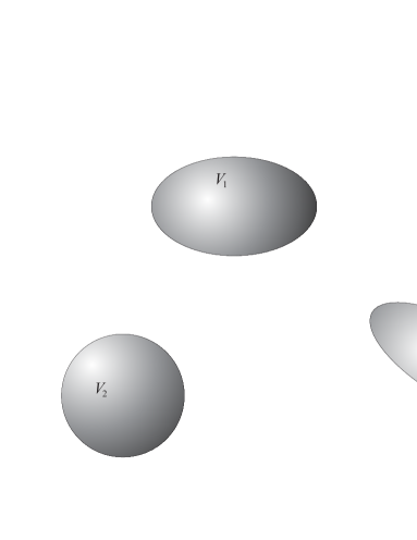
Figure 8: Here we study the potential arising from a system of conductors $V_{i}$ which either have a distribution $\varrho^{*}_{ii}$ of unit net charge or are only polarized with zero net charge redistributed to a density $\varrho^{*}_{ij}$, so as to make the potential constant on each conductor. In the figure $i,j=1,2,3$.

For the particle problem the charge density, $\varrho=\sum_{i}^{N}e_{i}\varrho^{*}_{i}$, with, $\varrho_{i}^{*}=\delta(\mbox{\boldmath$r$}-\mbox{\boldmath$r$}_{i})$, gave rise to the potential, $\phi=\sum_{i}^{N}e_{i}\phi_{i}^{*}$, where, $\phi^{*}_{i}=1/|\mbox{\boldmath$r$}-\mbox{\boldmath$r$}_{i}|$. We now wish to determine corresponding densities $\varrho_{i}^{*}$ and potentials $\phi_{i}^{*}$ for the case of isolated conductors, of given size, shape, and position. Assume that we place a unit charge on conductor $V_{i}$ while all the other conductors have zero charge. We first note that this does not mean that the charge densities on the other conductors are identically zero since charge on one of the conductors will induce a polarizing redistribution of the charge on the others. The total charge density for this case is thus,

$$\varrho^{*}_{i}=\sum_{k=1}^{n_{c}}\varrho^{*}_{ik},$$ (79)

where,

$$\int_{V}\varrho^{*}_{ik}{\rm d}V=\delta_{ik}=\left\{\begin{array}[]{ccc}1&\mbox{ if }&i=k\\ 0&\mbox{ if }&i\neq k\end{array}\right.$$ (80)

i.e. the net charge is unity on conductor $i$ and zero on the other conductors. Our assumption means that these densities must obey,

$$\nabla^{2}\phi^{*}_{i}=-4\pi\varrho^{*}_{i},$$ (81)

with $\phi^{*}_{i}(\mbox{\boldmath$r$})$ given by,

$$\phi^{*}_{i}(\mbox{\boldmath$r$})=\int_{V}\frac{\varrho_{i}^{*}(\mbox{\boldmath$r$}^{\prime})\,{\rm d}V^{\prime}}{|\mbox{\boldmath$r$}-\mbox{\boldmath$r$}^{\prime}|}=\sum_{k=1}^{n_{c}}\int_{V_{k}}\frac{\varrho^{*}_{ik}(\mbox{\boldmath$r$}_{k})\,{\rm d}V_{k}}{|\mbox{\boldmath$r$}-\mbox{\boldmath$r$}_{k}|}=\sum_{k=1}^{n_{c}}\phi^{*}_{ik}(\mbox{\boldmath$r$}),$$ (82)

and being such that,

$$\phi^{*}_{i}(\mbox{\boldmath$r$}_{j})=\Gamma_{ij}=\mbox{ const. for all }\;\mbox{\boldmath$r$}_{j}\in V_{j}.$$ (83)

Properly chosen $\varrho^{*}_{ij}$ must thus produce functions $\phi^{*}_{i}$ are constant on all of the conductors. One notes that the field $\phi^{*}_{ii}(\mbox{\boldmath$r$})$ has monopole character, while the $\phi^{*}_{ij}(\mbox{\boldmath$r$})$, for $i\neq j$, are of a dipole character.

The general solution to the Poisson equation (77) for a system of $n_{c}$ conductors with charges $e_{i}$ on the first $N(\leq n_{c})$ of them is then,

$$\phi(\mbox{\boldmath$r$})=\sum_{i=1}^{N}e_{i}\phi^{*}_{i}(\mbox{\boldmath$r$}),$$ (84)

according to the superposition principle. We see that the potentials $\phi^{*}_{i}$, arising from unit charge on conductor $i$ and zero on the rest, constitute a basis set of functions for this problem, analogous to the functions $\phi^{*}_{i}=1/|\mbox{\boldmath$r$}-\mbox{\boldmath$r$}_{i}|$ for the point particle problem.

Let us return, now to the energy expression Eq. (76). Since the charge density $\varrho$ is non-zero only on the conductors $V_{k}$ we find that

$$W_{e}=\frac{1}{2}\int\varrho\phi\,{\rm d}V=\frac{1}{2}\sum_{k=1}^{n_{c}}\int_{V_{k}}\varrho(\mbox{\boldmath$r$})\phi(\mbox{\boldmath$r$})\,{\rm d}V.$$ (85)

Use of (84) gives us,

$$W_{e}=\frac{1}{2}\sum_{k=1}^{n_{c}}\int_{V_{k}}\varrho(\mbox{\boldmath$r$})\sum_{i=1}^{N}e_{i}\phi^{*}_{i}(\mbox{\boldmath$r$})\,{\rm d}V,$$ (86)

but, since $\phi^{*}_{i}$ is constant on each of the conductors it can be taken out of the integral and replaced by its constant value on conductor $V_{k}$,

$$W_{e}=\frac{1}{2}\sum_{k=1}^{n_{c}}\sum_{i=1}^{N}e_{i}\phi^{*}_{i}(\mbox{\boldmath$r$}_{k})\int_{V_{k}}\varrho(\mbox{\boldmath$r$})\,{\rm d}V=\frac{1}{2}\sum_{j=1}^{N}\sum_{i=1}^{N}e_{i}\phi^{*}_{i}(\mbox{\boldmath$r$}_{j})e_{j}.$$ (87)

The second equality here is due to the fact that,

$$\varrho=\sum_{j=1}^{N}e_{j}\varrho_{j}^{*}=\sum_{j=1}^{N}e_{j}\sum_{l=1}^{n_{c}}\varrho^{*}_{jl},$$ (88)

so, according to (80), the integral of the charge density over $V_{k}$ is simply $e_{k}$, for $k=1,\ldots,N$, and zero for $k=N+1,\ldots,n_{c}$. So, using (83), we finally get,

$$W_{e}=\frac{1}{2}\sum_{i,j=1}^{N}\Gamma_{ij}e_{i}e_{j},$$ (89)

for the energy of the set of conducting bodies. When we compare this to (78) we see that the quantity $\Gamma_{ij}$ represents a kind of effective inverse distances between the charges on the conductors. As defined in (82 - 83) this quantity is the constant value of the potential on body $j$ when unit net charge is distributed on body $i$ and zero net charge on all the other $n_{c}-1$ bodies. Note that bodies with zero charge contribute to the values of the $\Gamma_{ij}$.

If we denote the constant value of the potential on conductor $i$ by $\phi_{i}=\phi(\mbox{\boldmath$r$}_{i})$ we find from (84) that,

$$\phi_{i}=\sum_{j=1}^{N}e_{j}\phi^{*}_{j}(\mbox{\boldmath$r$}_{i})=\sum_{j=1}^{N}e_{j}\Gamma_{ji},\;\;\;\mbox{ for }\;i=1,\ldots,N,$$ (90)

where (83) was used to get the last equality. These linear equations for the potentials can be solved for the charges. The result can be written,

$$e_{i}=\sum_{j=1}^{N}C_{ij}\phi_{j},\;\;\;\mbox{ for }\;i=1,\ldots,N,$$ (91)

where the coefficients $C_{ij}$ represent the matrix elements of the inverse of the matrix with elements $\Gamma_{ij}$. The $C_{ij}$ are called generalized capacitance coefficients.

A.2 Energy of a system of current carrying wires and the inductance coefficients

This is a subject discussed in many textbooks. Examples are Landau and Lifshitz, vol. 8 [24], Greiner’s Classical Electrodynamics [51], and Johnk [56]. A more specialized text is by Knoepfel [46].

The magnetic energy is given by,

$$W_{m}=\frac{1}{2c}\int\mbox{\boldmath$j$}\cdot\mbox{\boldmath$A$}\,{\rm d}V.$$ (92)

If one assumes that all current is flowing in thin wires one can replace the infinitesimal vector $\mbox{\boldmath$j$}\,{\rm d}V$ with $i_{k}\,{\rm d}\mbox{\boldmath$r$}_{k}$ where ${\rm d}\mbox{\boldmath$r$}_{k}$ is a line element along the curve $C_{k}$ defined by the $k$th wire (filament). This gives,

$$W_{m}=\frac{1}{2c}\sum_{k}i_{k}\int_{C_{k}}\mbox{\boldmath$A$}\cdot\,{\rm d}\mbox{\boldmath$r$}_{k}.$$ (93)

One notes immediately that if the curve is a closed curve the corresponding contribution is gauge independent since,

$$\oint_{C_{k}}\mbox{\boldmath$A$}\cdot\,{\rm d}\mbox{\boldmath$r$}_{k}=\oint_{C_{k}}(\mbox{\boldmath$A$}^{\prime}+\nabla\chi)\cdot\,{\rm d}\mbox{\boldmath$r$}_{k}=\oint_{C_{k}}\mbox{\boldmath$A$}^{\prime}\cdot\,{\rm d}\mbox{\boldmath$r$}_{k}.$$ (94)

For conducting wires that are not closed but instead go between conductors that provide capacitance the issue of gauge may need to be resolved.

When there is gauge independence we can use the expression,

$$\mbox{\boldmath$A$}(\mbox{\boldmath$r$})=\frac{1}{c}\int\frac{\mbox{\boldmath$j$}(\mbox{\boldmath$r$}^{\prime}){\rm d}V^{\prime}}{|\mbox{\boldmath$r$}-\mbox{\boldmath$r$}^{\prime}|}=\sum_{l}\frac{i_{l}}{c}\int_{C_{l}}\frac{{\rm d}\mbox{\boldmath$r$}_{l}}{|\mbox{\boldmath$r$}-\mbox{\boldmath$r$}_{l}|},$$ (95)

for the vector potential from the currents $i_{l}$ flowing in wires along the curves $C_{l}$. Inserting this into (96) we find that the magnetic energy is,

$$W_{m}=\frac{1}{2c^{2}}\sum_{kl}i_{k}i_{l}\int_{C_{k}}\int_{C_{l}}\frac{{\rm d}\mbox{\boldmath$r$}_{k}\cdot\,{\rm d}\mbox{\boldmath$r$}_{l}}{|\mbox{\boldmath$r$}_{k}-\mbox{\boldmath$r$}_{l}|}.$$ (96)

So, if we introduce the wire geometry dependent quantities,

$$L_{kl}=\frac{1}{c^{2}}\int_{C_{k}}\int_{C_{l}}\frac{{\rm d}\mbox{\boldmath$r$}_{k}\cdot\,{\rm d}\mbox{\boldmath$r$}_{l}}{|\mbox{\boldmath$r$}_{k}-\mbox{\boldmath$r$}_{l}|},$$ (97)

we find the magnetic energy in the form,

$$W_{m}=\frac{1}{2}\sum_{kl}L_{kl}i_{k}i_{l}.$$ (98)

For fixed positions of the wires the magnetic energy is thus a quadratic form in the currents with constant coefficients $L_{kl}$. For $l\neq k$ these are called mutual inductances. When $l=k$ they are self-inductances.

Apart from the problem of lack of gauge invariance for non-closed wires one must also deal somehow with the logarithmic divergence of the self-inductance for a truly filamentary wire. If the wire is assumed to be a mathematical curve of no thickness the expression (97) will diverge when $k=l$. Should one find a way to handle the divergence there remains the question of the gauge invariance of the self-inductances. Let us consider these questions by means of an example.

We first note that if the Darwin expression (9) for the vector potential, is used instead of (95), the induction coefficients become,

$$L_{kl}=\frac{1}{2c^{2}}\int_{C_{k}}\int_{C_{l}}\frac{{\rm d}\mbox{\boldmath$r$}_{k}\cdot\,{\rm d}\mbox{\boldmath$r$}_{l}+({\rm d}\mbox{\boldmath$r$}_{k}\cdot\mbox{\boldmath$e$}_{kl})({\rm d}\mbox{\boldmath$r$}_{l}\cdot\mbox{\boldmath$e$}_{kl})}{|\mbox{\boldmath$r$}_{k}-\mbox{\boldmath$r$}_{l}|},$$ (99)

i.e. different from the Neumann form (97).

A.3 Self-inductance of a rotating polygon of charged particles

One way of handling the divergence in the filamentary self-induction is to consider the current as due to many charged particles travelling in the wire, instead of a continuous distribution of charge. Assume that the current in a circular wire is due to $N$ particles of charge $e$ forming a regular polygon that rotates rigidly. We assume as usual that the material of the wire is of the opposite charge and cancels the charge of the particles so that effects of Coulomb interactions are negligible.

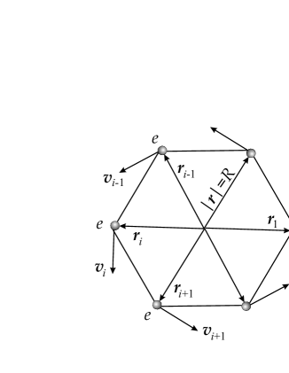
Figure 9: An example of a polygonal circular current with $N=6$.

Assuming that the circle has radius $R$, positions and velocities are given by,

$$\mbox{\boldmath$r$}_{i}(\varphi_{i})=R\mbox{\boldmath$e$}_{\rho}(\varphi_{i}),\hskip 8.5359pt\mbox{and}\hskip 8.5359pt\mbox{\boldmath$v$}_{i}(\varphi_{i},\dot{\varphi}_{i})=R\dot{\varphi}_{i}\mbox{\boldmath$e$}_{\varphi}(\varphi_{i}),$$ (100)

where, $\mbox{\boldmath$e$}_{\rho}(\varphi)=\cos\varphi\,\mbox{\boldmath$e$}_{x}+\sin\varphi\,\mbox{\boldmath$e$}_{y}$ and $\dot{\mbox{\boldmath$e$}}_{\rho}=\dot{\varphi}\mbox{\boldmath$e$}_{\varphi}$, as usual. If we further assume that all the angular velocities $\dot{\varphi}_{i}$ are the same, and given by $\dot{\varphi}_{i}=\omega$, and that the angles are $\varphi_{i}=(i-1)2\pi/N$ for $i=1,\ldots,N$, we have a rigidly rotating regular polygon. This is illustrated for $N=6$ in Fig. 9.

We now calculate the magnetic energy of this system and compare the expressions obtained using the two different expressions (9) and (95) for the vector potential. Simple calculations show that the magnetic energy can be written,

$$W_{m}=\frac{e}{2c}\sum_{i=1}^{N}v_{i}A_{i},$$ (101)

where all $v_{i}=R\dot{\varphi}_{i}=R\omega$, and where,

$$A_{i}=\frac{e}{cR}\sum_{j\neq i}^{N}v_{j}V_{\varphi}(\varphi_{i}-\varphi_{j}).$$ (102)

Here $V_{\varphi}$ is given by,

$$V_{\varphi}^{D}(\varphi)=\frac{1}{4}\frac{1+3\cos\varphi}{\sqrt{2(1-\cos\varphi)}},$$ (103)

in the Darwin case (13) and by,

$$V_{\varphi}^{L}(\varphi)=\frac{\cos\varphi}{\sqrt{2(1-\cos\varphi)}},$$ (104)

in the Lorenz case (95). Because of the symmetry all terms in the sum (101) are equal and we find,

$$W_{m}=\frac{1}{2}\frac{e^{2}}{R}\left(\frac{v}{c}\right)^{2}N^{2}\left(\frac{1}{2\pi}\sum_{i=1}^{N-1}V_{\varphi}(i\,\Delta\varphi)\Delta\varphi\right),$$ (105)

where $\Delta\varphi=2\pi/N$. We note that the current in the ring is $i=\frac{e\omega N}{2\pi}$ so we can write the above expression in the form $W_{m}=\frac{1}{2}Li^{2}$ where $L$, by definition, is the self-inductance,

$$L=\left(\frac{2\pi}{c}\right)^{2}R\,\frac{1}{2\pi}\sum_{i=1}^{N-1}V_{\varphi}(i\,\Delta\varphi)\Delta\varphi,$$ (106)

of the polygon.

For all but the smallest values of $N$ it is useful to approximate the sum with an integral. Using the trapezoidal rule [57],

$$\int_{a}^{b}f(x)\,{\rm d}x\approx\frac{b-a}{n}\left\{\frac{1}{2}f(a)+\sum_{k=1}^{n-1}f\left(a+k\frac{b-a}{n}\right)+\frac{1}{2}f(b)\right\},$$ (107)

we find that (taking $n=N-2$),

$$\sum_{i=1}^{N-1}V_{\varphi}(i\,\Delta\varphi)\Delta\varphi\approx\int_{\frac{2\pi}{N}}^{2\pi-\frac{2\pi}{N}}V_{\varphi}(\varphi)\,{\rm d}\varphi+\frac{\pi}{N}\left[V_{\varphi}\left(\frac{2\pi}{N}\right)+V_{\varphi}\left(2\pi-\frac{2\pi}{N}\right)\right].$$ (108)

Using this and expanding the result in powers of $1/N$ one finds the results,

$$L^{D}=\frac{4\pi}{c^{2}}R\left[\ln\left(\frac{2N}{\pi}\right)-1\right]$$ (109)

for the Darwin case (103), and,

$$L^{L}=\frac{4\pi}{c^{2}}R\left[\ln\left(\frac{2N}{\pi}\right)-\frac{3}{2}\right]$$ (110)

for the Lorenz case (104). The integral can be done analytically. Terms in $1/N^{4}$ and higher were neglected in the expansions. Maple [58] was used in these calculations, as well as for most other calculations and plots of this review.

These results may be compared with the traditional result (Becker [37]),

$$L_{\rm c}=\frac{4\pi}{c^{2}}R\left[\ln\left(\frac{8R}{\lambda}\right)-\frac{7}{4}\right],$$ (111)

for the self-inductance of a circular loop conductor used above in (40). Since $N=2\pi R/\delta$, where $\delta$ is the distance between neighboring charges along the circle, the logarithmic parts of the results agree if $\delta=\lambda/2$. Equivalently the polygon must have $N=4\pi R/\lambda$ electrons to agree with the logarithmic part of the ring result, $\lambda$ being the cross sectional radius of the ring.

For large $N$ the logarithmic part of the self-inductance should be the dominating one. The contributions linear in $R$ are seen to be different in all cases but do seem to have an order of magnitude agreement.

There is a considerable literature on inductance calculations. The books by Bueno and Assis [44] and by Grover [59] may be mentioned. Technical papers are [60, 61, 62], and a few applications of ideas concerning self-inductance can be found in [63, 64, 65].

References

- [1] James Clerk Maxwell. A Treatise on Electricity and Magnetism, Vols 1 and 2. Clarendon Press, Oxford, 3rd edition, 1891.
- [2] Charles Galton Darwin. The dynamical motions of charged particles. Phil. Mag. ser. 6., 39:537–551, 1920.
- [3] John David Jackson. Classical Electrodynamics. John Wiley & Sons, New York, 3rd edition, 1999.
- [4] L. D. Landau and E. M. Lifshitz. The Classical Theory of Fields. Pergamon, Oxford, 4th edition, 1975.
- [5] Emil Jan Konopinski. Electromagnetic Fields and Relativistic Particles. McGraw-Hill Book Company, Inc., New York, 1981.
- [6] Julian Schwinger, Lester L. DeRaad, Jr., Kimball A. Milton, and Wu-yang Tsai. Classical Electrodynamics. Perseus books, Reading, Massachusetts, 1998.
- [7] Wolfgang K. H. Panofsky and Melba Phillips. Classical Electricity and Magnetism. Dover, New York, 2nd edition, 2005.
- [8] Cornelius Lanczos. The Variational Principles of Mechanics. Dover, New York, 4th edition, 1986.
- [9] Wolfgang Yourgrau and Stanley Mandelstam. Variational Principles in Dynamics and Quantum Theory. Dover, New York, 3rd edition, 1968.
- [10] Noel A. Doughty. Lagrangian Interaction – An Introduction to Relativistic Symmetry in Electrodynamics and Gravitation. Westview Press, Reading, Massachusetts, 1990.
- [11] Boris Kosyakov. Introduction to the Classical Theory of Particles and Fields. Springer, Berlin, 2007.
- [12] Boris Podolsky and Kaiser S. Kunz. Fundamentals of Electrodynamics. Marcel Dekker, New York, 1969.
- [13] James L. Anderson and Samuel Schiminovich. Relations between field-plus source and Fokker-type action principles. J. Math. Phys., 8:255–264, 1967.
- [14] B. M. Barker and R. F. O’Connel. The post-post Newtonian problem in classical electromagnetic theory. Ann. Phys. (N.Y.), 129:358–377, 1980.
- [15] E. Breitenberger. Magnetic interactions between charged particles. Am. J. Phys., 36:505–515, 1968.
- [16] Hanno Essén. Darwin magnetic interaction energy and its macroscopic consequences. Phys. Rev. E, 53:5228–5239, 1996.
- [17] Hanno Essén. Magnetism of matter and phase-space energy of charged particle systems. J. Phys. A: Math. Gen., 32:2297–2314, 1999.
- [18] Frederick James Kennedy. Approximately relativistic interactions. Am. J. Phys., 40:63–74, 1972.
- [19] Todd B. Krause, A. Apte, and P. J. Morrison. A unified approach to the Darwin approximation. Phys. of Plasmas, 14:102112–1–10, 2007.
- [20] Jonas Larsson. Electromagnetics from a quasistatic perspective. Am. J. Phys., 75:230–239, 2007.
- [21] Charles Galton Darwin. The inertia of electrons in metals. Proc. R. Soc. Lond. A, 154:61–66, 1936.
- [22] Stig Lundquist. Magneto-hydrostatic fields. Ark. Fys., 2:361–365, 1950.
- [23] Ernst A. Guillemin. Introductory Circuit Theory. John Wiley & Sons, Inc., New York, 1953.
- [24] L. D. Landau and E. M. Lifshitz. Electrodynamics of Continuous Media. Butterworth-Heinemann, Oxford, 2nd edition, 1984.
- [25] Israel D. Vagner, Boris I. Lembrikov, and Peter Wyder. Electrodynamics of Magnetoactive Media. Springer, Berlin, 2004.
- [26] H. J. Josephs. Heaviside’s Electric Circuit Theory. Methuen, London, 1950.
- [27] J. Meixner. Thermodynamics of electrical networks and the Onsager-Casimir reciprocal relations. J. Math. Phys., 4:154–159, 1963.
- [28] Ju. I. Neimark and N. A. Fufaev. Dynamics of Nonholonomic Systems. Translations of Mathematical Monographs, vol. 33. American Mathematical Society, Providence, Rhode Island, 1972.
- [29] Hanno Essén. Electrodynamic model connecting superconductor response to magnetic field and to rotation. Eur. J. Phys., 26:279–285, 2005.
- [30] Hanno Essén. Magnetic dynamics of simple collective modes in a two-sphere plasma model. Phys. of Plasmas, 12:122101–1–7, 2005.
- [31] Dare A. Wells. Lagrangian Dynamics. McGraw-Hill, New York, 1967.
- [32] B. R. Gossick. Hamilton’s Principle and Physical Systems. Academic Press, New York, 1967.
- [33] D. A. Wells. Application of the Lagrangian equations to electrical circuits. J. Appl. Phys., 9:312–320, 1938.
- [34] G. W. Ogar and J. J. D’Azzo. A unified procedure for deriving the differential equations of electrical and mechanical systems. IRE Trans. Educ. (USA), pages 18–26, 1962.
- [35] V. Hadwich and F. Pfeiffer. The principle of virtual work in mechanical and electromechanical systems. Archive of Appl. Mech., 65:390–400, 1995.
- [36] D. Basic, F. Malrait, and P. Rouchon. Euler-Lagrange models with complex currents of three-phase electrical machines. E-print: arXiv:0806.0387v1 [math.OC], June 2008.
- [37] Richard Becker. Electromagnetic Fields and Interactions. Blaisdell, New York, 1964. Reprinted: Dover, New York, 1982.
- [38] David L. Webster. Relativity and parallel wires. Am. J. Phys., 29:841–844, 1961.
- [39] Allen Folmsbee and Thomas Moran. Demonstration of forces between parallel wires: Calibraition of an ammeter. Am. J. Phys., 45:106–107, 1977.
- [40] Denise C. Gabuzda. Magnetic force due to a current-carrying wire: A paradox and its resolution. Am. J. Phys., 55:420–422, 1987.
- [41] Denise C. Gabuzda. The charge densities in a current-carrying wire. Am. J. Phys., 61:360–362, 1993.
- [42] D. Amrani. Use of a current balance to calibrate an ammeter and to determine the magnetic permeability of free space. Eur. J. Phys., 26:273–278, 2005.
- [43] Paul van Kampen. Lorentz contraction and current-carrying wires. Eur. J. Phys., 29:879–883, 2008.
- [44] Marcelo de Almeida Bueno and Andre Koch Torres Assis. Inductance and Force Calculations in Electrical Circuits. Nova Science Publishers, Huntington, N.Y., 2001.
- [45] Marcelo A. Bueno and A. K. T. Assis. A new method for inductance calculations. J. Phys. D, 28:1802–1806, 1995.
- [46] Heinz E. Knoepfel. Magnetic Fields: A Comprehensive Theoretical Treatise for Practical Use. Wiley-Interscience, New York, 2000.
- [47] Victor Namias. Induced current effects in Faraday’s law and introduction to flux compression theories. Am. J. Phys., 54:57–69, 1986.
- [48] A. E. Robson and J. D. Sethian. Railgun recoil, ampere tension, and the laws of electrodynamics. Am. J. Phys., 60:1111–1117, 1992.
- [49] R. Jones. The rail gun: a popular demonstration of the Lorentz force. Am. J. Phys., 68:773–774, 2000.
- [50] Lee M. Hively and William C. Condit. Electromechanical railgun model. IEEE Trans. Magn., 27:3731–3734, 1991.
- [51] Walter Greiner. Classical Electrodynamics. Springer, New York, 1998.
- [52] L. Woltjer. A theorem on force-free magnetic fields. Proc. Nat. Acad. Sci., 44:489–491, 1958.
- [53] Vishal Mehra and Jayme De Luca. Long range magnetic order and the Darwin Lagrangian. Phys. Rev. E, 61:1199–1205, 2000.
- [54] Hanno Essén and Arne B. Nordmark. Hamiltonian of a homogeneous two-component plasma. Phys. Rev. E, 69:036404–1–9, 2004.
- [55] M. C. N. Fiolhais. Minimum magnetic energy theorem. E-print: arXiv:0811.2598v1 [physics.class-ph], November 2008.
- [56] Carl T. A. Johnk. Engineering Electromagnetic Fields and Waves. Wiley, New York, 1988.
- [57] Germund Dahlquist, Åke Björk, and Ned Anderson. Numerical Methods. Prentice-Hall, New Jersey, 1974.
- [58] André Heck. Introduction to Maple. Springer, Berlin, 3rd edition, 2003.
- [59] F. W. Grover. Inductance Calculations – Working Formulas and Tables. Van Nostrand, New York, 1946.
- [60] Milan Wayne Garrett. Calculation of fields, forces, and mutual inductances of current systems by elliptic integrals. J. Appl. Phys., 34:2567–2573, 1963.
- [61] F. B. J. Leferink. Inductance calculations; methods and equations. In Proceedings of International Symposium on Electromagnetic Compatibility, pages 16–22. IEEE, 1995.
- [62] A. Abakar, G. Meunier, J.-L. Coulomb, and F.-X. Zgainski. 3d modeling of thin wires interacting with thin plates: extracting the singularity due to the loop wire self inductance. Eur. Phys. J. Appl. Phys. (France), 14:63–67, 2001.
- [63] R. Rammal, T.C. Lubensky, and G. Toulouse. Superconducting networks in a magnetic field. Phys. Rev. B, Condens. Matter, 27:2820–9, 1983.
- [64] J.B. Pendry, A.J. Holden, W.J. Stewart, and I. Youngs. Extremely low frequency plasmons in metallic mesostructures. Phys. Rev. Lett., 76:4773–4776, 1996.
- [65] J. C. Flores and C. A. Utreras-Diaz. Mesoscopic circuits with charge discreteness: quantum current magnification for mutual inductances. Phys. Rev. B, Condens. Matter Mater. Phys., 66:1534–10–14, 2002.