End-to-End Outage Minimization in OFDM Based Linear Relay Networks

Abstract

Multi-hop relaying is an economically efficient architecture for coverage extension and throughput enhancement in future wireless networks. OFDM, on the other hand, is a spectrally efficient physical layer modulation technique for broadband transmission. As a natural consequence of combining OFDM with multi-hop relaying, the allocation of per-hop subcarrier power and per-hop transmission time is crucial in optimizing the network performance. This paper is concerned with the end-to-end information outage in an OFDM based linear relay network. Our goal is to find an optimal power and time adaptation policy to minimize the outage probability under a long-term total power constraint. We solve the problem in two steps. First, for any given channel realization, we derive the minimum short-term power required to meet a target transmission rate. We show that it can be obtained through two nested bisection loops. To reduce computational complexity and signalling overhead, we also propose a sub-optimal algorithm. In the second step, we determine a power threshold to control the transmission on-off so that the long-term total power constraint is satisfied. Numerical examples are provided to illustrate the performance of the proposed power and time adaptation schemes with respect to other resource adaptation schemes.

I Introduction

Relay networks in the form of point-to-multipoint based tree-type or multipoint-to-multipoint mesh-type architectures are a promising network topology in future wireless systems. The basic concept of relaying is to allow a source node to communicate with a destination node under the help of a single or multiple relay nodes. It has been shown that relaying can bring a wireless network various benefits including coverage extension, throughput and system capacity enhancement. Recently, multi-hop relaying has been widely adopted in wireless networks such as next generation cellular networks, broadband wireless metropolitan area networks and wireless local area networks. On the other hand, orthogonal frequency division multiplexing (OFDM) is an efficient physical layer modulation technique for broadband wireless transmission. It divides the broadband wireless channel into a set of orthogonal narrowband subcarriers and hence eliminates the inter-symbol interference. OFDM is one of the dominating transmission techniques in many wireless systems, e.g., IEEE 802.16 (WiMax), EV-DO Revision C and the Long-Term-Evolution (LTE) of UMTS. The combination of OFDM and multi-hop relaying has received a lot of attention recently. For example, this OFDM-based relay architecture has been proposed by the current wireless standard IEEE 802.16j [1]. The complexity of relay station is expected to be much less than the one of legacy IEEE 802.16 base stations, thereby reducing infrastructure deployment cost and improving the economic viability of IEEE 802.16 systems [2].

In this work, we are interested in an OFDM-based linear relay network. The so-called linear relay network consists of one-dimensional chain of nodes, including a source node, a destination node and several intermediate relay nodes. It can be viewed as an important special case of relay networks where only a single route is active. As a natural consequence of multi-hop relaying and OFDM transmission, the allocation of per-hop subcarrier power and per-hop transmission time is crucial in optimizing the end-to-end network performance.

Previous work on resource allocation for relay networks is found in [3, 4, 5, 6, 7, 8]. Yao et al. in [3] considered a classic three-node network (a source node, a destination node, and a relay node) and compared the energy required for transmitting one information bit in different relay protocols. Authors in [4] and [6] studied efficient scheduling and routing schemes in one-dimensional multi-hop wireless networks. It is assumed in all these works [4, 6, 3] that the point-to-point links are frequency-flat fading channels and the system has a fixed short-term power constraint. In [5], Oyman et al. summarized the end-to-end capacity results of a multi-hop relay network under fixed-rate and rate-adaptive relaying strategies, and further illustrated the merits of multi-hop relaying in cellular mesh networks. Authors in [9] studied the per-hop transmission time and subcarrier power allocation problem in the OFDM based linear multi-hop relay network to maximize the end-to-end average transmission rate under a long-term total power constraint. However, the end-to-end average rate can only be obtained at the expense of large delay.

For many real-time services, one has to maintain a target transmission rate and avoid service outage in most of fading condition through adaptive resource allocation. An outage is an event that the actual transmission rate is below a prescribed transmission rate ([10] and [11]). Outage probability can be viewed as the fraction of time that a codeword is decoded wrongly. For any finite average power constraint, transmission outage may be inevitable over fading channels. However, one can minimize the outage probability through adaptive power control [10]. In a relay network where no data is allowed to accumulate at any of relay nodes, an end-to-end outage is the event that there exists a hop over which the transmission rate is lower than the target rate.

The goal of this paper is to investigate the optimal per-hop power and time control to minimize the end-to-end outage probability in an OFDM linear relay network under an average transmission power constraint. At first, we derive the minimum short-term power required to meet a target transmission rate for any given channel realization. The resulting power and time allocation can be obtained through a Two-nested Binary Search (TBS) which is conducted in a central controller with the knowledge of channel state information (CSI) on all subcarriers and over all hops. Such algorithm gives a theoretical performance limit of linear relay networks, but is computationally intense. Moreover, it requires significant signalling overhead and channel feedback between network nodes and the central controller. For this reason, an Iterative Algorithm of Sub-optimal power and time allocation (IAS) is proposed. The required information for signalling exchange only involves the number of active subcarriers on each hop and the geometric mean and harmonic mean of channel gains averaged over the active subcarriers. This sub-optimal allocation algorithm suggests prolonging the transmission time for the hop with low geometric mean of channel gains while lowering the transmission power for the hop with low harmonic mean. After obtaining the minimum power required to support the target rate for a given channel realization, we then compare it with a threshold. The transmission will be cut off if the required minimum total power exceeds the threshold. The threshold takes the value so that the long-term total power constraint is satisfied. Numerical results show that a significant power saving can be achieved by the proposed optimal power and time allocation compared with the uniform power and time allocation under the same end-to-end outage probability. In addition, the proposed sub-optimal power and time allocation serves as a good approximation to the optimal solution when the target rate is sufficiently high. The optimal number of hops in the sense of requiring minimum power at different target rates is also shown numerically.

The remainder of this paper is organized as follows. In Section II, the system model and problem formulation are presented. The optimal and sub-optimal resource allocation algorithms to minimize the end-to-end outage probability under an average total power constraint are proposed in Section III. Numerical results are given in Section IV. Finally we conclude this paper in Section V.

II System model, end-to-end rate and outage probability

II-A System Model

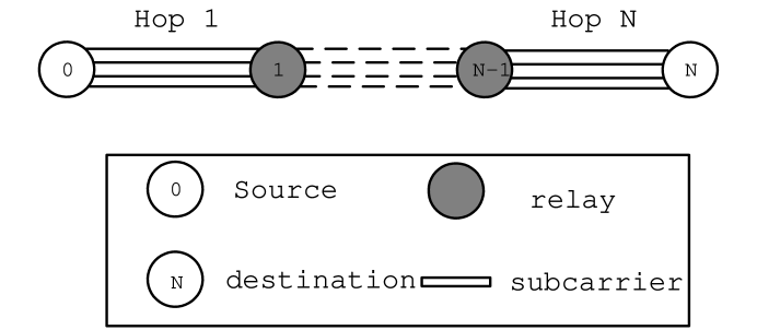
Figure 1: Illustration of linear relay networks

Consider a wireless linear relay network shown in Fig. 1. The source node $R_{0}$ communicates with destination $R_{N}$ by routing its data through $N-1$ intermediate relay nodes $R_{n}~{}(n=1,\ldots,N-1)$. The hop between node $R_{n-1}$ and $R_{n}$ is indexed by $n$, and the set of hops is denoted by $\mathcal{N}$. We focus on time-division based relaying. The transmission time is divided into frames of multiple time slots. Within every time frame, the transmission over each hop takes place at the assigned time slots. In general, frequency reuse can be applied so that more than one hop can be transmitting at a same time slot. However, due to interference issue, it will increase decoding complexity as well as decoding delay [4]. Thus, in this work we do not pursue the frequency reuse. In each time frame, the message from the source is sequentially relayed at each hop using decode-and-forward protocol [12]. Each relay decodes the message forwarded by the previous node, re-encodes it, and then transmits it to the next receiver. The channel for each hop is assumed to be a block fading Gaussian channel, and the channel coefficients remain constant during the entire time frame but change randomly from one frame to another. Over each hop, OFDM with $K$ subcarriers is used as the physical layer modulation scheme. We denote the set of subcarriers by $\mathcal{K}$. The channel gain on subcarrier $k$ over hop $n$ in a time frame is denoted as $g_{k,n}$ and it is independent for different $n$.

II-B End-to-end rate and outage probability

Suppose each time frame contains $T$ OFDM symbols and hop $n$ is scheduled to transmit over $T_{n}$ OFDM symbols with $T_{n}$ satisfying $\sum_{n\in\mathcal{N}}{T_{n}}=T$. Then we define the time-sharing fraction as $\rho_{n}\triangleq\frac{T_{n}}{T}$. It is assumed that $T$ is large enough so that $\rho_{n}$ can take an arbitrary value between 0 and $1$. Let $p_{k,n}$ denote the transmission power on subcarrier $k$ over hop $n$. It is subject to a long-term total power constraint $P$, given by

$$\mathbb{E}\left[\sum_{n\in\mathcal{N}}{\rho_{n}\sum_{k\in\mathcal{K}}{p_{k,n}}}\right]\leq P.$$ (1)

Then the instantaneous transmission rate in Nat/OFDM symbol in a time frame achieved over hop $n$ can be written as

$$r_{n}=\rho_{n}\sum_{k\in\mathcal{K}}\ln\left(1+\frac{g_{k,n}p_{k,n}}{\Gamma N_{0}}\right),~{}~{}\forall n\in\mathcal{N},$$ (2)

where $N_{0}$ is the noise power, and $\Gamma$ is the signal-to-noise ratio (SNR) gap related to a given bit-error-rate (BER) constraint [13]. For notation brevity, in the remaining part of this paper, we redefine $g_{k,n}$ as $g_{k,n}:=g_{k,n}/(\Gamma N_{0})$. Under the assumption that no data is allowed to accumulate at any relay nodes (also called “information-continuous relaying” in [5]), the total number of bits received at the destination node at the end of time frame, $B$, is the minimum of the number of bits transmitted over each hop, $B_{n}$, where $B_{n}=r_{n}T_{n}$. Thus, the end-to-end transmission rate $r$ can be defined as $r=\min_{n\in\mathcal{N}}r_{n}$. In the following we introduce the end-to-end rates under different resource adaptation policies.

Uniform power and time allocation (UPT): When each transmitting node has no CSI, or does not exploit CSI due to high signalling overhead, the transmission scheme is independent of the CSI and both the time and power are uniformly allocated. Hence, the end-to-end rate can be achieved as

$$r(\mathbf{g},P)=\frac{1}{N}\min_{n\in\mathcal{N}}\sum_{k\in\mathcal{K}}\ln\left(1+\frac{g_{k,n}P}{K}\right),$$ (3)

where $\mathbf{g}=\{g_{k,n},k\in\mathcal{K},n\in\mathcal{N}\}$. As can be seen, the end-to-end rate is limited by the hop with the worst channel condition.

Fixed power and adaptive time allocation (FPAT): When the transmitters have CSI to some extend (not necessarily global CSI), each node can perform rate adaptation to avoid the situation that the ill-conditioned hop become the bottleneck of the whole link. We assume that the transmission power on each subcarrer over each hop keeps unchanged, and rate-adaptation is performed by adjusting time-sharing fraction such that $r_{n}=r_{i},\forall i\neq n\in\mathcal{N}$. In this scenario, the maximum end-to-end transmission rate is given by [14]

$$r(\mathbf{g},\mbox{\boldmath$\rho$},P) = \left(\sum_{n\in\mathcal{N}}\frac{1}{\sum_{k\in\mathcal{K}}\ln(1+g_{k,n}P/K)}\right)^{-1}.$$ (4)

This rate is achieved by assigning the time sharing fractions $\mbox{\boldmath$\rho$}=\{\rho_{i},i\in\mathcal{N}\}$ to be

$$\rho_{i}(\mathbf{g})=\frac{\prod_{n\neq i}\sum_{k\in\mathcal{K}}\left[\ln\left(1+g_{k,n}P/K\right)\right]^{+}}{\sum_{n\in\mathcal{N}}\prod_{j\neq n}\sum_{k\in\mathcal{K}}\left[\ln\left(1+g_{k,j}P/K\right)\right]^{+}},~{}i\in\mathcal{N}.$$ (5)

By comparing (4) with (3), it is found that the end-to-end rate is increased by adaptive time allocation. This is because the harmonic mean of a set of nonnegative values is always greater than or equal to the minimum value. To implement FPTA, the central controller only needs each hop to feedback the value of $\sum_{k\in\mathcal{K}}\ln(1+g_{k,n}P/K)$ instead of collecting the global CSI $\mathbf{g}$.

Adaptive power and fixed time allocation (APFT): In this case the time-sharing fractions are assumed to be fixed and equal to each other, but the transmission power can be adjusted adaptively. Hence, the conditional end-to-end rate for a given power value set $\mathbf{p}=\{p_{k,n},k\in\mathcal{K},n\in\mathcal{N}\}$ is expressed as

$$r(\mathbf{g},\mathbf{p}) = \frac{1}{N}\min_{n\in\mathcal{N}}\left[\sum_{k\in\mathcal{K}}\ln\left(1+g_{k,n}p_{k,n}\right)\right].$$ (6)

The set of power values $\mathbf{p}$ depends on the global CSI $\mathbf{g}$ and the target end-to-end rate.

Adaptive power and time allocation (APT): We shall now focus on the scenario of interest, where both transmission power over each subcarrier and each hop and time over each hop are allowed to be dynamically allocated. We assume that at the start of each time frame, the global CSI is perfectly known at a central controller, which could be embedded in the source node. The instantaneous end-to-end rate for given power values $\mathbf{p}$ and time-sharing fractions $\rho$ is expressed as

$$r(\mathbf{g},\mbox{\boldmath$\rho$},\mathbf{p}) = \min_{n\in\mathcal{N}}\left[\rho_{n}\sum_{k\in\mathcal{K}}\ln\left(1+g_{k,n}p_{k,n}\right)\right].$$ (7)

Let $\rho$ satisfy the time constraint $\sum_{n\in{\mathcal{N}}}{\rho_{n}}=1$ and $\mathbf{p}$ satisfy the long-term power constraint (1). The end-to-end information outage probability evaluated at target rate $R$ for APT can be expressed as

$$P_{\rm{APT}}^{out}(R,P)=P(r(\mathbf{g},\mbox{\boldmath$\rho$},\mathbf{p})<R).$$ (8)

Our goal is to minimize $P_{\rm{APT}}^{out}(R,P)$ with respect to the power and time adaption $\{\mathbf{p(\mathbf{g})},\mbox{\boldmath$\rho$}(\mathbf{g})\}$. Namely,

$$\textbf{\mbox{P1:}}~{}\min_{\{\rho_{n},p_{k,n}\}} P_{\rm{APT}}^{out}(R,P)$$ (9)

s.t. $$\mathbb{E}\left[\sum_{n\in\mathcal{N}}\rho_{n}(\mathbf{g})\left(\sum_{k\in\mathcal{K}}p_{k,n}(\mathbf{g})\right)\right]\leq P$$ (10)

$$\sum_{n\in\mathcal{N}}\rho_{n}(\mathbf{g})=1.$$

The next section is dedicated to solving the problem P1. As it will be clear later, APFT can be viewed as a special case of APT by fixing $\rho_{n}=1/N$, $\forall n$ and hence the minimization of its outage probability can be solved similarly.

III Adaptive power and time allocation (APT)

The minimum outage probability problem P1 defined in the previous section can be generally solved in two steps as proposed in [10]. First, for each global channel state $\mathbf{g}$, the short-term minimum total power $p_{\min}(\mathbf{g})$ required to guarantee the target end-to-end transmission rate $R$ is to be determined. The second step then determines a threshold to control the transmission on-off subject to a long-term power constraint.

III-A Short-Term Power Minimization

In this subsection, we shall find the optimal time sharing fraction $\rho_{n}^{*}~{}(\forall n\in\mathcal{N})$ and the optimal power allocation $p_{k,n}^{*}~{}(\forall n\in\mathcal{N},k\in\mathcal{K})$ to minimize the short-term total power needed to achieve a target end-to-end transmission rate $R$. Then a sub-optimal algorithm with reduced complexity is developed. The sub-optimal one has a closed-form expression from which a few attractive properties regarding time and power allocation can be observed. Comparison on average powers and computational complexity between the optimal and sub-optimal algorithms is also given.

III-A1 Optimal power and time allocation

The optimal power and time allocation problem to minimize short-term total power can be formulated as

$$\textbf{\mbox{P2:}}~{}p_{\min}(\mathbf{g})=\min_{\{\rho_{n},~{}p_{k,n}\}}~{}\sum_{n\in\mathcal{N}}\rho_{n}(\mathbf{g})\left(\sum_{k\in\mathcal{K}}p_{k,n}(\mathbf{g})\right)$$ (11)

$$~{}\mbox{s.t.}~{}r(\mathbf{g},\mbox{\boldmath$\rho$},\mathbf{p})\geq R$$ (12)

$$~{}\sum_{n\in\mathcal{N}}\rho_{n}=1.$$

Unfortunately, the function $r(\mathbf{g},\mbox{\boldmath$\rho$},\mathbf{p})$ defined in (7) is not concave in $\rho$ and $\mathbf{p}$. As a result, the problem P2 is not convex. To make the problem P2 more tractable, we introduce a new variable $s_{k,n}$ defined as $s_{k,n}:=\rho_{n}p_{k,n}$. This new variable can be viewed as the actual amount of energy consumed by hop $n$ on subcarrier $k$ in a time frame interval. In addition, it follows from (7) that constraint (12) can be rewritten as $N$ sub-constraints. By doing these, problem P2 is transformed into a new problem with optimization variables $\rho_{n}~{}(\forall n\in\mathcal{N})$ and $s_{k,n}~{}(\forall n\in\mathcal{N},~{}k\in\mathcal{K})$:

$$\textbf{\mbox{P3:}}~{}\min_{\{\rho_{n},~{}s_{k,n}\}} \sum_{n\in\mathcal{N}}\sum_{k\in\mathcal{K}}s_{k,n}$$ (13)

s.t. $$\rho_{n}\sum_{k\in\mathcal{K}}\ln\left(1+\frac{g_{k,n}s_{k,n}}{\rho_{n}}\right)\geq R,~{}~{}\forall n\in\mathcal{N}$$ (15)

$$\sum_{n\in\mathcal{N}}\rho_{n}=1.$$

Since its Hessian matrix is negative semidefinite, the function $\rho_{n}\ln(1+g_{k,n}s_{k,n}/\rho_{n})$ is concave in $\rho_{n}$ and $s_{k,n}$. Therefore, problem P3 is a convex optimization problem and there exists a unique optimal solution. To observe the structure of the optimal solution, we write the Lagrangian of Problem P3 as follows:

$$J(\{\rho_{n}\},\{s_{k,n}\},\{\lambda_{n}\},\beta)=\sum_{n\in\mathcal{N}}\sum_{k\in\mathcal{K}}s_{k,n}+\beta\left(\sum_{n\in\mathcal{N}}\rho_{n}-1\right)+$$

$$~{}~{}~{}~{}~{}~{}~{}\sum_{n\in\mathcal{N}}\lambda_{n}\left[R-\rho_{n}\sum_{k\in\mathcal{K}}\ln\left(1+\frac{g_{k,n}s_{k,n}}{\rho_{n}}\right)\right]$$ (16)

where $\lambda_{n}\geq 0~{}(n\in\mathcal{N})$ and $\beta\geq 0$ are the Lagrange multipliers for the constraints (15) and (15), respectively. If $\{\rho_{n}^{*}\}$ and $\{s_{k,n}^{*}\}$ are the optimal solution of P3, they should satisfy the Karush-Kuhn-Tucker (KKT) conditions [15], which are necessary and sufficient for the optimality. The KKT conditions are listed as follows:

$$\frac{\partial J(\ldots)}{\partial s_{k,n}}\left\{\begin{array}[]{ll}=0&\mbox{if}~{}s_{k,n}^{*}>0\\ >0&\mbox{if}~{}s_{k,n}^{*}=0\end{array}\right.,~{}\forall n\in\mathcal{N},k\in\mathcal{K}$$ (19)

$$\frac{\partial J(\ldots)}{\partial\rho_{n}}\left\{\begin{array}[]{ll}>0&\mbox{if}~{}\rho_{n}^{*}=0\\ =0&\mbox{if}~{}0<\rho_{n}^{*}<1\\ <0&\mbox{if}~{}\rho_{n}^{*}=1\end{array}\right.,\forall n\in\mathcal{N}$$ (23)

$$\lambda_{n}\left[\rho_{n}^{*}\sum_{k\in\mathcal{K}}\ln\left(1+\frac{g_{k,n}s_{k,n}^{*}}{\rho_{n}^{*}}\right)-R\right]=0,~{}\forall n\in\mathcal{N}.$$ (24)

It can be obtained from the KKT condition (19) that the optimal power distribution $\{p_{k,n}^{*}\}$ has a water-filling structure, and is given by

$$p_{k,n}^{*}=\frac{s_{k,n}^{*}}{\rho_{n}^{*}}=\left(\lambda_{n}-\frac{1}{g_{k,n}}\right)^{+},~{}\forall k\in\mathcal{K},~{}n\in\mathcal{N},$$ (25)

where $(x)^{+}\triangleq\max(0,x)$, and $\lambda_{n}$ can be regarded as the water level on hop $n$. Different hops may have different water levels. For each hop, more power is allocated to the subcarrier with higher channel gain and vice versa.

Let $\mathcal{K}_{n}$ denote the set of subcarriers over hop $n$ that are assigned with non-zero power, i.e. satisfying $g_{k,n}>1/\lambda_{n}$, $\forall k\in\mathcal{K}_{n}$, and let $k_{n}$ be the size of the set. The subcarriers in the set are said to be active subcarriers. Note that each water level value $\lambda_{n}$ cannot be zero. Otherwise $p_{k,n}^{*}=0$, $\forall k,n$ and, as a result, the constraint (15) cannot be satisfied. Hence, we obtain the closed-form expression for $\rho_{n}^{*}$ by substituting (25) into the KKT condition (24):

$$\rho_{n}^{*}\triangleq h_{n}(\mathbf{g},\lambda_{n})=\frac{R}{\sum_{k\in\mathcal{K}_{n}}\ln g_{k,n}+k_{n}\ln\lambda_{n}},~{}\forall n\in\mathcal{N}.$$ (26)

From (26), it can be shown that $\rho_{n}^{*}$ is monotonically decreasing in $\lambda_{n}$ (note that $k_{n}$ also depends on $\lambda_{n}$).

In the following, we derive the relation between $\lambda_{n}$ and $\beta$. Taking the derivative of Lagrangian of P3 in (III-A1) with respect to $\rho_{n}$, we have

$$\frac{\partial J(\ldots)}{\partial\rho_{n}}=\lambda_{n}\left[\sum_{k\in\mathcal{K}}\ln\left(1+\frac{g_{k,n}s_{k,n}}{\rho_{n}}\right)-\sum_{k\in\mathcal{K}}\frac{g_{k,n}s_{k,n}}{\rho_{n}+g_{k,n}s_{k,n}}\right]-\beta.$$ (27)

Suppose that there exists an $n\in\mathcal{N}$ such that $\rho_{n}^{*}=0$ or 1, then the condition (24) would be violated. Thus, we have $0<\rho_{n}^{*}<1~{},\forall n\in\mathcal{N}$. Substituting (25) into (27) and using (23), we express $\beta$ as a function of $\lambda_{n}$ given by

$$\beta\triangleq f_{n}(\mathbf{g},\lambda_{n})=\lambda_{n}\left(\sum_{k\in\mathcal{K}_{n}}\ln g_{k,n}+k_{n}\ln\lambda_{n}-k_{n}\right)+\sum_{k\in\mathcal{K}_{n}}\frac{1}{g_{k,n}},~{}\forall n\in\mathcal{N}.$$ (28)

It is seen from (28) that finding the optimal water levels $\{\lambda_{n}\}$ at a given $\beta$ are $N$ independent problems. It can be proven that $f_{n}(\mathbf{g},\lambda_{n})$ is a monotonically increasing function of $\lambda_{n}$ in the region $\left[\min_{k}\left(\frac{1}{g_{k,n}}\right),+\infty\right]$ by evaluating its derivative with respect to $\lambda_{n}$. Hence, the inverse function, $\lambda_{n}=f_{n}^{-1}(\mathbf{g},\beta)$, exists and is an increasing function of $\beta$. Therefore, the exact value of $\lambda_{n}$ for a given $\beta$ can be obtained numerically using binary search when the upper bound is known.

Substituting $\lambda_{n}=f_{n}^{-1}(\mathbf{g},\beta)$ into (26), we can express $\rho_{n}^{*}$ as $\rho_{n}^{*}=h_{n}(f_{n}^{-1}(\mathbf{g},\beta))$. Since $\rho_{n}^{*}$ is decreasing in $\lambda_{n}$ and $\lambda_{n}$ is increasing in $\beta$, we have that $\rho_{n}^{*}$ is decreasing in $\beta$. Therefore, the optimal $\beta$ can also be obtained via binary search from the constraint (15). Hence, the optimal solution $\{\rho_{n}^{*},s_{k,n}^{*}\}$ of P3 and the resulting $p_{\min}$ can be obtained through two nested binary searching loops. The outer loop varies the Lagrange multiplier $\beta$ to meet the time constraint. The inner loop searches the water level for each hop at a given value of $\beta$ to satisfy (28). The algorithm is outlined as follows.

Two-nested Binary Search for minimum short-term power (TBS)

Binary search for $\beta$

1. Find the upper bound and lower bound of $\beta$

   1. For all $n\in\mathcal{N}$, let $\bar{\lambda}_{n}=\underline{\lambda}_{n}=\min_{k}\{1/g_{k,n}\}$

   2. Compute $\bar{\rho}_{n}=h_{n}(\mathbf{g},\bar{\lambda}_{n})$ using (26)

   3. If $\bar{\rho}_{n}>1/N$, update $\bar{\lambda}_{n}=2\bar{\lambda}_{n}$ and repeat Step 1)-b) and c), else, go to Step 1)-d)

   4. Set $\beta^{\min}=\max_{n\in\mathcal{N}}f_{n}(\mathbf{g},\underline{\lambda}_{n})$, and $\beta^{\max}=\max_{n\in\mathcal{N}}f_{n}(\mathbf{g},\bar{\lambda}_{n})$

2. Set $high=\beta^{\max},~{}low=\beta^{\min}$

3. Let $center=(low+high)/2$ and binary search for $\lambda_{n}~{}(\forall n\in\mathcal{N})$ at $\beta=center$

   1. Find the upper bound and lower bound of $\lambda_{n}$, $\lambda_{n}^{\max}$ and $\lambda_{n}^{\min}$, respectively

      1. Let $\lambda_{n}^{\min}=\lambda_{n}^{\max}=\min_{k}\{1/g_{k,n}\}$

      2. Compute $\beta^{\prime}=f_{n}(\mathbf{g},\lambda_{n}^{\max})$ using (28)

      3. If $\beta^{\prime}<\beta$, update $\lambda_{n}^{\min}=\lambda_{n}^{\max}$ and $\lambda_{n}^{\max}=2\lambda_{n}^{\max}$ and repeat Step 3)-a)-ii) and iii)
         else, let $high_{n}=\lambda_{n}^{\max},~{}low_{n}=\lambda_{n}^{\min}$, and go to Step 3)-b)

   2. Set $center_{n}=(low_{n}+high_{n})/2.$ If $f_{n}(\mathbf{g},center_{n})>\beta$, let $high_{n}=center_{n}$; otherwise, let $low_{n}=center_{n}$

   3. Repeat Step 3)-b) until $high_{n}-low_{n}<\varepsilon^{\prime}$ and let $\lambda_{n}=center_{n}$

4. If $\sum_{n\in\mathcal{N}}h_{n}(\mathbf{g},\lambda_{n})>1$, let $low=center$; otherwise, let $high=center$

5. Repeat Step 3) and Step 4) until $high-low<\varepsilon$

6. Using the found $\{\lambda_{n}\}$ and $\beta$, obtain $\rho_{n}^{*}$ and $p_{k,n}^{*}$ based on (26) and (25), respectively.

7. Compute $p_{\min}=\sum_{n\in\mathcal{N}}\rho_{n}^{*}(\sum_{k\in\mathcal{K}}p_{k,n}^{*})$

In Step 1), the boundaries of $\beta$ are determined in order to proceed with the binary search in the outer loop. From (28), a common Lagrange multiplier $\beta$ is shared by all hops and it is a monotonically increasing function of $\lambda_{n}$ in the region of $\left[\min_{k\in\mathcal{K}}\left(\frac{1}{g_{k,n}}\right),+\infty\right]$ for all $n$. We use $\underline{\lambda}_{n}=\min_{k\in\mathcal{K}}\left(\frac{1}{g_{k,n}}\right)$ to represent the lower bound of $\lambda_{n}$, then the lower bound of $\beta$ is maximum of $f_{n}(\mathbf{g},\underline{\lambda}_{n})$ among $N$ hops. The same lower bound of $\lambda_{n}$ will also be used in Step 3) for the inner loop. The upper bound of $\beta$ is obtained from the fact that there exists at least an $n^{*}$ such that $\rho_{n^{*}}\geq\frac{1}{N}$. Correspondingly, we find a water level $\bar{\lambda}_{n}=h_{n}^{-1}(\mathbf{g},\frac{1}{N})$ for all $n$, where $h_{n}^{-1}(\mathbf{g},\cdot)$ is the inverse function of $h_{n}(\mathbf{g},\cdot)$. Then for hop $n^{*}$, we have ${\lambda}_{n^{*}}\leq\bar{\lambda}_{n^{*}}$ since $h_{n}^{-1}(\mathbf{g},\cdot)$ is a decreasing function. Therefore, due to the monotone of $f_{n}(\mathbf{g},\cdot)$, the upper bound of $\beta$ can be obtained from

$$\beta=f_{n^{*}}(\mathbf{g},\lambda_{n^{*}})\leq f_{n^{*}}(\mathbf{g},\bar{\lambda}_{n^{*}})\leq\max_{n\in\mathcal{N}}f_{n}(\mathbf{g},\bar{\lambda}_{n}).$$

The algorithm then updates $\beta$ using binary chop until the sum of the corresponding time-sharing fraction converges to 1. The convergence of the outer loop is guaranteed by the fact that the actual sum of time-sharing fractions is also monotonically decreasing in $\beta$.

The aim of the inner loop in Step 3) is to find $\lambda_{n}~{}(\forall n\in\mathcal{N})$ for a given $\beta$. We first initialize the upper bound of $\lambda_{n}$, $\lambda_{n}^{\max}=\min_{k}\left\{\frac{1}{g_{k,n}}\right\}$ and then keep increasing it until the corresponding $\beta^{\prime}$ goes beyond the given $\beta$. In each iteration, the binary search guesses an halfway $\lambda_{n}$ between the new $high$ and $low$ and repeats it until the actual $\beta^{\prime}$ approach the given $\beta$. The iteration converges because of the monotone of $\beta$ in $\lambda_{n}$.

The outer loop involves $\log_{2}\left(\frac{\beta^{\max}-\beta^{\min}}{\varepsilon}\right)$ iterations where $\varepsilon$ represents outer loop accuracy. The inner loop has $N$ binary searches, and each involves $\log_{2}\left(\frac{\lambda_{n}^{\max}-\lambda_{n}^{\min}}{\varepsilon^{\prime}}\right)$ iterations, where $\varepsilon^{\prime}$ is the inter loop accuracy. It is observed from (26) and (28) that $\beta^{\max}=\mathcal{O}\left(NR\mbox{e}^{NR/K}\right)$ and $\lambda_{n}^{\max}=\mathcal{O}\left(\mbox{e}^{NR/K}\right)$ when the target rate is so high that all subcarriers are active. Therefore, the average computational complexity of this algorithm is upper bounded by the magnitude of $\frac{N^{3}R^{2}}{K^{2}}\ln(\frac{NR}{\varepsilon})\ln(\frac{1}{\varepsilon^{\prime}})$ in the asymptotic sense with a high target rate.

III-A2 Sub-optimal time and power allocation

In the optimal time and power allocation, it is infeasible to obtain an closed-form expression for the solution. In this part, we will observe that when the target rate is sufficiently large, the optimal transmission time can be approximated by an explicit function of geometric mean of channel gains averaged on active subcarriers and the number of active subcarriers. In addition, the product of water level and the number of active subcarriers for each hop tends to be the same. In the following, we shall investigate this sub-optimal solution and show that it has a low computational complexity and little signalling exchange.

Let $\{\rho_{n},~{}n\in\mathcal{N}\}$ be any given time allocation that satisfies $\sum_{n\in\mathcal{N}}\rho_{n}=1$ and $0\leq\rho_{n}\leq 1$. The optimal power distribution at the given $\{\rho_{n},~{}n\in\mathcal{N}\}$ is expressed by (25). Substituting (25) into (2) and letting $p_{n}=\sum_{k\in\mathcal{K}}p_{k,n}$, the close-form expression of $\lambda_{n}$ can be obtained as [16]

$${\lambda_{n}}=\left(\frac{\mbox{e}^{\frac{R}{\rho_{n}}}}{\prod_{k\in\mathcal{K}_{n}}g_{k,n}}\right)^{{1}/{k_{n}}},$$ (29)

where $k_{n}$ is the size of the set $\mathcal{K}_{n}=\{k\mid g_{k,n}>1/\lambda_{n}\}$. Moreover, substituting (29) back into (25), we have

$$p^{*}_{n}(\rho_{n})=\mbox{e}^{\frac{R}{k_{n}}\frac{1}{\rho_{n}}-a_{n}}-b_{n},$$ (30)

where, for notation brevity, we define

$$a_{n}\triangleq\frac{1}{k_{n}}\left(\sum_{k\in\mathcal{K}_{n}}\ln g_{k,n}\right)-\ln k_{n}=\ln\tilde{g}_{n}-\ln k_{n},$$ (31)

and

$$b_{n}\triangleq\sum_{k\in\mathcal{K}_{n}}\frac{1}{g_{k,n}}=\frac{k_{n}}{\bar{g}_{n}}.$$ (32)

In (31) and (32), $\tilde{g}_{n}$ and $\bar{g}_{n}$ represent the geometric mean and harmonic mean of $g_{k,n}$ over the active subcarriers at hop $n$, respectively.

For the moment, let us assume that $k_{n}$’s are fixed and then both $a_{n}$ and $b_{n}$ are constants. Then, the problem of minimizing total power for supporting the target end-to-end transmission rate can be reformulated as P4 only with optimization variables $\{\rho_{n},~{}n\in\mathcal{N}\}$

$$\textbf{P4}:~{}~{}p_{\min}(\mathbf{g}) = \min_{\{\rho_{n}\}}\sum_{n\in\mathcal{N}}\rho_{n}p^{*}_{n}=\min_{\{\rho_{n}\}}\sum_{n\in\mathcal{N}}\rho_{n}\left(\mbox{e}^{\frac{R}{k_{n}}\frac{1}{\rho_{n}}-a_{n}}-b_{n}\right)$$ (34)

$$\mbox{s.t.}\sum_{n\in\mathcal{N}}\rho_{n}=1.$$

Problem P4 can be also solved using Lagrange multiplier method since it is convex. The Lagrangian of this problem is given by

$$L(\mbox{\boldmath$\rho$},\nu)=\sum_{n\in\mathcal{N}}\left(\rho_{n}\mbox{e}^{\frac{R}{k_{n}}\frac{1}{\rho_{n}}-a_{n}}-b_{n}\right)+\nu\left(1-\sum_{n\in\mathcal{N}}\rho_{n}\right),$$

where the lagrange multiplier $\nu$ satisfies constraint (34). Applying KKT condition, the optimal time-sharing fraction $\rho_{n}$ should satisfy

$$\frac{\partial L(\mbox{\boldmath$\rho$},\nu)}{\partial\rho_{n}}=\mbox{e}^{\frac{R}{k_{n}}\frac{1}{\rho_{n}}-a_{n}}-\frac{R}{k_{n}}\frac{1}{\rho_{n}}\mbox{e}^{\frac{R}{k_{n}}\frac{1}{\rho_{n}}-a_{n}}-\nu=0.$$ (35)

The closed-form solution to (35) is difficult to obtain.

It is known that when the target transmission rate is sufficiently small, the power saving through time adaptation is insignificant [17]. This result motivates us to focus on the high target transmission rate with $R\gg K$. We consider two particular hops, $n_{1}$ and $n_{2}$. Under the assumption of a high target transmission rate, the equation (35) can be approximated by

$$\mbox{e}^{-a_{n_{1}}}\frac{R}{k_{n_{1}}\rho_{n_{1}}}\mbox{e}^{\frac{R}{k_{n_{1}}\rho_{n_{1}}}}\approx\mbox{e}^{-a_{n_{2}}}\frac{R}{k_{n_{2}}\rho_{n_{2}}}\mbox{e}^{\frac{R}{k_{n_{2}}\rho_{n_{2}}}}.$$

From the above approximation, we can obtain a ratio

$$\frac{k_{n_{1}}\rho_{n_{1}}}{k_{n_{2}}\rho_{n_{2}}}\approx 1+\frac{k_{n_{1}}\rho_{n_{1}}}{R}(a_{n_{2}}-a_{n_{1}})-\frac{k_{n_{1}}\rho_{n_{1}}}{R}\ln\left(\frac{k_{n_{1}}\rho_{n_{1}}}{k_{n_{2}}\rho_{n_{2}}}\right).$$ (36)

Without loss of generality, we assume $a_{n_{2}}\geq a_{n_{1}}$, then we have $(k_{n_{1}}\rho_{n_{1}})/(k_{n_{2}}\rho_{n_{2}})\geq 1$ from (36). Thus, (36) leads to

$$1\leq\frac{k_{n_{1}}\rho_{n_{1}}}{k_{n_{2}}\rho_{n_{2}}}\leq 1+\frac{k_{n_{1}}\rho_{n_{1}}}{R}(a_{n_{2}}-a_{n_{1}}).$$ (37)

Using the inequality $\ln(x)\leq x-1$ and (36), we obtain a lower bound of $(k_{n_{1}}\rho_{n_{1}})/(k_{n_{2}}\rho_{n_{2}})$ after some manipulations,

$$\frac{k_{n_{1}}\rho_{n_{1}}}{k_{n_{2}}\rho_{n_{2}}}\geq 1+\frac{k_{n_{1}}\rho_{n_{1}}(a_{n_{2}}-a_{n_{1}})}{R\left(1+\frac{k_{n_{1}}\rho_{n_{1}}}{R}\right)}.$$ (38)

Since $R\gg K$, inequalities (37) and (38) lead to

$$\frac{k_{n_{1}}\rho_{n_{1}}}{k_{n_{2}}\rho_{n_{2}}}\approx 1+\frac{k_{n_{1}}\rho_{n_{1}}}{R}(a_{n_{2}}-a_{n_{1}}).$$

After manipulation, we have

$$\frac{1}{k_{n_{2}}\rho_{n_{2}}}-\frac{a_{n_{2}}}{R}\approx\frac{1}{k_{n_{1}}\rho_{n_{1}}}-\frac{a_{n_{1}}}{R},~{}\forall n_{1},n_{2}\in\mathcal{N}.$$

Let

$$\frac{1}{k_{n}\rho_{n}}-\frac{a_{n}}{R}=\mu,~{}\forall n\in\mathcal{N}.$$

We can obtain the approximated but close-form solution to (35) as follows

$$\rho_{n}^{\prime}=\frac{R}{k_{n}R\mu+k_{n}a_{n}},\forall n\in\mathcal{N},$$ (39)

where $\mu$ is determined by the time constraint (34), and can be obtained through binary search. Substituting (39) into (30), the corresponding transmission power allocated to hop $n$ is given by

$$p_{n}^{\prime}=\mbox{e}^{R\mu}-b_{n}.$$ (40)

Furthermore, substituting (39) into (29) yields the sub-optimal water level for hop $n$ as

$$\lambda_{n}=\frac{\mbox{e}^{R\mu}}{k_{n}}.$$ (41)

From (25), (40) and (41), we can regard the sub-optimal power allocation algorithm as a two-level water filling algorithm. First, the power is poured among all the hop according to (40) using the water level $\mbox{e}^{R\mu}$ and the hop with small $b_{n}$ will be given more power. In each hop, the power obtained from the previous level is then poured among different subcarriers following (25), and the water level is equal to $\mbox{e}^{R\mu}/k_{n}$.

Consider a special case where $\mbox{e}^{R\mu}$ is sufficiently large so that all subcarriers are active, i.e., $k_{n}=K$. It follows immediately from (39) that the hops with low geometric mean of channel gains over the subcarriers should be assigned with longer transmission time. Also, it follows from (40) one should lower the transmission power for the hops with low harmonic mean of channel gains. An intuitive understanding of this result is that a high priority is given the hop with poor channel condition to take advantage of “Lazy Scheduling” [18] to avoid this hop becoming the bottleneck of the whole link. The idea behind “Lazy Scheduling” is that energy required to transmit a certain amount of information decrease when prolonging transmission time.

We now relax the assumption made earlier that $k_{n}$’s fixed and propose an iterative procedure to find the best $k_{n}$’s for this sub-optimal problem.

Iterative Algorithm of Sub-optimal power and time allocation (IAS)

1. Initialization of $k_{n}$
   Set $k_{n}=K,~{}\forall n\in\mathcal{N}$

2. Binary search for $\mu$ for a given $\{k_{n},~{}\forall n\}$

   1. Set $high=\mu_{\max}$, $low=\mu_{\min}$

   2. Let $center=(low+high)/2$, and calculate $\{\rho_{n}^{\prime},~{}\forall n\}$ when $\mu=center$ according to (39)

   3. If $\sum_{n\in\mathcal{N}}\rho_{n}^{\prime}>1$, let $low=center$; otherwise, let $high=center$

   4. Repeat Step 2)-b) and c) until $high-low<\varepsilon^{\prime\prime}$

3. Find $k_{n}~{}(\forall n)$ in the set $\{1,\ldots,K\}$ for a given $\rho_{n}^{\prime}$ to meet the target rate $R$ based on (42)

4. Repeat Step 2) and 3) until $k_{n}$’s are unchanged

5. Compute $p^{\prime}_{k,n}$ through substituting (29) into (25)

6. Obtain the required total power $p_{\min}^{\prime}=\sum_{n}\rho_{n}^{\prime}(\sum_{k}p_{k,n}^{\prime})$

In Step 2)-a) $\mu_{\max}$ and $\mu_{\min}$ represent the upper bound and lower bound of $\mu$, respectively. The exact value $\mu_{\min}=\max_{n\in\mathcal{N}}\left(\frac{1}{k_{n}}-\frac{a_{n}}{R}\right)$ can be obtain from the time constraint $0\leq\rho_{n}^{\prime}\leq 1$. Its upper bound $\mu_{\max}$ could be $\min_{n\in\mathcal{N}}\left(\frac{NR-k_{n}a_{n}}{k_{n}R}\right)$, since if $\mu>\min_{n\in\mathcal{N}}\left(\frac{NR-k_{n}a_{n}}{k_{n}R}\right)$, $\rho_{n}^{\prime}<1/N~{}(\forall n)$ from (39), which violates the constraint $\sum_{n}\rho_{n}^{\prime}=1$.

The implementation of the above algorithm can be done as follows. At the beginning of each time frame, we first assume that the transmission is on for all subcarriers. The central controller searches for $\mu$ and broadcast it to all relays. The relays and source node then compute their own transmission time $\{\rho_{n}^{\prime},~{}\forall n\in\mathcal{N}\}$ using (39) locally. The required power allocation for hop $n$ to meet the target rate should satisfy

$$\sum_{k\in\mathcal{K}}\ln(1+g_{k,n}p_{k,n})=\sum_{k\in\mathcal{K}_{n}}\ln(g_{k,n}\lambda_{n})\stackrel{{\scriptstyle(a)}}{{=}}\frac{R}{\rho_{n}^{\prime}},~{}\forall n\in\mathcal{N}.$$ (42)

The left side of the above equation (a) can be shown to be a monotonically increasing function of $\lambda_{n}$, and is denoted as $z_{n}(\lambda_{n})$. With loss of generality, we assume $g_{1,n}\geq g_{2,n}\geq\ldots\geq g_{K,n}~{}(\forall n\in\mathcal{K})$. Each $\lambda_{n}$ maps to a unique $k_{n}$ which satisfies that $\frac{1}{g_{k_{n},n}}\leq\lambda_{n}\leq\frac{1}{g_{k_{n}+1,n}}$. Thus, we have

$$z_{n}\left(\frac{1}{g_{k_{n},n}}\right)\leq\frac{R}{\rho_{n}^{\prime}}\leq z_{n}\left(\frac{1}{g_{k_{n}+1,n}}\right).$$

Therefore, the desired $k_{n}$ in Step 3) can be obtain through binary search in the set of $\{1,\ldots,K\}$ by comparing $z_{n}(1/g_{k_{n},n})$ with $R/\rho_{n}^{\prime}$. The found $k_{n}$ and the geometric and harmonic mean of channel gains on these $k_{n}$ subcarriers are returned to the input of (39) in the central controller. This procedure repeats until the $k_{n}$’s are unchanged. Although the convergence of this algorithm cannot be guaranteed theoretically, divergent behaviors were never observed in the simulation. In the following, we shall use simulation to examine the average number of iterations for the algorithm to converge and the average required short-term total transmission power.

In the simulation, SUI channel model for the fixed broadband wireless access channel environments [19] is used and the channel parameters will be detailed in Section IV. The simulation is run for $10^{3}$ time frames to evaluate the average performance. The number of subcarriers is set to 16.

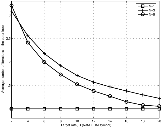
Figure 2: Average number of iterations in the outer loop required for the search of $\{k_{n}\}$

Fig. 2 shows the average iterations in the outer loop over $10^{3}$ independent channel realizations required for the search of $\{k_{n}\}$ to converge. It is shown that the average iteration numbers, denoted as $M$, is decreasing in $R$ and approaches $1$ when the target rate is sufficiently large. It can be explained by the fact that $k_{n}=K$ when $R$ goes infinity.

Since the binary search for $\mu$ in the inner loop involves $\log_{2}\left(\frac{\mu_{\max}-\mu_{\min}}{\varepsilon^{\prime\prime}}\right)$ iterations and finding $k_{n}$ for a given $R/\rho_{n}$ involves $\log_{2}(K)$ ones, the total number of iterations required for the IAS can be express as

$$C_{IAS}=M\left\{\log_{2}\left[\frac{\min_{n\in\mathcal{N}}\left(\frac{NR-k_{n}a_{n}}{k_{n}R}\right)-\max_{n\in\mathcal{N}}\left(\frac{1}{k_{n}}-\frac{a_{n}}{R}\right)}{\varepsilon^{\prime\prime}}\right]+N\log_{2}(K)\right\}$$ (43)

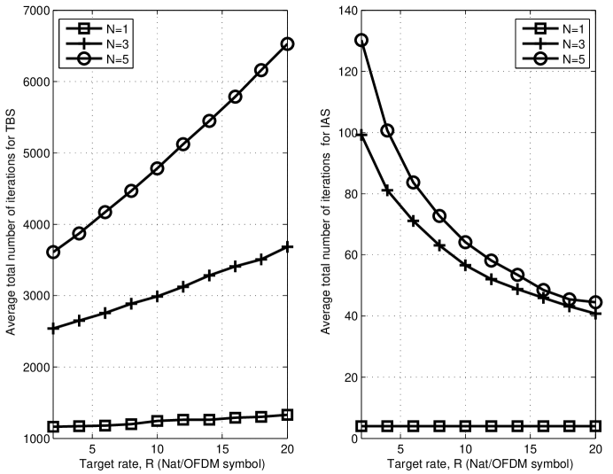
Figure 3: Average total number of iterations using TBS and IAS

Since $M$ is decreasing in $R$, $C_{IAS}$ is also decreasing in $R$ and upper bounded by a linear function of $N$. Fig. 3 compares average total complexities between TBS and IAS for different $R$ and different $N$.

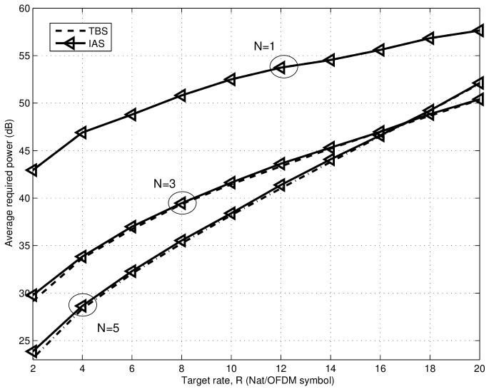
Figure 4: Average short-term power required to meet the target rate, $R$

Fig. 4 compares the average power required to meet the target rate between TBS developed in Section III-A1 and its sub-optimal algorithm, IAS. It is shown that IAS serves as a good approximation of TBS, especially for a high target rate.

As we discuss previously, the required controlling signals from the feedback channel are only geometric mean, harmonic mean of $g_{k,n}$ and the number of active subcarriers over each hop instead of $\{g_{k,n}~{},\forall k\in\mathcal{K},n\in\mathcal{N}\}$ as in TBS, thus the signalling exchange is greatly reduced when the number of subcarriers is large and/or the target rate is high. Furthermore, since IAS has low complexity and near-optimal power consumption performance, it is a good candidate for a sufficiently high target rate in a real system.

III-B Long-Term Power Threshold Determination

We have discussed the short-term total transmission power minimization. If the transmission is on for every possible channel realization, the long term power constraint may be violated. Similar to the single user case [10], the optimal power allocated to all hops for P1 with a long term power constraint must have the following structure,

$$p(\mathbf{g})=\left\{\begin{array}[]{ll}p_{\min}(\mathbf{g})&\mbox{with probability}~{}w(\mathbf{g})\\ 0&\mbox{with probability}~{}1-w(\mathbf{g})\end{array}\right..$$ (46)

Thus, the outage probability is $P(r(\mathbf{g},\mbox{\boldmath$\rho$},\mathbf{p})<R)=\mathbb{E}[1-w(\mathbf{g})]$. Then solving P1 is equivalent to finding the optimal weighting function $w(\mathbf{g})$ to the following problem,

$$\min_{w(\mathbf{g})} \mathbb{E}[1-w(\mathbf{g})]$$

s.t. $$0\leq w(\mathbf{g})\leq 1$$

$$\mathbb{E}[p_{\min}(\mathbf{g})w(\mathbf{g})]=P.$$

According to the result of [10, Lemma 3], the optimal weighting function has the form

$$w^{*}(\mathbf{g})=\left\{\begin{array}[]{ll}1&\mbox{for}~{}p_{\min}(\mathbf{g})<s^{*}\\ w_{0}&\mbox{for}~{}p_{\min}(\mathbf{g})=s^{*}\\ 0&\mbox{for}~{}p_{\min}(\mathbf{g})>s^{*}\end{array}\right..$$ (50)

The power threshold $s^{*}$ is given by $s^{*}=\sup\{s:\mathcal{P}(s)<P\},$ and $w_{0}$ is given by $w_{0}=\frac{P-\mathcal{P}(s^{*})}{\mathcal{\bar{P}}(s^{*})-\mathcal{P}(s^{*})},$ where the region $\mathcal{R}(s)$ and $\bar{\mathcal{R}}(s)$ are defined as $\mathcal{R}(s)=\{\mathbf{g}:p_{\min}(\mathbf{g})<s\},~{}\bar{\mathcal{R}}(s)=\{\mathbf{g}:p_{\min}(\mathbf{g})\leq s\},$ and the corresponding average power over the two sets are: $\mathcal{P}(s)=\mathbb{E}_{\mathbf{g}\in\mathcal{R}(s)}[p_{\min}(\mathbf{g})],\bar{\mathcal{P}}(s)=\mathbb{E}_{\mathbf{g}\in\bar{\mathcal{R}}(s)}[p_{\min}(\mathbf{g})]$ The resulting minimum outage probability is denoted as

$$P_{\rm{APT}}^{{out}}=1-\mbox{Prob}\{\mathbf{g}\in\mathcal{R}(s^{*})\}-w_{0}\mbox{Prob}\{p_{\min}(\mathbf{g})=s\}.$$

From (46) and (50), we see that when the minimum total power for all hops required to support the target transmission rate is beyond the threshold $s^{*}$, transmission is turned off. When the required power is less than the threshold, the transmission follows the minimum transmission power strategy derived from Section III-A.

The value of $s^{*}$ can be computed a priori if the fading statistics are known. Otherwise, the threshold can be estimated using fading samples. During the estimation of the threshold, since the channel is assumed to be ergodic, the ensemble average transmission power is equal to the time average

$$\mathbb{E}_{\mathbf{g}\in\mathcal{R}(s)}[p_{\min}(\mathbf{g})]=\lim_{t\rightarrow\infty}\frac{1}{t}\sum_{i=1}^{t}\hat{p}(i),$$

where $\hat{p}_{(i)}$ represents the actual transmission power at time frame $i$. Thus, the threshold is always adjusted in the opposite direction of $P-\frac{1}{t}\sum_{i=1}^{t}\hat{p}_{(i)}$ as

$$s^{*}(t+1)=s^{*}(t)\left[1+\epsilon\left(P-\frac{1}{t}\sum_{i=1}^{t}\hat{p}_{(i)}\right)\right].$$ (51)

where $t$ is the time frame index.

Combining the short-term power minimization and long-term power threshold determination, the full algorithm for APT is outlined as follows.

APT

1. Set $t=1$ and $s_{(t)}^{*}=P$

2. Search for minimum short-term power (developed in Section III-A)

3. On-off decision
   If $p_{\min}>s^{*}_{(t)}$, turn off the transmission and let $\hat{p}_{(t)}=0$; otherwise, turn on the transmission and let $\hat{p}_{(t)}=p_{\min}$.

4. Update the threshold $s^{*}$

   $$s^{*}(t+1)=s^{*}(t)\left[1+\epsilon\left(P-\frac{1}{t}\sum_{i=1}^{t}\hat{p}_{(i)}\right)\right].$$ (52)

5. Let $t=t+1$ and return to Step 1).

If TBS in Section III-A1 is used in Step 2), we name the optimal APT as APT-opt for short. If IAS in Section III-A2 is used, we denote it as APT-sub.

III-C Special case: adaptive power and fixed time allocation

APFT can be viewed as a special case of APT by fixing $\rho_{n}=1/N$. It can also be solved following two steps: short-term power minimization and long-term power threshold determination. However, unlike APT, the first step can be performed locally, i.e., each transmitter only needs to know the local CSI over the associated hop to solve the problem

$$\min_{\{p_{k,n}\}} \sum_{k\in\mathcal{K}}p_{k,n}$$

s.t. $$\frac{1}{N}\sum_{k\in\mathcal{K}}\ln(1+g_{k,n}p_{k,n})\geq R,$$

for all $n\in\mathcal{N}$. The solution of the problem is easily obtained as (25), where the water level is given by (29) with $\rho_{n}=1/N$.

IV Numerical results

In this section, we present some numerical results to illustrate the performance of the proposed adaptive power and time allocation for OFDM based linear relay networks. The proposed algorithms, APT-opt and APT-sub, are compared with UPT, FPAT and APFT as defined in Section II.

We consider an $N$-hop linear wireless network. The acceptable BER is chosen to be $10^{-5}$, which corresponds to 8.2dB SNR gap. We fix the bandwidth to be 1MHz and the end-to-end distance to be 1km. The relays are equally spaced. In all simulations, the channel over each hop is modelled by Stanford University Interim (SUI)-3 channel model with a central frequency at around 1.9 GHz to simulate the fixed broadband wireless access channel environments [19]. The SUI-3 channel is a 3-tap channel. The received signal fading on the first tap is characterized by a Ricean distribution with K-factor equal to 1. The fading on the other two taps follows a Rayleigh distribution. The root-mean-square (rms) delay spread is 0.305$\mu$s. Then the coherence bandwidth is approximately 65KHz. Hence, the number of subcarrier $K$ should be greater than 15.2 so that the subcarrier bandwidth is small enough to experience the flat fading. Here we choose $K=16$. Doppler maximal frequency is set to 0.4 Hz. Intermediate path loss condition ([20, Category B]) is chosen as the path loss model, which is given by $PL=A+\alpha\lg\left(\frac{d}{d_{n}}\right),$ where $A=20\lg(4\pi d_{0}/\lambda)$ ($\lambda$ being the wavelength in m), $\alpha$ is the path-loss exponent with $\alpha=(a-bh_{b}+c/h_{b})$. Here $h_{b}=30m$ is chosen as the height of the base station , $d_{0}=100m$ and $a$, $b$, $c$ are 4, 0.0065 and 17.1 given in [20]. The corresponding $\alpha$ will be used in all simulations except the one in Fig. 6. In each simulation, $10^{4}$ time frames are used to estimate the outage probability.

Fig. 5 shows the end-to-end outage probabilities versus average total transmission power for $R=1,20$ and 40 Nat/OFDM symbol using APT-opt when $N$ varies in the set of $\{1,3,5\}$. From the figure, it is shown that multi-hop transmission can help to save total power consumption when the target transmission rate is low (e.g., $R=1$) whereas it is better to send data directly to the destination if the target transmission rate is high (e.g., $R=40$). That can be explained by the following fact. As the number of hops increases, the path loss attenuation on each hop reduces. But the transmission time spent at each hop also reduces since the total frame length is fixed. It is observed from (2) that the transmission rate is linear in transmission time and concave in channel gain. Hence, when the target transmission rate increases, the loss due to transmission time reduction cannot be evened out by the gain brought by path loss reduction.

Fig. 6 shows the optimal number of hops to achieve minimum power consumption at different target transmission rates. Here, the outage probability is fixed to 1$\%$, and the path loss exponent $\alpha=$2.5 and 4, respectively. It is observed that the optimal number of hops is roughly proportional to the inverse of $R$, and increasing linearly in $\alpha$. A similar trend is shown in [21] where a spacial case, frequency-flat fading channel and a fixed short-term total power constraint, is considered.

Fig. 7 and Fig. 8 compare the end-to-end outage probabilities achieved by different power and time adaptation schemes for $R=1$ and $20$ Nat/OFDM symbols, respectively. A number of interesting observations can be made from the two figures. First, by comparing the curves of FPAT and UPT it is observed that just adapting per-hop transmission time alone can increase the performance considerably. But the decreasing speed of the outage probability as the total power increases is not increased much. On the other hand, by comparing the curves of APFT and UPT, it is seen that power adaption can bring dramatic improvement on the performance. In particular, the slope of the outage probability curves approaches almost infinity. This indicates that by turning off the transmission when the channel suffers from deep fade can achieve significant power saving. Next, comparing APT-opt with APFT we can see that time adaptation on top of power adaptation is still beneficial, but the gain is rather limited when the target data rate is small. Finally, it can be seen that the performance of APT-sub is even worse than that of APFT when the target rate is low (e.g. $R=1$). But for large target rate ($R=20$), APT-sub becomes superior and is near optimal.

The above numerical results suggest that multi-hop transmission is favorable at low and medium target rates, whereas a direct transmission from source to destination is preferred if the target rate is high. Also, power adaptation plays a more important rule than time adaptation in minimizing the end-to-end outage probability. In particular, APFT is a good choice in practice for low target rates since it has similar performance with APT-opt and yet is much less complex. For the similar reason, APT-sub is recommended at medium target rates.

V Conclusions

In this work, we consider adaptive power and time allocations for OFDM based linear relay networks for end-to-end outage probability minimization. The problem is solved in two steps. First, we derive the minimum short-term total power to meet the target transmission rate. Both optimal and sub-optimal algorithms are proposed. In particular, the sub-optimal algorithm suggests prolonging the transmission time for the hop with low geometric mean of channel gains averaged over subcarriers while lowering the transmission power for the hop with low harmonic mean. In the second step, the transmission on-off is determined by comparing the required minimum total power with a threshold, which is selected to satisfy the long-term total power constraint. Numerical study is carried out to illustrate the performance of different resource adaptation schemes: APT-opt, APT-sub, APFT, FPAT and UPT. We find that the three schemes with adaptive power control, APT-opt, APT-sub and APFT, provide significant power savings at a same end-to-end outage probability over the other two. While APFT is a good choice for practical implementation at low target rates, APT-sub becomes near optimal at medium target rats.

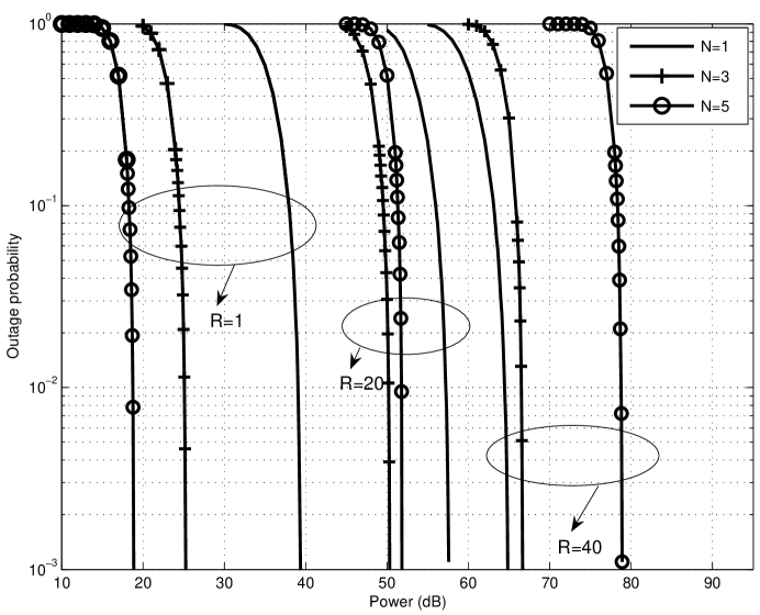
Figure 5: End-to-end outage probability vs. average total transmission power under APTA when $K=16$

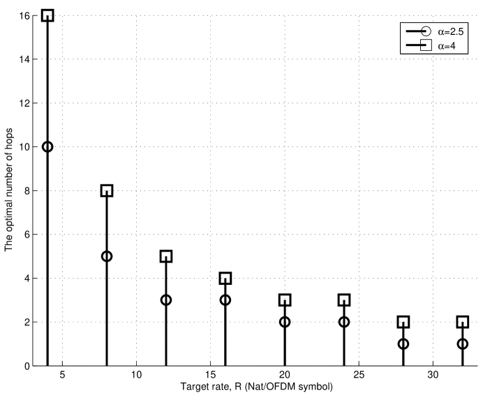
Figure 6: The optimal number of hops vs. target rate under APTA when $\alpha=2.5$ and 4

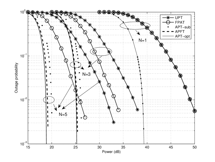
Figure 7: End-to-end outage probability vs. average total transmission power under APT-opt, APT-sub, APFT, FPAT and UPT when $K=16$ and $R=1$ Nat/OFDM symbol

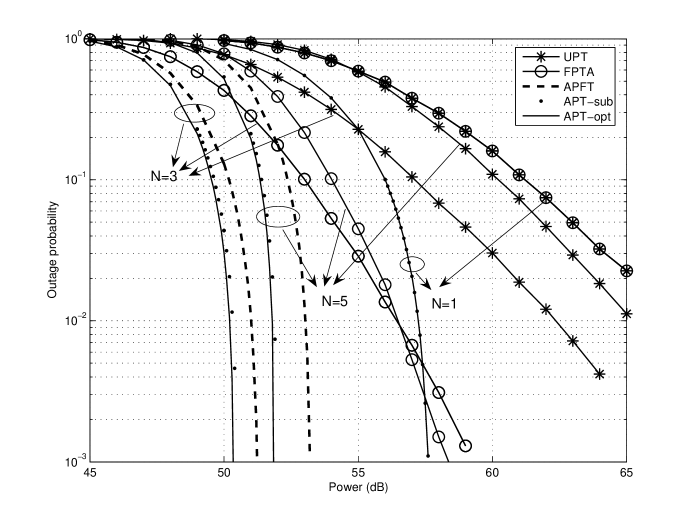
Figure 8: End-to-end outage probability vs. average total transmission power under APT-opt, APT-sub, APFT, FPAT and UPT when $K=16$ and $R=20$ Nat/OFDM symbol

References

- [1] R. Pabst, B. Walke, D. Schultz, P. Herhold, H. Yanikomeroglu, S. Mukherjee, H. Viswanathan, M. Lott, W. Zirwas, M. Dohler, H. Aghvami, D. Falconer, and G. Fettweis, “Relay-based deployment concepts for wireless and mobile broadband radio,” IEEE Commun. Mag., vol. 42, no. 9, pp. 80–89, 2004.
- [2] “Amendment to IEEE standard for local and metropolitan area networks - part 16: Air interface for fixed and mobile broadband wireless access systems - multihop relay specification,” March 2006. [Online]. Available: ieee802.org/16/relay/
- [3] Y. Yao, X. Cai, and G. Giannakis, “On energy efficiency and optimum resource allocation of relay transmissions in the low-power regime,” IEEE Trans. Wirel. Commun., vol. 4, no. 6, pp. 2917 – 2927, Nov. 2005.
- [4] M. Sikora, J. N. Laneman, M. Haenggi, J. Daniel J. Costello, and T. E. Fuja, “Bandwidth-and power-efficient routing in linear wireless networks,” IEEE Trans. Info. Theory, vol. 52, pp. 2624–1633, 2006.
- [5] O. Oyman, J. N. Laneman, and S. Sandhu, “Multihop relaying for broadband wireless mesh networks: From theory to practice,” IEEE Commun. Mag., vol. 45, no. 11, pp. 116–122, Nov. 2007.
- [6] B. Radunovic and J.-Y. L. Boudec, “Joint scheduling, power control and routing in symmetric, one-dimensional, multi-hop wireless networks,” in WiOpt, France, March 2003.
- [7] G. Li and H. Liu, “Resource allocation for OFDMA relay networks with fairness constraints,” IEEE J. Sel. Areas Commun., vol. 11, pp. 2061–2069, Nov. 2006.
- [8] L. Dai, B. Gui, and L. J. Cimini Jr., “Selective relaying in OFDM multihop cooperative networks,” in Proc. IEEE WCNC, Hong Kong, March 2007, pp. 963–968.
- [9] X. Zhang, W. Jiao, and M. Tao, “End-to-end resource allocation in OFDM based linear multi-hop networks,” in Proc. IEEE INFOCOM, Phoenix, AZ, USA, April 2008.
- [10] G. Caire, G. Taricco, and E. Biglieri, “Optimum power control over fading channelsl,” IEEE Trans. Info. Theory, vol. 45, no. 5, pp. 1468–1489, 1999.
- [11] L. Li and A. Goldsmith, “Capacity and optimal resource allocation for fading broadcast channels: Part II: outage capacity,” IEEE Trans. Info. Theory, vol. 47, no. 3, pp. 120–145, 2000.
- [12] J. N. Laneman, D. N. C. Tse, and G. W. Wornell, “Cooperative diversity in wireless networks: efficient protocols and outage behavior,” IEEE Trans. Info. Theory, vol. 50, pp. 3062–3080, 2004.
- [13] X. Qiu and K. Chawla, “On the performance of adaptive modulation in cellular systems,” IEEE Trans. Commun., vol. 47, no. 6, pp. 884–895, June 1999.
- [14] O. Oyman and S. Sandhu, “Non-ergodic power-bandwidth tradeoff in linear multi-hop networks,” in Proc. ISIT, Seattle, Washington, USA, July 2006.
- [15] S. Boyd and L. Vandenberghe, Convex Optimization. Cambridge, United Kingdom: Cambridge Univ. Press, 2004.
- [16] M. Tao, Y. Liang, and F. Zhang, “Adaptive resource allocation for delay differentiated traffics in multiuser ofdm systems,” accepted for publication in IEEE Trans. Wirel. Commun.
- [17] Y. Yao and G. B. Giannakis, “Energy-efficient scheduling for wireless sensor networks,” IEEE Trans. Commun., vol. 53, no. 8, pp. 1333–1342, Aug. 2005.
- [18] A. E. Gamal, C. Nair, B. Prabhakar, E. Uysal-Biyikoglu, and S. Zahedi, “Energy-efficient scheduling of packet transmissions over wireless networks,” in IEEE INFOCOM, New York, USA, March 2002.
- [19] V. Erceg, K. Hari, M. Smith, and D. Baum et al, “Channel models for fixed wireless applications,” IEEE 802.16.3c-01/29r1, 23 Feb 2001.
- [20] V. Erceg, L. Greenstein, S. Tjandra, S. Parkoff, A. Gupta, B. Kulic, A. Julius, and R. Jastrzab, “An empirically based path loss model for wireless channels insuburban environments,” IEEE J. Sel. Areas Commun., vol. 2, no. 11, pp. 1205–1211, 8-12 Nov. 1999.
- [21] M. Sikora, J. N. Laneman, M. Haenggi, J. D. J. Costello, and T. E. Fuja, “On the optimum number of hops in linear ad hoc networks,” in Proc. IEEE Info. Theory Workshop, San Antonio, Oct. 2004, pp. 165–169.