Microscopic theory of the Andreev gap

Abstract

We present a microscopic theory of the Andreev gap, i.e. the phenomenon that the density of states (DoS) of normal chaotic cavities attached to superconductors displays a hard gap centered around the Fermi energy. Our approach is based on a solution of the quantum Eilenberger equation in the regime $t_{D}\ll t_{\rm E}$, where $t_{D}$ and $t_{\mathrm{E}}$ are the classical dwell time and Ehrenfest-time, respectively. We show how quantum fluctuations eradicate the DoS at low energies and compute the profile of the gap to leading order in the parameter $t_{D}/t_{\rm E}$.

The attachment of a superconductor to a conducting cavity leads to a suppression of the normal density of states – the proximity effect. For cavities with classically chaotic dynamics, a discrepancy is found between semiclassical calculations prev and such based on random matrix theory (RMT) rmt : Semiclassics obtains a small yet finite DoS for all excitation energies $\epsilon$ above the Fermi level $\epsilon_{\rm F}$, while RMT predicts the formation of a hard gap below some energy $\epsilon^{\ast}$. The origin of this so-called ‘gap problem’ in Andreev billiards was pointed out by Lodder and Nazarov some time ago prev : quantum corrections not captured in the principal semiclassical approximation are expected to generate a hard spectral gap for trajectories longer than the Ehrenfest time. Although various semi-phenomenological realizations of this mechanism have been formulated, a fully microscopic theory of gap formation is outstanding. The construction of such a theory is the goal of the present paper.

Quasiclassical Eilenberger equation — Consider a two-dimensional Andreev billiard, i.e. a chaotic normal-conducting cavity attached to a bulk superconductor. We wish to compute the cavity DoS in a ‘semiclassical’ regime where the quantum time scales of the problem exceed all classical scales. Under these circumstances one expects prev the gap, $\epsilon^{\ast}$ to be set by the inverse of the Ehrenfest time, $\epsilon^{\ast}=\pi\hbar/2t_{\rm E}$, where $t_{\rm E}=\lambda^{-1}\ln(c^{2}/\hbar)$, $\lambda$ is the dominant Lyapunov exponent of the system, and $c^{2}$ a classical action scale whose detailed value is of little relevance. Heuristically, $t_{\rm E}$ is the time a minimal wave package needs to spread over classical portions of phase space; the dynamics at time scales beyond $t_{\rm E}$ is no longer classical.

To compute the DoS, we start out from the quantum Eilenberger equation (for notational convenience we suppress the infinitesimal imaginary increment in $\epsilon+i0$)

$$\left[\epsilon\sigma_{3}-i\Delta\sigma_{2}+H\openone\stackrel{{\scriptstyle\ast}}{{,}}G\right]=0$$ (1)

for the quasiclassical retarded matrix Green function, $G(\mathbb{x})$, i.e. the Wigner transform of the Gorkov superconductor Green function. In (1), $\sigma_{i}$ are Pauli matrices acting in particle-hole space, $\mathbb{x}=(\mathbb{q},\mathbb{p})^{T}$ is a phase space point in the shell of constant energy, $H(\mathbb{x})=\epsilon_{F}$, $H(\mathbb{x})$ is the Hamilton function, and the order parameter amplitude $\Delta=\Delta(\mathbb{q})$ is non-vanishing only at the cavity-superconductor interface. The Green function is subject to the nonlinear constraint $G\ast G=\openone$, and yields the DoS as $\nu(\epsilon)=\frac{\nu_{0}}{2\Omega}\operatorname{Re}\int d^{2}x\operatorname{tr}\left[G(\mathbb{x})\sigma_{3}\right]$, where $\Omega=\int_{H(\mathbb{x})=\epsilon_{F}}d^{2}x\,1$ is the volume of the energy shell and $\nu_{0}$ the normal metallic DoS. Finally, the symbol ‘$\ast$’ indicates that all products between phase space functions in Eq. (1) are Moyal products $(A\ast B)(\mathbb{x})=\exp\big{(}{i\hbar\over 2}\partial_{\mathbb{x^{\prime}}}^{T}I\partial_{\mathbb{x}}\big{)}\big{|}_{\mathbb{x}=\mathbb{x^{\prime}}}A(\mathbb{x^{\prime}})B(\mathbb{x})$.

Figure 1: Inset: classical trajectory connecting the superconductor/normal conductor interface of a chaotic Andreev billiard with itself. Main part: abstract phase space representation of that trajectory and its vicinity in a system of locally stable ($s$) and unstable ($u$) coordinates. The meaning of the shaded areas is explained in the main text.

Classical evolution and its inconsistency— Upon Taylor expansion to lowest orders $(A\ast B)(\mathbb{x})=A(\mathbb{x})B(\mathbb{x})+{i\hbar\over 2}\{A,B\}(\mathbb{x})+{\cal O}(\hbar^{2}\partial_{x}^{2})$ ($\{\,,\}$ is the Poisson bracket) Eq. (1) assumes the standard form of the classical Eilenberger equation eilenberger

$$[i\epsilon\sigma_{3}+\Delta\sigma_{2},G]-\hbar{\cal L}G=0,$$ (2)

where ${\cal L}=\{H,.\}$ generates the classical Liouville flow. However, (finite order) Taylor expansions of the Moyal product become problematic in cases where the function $G$ displays structure on linear scales $\lesssim{\cal O}(\hbar)$ and higher order derivatives ${\cal O}(\hbar^{2}\partial_{x}^{2})$ become of the same order as $\hbar{\cal L}$; as we shall see, this is precisely what happens on the solutions $G$ supporting the DoS in the region of the spectral gap.

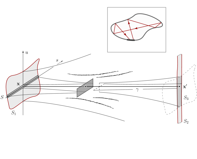
The classical Eilenberger equation (2) describes the evolution of $G$ along individual classical trajectories $\gamma$ beginning and ending at the superconductor interface (cf. inset of Fig. 1.) Parameterizing a trajectory $\gamma$ of length $T$ in terms of a coordinate $t\in[-T/2,T/2]$, the Liouville operator on $\gamma$ assumes the form ${\cal L}=\partial_{t}$ and the solution in the asymptotic limit $\epsilon/\Delta\rightarrow 0$ is prev

$$G_{T}(t)=-i\tan\left({\epsilon T\over\hbar}\right)\sigma_{3}+{\cos\left({2\epsilon t\over\hbar}\right)\sigma_{2}+\sin\left({2\epsilon t\over\hbar}\right)\sigma_{1}\over\cos\left({\epsilon T\over\hbar}\right)}.$$ (3)

Denoting the $\sigma_{i}$-components of $G$ by $G_{i}$, the solution obeys the boundary conditions prev

$$G_{T,1}(\pm T/2)=\pm iG_{T,3}(\pm T/2),\quad G_{T,2}(\pm T/2)=1.$$ (4)

The component $G_{T,3}=\mathrm{const.}$ generates (via the identity $\text{Im}\left(\tan\left(x+i0\right)\right)=\pi\sum_{m}\delta\left(x-(m+1/2)\pi\right)$) a quantization condition, $\epsilon T=(m+{1\over 2})\pi\hbar$, $m=0,1,2,...$, for the flight times of trajectories contributing to the DoS at energy $\epsilon$. The exponential sparsity of trajectories with $T\gg t_{\text{D}}$ much larger than the average dwell time pathdist then leads to an exponential suppression of the DoS for $\epsilon\lesssim\hbar t_{\text{D}}^{-1}$, but not to a gap.

In view of the continuity conditions underlying the approximation (2), it is mandatory to explore what happens as we transversally depart from an isolated trajectory into surrounding phase space. To this end, it is useful to interpret each trajectory as element of a corridor or band trbands1 ; effrmt ; trbands6 which is formed by all trajectories that run through the same sequence of scattering events. A schematic of a band is shown in the bottom part of Fig. 1, where the straight line represents a trajectory beginning and ending at points $\mathbb{x}$ and $\mathbb{x}^{\prime}$ in the SN interface. We introduce Poincaré sections through the trajectory, and span them by the locally stable and unstable coordinates, $s$ and $u$, respectively. The shaded areas then represent the SN interface ($S_{1}$), the image of that area under the Hamiltonian flow after time $t$ ($S_{2}$), the intersection of the image with the interface ($S_{3}$), and the pre-image of the intersection ($S$), respectively. Points in $S$ remain compactly confined and exit at the same instance $T$. The image of $S$ under evolution defines a ’corridor’ of sections across which the quasiclassical solutions $G_{T}$ is nearly constant. While the transverse area, $us$, of the corridor is a conserved quantity, its shape is not. At a given instance of time, $t$, its smallest linear extensions is given by (cf. Fig. 1) $\sim{\rm const.}\times{\,\rm min}(e^{-\lambda(T/2+t)},e^{{-\lambda(T/2-t)}})$, with a classical proportionality constant. For trajectory times $T>t_{\mathrm{E}}$, that scale may shrink below ${\cal O}(\hbar)$, and this is when Eq. (2) becomes problematic: at low energies, $\epsilon\sim\hbar t_{\rm E}^{-1}$, the narrow corridors of long trajectories $T>t_{\rm E}$ meander through the bulk of phase space, in which trajectories are of average length $\sim t_{\rm D}\ll t_{\rm E}$ and Green functions are ‘locked’ to the superconductor order parameter, $G(\epsilon)\simeq\sigma_{2}$. (Here and throughout, we use the notation $\simeq$ to indicate equality up to inconsequential corrections scaling with some positive power of $\hbar$.) The ensuing sharp variation of the solution $G_{T}$ over trans-corridor sections of quantum extension $\lesssim{\cal O}(\hbar)$ conflicts with quasiclassical smoothness conditions required for Eq. (2).

Our solution to the problem proceeds in two steps: we first transversally extend (3) to a solution of (2) in a ‘Planck tube’ fn11

$$Z=\bigcup_{-{T\over 2}\leq t\leq{T\over 2}}Z_{t},\quad Z_{t}=\{(u,s,t)|\;|us|\leq\hbar,\;|u|,|s|<c\},$$ (5)

centered around $\gamma$. This – singular – configuration will then be the basis for the construction of a smooth configuration $G$ that solves the quantum equation (1) up to corrections $\sim t_{D}/t_{\mathrm{E}}$. The quantum $G$ displays a hard spectral gap.

Figure 2: Vicinity of a long trajectory in a system of locally stable (s) and unstable (u) coordinates. Points at the boundary $|us|\sim\hbar$ belong to trajectories $\gamma$ generically of length $T\sim t_{\mathrm{E}}$ (here illustrated by the curved line.) The cloudy region at the ends of $\gamma$ represent generic phase-space points.

Consider, then, the corridor carried by a trajectory $\gamma$ of length $T\geq t_{\mathrm{E}}$. (In the wide corridors of shorter trajectories the Green function does not depend noticeably on transverse coordinates $(u,s,t)\in Z_{t}$ and the solution (3) can be taken face value.) We assume the corridor sections $Z_{t}$ to be small enough to afford a linearization ZurekPaz

$${\cal L}=\partial_{t}+\lambda u\partial_{u}-\lambda s\partial_{s},$$ (6)

where the terms $u\partial_{u}$ and $s\partial_{s}$ describe the divergence and contraction of phase flow around $\gamma$, respectively.

Figure 3: On the length of trajectories piercing the boundary of the Planck cell around a long reference trajectory. a) reference times corresponding to a bulk point in the N-region, b) point close to the exit into the superconductor, c) point close to the entrance into the N-region. Discussion, see text.

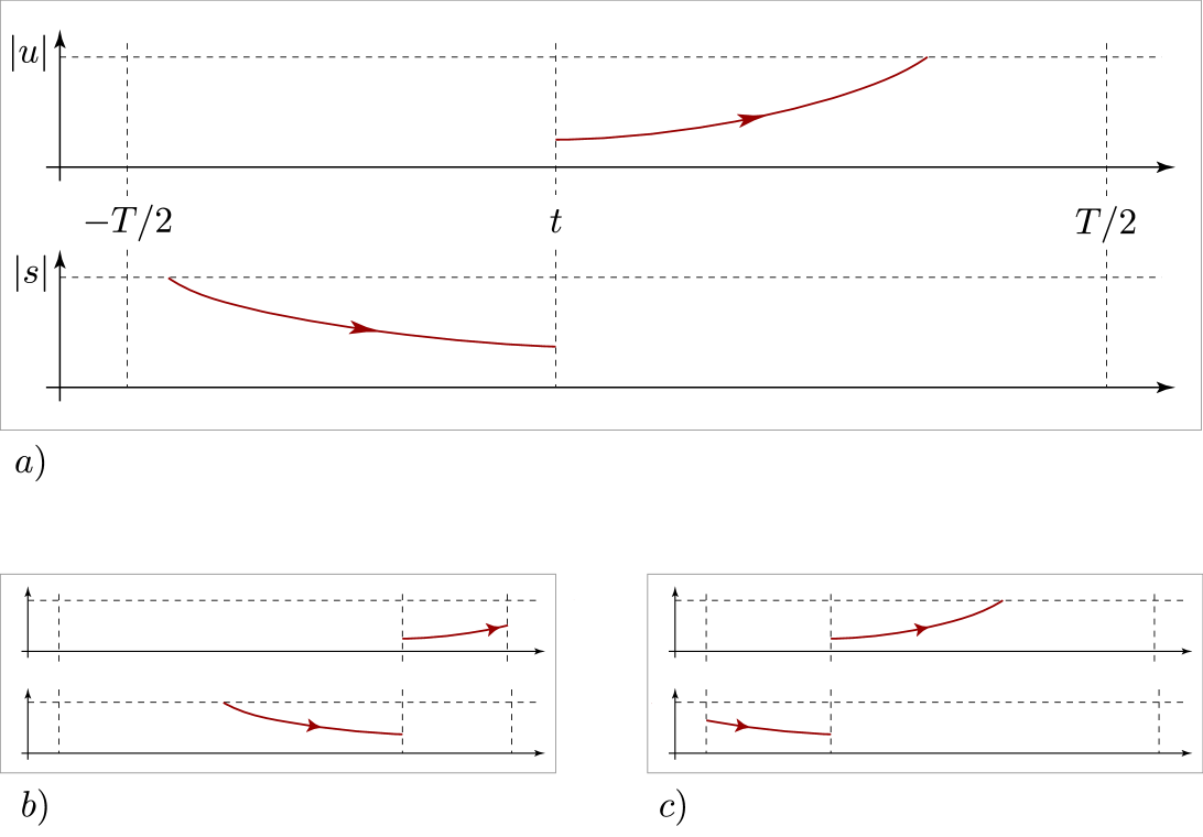
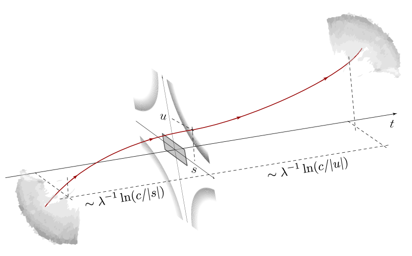
Going forward (backward) in time, the trajectory through a point $(u,s,t)\in Z_{t}$ will stay in the vicinity of $\gamma$ for a time $t(u)$ ($t(s)$) where $t(x)=\lambda^{-1}\ln(c/|x|)$. (cf. Fig. 2.) Thereafter a classically short time, typically of ${\cal O}(t_{\text{D}})$, passes before the departing trajectory exits; up to classical corrections, the time of flight of the trajectory through $(u,s,t)$ thus reads $t(u)+t(s)=\lambda^{-1}\ln(c^{2}/|us|)$. Specifically, for phase-space points on the boundary of the Planck cell $|us|\sim\hbar$ and therefore $t(u)+t(s)\simeq t_{\mathrm{E}}$. The above consideration applies to phase space points far away from the SN interface (cf. Fig. 3 a)). For points close to the interface, it may happen that the trajectory through $(u,s,t)$ hits the interface before it has diverged up to $c$, in which case the exit time is shorter than $t(u)$ (Fig. 3 b)). Or, it has been in the system for a time shorter than $t(s)$ before the reference point is reached (Fig. 3 c)). We subsume these different cases, by introducing effective in- and out-times $t_{o}(u)=\mathrm{min}(t(u),T/2-t)$ and $t_{i}(s)=\mathrm{min}(t(s),T/2+t)$, where the function $\mathrm{min}(t,t^{\prime})\equiv-{1\over\lambda}\ln\big{(}e^{-\lambda t}+e^{-\lambda t^{\prime}}\big{)}$ smoothly interpolates between $t$ and $t^{\prime}$ over a ‘microscopic’ switching interval $\sim\lambda^{-1}$. These functions evolve uniformly, in the sense ${\cal L}(t_{i/o}(s/u))=(+/-)1$. This means that the effective (up to corrections of ${\cal O}(t_{D}/t_{\textrm{E}})$) duration of the trajectory through $(u,s,t)\in Z_{t}$, is given by $T_{(u,s,t)}\equiv t_{o}(u)+t_{i}(s)$ and the trajectory parameter by $\tau_{(u,s,t)}\equiv{1\over 2}(t_{i}(s)-t_{o}(u))$. Substitution, $T\to T_{(u,s,t)}$ and $t\to\tau_{(u,s,t)}$ in (3) then obtains a transverse extension

$$G^{c}(u,s,t)\equiv G_{T_{(u,s,t)}}(\tau_{(u,s,t)})$$ (7)

of (2) fn_bound . $G^{c}$ solves the Eilenberger equation in direct consequence of the flow-uniformity of $t_{i}(s)$ and $t_{o}(u)$. By the same token, however, the solution becomes singular at times $T\geq t_{\mathrm{E}}$ when $t_{i,o}$ begin to display structure on scales $\lesssim\hbar$. Next, we show that this is not what happens in the full quantum dynamics.

Quantum evolution and spectral gap— Let us define a generalization, $t^{q}_{i}(u,s,t)$, of $t_{i}(s,t)$ by requiring uniformity under the full dynamics, $-i\hbar^{-1}[H\overset{\ast}{,}\,t_{i}^{q}]=1$, or

$${\cal L}\,t_{i}^{q}+[{\cal V}\overset{\ast}{,}\,t_{i}^{q}]=1,$$ (8)

where $[{\cal V}\overset{\ast}{,}\;]\equiv-i\hbar^{-1}[H\overset{\ast}{,}\;]-{\cal L}$ accounts for quantum corrections to the linearized classical dynamics. The above equation may be solved by introducing ‘action-angle coordinates’ $I=us$, $\phi\equiv{1\over 2}\ln(u/s)$ in terms of which ${\cal L}=\partial_{t}+\lambda\partial_{\phi}$. The ${\cal V}$-term may now be formally removed by ‘gauging’ Eq. (8) with

$$U(I,\phi,t)={\cal P}e_{\ast}^{{1\over\lambda}\int_{0}^{\phi}d\phi^{\prime}{\cal V}(I,\phi^{\prime})},$$ (9)

where $e_{\ast}^{(...)}$ is defined by a Moyal series expansion in the exponent and ${\cal P}$ is a $\phi$-ordering prescription (see Ref. [wl1, ] for details) accounting for the non-commutativity of ${\cal V}(I,\phi)$ at different values of $\phi$. By construction [wl2, ], $U$ obeys ${\cal L}U={\cal V}\ast U$, which means that Eq. (8) is solved by

$$t^{q}_{i}(u,s,t)=(U\ast t_{i}\ast U^{-1})(u,s,t).$$ (10)

In practice, both the detailed form of ${\cal V}$ and of $U$ will not be known. This lack of knowledge, however, is not of essential concern to us; to the logarithmic accuracy required by the present analysis, basic scaling arguments suffice to determine the action of $U$ on $t_{i}$: describing nonlinear corrections to the flow, the expansion of ${\cal V}$ for small $u,s$ starts as $\hbar{\cal V}=us\times{\cal O}(u^{n}s^{m}),n+m>0$. Accordingly, $U=1+\hbar^{-1}us\times{\cal O}(u^{n}s^{m})$. This entails that for any function $f$ that is smooth (analytic) around $u=s=0$, $(U*f*U^{-1})(u,s)=f(u,s)+{\cal O}(\partial_{u}fu^{n+1}s^{m},\partial_{s}fu^{n}s^{m+1})$. At the small values of coordinates we are interested in, $|us|\sim\hbar$, the ${\cal O}(\dots)$-terms become irrelevant, which reflects the irrelevancy of dynamical corrections to the linearized flow close to the trajectory center. To explore the effect of $U$ on singular functions (such as $t_{i}(s)\sim\ln(|s|)$), we notice that for arbitrary $f(s)$,

$$e^{-iku}\ast f(s)=f(s+\hbar k)\ast e^{-iku}.$$ (11)

This identity suggests to introduce a Fourier mode decomposition $U(u,s,t)=\int dk\,U_{(s,t)}(k)e^{-iku}$. Specifically, let us consider values $|s|\sim\hbar$, where singularities begin to put the semiclassical theory at risk. For these values, the support of the mode coefficients $U_{(s,t)}(k)$ extends up to ’classical’ values $k\sim\hbar^{0}$ fn_ucl . We thus obtain $t_{i}^{q}(u,s,t)=\int dk\,t_{i}(s+\hbar k)\ast F_{(s,t)}(k)$, where the positive indefinite but normalized ($\int dkF_{(s,t)}(k)=1$) ‘weight’ function $F_{s}(k)=\left(e^{-iku}U_{(s,t)}(k)\right)\ast U^{-1}(u,s,t)$. A straightforward estimate now shows that for asymptotically small $\hbar$ the integral evaluates to $t_{i}^{q}(u,s,t)=t_{i}(|s|+\hbar/u_{0})\simeq\mathrm{min}(t_{i}(s),t_{\mathrm{E}})$, where $u_{0}$ is a non-universal constant. Similarly, $t^{q}_{o}(u,s,t)\simeq\mathrm{min}(t_{o}(u),t_{\mathrm{E}})$. Summarizing, we have found that the operators $U$ act to truncate singularities in trajectory times in a manner independent of the detailed form of the potential ${\cal V}$.

Building on these results it is now straightforward to construct a smooth solution of the quantum equation (1): its general solution is given by $C\sigma_{3}+(1-C^{2})\left(\cos\left({\epsilon\tau^{q}\over\hbar}\right)\sigma_{2}+\sin\left({\epsilon\tau^{q}\over\hbar}\right)\sigma_{1}\right)$, where $\tau^{q}=(t^{q}_{i}-t^{q}_{o})/2$ and we used that smooth functions $f(\tau^{q})$ (’$\sin$’, ’$\cos$’, etc.) evolve linearly, $[H\overset{\ast}{,}\,f(\tau^{q})]\simeq f^{\prime}(\tau^{q})[H\overset{\ast}{,}\,\tau^{q}]=i\hbar f^{\prime}(\tau^{q})$, up to corrections of ${\cal O}(1/t_{\rm E}\lambda)$ fn_tel . The normalization function $C=C(u,s,t)$ is determined by requiring stationarity $[H\overset{\ast}{,}\,C]=0$, and compatibility with the boundary conditions (4). These two conditions lead to the identification $C=i\tan(\epsilon T^{q}(u,s,t)/\hbar)$, where $T^{q}(u,s,t)=\min(T(u,s,t),t_{\mathrm{E}})$ is the effective trajectory time. In conclusion, we have found that the quantum equation (1) is solved by $G_{T^{q}(u,s,t)}(\tau^{q}(u,s,t))$, which differs from the solution of the classical equation (2) by an upper cutoff $t_{\mathrm{E}}$ limiting both the trajectory time $T^{q}$ and the trajectory parameter $\tau^{q}$. Technically, this is the main result of the present letter.

The above solution signals that quantum fluctuations couple narrow bands of transverse extension $\lesssim\hbar$ to neighboring phase space. This coupling is strongest in the terminal regions of long trajectories $|\tau|\gtrsim t_{\mathrm{E}}$ where bands flatten in one direction. Inspection of Fig. 2 shows that the $\hbar$-neighborhood of these segments is pierced by trajectories whose length and parameter are uniformly given by $T\simeq t_{\mathrm{E}}$ and $|\tau|\simeq t_{\mathrm{E}}/2$, respectively. At these values the solutions $G$ are nearly stationary (up to corrections ${\cal O}(t_{D}/t_{\mathrm{E}})$, and this reflects in the asymptotic constancy of the regularized solution $G_{T^{q}\gtrsim t_{\mathrm{E}}}(\tau^{q}\gtrsim\pm t_{\mathrm{E}})\simeq G_{t_{\mathrm{E}}}(\pm t_{\mathrm{E}})$ at large parameter values. The capping of trajectory times $T^{q}\lesssim t_{\mathrm{E}}$ in turn implies a vanishing of the DoS for energies $\epsilon<\epsilon^{\ast}$. (Technically, $\mathrm{Re}(G_{3}(\mathbb{x}))=-\mathrm{Im}\tan(\epsilon T^{q}(u,s,t)/\hbar)$ is vanishing for these energies.) The fact that all trajectories of nominal length $T>t_{\mathrm{E}}$ get reduced to the uniform effective length $T^{q}\simeq t_{\mathrm{E}}$ implies an accumulation of spectral weight at the gap edge $\epsilon^{\ast}=\pi\hbar/2t_{\mathrm{E}}$. A straightforward estimate based on the classical density of long trajectories $p(T)dT\sim\exp(-T/t_{\mathrm{D}})dT$ shows that the peak is of moderate height $\rho(\epsilon^{\ast})/\rho_{\mathrm{cl}}(\epsilon^{\ast})={\cal O}(1)$, where $\rho_{\mathrm{cl}}(\epsilon^{\ast})$ is the semiclassical estimate of the DoS. Its width is of ${\cal O}(t_{\mathrm{D}}/t_{\mathrm{E}}^{2})$ which reflects an uncertainty in the effective trajectory times of ${\cal O}(t_{\mathrm{D}})$. In a real environment, the position of the gap may also be affected by mesoscopic fluctuations of system parameters silvestrov . However, such effects are beyond the scope of the present paper.

Summary and discussion — We have solved the quantum Eilenberger equation to leading order in the small parameter $t_{D}/t_{E}$. Our solution verifies the existence of a gap in the DoS of clean chaotic Andreev billiards. It is worthwhile to compare these results to two earlier approaches to dealing with the singularities of the classical Eilenberger theory: in [effrmt, ], Silvestrov et al. argued that on bands narrower than a Planck cell, classical dynamics may be effectively replaced by RMT modeling. In [vavlarkin, ] Vavilov and Larkin, coupled the system to artificial short range disorder, fine tuned in strength to mimic quantum corrections to classical propagation. This latter procedure renders the long time dynamics effectively stochastic, thus preventing the build-up of sharply defined phase space structures. Our analysis shows that phenomenological input of either type is not, in fact, necessary. The conjunction of classical hyperbolicity and quantum uncertainty encoded in the native Eilenberger equation automatically regularizes classical singularities at large times. This mechanism operates under rather general conditions and can be described at moderate theoretical efforts. We therefore believe the concepts discussed above to be of wider applicability.

We are grateful for discussions with P. Brouwer. This work was supported by SFB/TR 12 of the Deutsche Forschungsgemeinschaft and the U.S. Department of Energy, Office of Science, under Contract No. DE-AC02-06CH11357.

References

- (1) A. Lodder, Y. V. Nazarov, Phys. Rev. B 58, 5783 (1998).
- (2) J. Melsen et al., Europhys. Lett. 35, 7 (1996).
- (3) G. Eilenberger, Z. Phys. 214, 195 (1968); J. Rammer, Quantum Field Theory of Non-Equilibrium States (Cambridge, New York, 2007).
- (4) The distribution of path lengths in chaotic billiards is dt .
- (5) W. Bauer et al., Phys. Rev. Lett. 65, 2213 (1990).
- (6) L. Wirtz et al., Phy. Rev. B, 56, 7589 (1997).
- (7) P. G. Silvestrov et al., Phys. Rev. Lett. 90, 116801 (2003).
- (8) R. S. Whitney et al. , Phys. Rev. Lett. 94, 116801 (2005).
- (9) The principal role of the Planck cell in this context has already been discussed in H. Schomerus and C. W. J. Beenakker, Phys. Rev. Lett. 82, 2951 (1999).
- (10) W. H. Zurek, J. P. Paz, Phys. Rev. Lett. 72, 2508 (1994).
- (11) D. J. Gross et al., Adv. Theor. Math. Phys. 4, 893 (2000).
- (12) At its terminal points, respects the boundary conditions (4). This is because at the trajectory has either hit the superconductor interface (Fig. 3 b,c)), or they have left the vicinity of the reference trajectory (Fig. 3 a)), meaning that they will hit the interface after a classically short time .
- (13) A detail proof of this property can be found in Appendix A of M. Chaichian et al., Phys. Lett. B 666, 199 (2008).
- (14) The (super)linear scaling of in implies that as a function of , . By the same token, the -dependence of the function is classical, and the same applies to the mode spectrum.
- (15) This is seen by straightforward comparison of the action of the Moyal product’s higher order derivatives on the envelope function and its argument function , resp.
- (16) P. G. Silvestrov, Phys. Rev. Lett. 97, 067004 (2006).
- (17) M. G. Vavilov, A. I. Larkin, Phys. Rev. B 67, 115335 (2003).