Harmonic moment dynamics in Laplacian growth

Abstract

Harmonic moments are integrals of integer powers of $z=x+iy$ over a domain. Here the domain is an exterior of a bubble of air growing in an oil layer between two horizontal closely spaced plates. Harmonic moments are a natural basis for such Laplacian growth phenomena because, unlike other representations, these moments linearize the zero surface tension problem (Richardson, 1972), so that all moments except the lowest one are conserved in time. For non-zero surface tension, we show that the the harmonic moments decay in time rather than exhibiting the divergences of other representations. Our laboratory observations confirm the theoretical predictions and demonstrate that an interface dynamics description in terms of harmonic moments is physically realizable and robust. In addition, by extending the theory to include surface tension, we obtain from measurements of the time evolution of the harmonic moments a value for the surface tension that is within 20% of the accepted value.

I INTRODUCTION

I.1 Laplacian growth and viscous fingering

Non-equilibrium processes give rise to a variety of patterns with remarkable geometrical and dynamical properties Cross and Hohenberg (1993); Gollub and Langer (1999). Often these processes are represented by the dynamics of an unstable interface between different phases, and the interface patterns can exhibit universal features Pelcé (1988). Examples include crack propagation Gollub and Langer (1999), fluid-fluid interface dynamics Saffman and Taylor (1958), crystal formation Langer (1980), and biological growth Ben-Jacob (1997).

The simplest process leading to unstable universal patterns is Laplacian growth, where the velocity of an interface is proportional to the gradient of function that is harmonic outside (or inside) the interface. Here we examine the simplest example of Laplacian growth: quasi-two-dimensional (2D) viscous fingering in a Hele-Shaw cell Hele-Shaw (1898), where a viscous fluid is displaced by an inviscid fluid between two horizontal closely spaced parallel plates.

Figure 1 shows four viscous fingering patterns grown in the radial Hele-Shaw cell described in Section IV. Viscous silicone oil is removed from a buffer surrounding the plates and air enters between the plates through a central hole in the bottom plate.

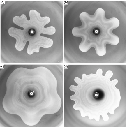
Figure 1: Viscous fingering patterns of air in oil contained between two plates separated by 125 $\mu$m (image size is 14 cm $\times$ 14 cm) (a) Bubble grown at a constant pumping rate of 0.52 mL/min. (b), (c), (d) Bubbles grown with varying pumping rates, as described in Section IV.B. The time development of bubble (b) is shown in Fig. 3.

As the air bubble expands, the oil/air interface is unstable. The depth averaged velocity ${\bf v}(x,y)$ and the pressure $p(x,y)$ in the oil are approximated by Darcy’s law Lamb (1945)

$${\bf v}=-\frac{b^{2}}{12\mu}\nabla p\,,$$ (1)

where $b$ is the spacing between the plates and $\mu$ is the dynamic oil viscosity. The oil is incompressible, so ${\rm div}\,{\bf v}=0$. From (1) it then follows that in the oil

$$\nabla^{2}p=0\,.$$ (2)

Since the normal velocities of the interface $V$ and of the fluid at the interface coincide Lamb (1945),

$$V=-\frac{b^{2}}{12\mu}\partial_{n}p\,,$$ (3)

where $\partial_{n}$ is the normal component of the gradient. Because the air is nearly inviscid, the pressure in the air is essentially uniform, and its value can be taken as zero. Thus the pressure jump across the oil/air interface coincides with the oil pressure at the interface and is given by Saffman and Taylor (1958)

$$p=-\sigma\kappa\,,$$ (4)

where $\sigma$ is surface tension and $\kappa$ is the local curvature of the interface in the horizontal plane. (An updated boundary condition including a $\pi/4$ multiplicative factor and an additional term correcting for wetting will be presented in Section III.2.)

The asymptotic pressure boundary condition in oil far from the interface in the radial geometry is

$$p=-\frac{3\mu Q}{\pi b^{2}}\log(x^{2}+y^{2})\qquad({\rm for}\,\,x^{2}+y^{2}\rightarrow\infty),$$ (5)

where $Q$ is the pumping rate (the rate of area growth), which may depend on time. Equations (1)-(5) complete the description of 2D viscous fingering, which is a prototype of Laplacian growth.

Laplacian growth, a classical free-boundary problem Gillow and Howison (1998), is famous in both physics and mathematics: In physics, because the process is highly unstable, dissipative, non-equilibrium, and nonlinear, and because the growth produces universal patterns Saffman and Taylor (1958); Ristroph et al. (2006); Segur et al. (1991). In mathematics, because the description (1)-(5), as simple as it looks, reveals a powerful and profound structure Mineev-Weinstein et al. (2000); Krichever et al. (2004); Mineev-Weinstein et al. (2008).

Laplacian growth occurs in many physical systems and is known by names such as crystal growth, amorphous solidification Langer (1980), electrodeposition Ciliberto and Gollub (1984); Sawada et al. (1986), bacterial colony growth Ben-Jacob (1997), diffusion-limited aggregation (DLA) Witten and Sander (1981), motion of a charged surface in liquid Helium Zubarev (2002), and viscous fingering Praud and Swinney (2005). There are thousands of articles (theoretical, experimental, and computational) devoted to Laplacian growth if one includes work on closely connected problems such as the Stefan problem (solidification) Kessler et al. (1988); Langer and Muller-Krumbhaar (1978), DLA Halsey (2000), and the phase-field model Gollub and Langer (1999). Nevertheless, many features remain unexplained, despite extensive effort and full knowledge of the laws of physics describing the process.

I.2 Harmonic Moments

The present work concerns a powerful description of Laplacian growth called harmonic moments. Our work demonstrates that robust results for the time evolution of harmonic moments can be obtained from viscous fingering data. Harmonic moments are defined as

$$M_{k}=\int_{D}z^{-k}\,\frac{dxdy}{\pi}=-\oint_{\Gamma}z^{-k}\,\overline{z}\,\frac{\,dz}{2\pi i},$$ (6)

where $k=0,1,\ldots,\infty$, $z=x+iy$, and the domain of integration $D$ is exterior to a pattern’s boundary $\Gamma$ and bounded by a large circle on the outside. These are exterior moments, which are relevant for exterior Laplacian growth, when a viscous fluid is outside the interface, as in this work. Interior moments, which are relevant for interior Laplacian growth when a viscous fluid is inside the interface, are defined similarly, but with positive powers of $z$ under the integral, which is taken over the interior of the pattern.

Harmonic moments are of fundamental importance for Laplacian growth because in the absence of surface tension, there is an infinite number of conservation laws: all moments $M_{k}$ (except for $k$ = 0) are conserved in time, as was discovered by Richardson (1972) Richardson (1972) for the interior Laplacian growth problem. The conservation laws have been extended to the exterior case Mineev (1990) and are experimentally confirmed in this work. In the harmonic moments basis the whole evolution of $D(t)$ is reduced to the time-dependent area of a growing bubble, which is $M_{0}(t)$. This result selects the ‘harmonic basis’ $M_{k}$ from all other bases as the best basis for describing $D(t)$ in Laplacian growth.

Harmonic moments form a complete basis for representing any 2D interface, regardless of its complicated shape, provided that $D$ is analytic and singly connected Novikoff (1938); Etingof and Varchenko (1992). Like Fourier modes, each harmonic moment $M_{k}$ corresponds to a particular aspect of the interface. The moment $M_{0}$ is the area of the domain $D$ divided by $\pi$. Moments $M_{k}$ for $k\geq 1$ are proportional to the amplitude of a monochromatic wave, which modulates the circle with an exactly $k$ waves along the circumference,

$$z=R\,\exp(i\phi)[1+a_{k}\,\,exp(-ik\phi)],$$

where $\phi$ is a ‘stream function’ parameter along the interface, $a_{k}$ is an amplitude, and $R$ is the bubble radius. Specifically, $M_{k}=a_{k}\,R^{2-k}$. For an approximately $n$-fold pattern, the dominant moments are $M_{n}$, $M_{2n}$, $M_{3n}$, etc. [e.g. Fig. 1(b) is approximately 7-fold symmetric and Fig. 1(c) is approximately 5-fold symmetric]. However, care should be taken in comparing different moments since they have different units; the moment $M_{k}$ has units cm^2-k.

Viscous fingering structures become extremely complex for high growth rates, where tips repeatedly split and form new fingers and fjords. Hence it is remarkable that theory predicts that a set of purely geometrical quantities, $M_{k}$, will change slowly during the growth process and will have a well-defined limit as the surface tension approaches zero. The unique properties of harmonic moments have been already used to establish connections between Laplacian growth and other fields of physics and mathematics Mineev-Weinstein et al. (2000); Krichever et al. (2004); Mineev-Weinstein et al. (2008), but no previous studies have attempted to extract harmonic moments from laboratory data. Our work demonstrates that robust moments $M_{k}$ can indeed be obtained from experiments, and particularly that the moments $M_{k}$ for $k\geq 1$ are conserved in the limit of zero surface tension.

I.3 Overview

In the following section we present some additional properties of harmonic moments. Section III extends the theory for harmonic moments in viscous fingering to the physical case, where the surface tension is not zero. In this case, the moments $M_{k}$ with positive $k$ are no longer conserved, but their time derivatives are proportional to surface tension and hence vanish in the zero surface tension limit. Section IV presents our experimental and data analysis methods. Section V presents results for harmonic moments determined from experiments for a wide range of conditions. Also we show that the results for the harmonic moments can be used to deduce a physical parameter, such as surface tension. Section VI discusses the significance of our results.

II HARMONIC MOMENTS: HISTORY AND APPLICATIONS

II.1 The Inverse Potential Problem

The origin of harmonic moments dates back to Isaac Newton’s study of the Inverse Potential Problem, which was subsequently investigated by Kelvin, Poincaré and many researchers in the twentieth century. The Inverse Potential Problem Novikoff (1938); Etingof and Varchenko (1992) asks how to recover the shape of a domain occupied by a uniformly distributed mass, given the gravitational potential created by this mass outside the domain. Surprisingly, this classical mathematical problem was found to be at the heart of the underlying mathematical structure of Laplacian growth Richardson (1972); Mineev-Weinstein et al. (2000); Krichever et al. (2004); Mineev-Weinstein et al. (2008). In two dimensions the gravitational potential created by uniformly distributed mass (with unit density) occupying the domain $D$ is given by

$$\Phi(x,y)=\frac{1}{\pi}\int_{D}\,\log|z-z^{\prime}|\,dx^{\prime}dy^{\prime}=$$

$$\frac{1}{\pi}\int_{D}\,\log|z^{\prime}|\,dx^{\prime}dy^{\prime}-{\cal R}e\sum_{k=1}^{\infty}M_{k}z^{k}/k,$$ (7)

if $z$ and the origin lie outside $D$. The $M_{k}$, defined in (6), are multipole moments of the mass distribution Jackson (1999). In Laplacian growth the $M_{k}$ are traditionally called harmonic moments. In (6) the moments $M_{k}$ are defined for a radial geometry. For a rectangular geometry, where matter occupies a horizontal semi-infinite strip $D$ with a width $L$ bounded from the left by an arbitrary curve, and periodically extended (repeated) both up and down infinitely, the moments are defined as $M_{k}=\int_{D}\exp(-2\pi kz/L)\,dxdy/\pi$. This geometry is relevant for Laplacian growth in a rectangular Hele-Shaw channel, which has been studied since the work by Saffman and Taylor Saffman and Taylor (1958).

II.2 Connections and Applications

In science and engineering it is often of interest to find the shape of an object from the indirect measurement of the harmonic moments $M_{k}$. The problem of domain reconstruction from its moments has applications in many areas, including signal processing, probability and statistics, tomography, and the inverse potential problem in geophysics (magnetic and gravitational anomaly detection) Landau (1987). While the recovery of shapes from moments is often an ill-posed problem, it was recently recognized that the moments problem allows the complete closed form solution for so-called quadrature domains Gustafsson and Putinar (2007), a branch of mathematics created in 1970s Aharonov and Shapiro (1976); Sakai (1982). Remarkably, these solutions are based on a technique of numerical linear algebra that yields numerically stable and fast algorithms and exposes a deep connection between harmonic moments and a theory of analytic approximation Golub et al. (1999); Gustafsson et al. (2000).

III THEORY OF HARMONIC MOMENTS WITH NONZERO SURFACE TENSION

III.1 Derivation of $dM_{k}/dt$

In Laplacian growth with nonzero surface tension the harmonic moments are no longer conserved. To relate the dynamics of the harmonic moments to measurable quantities in viscous fingering, we now obtain an expression for the time derivative of the harmonic moments in terms of a line integral over the air/oil interface. The time derivative of $M_{k}$ follows from the definition (6) and (1):

$$\frac{dM_{k}}{dt}=\frac{b^{2}}{12\mu}\oint_{\Gamma}z^{-k}\,\partial_{n}p\,\frac{\,dl}{\pi}=$$

We want to exchange the derivative between $p$ and $z^{-k}$, so we add and subtract $p\,\partial_{n}z^{-k}$ from the integrand,

$$=\frac{b^{2}}{12\mu}\oint_{\Gamma}(z^{-k}\,\partial_{n}p-p\,\partial_{n}z^{-k}+p\,\partial_{n}z^{-k})\,\frac{\,dl}{\pi}.$$ (8)

Here $l$ is the arc length along the interface $\Gamma$. The integral of the first two terms is zero by Gauss’s theorem, after using (3) and the analyticity of $z^{-k}$ in $D$,

$$\oint_{\Gamma}(z^{-k}\,\partial_{n}p-p\,\partial_{n}z^{-k})dl=\oint_{\Gamma}(z^{-k}\nabla p-p\nabla z^{-k})\cdot\vec{n}\,dl$$

$$=\int_{D}\nabla\cdot(z^{-k}\nabla p-p\nabla z^{-k})\,dx\,dy=0.$$ (9)

Using (4) for the pressure, we have

$$\frac{dM_{k}}{dt}=-\frac{\sigma b^{2}}{12\pi\mu}\oint_{\Gamma}\kappa\,\,\partial_{n}\,z^{-k}\,dl$$ (10)

with the interfacial curvature given by $\kappa=d\theta/dl$, where $\theta$ is the angle of a tangent line to the interface. Using the identity $\partial_{n}\,z^{-k}=i\partial_{l}z^{-k}$ = $-ikz^{-(k+1)}dz/dl$, where $\partial_{l}$ denotes a tangential derivative, we have

$$-\frac{\sigma b^{2}i}{12\pi\mu}\oint_{\Gamma}\frac{d\theta}{dl}\,\,\partial_{l}\,z^{-k}\,dl=\frac{k\sigma b^{2}i}{12\pi\mu}\oint_{\Gamma}\,\,z^{-(k+1)}\,\frac{dz}{dl}\,\,d\theta$$

$$=\frac{k\sigma b^{2}}{12\pi\mu}\oint_{\Gamma}\,\,z^{-(k+1)}\,d\,e^{i\theta}.$$ (11)

where the last expression was obtained using $dz/dl=\exp(i\theta)$. Integrating by parts, we obtain

$$\frac{dM_{k}}{dt}=\sigma\,k(k+1)\,\frac{b^{2}}{12\pi\mu}\oint_{\Gamma}\,e^{i\theta}\,\frac{\mathrm{d}z}{z^{k+2}}.$$ (12)

Note that Richardson’s result for the conservation of moments is recovered in the limit that the surface tension $\sigma$ vanishes. Surface tension is now a regular rather than a singular perturbation.

III.2 Wetting and scaling correction

The pressure jump at the interface (4) must be modified because as the air bubble advances between the glass plates, it leaves behind a wetting film on each plate. The thickness of this film increases with the interface’s velocity Park and Homsy (1984). This film can be seen as interference fringes on the images in Fig. 1, because the interface is slowing down as the bubble expands. In addition, a factor $\pi/4$ is needed in (4). The pressure jump including the wetting correction and a factor $\pi/4$ [not in (4)] was calculated by Park and Homsy to be Park and Homsy (1984),

$$p=-\sigma\left(\frac{\pi\kappa}{4}\right)+\frac{2\sigma}{b}\left[1+3.8\left(\frac{\mu V}{\sigma}\right)^{2/3}\right],$$ (13)

where $V$ is the local normal velocity of the interface. The thickness of the film predicted by Park and Homsy was experimentally confirmed by Tabeling and Libchaber Tabeling and Libchaber (1986) for $6\times 10^{-4}<\frac{\mu V}{\sigma}<3\times 10^{-3}$.

The interface velocity $V$ is greatest at the finger tips and is much smaller at the sides of the fingers. Conventionally the base of the fjord is called a stagnation point, although in these experiments there is small motion at the base of the fjords as a consequence of relaxation due to surface tension; the base of the fjord becomes more bulbous the longer surface tension has acted on it.

After substituting this new expression for the pressure jump into (10), we obtain

$$\frac{dM_{k}}{dt}=\sigma k\frac{b^{2}\pi}{12\mu}\left[\frac{k+1}{4}\,\oint_{\Gamma}\,e^{i\theta}\,\frac{dz}{z^{k+2}}\right.$$

$$\left.+\frac{3.8\,i}{\pi b/2}\,\oint_{\Gamma}\,\left(\frac{\mu V}{\sigma}\right)^{2/3}\,\frac{dz}{z^{k+1}}\right].$$ (14)

III.3 Testing the theory and determination of surface tension

In Section V we compute the moments $M_{k}(t)$ for growing viscous fingering patterns directly from the pattern geometry using the definition (6). The time evolution of the moments can be compared to the result in the zero surface tension limit, where the moments are conserved.

We will also compare different moments by computing the normalized amplitudes,

$$a_{k}=|M_{k}|/|M_{0}|^{\frac{2}{2-k}}.$$ (15)

Further, we can directly test the theory using (14) and measuring the time derivative of the moments and independently determining:

1. the fluid surface tension $\sigma$,

2. the fluid viscosity $\mu$,

3. the thickness $b$ of the gap between the plates,

4. the interface velocity $V$ in the second integral in (14) (this can be obtained from analysis of images of the air bubble as a function of time, described in Section IV.4), and

5. the two integrals in (14).

Alternatively, we can use the theory to determine a fluid property if the other four quantities are independently known. This is the way in which we determine the surface tension in Section V. However, since numerical differentiation of the data for $M_{k}(t)$ is difficult to do accurately, we take one more step to obtain a working equation with improved signal to noise: equation (14) is integrated over a time interval to obtain

$$M_{k}(t_{2})-M_{k}(t_{1})=$$

$$=\sigma k\frac{b^{2}}{48\mu}(k+1)\,\int_{t_{1}}^{t_{2}}\oint_{\Gamma}\,e^{i\theta}\,\frac{dz}{z^{k+2}}dt$$

$$+\sigma k\frac{b^{2}}{12\mu\pi}\int_{t_{1}}^{t_{2}}\frac{3.8\,i}{b/2}\,\oint_{\Gamma}\,\left(\frac{\mu V}{\sigma}\right)^{2/3}\,\frac{dz}{z^{k+1}}dt.$$ (16)

With only the definition of moments (6), the dynamics cannot be related to known physical quantities. However, with (16), the dynamics can be quantitatively connected to known physical quantities. Equation 16 is a cubic equation of the form $a\sigma+b\sigma^{1/3}+c=0$, where $a$, $b$, and $c$ are complex numbers. We solve this equation numerically in Section V.B to deduce the surface tension and to test the predicted decay rates of the moments.

IV EXPERIMENT

IV.1 Apparatus

An oil layer is contained in a Hele-Shaw cell consisting of two horizontal, closely spaced glass plates with a hole through the center of the bottom plate. When oil is pumped out of a buffer that surrounds the oil layer, air (at nearly atmospheric pressure) enters the layer through the hole in the bottom plate and forms a bubble in the center of the oil layer.

The optically polished glass plates each have diameter 28.8 cm and thickness 6.0 cm; each plate is flat to 0.2 $\mu$m, as described in Ristroph et al. (2006); Praud and Swinney (2005). The gap between the plates was either 125 $\pm$ 5 $\mu$m or 384 $\pm$ 6 $\mu$m; most of the gap uncertainty arises from using a micrometer to measure the thickness of the metal shims that set the size of the gap. Interferometric measurements using a sodium lamp showed that the gap thickness was uniform to 0.3 $\mu$m for the 125 $\mu$m gap and 1.6 $\mu$m for the 384 $\mu$m gap.

The oil was Dow Corning 200 silicone oil at 24 ^∘C. We measured the viscosity $\mu=49.9\pm 0.3$ mPa s with a Paar Physica MCR300 rheometer. The surface tension $\sigma_{reference}=21.1\pm 0.1$ mN/m was measured by the Wilhelmy Plate method using a Kruss K11 tensiometer. The density was measured to be $\rho=0.9585\pm 0.0005$ g/cm³.

Bubble patterns were imaged from above with a CCD camera (1300 x 1030 pixels). The frame rate ranged from 1/6 to 2 frames/s, depending on the growth rate of a bubble.

IV.2 Growth of a bubble

Experiments were initiated by obtaining a nearly circular air bubble, grown by slowly withdrawing oil from the buffer surrounding the gap between the plates. After an initial nearly circular bubble had been grown to a radius of at least 2 cm (to give good spatial resolution in the images), multi-fingered bubbles like those in Fig. 1 were grown by using a precision computer-controlled syringe pump to remove oil from the annular buffer at a specified rate. Growth of a full-sized bubble (15-20 cm diameter) took from 30 to 1600 s (typically 300 s).

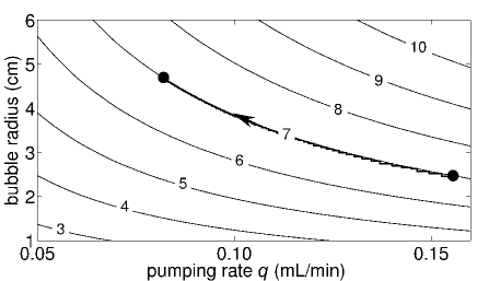
Figure 2: In order to grow an approximately $n$-fold symmetric bubble, the pumping rate is adjusted to follow (17), as illustrated here by curves for different $n$. The 7-fold bubble in Fig. 1(b) was grown in this way, as indicated by the bold line. We measure the area of a growing bubble in real time from the video images, and compute from that area a radius for a circle with that area. Then, given a target $n$-fold symmetry, the pumping rate is adjusted (in small steps) to stay on the desired $n$-fold curve of the graph. (These curves apply to a cell with gap thickness of 125 $\mu$m.)

After obtaining a nearly circular bubble, a multi-fingered bubble can be obtained by pumping oil out of the buffer. Usually fluid is removed at a fixed rate, as in our laboratory’s previous viscous fingering experiments Ristroph et al. (2006); Praud and Swinney (2005). However, with a fixed pumping rate, the $n$-fold mode that is the fastest growing changes with time, and the resultant bubble has many azimuthal modes with a substantial amplitude [e.g. Fig. 1(d)].

Our procedure for obtaining the harmonic moments and deducing the surface tension is applicable for bubbles grown with any pumping rate, $q(t)=bQ(t)$. However, results for the harmonic moments are more robust if a bubble retains an approximate $n$-fold symmetry as it grows. To achieve this, the pumping rate must decrease in a way that maintains an approximate $n$-fold symmetry. A linear stability analysis by Bataille Bataille (1968); Paterson (1981) provides an expression for the pumping rate needed to maintain the same $n$-fold perturbation of a circle as the fastest growing Bataille (1968); Paterson (1981) mode,

$$Q_{n}=\frac{{\pi}\sigma b^{2}}{6\mu R}(3n^{2}-1)$$ (17)

where $R$ is the radius of the bubble. The bubble radius $R$ given by the Bataille formula is plotted as a function of the volumetric pumping rate $q=bQ$ for different $n$-fold modes in Fig. 2. Conventional pumping with constant $Q$ would appear as a vertical trajectory in Fig. 2. For future experiments one should consider using Park-Homsy pressure jump, $p=-\sigma\kappa\pi/4$, instead of using Bataille’s assumption that $p=-\sigma\kappa$.

The particular multi-fingered pattern that develops depends not only on pumping rate but also on initial perturbations and non-uniformities of the glass plates. In the early stages of the pattern growth, when a bubble begins to deviate from a circle, small unavoidable departures from the circular shape have a greater influence on the development of the interface than the accuracy of pumping or non-uniformities of the glass plates. In practice, we found the smallest $m$ achievable was 5; for smaller target $m$ the growth was too slow to overcome initial perturbations on the bubble’s surface before the bubble reached the edge of the cell. We found that although the application of the Bataille formula for small perturbations of a circular bubble is not justifiable for bubbles that have grown large fingers, in practice the Bataille’s expression remains helpful in maintaining a symmetrical target pattern.

The present work concerns bubbles that are growing throughout an experiment. If the pumping were stopped, the surface tension would begin to smooth the interfacial regions of high curvature, and an interface could even reverse direction, absorbing the wetting film it left behind.

In most viscous fingering experiments where oil is withdrawn at a constant rate, the process has a natural separation of time scales: $t_{Q}=A/Q$, determined by pumping rate, is usually much less than the “capillary” time, $t_{\sigma}=48\mu R^{3}/(\sigma b^{2}n(n+1))$ (for not very high $n$), which corresponds to smoothing of a pattern by surface tension. The difference between time scales ($t_{\sigma}>>t_{Q}$) makes possible the rich interfacial patterns. However, in our case there is only a single time scale because the pumping $Q$ is adjusted continuously to maintain approximate $n$-fold symmetry. Equating the scales $t_{Q}\thicksim t_{\sigma}$, one recovers (within a multiplicative factor that depends on $n$) the Bataille formula. Note that for constant pumping the radius of a bubble is given by $R\thicksim\sqrt{t}$, while in our case $R\thicksim\sqrt[3]{t}$ (because $Q\thicksim 1/R$ and $R^{2}\thicksim Qt$).

IV.3 Image analysis

The oil/air interface in each image was first obtained by subtracting the background image, thresholding, and using an edge detection algorithm. This located the interface to within a pixel. The resolution of the interface was typically 50 pixels/cm, so that one pixel’s length was about 0.2 mm.

The position of each point on an interface was then obtained with sub-pixel accuracy by interpolating the location along a line perpendicular to the rough interface that was half of the intensity difference between the inside of the bubble (more intense) and the outside of the bubble (less intense). The algorithm typically found a position of half-intensity to 0.1 pixel (about 20 $\mu$m, which is small compared to the 125 $\mu$m or 384 $\mu$m plate separation). This procedure yielded a sufficiently smooth interface so that smoothing was not needed.

IV.4 Determing surface tension

Equation (16) is used to compute the surface tension. The time $t_{1}$ is chosen to be when the amplitude $a_{n}$ [given by (15)] of the perturbation from a circle exceeds 3 pixels. The time $t_{2}$ is chosen so that for slowly growing patterns about 10 images (60 s at 1 frame every 6 s) are collected in $t_{2}-t_{1}$; for rapidly growing patterns about 20 images (10 s at 2 frame/s) are obtained.

The velocity $V$ was calculated by projecting the local normal to the next later good interface. The use of splines allowed for the intersection to occur between interface points, so that the velocity could be computed more precisely. Sums of points of the interface were used as approximations of the contour integrals. The wetting correction (the second integral) contains the capillary number, $Ca=\mu V/\sigma$, which in our experiments was in the range $9\times 10^{-5}<\frac{\mu V}{\sigma}<2\times 10^{-2}.$ This range of $Ca$ is slightly larger than the range that Tabeling and Lichaber observed the 2/3 power law relation of the film thickness [cf. (13)] Tabeling and Libchaber (1986).

V RESULTS

V.1 Harmonic moments

We have calculated the harmonic moments $M_{k}(t)$ by evaluating the integrals in (16) for 16 bubbles grown in a cell with a 125 $\mu$m gap and for 10 bubbles grown in a Hele-Shaw cell with a 384 $\mu$m gap. For each bubble the values of $M_{k}(t)$ were computed for 50-500 data points spaced at time intervals 0.5-6 s.

We emphasize that our method for determining harmonic moments works well for asymmetric as well as symmetric bubbles. We chose to attempt to develop symmetric bubbles as they grew in order to track accurately the time evolution of particular moments $M_{k}$. Hence for each bubble the pumping rate was adjusted in real time according to (17), as described in Section V.B (cf. Fig. 2). Most of the bubbles evolved toward a targeted $n$-fold symmetry, which ranged from 5-fold (low pumping rate) to 14-fold (high pumping rate). However, some bubbles had an initial shape that was too irregular to evolve into an approximately $n$-fold bubble during the course of the growth; Fig. 4 is an example of such a bubble.

Our main result is that all observed moments $M_{k}(t)$ (except $M_{0}$) decay in time, as Fig. 3 illustrates. The next subsection presents results confirming that $dM_{k}/dt$ is proportional to the surface tension $\sigma$ (neglecting wetting correction) [cf. (14)], in accord with Richardson’s result that all moments are conserved in the zero surface tension case.

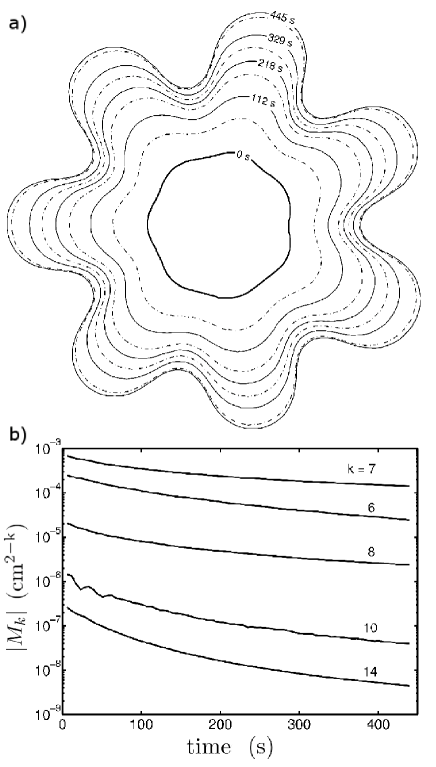
Figure 3: (a) An air bubble growing in oil in the Hele-Shaw cell (plate separation, 125 $\mu$m). Adjacent interfaces are separated by 56 s, and the maximum span of the bubble is 8 cm. The time-dependent pumping rate selects the 7-fold symmetry (cf. Fig. 2). (b) Amplitudes of moments 6, 7, 8, 10 and 14, computed using (6); note that different moments have different units. All moments decay in time, in contrast to the zero surface tension case where the moments are constant.

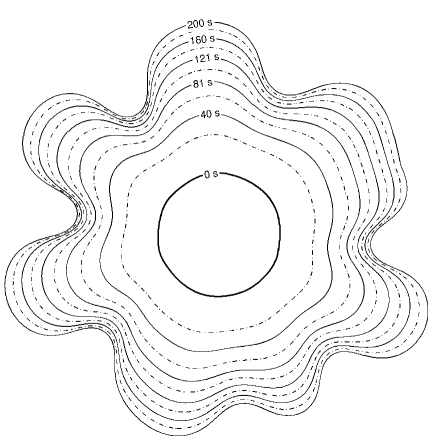
Figure 4: An air bubble growing without a clean $n$-fold symmetry. Adjacent interfaces are separated by 20 s.

V.2 Test of theory and determination of the surface tension

In the theoretical expression for $M_{k}(t_{2})-M_{k}(t_{1})$, equation (16), all quantities can either be determined from our measurements or from independent measurements. Hence the theory can be directly tested with no adjustable parameters.

We chose to present the test of theory as the ratio of the surface tension deduced from (16), which we call $\sigma_{measured}$, to the reference value of surface tension measured by the Wilhemy Plate method, $\sigma_{reference}$. Thus surface tension is treated as an unknown whose value can be deduced from (16), where the integrals and velocity $V$ are determined from analyses of the bubble patterns, while the viscosity $\mu$ and gap $b$ are measured independently.

An example of the results deduced for the surface tension ratio is shown in Fig. 5, which was computed for the non-symmetric bubble pattern in Fig. 4. For this bubble, the surface tension deduced without a wetting correction is 30% larger than the reference value at short times, where the front velocity is large (see Fig. 4), while at long times the front velocity has become smaller and the difference between the ratios with and without the wetting correction is only a few percent. Further, both ratios are within a few percent of unity, so the value of surface tension deduced from theory is equal to the reference value within the experimental uncertainty.

A measure of the symmetry of a bubble is given by the spectrum of the harmonic moments, i.e. a plot of the normalized moment amplitude, as shown in Fig. 6 for the symmetric bubble in Fig. 3 and for the non-symmetric bubble in Fig. 4. The approximately 7-fold bubble in Fig. 3 has a spectrum with significant components at 7, 14, and 21 [Fig. 6(a)], while the the non-symmetric bubble in Fig. 4 has a spectrum with a larger number of significant components, including those at 5, 6, 7, 8 [Fig. 6(b)].

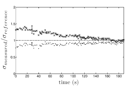
Figure 5: The ratio of the surface tension value deduced from theory for the data in Fig. 4 to the value independently measured by a traditional method (see text). The upper points ($\times$) are without a wetting correction, and the lower points ($\bullet$) are with the wetting correction in (16) [the term with the factor 3.8]. The error bars show the standard deviation for each group of points. The value of $t_{2}-t_{1}$ in (16) was 10 s. The horizontal axis corresponds to $t_{1}$.

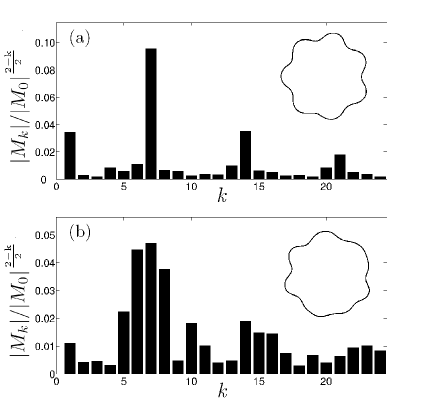
Figure 6: Spectra of the nondimensional moment amplitudes $|M_{k}|/|M_{0}|^{\frac{2-k}{2}}$ [equation (15)] for two bubbles: (a) A bubble with approximately 7-fold symmetry [Fig. 3(a)], where the main moments are 7, 14, and 21. The moments were calculated at the 112th second of the experiment. (b) A bubble without $n$-fold symmetry (Fig. 4), where there is a broad spectrum with no dominant moment. The moments were calculated at the 64th second of the experiment.

The mean value for the surface tension $\sigma_{measured}$ was deduced from (16), including the wetting correction, for each of the 26 bubbles studied, where each bubble was evaluated at 50-500 times during the course of its growth; this involved the numerical evaluation of the integrals in (16) for more than 6000 data sets. The result is $\sigma_{measured}$ = 18$\pm$4 mN/m, where the uncertainty includes both the statistical uncertainty and the estimated systematic uncertainty (see next paragraph). The result for $\sigma_{measured}$ agrees within the experimental uncertainty with $\sigma_{reference}=21.1\pm 0.1$ mN/m, determined by the Wilhelmy Plate method. Thus the theory is quantitatively confirmed within the experimental uncertainty. [If the wetting correction in (16) is neglected, the result for the surface tension is $23\pm 6$ mN/m.]

The uncertainty in our result for $\sigma_{measured}$ unfortunately arises in part from a possible systematic error of 9%. The uncertainty in gap thickness (about 4%) contributes significantly to the overall uncertainty. Also, an intermittent problem in camera synchronization could have introduced timing errors in some of the data. Other possible sources of error include the discretization of the integrals and the approximations introduced by the theoretical analysis. The range of applicability of the 2/3 scaling for the film thickness is smaller than the range of $Ca$ produced in our experiments. Another intriguing possible source of error is the 3.8 factor in the wetting correction Park and Homsy (1984), which has its origin in a numerical integration done in the 1974 PhD Dissertation by Ruschak Ruschak (1974). If the numerical factor of 3.8 were changed to 1.5, then the mean of the distribution in Fig. 7 would correspond to unity. Note that the wetting correction becomes small at long times because the growth velocity $V$ becomes small if the bubbles are grown according to (17).

The statistics of the results are presented in Fig. 7 as histograms of the ratio $\sigma_{measured}/\sigma_{reference}$, calculated both with and without the wetting correction. The distribution including the wetting correction is narrower because the uncorrected data depend on the pattern growth velocity. The mean value of the ratio with wetting correction is 0.84$\pm$0.09 (standard deviation, statistical uncertainty only); the mean value without wetting correction is 1.10$\pm$0.1(standard deviation).

Future experiments can straightforwardly reduce the systematic uncertainty by an order of magnitude to a level approaching 1%. Such experiments should focus on low order moments at intermediate times, to minimize the correction due to wetting and prevent backward motion of the interface.

Bubbles in our experiments were all studied for pumping rates $Q>0$. Alternatively, one could stop the growth (set $Q$=0) and observe the relaxation of a bubble. We conducted a few experiments in this way and found that the extracted surface tension values were typically 15-25% lower than those for growing bubbles. However, for relaxing bubbles the correction for the oil wetting film, which is re-absorbed as the interface retreats, is not known.

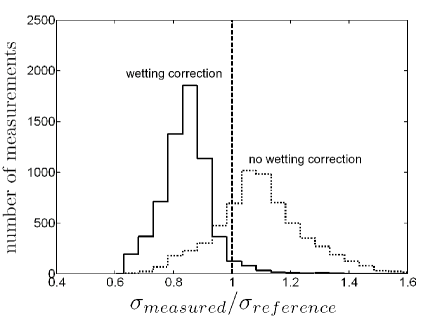
Figure 7: The distribution of the ratios of surface tension deduced from theory, $\sigma_{measured}$, to $\sigma_{reference}$, determined by the Wilhelmy Plate method. The solid line represents computations that include the wetting term, while the dotted line neglects the wetting correction. The bin size is 0.05. A few outlying points are outside of the abscissa’s range.

VI DISCUSSION

VI.1 Harmonic moments

We have presented the first demonstration that robust harmonic moments $M_{k}(t)$ can be deduced from laboratory experiments. The $M_{k}(t)$ evolve in time because of nonzero surface tension [Fig. 3(b)]; otherwise all moments except the area $M_{0}$ would be conserved. The harmonic moments are purely geometric quantities [cf. (6)] and do not involve approximations, fluid properties, or experimental parameters, such as the wetting correction, viscosity, or the gap thickness.

Further, we have obtained an equation for the dynamics of the harmonic moments, equation (16), which involves quantities that can all be directly determined by experiment, thus providing a quantitative test of the theory of harmonic moments. The result from measurements on 26 bubbles for two different Hele-Shaw cell gap thicknesses is that theory and experiment agree within the experimental uncertainty (about 20%). This agreement was obtained both on nonsymmetric bubbles and on bubbles with approximate $n$-fold symmetries varying from 5 to 14. This agreement is robust and, within our experiments, does not depend on how far a bubble has deviated from a circle. Further, we have indicated how it should be straightforward to reduce the experimental uncertainty by an order of magnitude, to test the theory at about a 1% level.

For convenience we have used an expression obtained by Bataille (17) to adjust the pumping rate $Q(t)$ to grow bubbles that are approximately $n$-fold symmetric. We find that if an $n$-fold bubble is grown initially from a slightly perturbed circle, the $n$-fold symmetry is retained even for large amplitude fingers, far beyond range of applicability of (17), which was obtained from a linear stability analysis.

VI.2 Implications

Harmonic moments $M_{k}$ form a complete basis for any complicated time domain $D$, provided that $D$ is analytic and singly connected. These moments are exceptionally useful for Laplacian growth phenomena such as viscous fingering because all other known representations involve coefficients that change quickly because of instability, thus creating analytic and computational difficulties. In contrast, harmonic moments are free of these problems, no matter how much the domain $D$ deviates from a circle. Loosely speaking, for harmonic moments the whole instability is simply concentrated in the lowest one, $M_{0}$ (the area of $D$).

From a fundamental perspective, the moments $M_{k}$ for Laplacian growth are exactly the basis that linearizes and “solves” the zero surface tension problem, generating a multitude of exact solutions (summarized in Mineev-Weinstein et al. (2008); see also references therein), which are impossible to obtain in any other basis. In this sense the harmonic moments constitute the most natural basis for Laplacian growth. Our experiments confirm that for nonzero surface tension, the derivative of the moments $dM_{k}/dt$ is simply proportional to $\sigma$ (neglecting the wetting correction), so that the zero surface tension limit is smoothly approached. This indicates that the fundamental theoretical results mentioned above, which have been obtained for Laplacian growth theory for the case of zero surface tension, are relevant to real physical systems.

In conclusion, the implications of the demonstration of the harmonic moments description of viscous fingering extends into various branches of mathematical physics (cf. Section II) because of the deep connection between Laplacian growth and other problems.

VII ACKNOWLEDGMENTS

We thank Olivier Praud for developing the method for maintaining an approximate $n$-fold symmetry of a bubble (Section IV.B), and we thank Dmitry Leshchiner for helpful discussions. Acknowledgment is made to the Donors of the American Chemical Society Petroleum Research Fund for support of this research. This work was also supported in part by the LDRD program 20070083ER at Los Alamos National Laboratory.

References

- Cross and Hohenberg (1993) M. C. Cross and P. C. Hohenberg, Rev. Mod. Phys. 65, 851 (1993).
- Gollub and Langer (1999) J. P. Gollub and J. S. Langer, Rev. Mod. Phys. 71, S396 (1999).
- Pelcé (1988) P. Pelcé, ed., Dynamics of Curved Fronts (Academic, Boston, 1988).
- Saffman and Taylor (1958) P. G. Saffman and G. Taylor, Proc. R. Soc. A 245, 312 (1958).
- Langer (1980) J. S. Langer, Rev. Mod. Phys 52, 1 (1980).
- Ben-Jacob (1997) E. Ben-Jacob, Contemporary Physics 38, 205 (1997).
- Hele-Shaw (1898) H. S. Hele-Shaw, Nature 58, 34 (1898).
- Lamb (1945) H. Lamb, Hydrodynamics (Dover, New York, 1945).
- Gillow and Howison (1998) K. A. Gillow and S. D. Howison (1998), URL http://www.maths.ox.ac.uk/~howison/Hele-Shaw/.
- Ristroph et al. (2006) L. Ristroph, M. Thrasher, M. B. Mineev-Weinstein, and H. L. Swinney, Phys. Rev. E 74, 015201(R) (2006).
- Segur et al. (1991) H. Segur, S. Tanveer, and H. Levine, eds., Asymptotics Beyond All Orders (Plenum, New York, 1991).
- Mineev-Weinstein et al. (2000) M. Mineev-Weinstein, P. B. Wiegmann, and A. Zabrodin, Phys. Rev. Lett. 84, 5106 (2000).
- Krichever et al. (2004) I. Krichever, M. Mineev-Weinstein, P. Wiegmann, and A. Zabrodin, Physica D 198, 1 (2004).
- Mineev-Weinstein et al. (2008) M. Mineev-Weinstein, M. Putinar, and R. Teodorescu, Journal of Physics A, Math. Theor. 41, 263001 (2008).
- Ciliberto and Gollub (1984) S. Ciliberto and J. P. Gollub, Phys. Rev. Lett. 52, 922 (1984).
- Sawada et al. (1986) Y. Sawada, A. Dougherty, and J. P. Gollub, Phys. Rev. Lett. 56, 1260 (1986).
- Witten and Sander (1981) T. A. Witten and L. M. Sander, Phys. Rev. Lett. 47, 1400 (1981).
- Zubarev (2002) N. M. Zubarev, JETP Lett. 94, 534 (2002).
- Praud and Swinney (2005) O. Praud and H. L. Swinney, Phys. Rev. E 72, 011406 (2005).
- Kessler et al. (1988) D. A. Kessler, J. Koplik, and H. Levine, Adv. Phys. 37, 255 (1988).
- Langer and Muller-Krumbhaar (1978) J. S. Langer and H. Muller-Krumbhaar, Acta Metallurgica 26, 1681 (1978).
- Halsey (2000) T. C. Halsey, Physics Today 53, 36 (2000).
- Richardson (1972) S. Richardson, J. of Fluid Mech. 56, 609 (1972).
- Mineev (1990) M. B. Mineev, Physica D 43, 288 (1990).
- Novikoff (1938) P. S. Novikoff, Dokl. Akad. Nauk SSSR [Sov. Phys. Dokl.] 18, 165 (1938).
- Etingof and Varchenko (1992) P. I. Etingof and A. N. Varchenko, vol. 3 (AMS, Providence, RI, 1992).
- Jackson (1999) J. D. Jackson, Classical Electrodynamics (Wiley, New York, 1999), 3rd ed.
- Landau (1987) H. J. Landau, Moments in Mathematics (AMS, Providence, RI, 1987).
- Gustafsson and Putinar (2007) B. Gustafsson and M. Putinar, Physica D 235, 90 (2007).
- Aharonov and Shapiro (1976) D. Aharonov and H. S. Shapiro, J. Analyse Math. 30, 39 (1976).
- Sakai (1982) M. Sakai, Quadrature Domains, vol. 934 of Lecture Notes in Math. (Springer-Verlag, Berlin, 1982).
- Golub et al. (1999) G. H. Golub, P. Milanfar, and J. Varah, SIAM J Sci. Comput. 21, 1222 (1999).
- Gustafsson et al. (2000) B. Gustafsson, C. He, P. Milanfar, and M. Putinar, Inverse Problems (Institute of Physics, Bristol, 2000), vol. 16, p. 1053.
- Park and Homsy (1984) C.-W. Park and G. M. Homsy, J. Fluid Mech. 139, 291 (1984).
- Tabeling and Libchaber (1986) P. Tabeling and A. Libchaber, Phys. Rev. A 33, 794 (1986).
- Bataille (1968) J. Bataille, Rev. Inst. Fr. Pet. Ann. Combust. Liq. 23, 1349 (1968).
- Paterson (1981) L. Paterson, J. Fluid Mech. 113, 513 (1981).
- Ruschak (1974) K. J. Ruschak, Ph.D. thesis (University of Minnesota, 1974).