Condenser physics applied to Markov chains
– A brief introduction to potential theory –

These notes are based on a collective discussion that started with Alessandra Bianchi in December 2007 at the WIAS in Berlin and went on during the next two months in Rome 2 and 3 with Tony Iovanella, Francesco Manzo, Francesca Nardi, Koli Ndreca, Enzo Olivieri, Betta and Benedetto Scoppola, Alessio Troiani and Massimiliano Viale. Since all of us were working on arguments more or less strongly related to metastability, we all felt the need to understand in some or more depth the links between potential theory and Markov processes on which are based the tools coming from the former that Bovier, Eckoff, Gayrard and Klein introduced in the study of metastability [22] and were successfully applied in [24], [25], [28], [34], [35] among other papers. Many mathematicians and physicists are certainly well aware of these links but, at various degrees, it was not our case and we thought that a good understanding of this connection was an essential support to intuition and a precious guide in the use of these tools. As J.L. Doob once put it: “To learn potential theory from probability is like learning algebraic geometry without geometry.” [4] This explains why before going to the specific application to metastability I will essentially focus on potential theory and Markov processes for themselves.

Still because concerned by the leading ideas founding the connections between potential theory and Markov processes I will write complete proofs only in the simplest context that allows for avoiding any technicality and makes more transparent these connections: that of Markov chains on a finite state space ${\cal X}$ (and this does not exclude working in the regime where the cardinality $|{\cal X}|$ goes to infinity). We will not however restrict our analysis to this simpler setting. Potential theory begun indeed in a quite different form during the last three decades of the XVIII century with the works of Lagrange and Laplace that described the gravitational field as deriving from a potential $V$ solution of the Laplace equation

$$\Delta V\equiv 0$$ (0.1)

and blossomed in the first half of the XIX century as the cornerstone of electrostatic, in particular with Gauss and Green’s works. This development was so important that the study of harmonic functions, that is of the solutions of the Laplace equation, used to be one of the main pillar of the accademic formation of any physicist or mathematician at the end of the century.

The study of Markov processes started with Markov at the beginning of the next century but, as far as I know, it was not before the last years of the second world war that the links with potential theory begun to be drawn by Kakutani [2]. It took then almost 40 years to make this connection fully developed. In 1984 Doob published his treaty Classical Potential Theory and its Probabilistic Counterpart [4] and in the same year Doyle and Snell wrote their beautiful article [6] that embraced in a same light the mathematics of random walks and the physics of electrical networks. Since then people did not stop harvesting the fruits of such a fertile union. See for example: [3], [15], [26], [30], [36], [37].

A final motivation for writing these notes is that we could not find (although it probably exists) a single synthetic text that linked together the electrostatic of original potential theory, the physics of electric networks and the probabilistic meaning of the objects they contemplate. But I want to point out a few classics that I found particularly useful to write these notes, even though some are not mainly or directly linked to the subject: together with Doyle and Snell’s article [6] there were Norris’ book [20], Lyons and Peres’ continuously updated online book [17], Karatzas and Shreve’s book [10], Sinclair’s paper [14], and Lawler’s book [11]. I want also to thank here Pietro Caputo and Alessandra Faggionato for the many discussions we had that considerably enriched these notes.

1 Laplace equation

1.1 Harmonic functions

In this section and the next one ${\cal U}$ will denote an open subset of the $d$-dimensional vector space ${\mathbb{R}}^{d}$. For $x$ in ${\mathbb{R}}^{d}$ we will write $x_{1}$, $x_{2}$, …, $x_{d}$ for its coordinates and we will use the notation $B_{2}(x,r)$ for the open Euclidean ball of centre $x$ and radius $r>0$.

Definition 1.1.1

For $f\in{\cal C}^{2}({\cal U},{\mathbb{R}})$ we define the Laplacian of $f$ as

$$\Delta f:x\in{\cal U}\mapsto\Delta_{x}f:=\sum_{k=1}^{d}\frac{\partial^{2}f}{\partial x_{k}^{2}}(x)\in{\mathbb{R}}$$ (1.1)

and we say that $f$ is harmonic on ${\cal U}$ when it satisfies the Laplace equation on ${\cal U}$

$$\forall x\in{\cal U},\>\Delta_{x}f=0$$ (1.2)

Examples: With

$$r:(x_{1},\dots,x_{d})\in{\mathbb{R}}^{d}\mapsto\sqrt{x_{1}^{2}+\dots+x_{d}^{2}}$$ (1.3)

a harmonic function on ${\mathbb{R}}^{d}\setminus\{0\}$ is $r$ if $d=1$, $\ln r$ if $d=2$ and $r^{2-d}$ if $d\geq 3$.

The previous definition is a good one in the measure in which it frames harmonic functions inside differential calculus with all the tools it provides. But this definition looks to harmonic functions from an essentially local point of view. It has to be reformulated to make transparent larger scale properties of harmonic functions.

For $f\in{\cal C}^{1}({\cal U},{\mathbb{R}})$ we will denote by $\nabla f$ or $\vec{\nabla f}$ or ${\rm grad}f$ its gradient

$${\rm grad}f:x\in{\cal U}\mapsto\nabla_{x}f:=\left(\frac{\partial f}{\partial x_{k}}(x)\right)_{1\leq k\leq d}\in{\mathbb{R}}^{d}$$ (1.4)

For $\phi\in{\cal C}^{1}({\cal U},{\mathbb{R}}^{d})$ we will denote by ${\rm div}\phi$ or $\nabla\phi$ its divergence

$$\nabla\phi:x\in{\cal U}\mapsto{\rm div}_{x}\phi:=\sum_{k=1}^{d}\frac{\partial\phi_{k}}{\partial x_{k}}(x)\in{\mathbb{R}}$$ (1.5)

Hence, saying that $f$ is harmonic on ${\cal U}$ is saying that

$${\rm div}({\rm grad}f)\equiv 0$$ (1.6)

or, equivalently, that $\nabla f$ is a null divergence field. Now Stokes’ lemma makes possible to switch from the local point of view to a larger scale one.

Lemma [Stokes] Let $\vec{\phi}\in{\cal C}^{1}({\cal U},{\mathbb{R}}^{d})$ and ${\cal V}$ be an open subset of ${\cal U}$ with a compact closure $\overline{{\cal V}}\subset{\cal U}$ and such that $\partial{\cal V}$ is a (smooth) submanifold of ${\mathbb{R}}^{d}$. Then

$$\int_{\partial{\cal V}}\vec{\phi}.\vec{dS}:=\int_{\partial{\cal V}}\vec{\phi}.\vec{n}\,d\sigma=\int_{\cal V}{\rm div}\vec{\phi}\,d\lambda$$ (1.7)

where $\vec{n}$ is the unitary vector that is orthogonal to $\partial{\cal V}$ and oriented from ${\cal V}$ towards ${\cal U}\setminus{\cal V}$, while $\sigma$ and $\lambda$ stand for the surface and volume Lebesgue measure respectively.

Stokes’ lemma is a straightforward identity in its discrete version (see Section 2.2) and we just assume it in its continuous one. It implies that for a harmonic function $f$ on ${\cal U}$ and such a closed oriented smooth surface $\partial{\cal V}\subset{\cal U}$ the flux of the vector field $\nabla f$ through $\partial{\cal V}$ is zero. And as a first consequence we get:

Proposition 1.1.2 (Mean-value property)

If $f$ is harmonic on ${\cal U}$ then $f$ satisfies the mean-value property (m.v.p.), that is:

$$\forall r>0,\,\forall x\in{\cal U},\,\overline{B_{2}(x,r)}\subset{\cal U}\Rightarrow f(x)=\int_{\partial B_{2}(x,r)}f\frac{d\sigma}{|\partial B_{2}(x,r))|}$$ (1.8)

where $|\partial B_{2}(x,r)|$ denotes the surface area of $\partial B_{2}(x,r)$, in such a way that the integral computes the mean value of $f$ on $\partial B_{2}(x,r)$.

Proof: We pick $x$ in ${\cal U}$ and define, for all $r>0$ such that $\overline{B_{2}(x,r)}\subset{\cal U}$,

$$g(r):=\int_{\partial B_{2}(x,r)}f\,\frac{d\sigma}{|\partial B_{2}(x,r)|}\\ =\int_{\partial B_{2}(0,1)}f(x+ru)d\sigma_{1}(u)$$ (1.9)

with $\sigma_{1}$ the uniform probability measure on $\partial B_{2}(0,1)$. By continuity of $f$,

$$\lim_{r\rightarrow 0}g(r)=f(x)$$ (1.10)

Then, we just need to show that $g$ is constant, i.e., has a null derivative. Fix $r$ small enough to have $g(r)$ that is well defined. For all small enough real $h$ and $u\in\partial B_{2}(0,1)$, the Taylor formula gives

$$f(x+(r+h)u)=f(x+ru)+h\frac{\partial f}{\partial u}(x+ru)+\int_{0}^{h}(h-t)\frac{\partial^{2}f}{\partial u^{2}}(x+(r+t)h)dt$$ (1.11)

so that, integrating over $\partial B_{2}(0,1)$ and using $f\in{\cal C}^{2}({\cal U})$ to control the second derivative in the integral,

$$g(r+h)=g(r)+\frac{h}{|\partial B_{2}(x,r)|}\int_{\partial B_{2}(x,r)}\vec{\nabla f}.\vec{dS}+o(h)$$ (1.12)

By Stokes’ lemma the integral in this sum is zero and we conclude $g^{\prime}(r)=0$.     $\Box$

Actually the mean-value property characterizes harmonic functions and gives additional information on their regularity:

Proposition 1.1.3

If $f\in{\cal C}({\cal U})$ has the m.v.p. then

• $f\in{\cal C}^{\infty}({\cal U})$;

• f is harmonic on ${\cal U}$.

Proof: The proof of i) is based on a simple convolution argument that can be find in [10] page 242. Now, if $f$ is not harmonic, then we can find $x\in{\cal U}$ and $r_{0}>0$ such that ${\rm div}\nabla f$ is strictly positive (or strictly negative) on $B_{2}(x,r_{0})\subset{\cal U}$. Then the derivation of the previous proof shows, with Stokes’ lemma, that the function $g$ defined in (1.9) is strictly monotone in the neighbourhood of $0$. And this contradicts the m.v.p.     $\Box$

The m.v.p. leads also to the following

Proposition 1.1.4 (Maximum principle)

If $f$ is harmonic on ${\cal U}$ then, for all compact sets $K\subset\overline{{\cal U}}$ such that $f$ can be extended by continuity on $K$, $f|_{K}$ reaches its maximum (and its minimum) on $\partial K$.

Proof: Set $M:=\max f(K)$. If $\partial K$ and $f|_{K}^{-1}\{M\}$ were disjoint sets then we could find $x$ in $\partial f|_{K}^{-1}\{M\}$ and $r>0$ such that $\overline{B_{2}(x,r)}\subset K\cap{\cal U}$. The m.v.p would give

$$M=f(x)=\int_{\partial B_{2}(x,r)}f\frac{d\sigma}{|\partial B_{2}(x,r)|}$$ (1.13)

while the continuity of $f$ in some $y\in(\partial B_{2}(x,r))\setminus f|_{K}^{-1}\{M\}$ would give

$$\int_{\partial B_{2}(x,r)}f\frac{d\sigma}{|\partial B_{2}(x,r)|}<M$$ (1.14)

what would be a contradiction.     $\Box$

The maximum principle is sometimes reported in the electrostatic context as: “The potential has no local extremum where there is no charge.” Indeed Gauss’ law in Maxwell’s equations reads

$${\rm div}\vec{E}=\frac{\rho}{\epsilon_{0}}$$ (1.15)

where $\rho$ stands for the charge density, $\epsilon_{0}$ is the electric constant and $\vec{E}$ is the electric field that derives from a potential $V$, that is

$$\vec{E}=-\nabla V$$ (1.16)

A “local extremum where there is no charge” would be an isolated local extremum somewhere in the interior ${\cal U}$ of $\rho^{-1}\{0\}$, where the potential $V$ is harmonic by (1.15) and (1.16). And that would be in contradiction with the maximum principle.

The maximum principle opens the door to uniqueness properties of the solution of the Dirichlet problem.

Definition 1.1.5 (Dirichlet problem)

Given $g\in{\cal C}(\partial{\cal U},{\mathbb{R}})$ we say that $f$ is a solution of the Dirichlet problem on ${\cal U}$ with boundary condition $g$ if $f$ in ${\cal C}^{2}({\cal U})$ and ${\cal C}(\overline{{\cal U}})$ satisfies the Laplace equation on ${\cal U}$ and coincides with $g$ on $\partial{\cal U}$.

Examples: i) Consider a compact thermal conductor $K$, fix to $g(x)$ the temperature in each point $x$ of $\partial K$ and assume that $g$ is continuous on $\partial K$. If the temperature reaches an equilibrium $f(x)$ in each point of the interior ${\cal U}$ of the conductor, then $f$ will be solution of the Dirichlet problem on ${\cal U}$ with boundary condition $g$. Let us assume the existence of such an equilibrium temperature. The maximum principle gives us the uniqueness of the equilibrium temperature. Indeed if $f_{1}$ and $f_{2}$ are both solutions, then $f_{1}-f_{2}$ is solution of the Dirichlet problem with zero boundary condition. Then, on ${\cal U}$, $f_{1}-f_{2}$ cannot take values larger than the maximum value on the border, that is 0, or smaller that the minimum value on the border, 0 once again: $f_{1}$ and $f_{2}$ coincide both on ${\cal U}$ and $\partial{\cal U}$.

ii) Consider a finite number of (disjoint) compact electric conductors $A_{1}$, …, $A_{n}$ and fix at values $V_{1}$, …, $V_{n}$ on these conductors the difference of potential with infinity. There cannot be any charge outside the conductors, so that, by (1.15), (1.16) and taking the convention that the potential is $0$ at infinity, a potential $V$ has to be solution of the Dirichlet problem on the complementary of $\cup_{n}A_{n}$ with boundary condition $V_{k}$ on $\partial A_{k}$ for $k$ in $\{1;\dots;n\}$ and with the additional condition

$$\lim_{x\rightarrow\infty}V(x)=0$$ (1.17)

Once again the maximum principle gives the uniqueness of the potential $V$ under an existence hypothesis.

Proving the existence of a solution of a Dirichlet problem turns out to be a rather difficult task when one stay inside the framework of plain functional analysis. It is time to turn to Markov processes.

1.2 Brownian motion

For simplicity we will now assume that ${\cal U}$ is a bounded open domain. For extensions and generalizations to unbounded domains of the results presented here we refer to [10] section 4.2. We denote by $P_{x}$ the law of a $d$-dimensional Brownian motion $W$ starting from $x\in{\mathbb{R}}^{d}$ and by $\tau_{A}$ the hitting time of any set $A$:

$$\tau_{A}=\inf\left\{t\geq 0:\>W(t)\in A\right\}$$ (1.18)

Katunani’s idea [2] was to present the candidate

$$h:x\in\overline{\cal U}\mapsto E_{x}\left[g\left(W(\tau_{\partial{\cal U}})\right)\right]$$ (1.19)

to solution of the Dirichlet problem on ${\cal U}$ with boundary condition $g$. Since $\overline{\cal U}$ is a compact set we have, for all $x$ in $\overline{\cal U}$,

$$P_{x}(\tau_{\partial{\cal U}}<+\infty)=1$$ (1.20)

so that $h$ is well defined. We clearly have $h|_{\partial{\cal U}}=g$ and $h$ has the m.v.p. Indeed, for any $x\in{\cal U}$ and $r>0$ such that $\overline{B_{2}(x,r)}\subset{\cal U}$, we have, by the strong Markov property at time $\tau_{\partial B_{2}(x,r)}$ and using radial symmetry:

$$h(x) = E_{x}\left[g\left(W(\tau_{\partial{\cal U}})\right)\right]$$ (1.21)

$$= E_{x}\left[E_{x}\left[g\left(W(\tau_{\partial{\cal U}})\right)\Big{|}W(\tau_{\partial B_{2}(x,r)})\right]\right]$$ (1.22)

$$= \int_{y\in\partial B_{2}(x,r)}E_{y}\left[g\left(W(\tau_{\partial{\cal U}})\right)\right]dP_{x}(W(\tau_{\partial B_{2}(x,r)})=y)$$ (1.23)

$$= \int_{\partial B_{2}(x,r)}h(y)\frac{d\sigma(y)}{|\partial B_{2}(x,r)|}$$ (1.24)

As a consequence $h$ is harmonic on ${\cal U}$ and the only point to check to get a solution of the Dirichlet problem is the continuity of $h$ on $\overline{\cal U}$. This question is intimately linked to the notion of regularity.

Definition 1.2.1

For any set $A$ we define

$$\tau^{+}_{A}:=\inf\left\{t>0:\>W(t)\in A\right\}$$ (1.25)

and we say that ${\cal U}$ has a regular border when

$$\forall a\in\partial{\cal U},\;P_{a}\left(\tau^{+}_{{\cal U}^{c}}=0\right)=1$$ (1.26)

Proposition 1.2.2

A bounded open domain ${\cal U}$ has a regular border if and only if, for all $g$ in ${\cal C}(\partial{\cal U})$ the function $h$ defined in (1.19) is continuous on $\overline{\cal U}$,i.e., is solution of the associated Dirichlet problem.

We refer to [10] for the proof (of a stronger result). We give now some examples.

In dimension two and for $b>a>0$ consider the Dirichlet problem on

$${\cal U}=B_{2}(0,b)\setminus\overline{B_{2}(0,a)}$$ (1.27)

with boundary conditions $1$ on $\partial B_{2}(0,a)$ and $0$ on $\partial B_{2}(0,b)$.

On the one hand, since $\ln r$ is harmonic, we have the solution

$$f=\frac{\ln b-\ln r}{\ln b-\ln a}$$ (1.28)

By the maximum principle $f$ is the unique solution ($\overline{\cal U}$ is a compact set).

On the other hand ${\cal U}$ has a regular border. Indeed a Brownian motion that starts from $x$ in $\partial{\cal U}$ crosses $\partial{\cal U}$ infinitely many times during any time interval $[0;t]$ with $t>0$. As a consequence the function $h$ defined in (1.19) is solution of the problem and coincides with $f$. That reads

$$\forall x\in{\mathbb{R}}^{2},\;a\leq r(x)\leq b\Rightarrow P_{x}\left(\tau_{\partial B_{2}(0,a)}<\tau_{\partial B_{2}(0,b)}\right)=\frac{\ln b-\ln r(x)}{\ln b-\ln a}$$ (1.29)

Consider now the Dirichlet problem on the punctured ball

$${\cal U}=B_{2}(0,b)\setminus\{0\}$$ (1.30)

This example will have some relevance later when dealing with metastability in large volume (Section 6.4). Sending $a$ to 0 in (1.29) we get

$$\forall x\in\overline{B_{2}(0,b)}\setminus\{0\},\;P_{x}\left(\tau_{\{0\}}<\tau_{\partial B_{2}(0,b)}\right)=0$$ (1.31)

This implies that the function $h$ defined in (1.19) is equal to ${\tt 1\tt l}_{\{0\}}$. It is not continuous and 0 is not regular, as it could directly be seen from (1.31). Such examples of domain with a non regular border can be built with a connected border in dimension $d\geq 3$.

In the last example our candidate to solution for our problem on the punctured ball lost the election. But could have we find another solution? The answer is no: using the uniqueness of an eventual solution $f$ and the radial symmetry of the problem we can show that $f$ would be a simple function of $r$, then solving the Laplace equation in polar coordinates we would get

$$f=\alpha+\beta\ln r$$ (1.32)

with $\alpha$ and $\beta$ constants, the continuity in 0 would imply $\beta=0$ and the boundary conditions could not be conciliated. More generally:

Proposition 1.2.3

If the Dirichlet problem on a bounded open domain ${\cal U}$ with boundary condition $g$ has a solution $f$, then $f$ coincides with $h$ defined in (1.19).

Proof: For all positive integer $n$ we define

$${\cal U}_{n}:=\left\{x\in{\cal U}:\>d_{2}(x,\partial{\cal U})>\frac{1}{n}\right\}$$ (1.33)

Note that ${\cal U}_{n}$ has a regular border since for all $a$ in $\partial{\cal U}_{n}$ $a$ is on the border of a ball (of radius 1/n) contained in ${\cal U}_{n}^{c}$. We also define

$$h_{n}(x):x\in\overline{\cal U}\mapsto E_{x}\left[f(W(\tau_{{\cal U}_{n}^{c}}))\right]$$ (1.34)

The functions $f$ and $h_{n}$ coincide on ${\cal U}_{n}^{c}$, and they coincide on ${\cal U}_{n}$ too: since ${\cal U}_{n}$ has a regular border, both are solution of the Dirichlet problem on ${\cal U}_{n}$ with boundary condition $f|_{\partial{\cal U}_{n}}$, since $\overline{{\cal U}_{n}}$ is a compact set, this solution is unique by the maximum principle. Now $f$ is bounded as continuous function on the compact set $\overline{\cal U}$, and by dominated convergence we get, for all $x$ in $\overline{\cal U}$,

$$f(x)=\lim_{n\rightarrow+\infty}h_{n}(x)=h(x)$$ (1.35)

$\Box$

The probabilistic approach to potential theory does not only solve some of the problems regarding the existence of a potential. It also laid the ground to receive deep insight from potential theory into Markov processes theory. For example formula (1.29) gives the recurrence of the two-dimensional Brownian motion: send $b$ to infinity to get

$$\forall x\not\in B_{2}(0,a),\;P_{x}(\tau_{\partial B_{2}(0,a)}<+\infty)=1$$ (1.36)

The same potential study in dimension $d\geq 3$ gives

$$\forall x\in{\mathbb{R}}^{d},\;a\leq r(x)\leq b\Rightarrow P_{x}\left(\tau_{\partial B_{2}(0,a)}<\tau_{\partial B_{2}(0,b)}\right)=\frac{r(x)^{2-d}-b^{2-d}}{a^{2-d}-b^{2-d}}$$ (1.37)

and the transience of the Brownian motion:

$$\forall x\not\in\overline{B_{2}(0,a)},\;P_{x}(\tau_{\partial B_{2}(0,a)}<+\infty)=\left(\frac{r}{a}\right)^{2-d}<1$$ (1.38)

We close this section with a last illustration of the evocative power of Kakutani’s solution. Consider a single electric compact conductor $K$ at potential 1 in ${\mathbb{R}}^{3}$. By the so-called “point-effect” the electric field will be stronger in the neighbourhood of the points $a$ of the convex parts of $K$ with strong curvature. Indeed

$$\vec{E}=-\nabla V$$ (1.39)

and Kakutani’s solution for the potential $V$ outside $K$ gives

$$V(x)=P_{x}\left(\tau_{K}<+\infty\right)$$ (1.40)

(take the increasing limit of the solution of the Dirichlet problem on $B_{2}(0,R)\setminus K$ with potential 0 on $\partial B_{2}(0,R)$ when $R$ goes to infinity.) Loosely speaking (we will give a stronger justification of the point-effect in Section (4.1)) the escape probability can decrease much faster in the neighbourhood of such points $a$. And this why lightning rods are rods: a stronger field in the neighbourhood of the rod makes easier to reach the disruptive field there before than somewhere else.

1.3 Discrete Laplacian and simple random walks

Going from ${\mathbb{R}}^{d}$ to ${\mathbb{Z}}^{d}$ we loose the differential tool: derivatives have to be replaced by their discrete version. Denoting by ${\cal E}$ the symmetric subset of ${\mathbb{Z}}^{d}\times{\mathbb{Z}}^{d}$ made of the nearest neighbour sites

$${\cal E}:=\left\{e=(e_{-},e_{+})\in({\mathbb{Z}}^{d})^{2}:\>d_{1}(e_{-},e_{+})=1\right\}$$ (1.41)

the gradient of a real valued function $f$ on ${\mathbb{Z}}^{d}$ becomes an antisymmetric real valued function on ${\cal E}$:

$$\nabla f:e\in{\cal E}\mapsto\nabla_{e}f:=f(e_{+})-f(e_{-})\in{\mathbb{R}}$$ (1.42)

and the divergence of such an antisymmetric function $\phi$ on ${\cal E}$ turns to be a real valued function on ${\mathbb{Z}}^{d}$:

$${\rm div}\phi:x\in{\mathbb{Z}}^{d}\mapsto{\rm div}_{x}\phi:=\sum_{\stackrel{{\scriptstyle\scriptstyle e\in{\cal E}}}{{\scriptstyle e_{-}=x}}}\phi(e)\in{\mathbb{R}}$$ (1.43)

The discrete Laplacian of $f$ is then defined by

$$\Delta f:x\in{\mathbb{Z}}^{d}\mapsto\Delta_{x}f:={\rm div}_{x}(\nabla f)=\sum_{\stackrel{{\scriptstyle\scriptstyle y\in{\mathbb{Z}}^{d}}}{{\scriptstyle d_{1}(x,y)=1}}}(f(y)-f(x))$$ (1.44)

Note that this is coherent with second order Taylor developments: for $f$ in ${\cal C}^{2}({\mathbb{R}}^{d})$ and a unitary vector $u$

$$\frac{\partial^{2}f}{\partial u^{2}}(x)=\lim_{\stackrel{{\scriptstyle\scriptstyle h\rightarrow 0}}{{\scriptstyle h\in{\mathbb{R}}}}}\frac{f(x+hu)+f(x-hu)-2f(x)}{h^{2}}$$ (1.45)

For ${\cal U}\subset{\mathbb{Z}}^{d}$ the border of ${\cal U}$ is

$$\partial{\cal U}:=\left\{e=(e_{-},e_{+})\in{\cal E}:\>e_{-}\in{\cal U},e_{+}\not\in{\cal U}\right\}$$ (1.46)

and its external border is

$$\partial_{+}{\cal U}:=\left\{e_{+}\in{\mathbb{Z}}^{d}:\>\exists e=(e_{-},e_{+})\in\partial{\cal U}\right\}$$ (1.47)

A function $f$ defined on ${\cal U}\cup\partial_{+}{\cal U}$ is harmonic on ${\cal U}$ if

$$\forall x\in{\cal U},\;\Delta_{x}f=0$$ (1.48)

Observe that (1.48) expresses a local mean-value property: it is equivalent to

$$\forall x\in{\cal U},\;\frac{1}{2d}\Delta_{x}f=\left(\frac{1}{2d}\sum_{\scriptstyle d_{1}(x,y)=1}f(y)\right)-f(x)=0$$ (1.49)

The set of harmonic functions on ${\mathbb{Z}}^{d}$ is the kernel of the generator of the (continuous time) simple random walk, $\frac{1}{2d}\Delta$, just like the set of harmonic functions on ${\mathbb{R}}^{d}$ was the kernel of the generator of Brownian motion, $\frac{1}{2}\Delta$.

Like in the continuous case the mean-value property of harmonic functions gives a maximum principle (for which the notion of compactness is replaced by that of finiteness), and this maximum principle can be used to show uniqueness properties for the solutions of Dirichlet problems. Given ${\cal U}\subset{\mathbb{Z}}^{d}$ and $g$ a real valued function on its external border, we say that $f$ is a solution of the Dirichlet problem on ${\cal U}$ with boundary condition $g$ if $f$ is harmonic on ${\cal U}$ and $f$ coincides with $g$ on $\partial_{+}{\cal U}$. Just like we used Brownian motion to prove the existence of a solution for some Dirichlet problem, we can do the same with simple random walks on ${\mathbb{Z}}^{d}$. For example:

Proposition 1.3.1

For any finite subset ${\cal U}$ of ${\mathbb{Z}}^{d}$ and any real valued function $g$ on $\partial_{+}{\cal U}$, there is a unique solution of the Dirichlet problem on ${\cal U}$ with boundary condition $g$. This solution is the function $h$ defined by

$$\forall x\in{\cal U}\cup\partial_{+}{\cal U},\;h(x):=E_{x}\Big{[}g\left(\zeta(\tau_{{\cal U}^{c}})\right)\Big{]}$$ (1.50)

where $E_{x}$ stands for the expectation under the law of a simple random walk $\zeta$ that start from $x$.

Proof: By the Markov property, $h$ satisfies the local mean-value property on ${\cal U}$. Since $h$ and $g$ coincide on $\partial_{+}{\cal U}$, $h$ is solution of the Dirichlet problem. It is the only one by application of the maximum principle.     $\Box$

2 Electrical networks

2.1 Random walks and generators

An electrical network is a connected undirected weighted graph with positive weights, with no more than one edge between any pair of vertices and with finite total weight on each vertex. More formally it is a pair $({\cal X},c)$ with ${\cal X}$ a countable set and $c$ a real valued non-negative symmetric function on ${\cal X}\times{\cal X}$ such that

$$\forall x\in{\cal X},\;\mu(x):=\sum_{y\in{\cal X}}c(x,y)<+\infty$$ (2.1)

and such that, for all distinct $x$ and $y$ in ${\cal X}$, there exist $x=z_{1}$, $z_{2}$, …, $z_{n}=y$ in ${\cal X}$ with

$$\forall k\in\{1;\dots;n-1\},\;c(z_{k},z_{k+1})>0$$ (2.2)

We call nodes the elements of ${\cal X}$, we say that two nodes $x$ and $y$ are connected when $c(x,y)>0$ and we call edges the elements of ${\cal E}$, defined as the set of ordered pairs of connected nodes:

$${\cal E}:=\left\{(x,y)\in{\cal X}\times{\cal X}:\>c(x,y)>0\right\}$$ (2.3)

Of course the edges in ${\cal E}$ do have a direction, but it is better to keep in mind the image of an undirected graph for which each pair of connected nodes can have two representatives in the symmetric subset ${\cal E}$ of ${\cal X}\times{\cal X}$. The conductance between two nodes $x$ and $y$ is $c(x,y)$ and the resistance between $x$ and $y$ is

$$r(x,y):=\frac{1}{c(x,y)}\in]0;+\infty]$$ (2.4)

Note that 0 and $+\infty$ are possible values for $c(x,y)$ and $r(x,y)$: when $(x,y)$ is not in ${\cal E}$.

We call potential any real valued function on ${\cal X}$. If we impose a potential $g(x)$ on each node $x$ outside a subset ${\cal U}$ of ${\cal X}$, an equilibrium potential $V$ associated with the constraint

$$\forall x\in{\cal U}^{c},\;V(x)=g(x)$$ (2.5)

has to satisfy Ohm’s and Kirchoff’s laws.

Ohm’s law: The current $i$ associated with $V$ is

$$i:(x,y)\in{\cal E}\mapsto i(x,y)=\frac{V(x)-V(y)}{r(x,y)}$$ (2.6)

Kirchoff’s law: For all $x$ in ${\cal U}$

$$\sum_{\stackrel{{\scriptstyle\scriptstyle y\in{\cal X}}}{{\scriptstyle(x,y)\in{\cal E}}}}i(x,y)=0$$ (2.7)

In other words

$$\forall x\in{\cal U},\;-{\cal L}_{x}V=0$$ (2.8)

with, for any potential $f$,

$${\cal L}f:x\in{\cal X}\mapsto{\cal L}_{x}f:=\sum_{y\in{\cal X}}\frac{c(x,y)}{\mu(x)}(f(y)-f(x))$$ (2.9)

The operator ${\cal L}$ is the generator of $\xi$, discrete time random walk on the network with transition probabilities

$$p(x,y)=\frac{c(x,y)}{\mu(x)}\qquad x,y\in{\cal X}$$ (2.10)

(we call generator of a Markov chain the generator of the associated continuous time Markov process that updates its position at each ring of a Poissonian clock of intensity 1 according to the transition probabilities of the Markov chain) and (2.8) expresses once again a local mean-value property (that is also a martingale property for the process $f(\xi)$ stopped in ${\cal U}^{c}$). As a consequence one can deal with the question of existence and uniqueness of an equilibrium potential associated with ${\cal U}$ and $g$ by using the maximum principle that follows from the m.v.p. and using Kakutani’s solution. For example if ${\cal X}$ is finite there exists a unique equilibrium potential

$$V(x)=E_{x}\left[g(\xi(\tau_{{\cal U}^{c}}))\right],\quad x\in{\cal X}$$ (2.11)

Remarks: i) The Markov chain $\xi$ we associated with $({\cal X},c)$ is ergodic and reversible with respect to the measure $\mu$. Conversely, any reversible ergodic Markov chain $\xi$ on ${\cal X}$ is the random walk associated with some electrical network on ${\cal X}$. If $\mu$ is a reversible measure and $p(.,.)$ gives the transition probabilities of $\xi$ we just define $c$ through (2.10) to build a network for which the transition probabilities of the associated random walk are given by $p(.,.)$.

ii) With each network $({\cal X},c)$ are associated a unique random walk $\xi$ and, for each ${\cal U}\subset{\cal X}$, a unique set ${\cal H}_{\cal U}$ of harmonic functions on ${\cal U}$, that is of solutions of (2.8)-(2.9). But an ergodic reversible random walk $\xi$ is associated with more than one network since its associated reversible measure is defined up to a multiplicative constant only. These different networks correspond to different choices of the conductance unity. Of course when $\xi$ is associated with a finite reversible measure there is a canonical choice for the conductance unity: that for which $\mu$ is a probability.

A given family of sets of harmonic functions ${\cal H}_{\cal U}$ is associated with many more networks. Indeed, from an electrical point of view the diagonal values $c(x,x)$ of a network $({\cal X},c)$ are irrelevant (note that self-loops are possible according to our definitions). Two electrical networks that differ only in these diagonal values give rise to the same sets of harmonic potentials ${\cal H}_{\cal U}$, but they are associated with quite different random walks that do not have the same reversible measures.

2.2 Flows and currents

For any $e=(x,y)\in{\cal E}$ and any potential $f$ we will use the notation

$$e_{-} = x$$ (2.12)

$$e_{+} = y$$ (2.13)

$$-e = (y,x)$$ (2.14)

$$\nabla_{e}f = f(y)-f(x)$$ (2.15)

A path $\gamma$ is a finite or infinite sequence of edges $e^{1}$, $e^{2}$, … such that, for all $e^{k}$ and $e^{k+1}$ in $\gamma$ it is

$$e^{k}_{+}=e^{k+1}_{-}$$ (2.16)

A cycle $\bar{\gamma}$ is a finite path $e^{1}$, …, $e^{n}$ such that

$$e^{n}_{+}=e^{1}_{-}$$ (2.17)

We call flow any antisymmetric real valued function on ${\cal E}$. The current $i=-c\nabla f$ associated, by Ohm’s law, with any potential $f$ is a flow. But not all the flows derive from a potential. It is easy to see that a flow $\phi$ derives from a potential if and only if it satisfies the

Second Kirchoff’s law: For all cycle $\bar{\gamma}$

$$\sum_{e\in\bar{\gamma}}\phi(e)=0$$ (2.18)

In this case the associated potential is uniquely defined up to an additive constant.

The divergence of any flow $\phi$ is defined by

$${\rm div}\phi:x\in{\cal X}\mapsto{\rm div}_{x}\phi:=\sum_{e_{-}=x}\phi(e)\in{\mathbb{R}}$$ (2.19)

The border of any ${\cal U}\subset{\cal X}$ is

$$\partial{\cal U}:=\left\{e\in{\cal E}:\>e_{-}\in{\cal U},e_{+}\not\in{\cal U}\right\}$$ (2.20)

and we have

Lemma [Stokes]: For any flow $\phi$ and any finite $K\subset{\cal X}$

$$\sum_{e\in\partial K}\phi(e)=\sum_{x\in K}{\rm div}_{x}\phi$$ (2.21)

Proof:

$$\sum_{x\in K}{\rm div}_{x}\phi = \sum_{x\in K}\sum_{e_{-}=x}\phi(e)$$ (2.22)

$$= \sum_{\stackrel{{\scriptstyle\scriptstyle e\in\partial K}}{{\scriptstyle e_{-}\in K}}}\phi(e)+\sum_{\stackrel{{\scriptstyle\scriptstyle e\not\in\partial K}}{{\scriptstyle e_{-}\in K}}}\phi(e)$$ (2.23)

We call $S$ the last sum. It is also equal to

$$\sum_{\stackrel{{\scriptstyle\scriptstyle-e\not\in\partial K}}{{\scriptstyle(-e)_{-}\in K}}}\phi(e)=\sum_{\stackrel{{\scriptstyle\scriptstyle-e\not\in\partial K}}{{\scriptstyle(-e)_{-}\in K}}}-\phi(-e)$$ (2.24)

so that

$$S=-S=0$$ (2.25)

$\Box$

This gives us another characterization of harmonic potentials $f$ on ${\cal U}\subset{\cal X}$. These are the potentials for which the associated current is a null divergence flow on ${\cal U}$ (satisfies the first Kirchoff’s law) or, by Stokes Lemma, has zero flux through any finite cut-set $\partial K$ for which $K\subset{\cal U}$.

We close this section with a few definitions. For $A$, $B$ disjoint subsets of ${\cal X}$ we say that $\phi$ is a flow from $A$ to $B$ when

$$\forall a\in A, {\rm div}_{a}\phi\geq 0$$ (2.26)

$$\forall b\in B, {\rm div}_{b}\phi\leq 0$$ (2.27)

$$\forall x\not\in A\cup B, {\rm div}_{x}\phi=0$$ (2.28)

Any flow $\phi$ is a flow from some $A$ to some $B$. If $A$ and $B$ are minimal for this property, we call sources the elements of $A$ and sinks those of $B$. The strength of a flow $\phi$ with sources in $A$ and sinks in $B$ is

$$|\phi|:=\max\left\{\sum_{a\in A}{\rm div}_{a}\phi\>;\;-\sum_{b\in B}{\rm div}_{b}\phi\right\}$$ (2.29)

A unitary flow is a flow of strength 1. If $\phi$ is a unitary flow from $A$ to $B$ and ${\cal X}$ is finite then, by Stokes’ lemma with $K={\cal X}$,

$$\sum_{a\in A}{\rm div}_{a}\phi=-\sum_{b\in B}{\rm div}_{b}\phi=1$$ (2.30)

If $\phi$ is a unitary flow from $A$ to $B$ and $B$ is empty, then we say that $\phi$ is a unitary flow from $A$ to infinity.

2.3 Equilibrium potential between disjoint subsets

Consider $A$ and $B$ subsets of ${\cal X}$ that satisfy

$$A\cap B=\emptyset\mbox{ and }\forall x\in{\cal X},\;P_{x}(\tau_{A\cup B}<+\infty)=1$$ (2.31)

with $P$ the law of the random walk $\xi$ associated with the network. Assuming that $A$ and $B$ are disjoint subsets of ${\cal X}$, condition (2.31) certainly holds when $\xi$ is recurrent, or

$${\cal U}:={\cal X}\setminus(A\cup B)$$ (2.32)

is finite.

Fix the potential at $V_{A}$ on $A$ and $V_{B}$ on $B$. Condition (2.31) ensures that Kakutani’s solution of the Dirichlet problem on ${\cal U}$ with such boundary conditions is well defined. It turns to be

$$V:x\in{\cal X}\mapsto V_{A}P_{x}(\tau_{A}<\tau_{B})+V_{B}P_{x}(\tau_{B}<\tau_{A})$$ (2.33)

This is the only one bounded solution of the Dirichlet problem. Indeed, writing ${\cal X}$ as the union of an increasing sequence of finite sets $K_{n}$ we can define, for any bounded solution $f$ and all $x\in{\cal X}$

$$f_{n}(x):=E_{x}\left[f\Big{(}\xi(\tau_{A\cup B\cup K_{n}^{c}})\Big{)}\right]$$ (2.34)

The function $f$ and $f_{n}$ coincide on $K_{n}^{c}$, $A$ and $B$. Since both are solutions of a same Dirichlet problem on the finite set ${\cal U}\cap K_{n}$, they coincide on the whole ${\cal X}$. Now, by dominated convergence, we have

$$f=\lim_{n\rightarrow+\infty}f_{n}=V$$ (2.35)

As a consequence we will refer to $V$ as the equilibrium potential conditioned to $V_{A}$ on $A$ and $V_{B}$ on $B$. In the special case $V_{A}=1$ and $V_{B}=0$ we will denote it by $V_{A,B}$:

$$V_{A,B}:x\in{\cal X}\mapsto P_{x}(\tau_{A}<\tau_{B})$$ (2.36)

The current associated with $V$ is (Ohm’s law)

$$i=-c\nabla V=-(V_{A}-V_{B})c\nabla V_{A,B}$$ (2.37)

its divergence is zero outside $A\cup B$ (Kirchoff’s law), while for $a$ in $A$ we have

$${\rm div}_{a}i = -\mu(a){\cal L}_{a}V$$ (2.38)

$$= (V_{A}-V_{B})\mu(a)(-{\cal L}_{a}V_{A,B})$$ (2.39)

$$= (V_{A}-V_{B})\mu(a)\sum_{y\in{\cal X}}p(a,y)[P_{a}(\tau_{A}<\tau_{B})-P_{y}(\tau_{A}<\tau_{B})]$$ (2.40)

$$= (V_{A}-V_{B})\mu(a)\sum_{y\in{\cal X}}p(a,y)[1-P_{y}(\tau_{A}<\tau_{B})]$$ (2.41)

$$= (V_{A}-V_{B})\mu(a)\sum_{y\in{\cal X}}p(a,y)P_{y}(\tau_{A}>\tau_{B})$$ (2.42)

$$= (V_{A}-V_{B})\mu(a)P_{a}(\tau^{+}_{A}>\tau^{+}_{B})$$ (2.43)

with, for any $S\subset{\cal X}$,

$$\tau_{S}^{+}:=\min\left\{n>0:\>\xi(n)\in S\right\}$$ (2.44)

The same computation gives for any $b$ in $B$

$${\rm div}_{b}i = (V_{B}-V_{A})\mu(b)P_{b}(\tau^{+}_{B}>\tau^{+}_{A})$$ (2.45)

By reversibility we have

$$\sum_{a\in A}\mu(a)P_{a}(\tau_{A}^{+}>\tau_{B}^{+})$$ (2.46)

$$\quad=\quad\sum_{a\in A}\sum_{b\in B}\sum_{n>0}\mu(a)P_{a}(\tau_{A}^{+}>\tau_{B}^{+}=n,\xi(n)=b)$$ (2.47)

$$\quad=\quad\sum_{a\in A}\sum_{b\in B}\sum_{n>0}\mu(b)P_{b}(\tau_{B}^{+}>\tau_{A}^{+}=n,\xi(n)=a)$$ (2.48)

$$\quad=\quad\sum_{b\in B}\mu(b)P_{b}(\tau_{B}^{+}>\tau_{A}^{+})$$ (2.49)

As a consequence $i$ is a flow of strength

$$|i|=|V_{A}-V_{B}|\sum_{a\in A}\mu(a)P_{a}(\tau_{A}^{+}>\tau_{B}^{+})=|V_{A}-V_{B}|\sum_{b\in B}\mu(b)P_{b}(\tau_{B}^{+}>\tau_{A}^{+})$$ (2.50)

We call capacity of the pair $(A,B)$ and denote by $C_{A,B}$ the strength of the current associated with $V_{A,B}$

$$C_{A,B}:=\sum_{a\in A}\mu(a)P_{a}(\tau_{A}^{+}>\tau_{B}^{+})=\sum_{b\in B}\mu(b)P_{b}(\tau_{B}^{+}>\tau_{A}^{+})$$ (2.51)

Assuming that $C_{A,B}$ is finite, for example when $A$ or $B$ are finite,

$$i_{A,B}:=\frac{-c\nabla V_{A,B}}{C_{A,B}}$$ (2.52)

is a unitary flow from $A$ to $B$.

Writing ${\cal X}$ as the union of an increasing sequence of finite set $K_{n}$, replacing $A$ by $A_{n}=A\cap K_{n}$, $B$ by $B_{n}=K_{n}^{c}$ and sending $n$ to infinity we get an extension of these notions that turns to be useful when dealing, for example, with recurrence and transience problems (Section 5). When $n$ goes to infinity $V_{A_{n},B_{n}}$ increases to the limit

$$h_{A}:=P(\tau_{A}<+\infty)$$ (2.53)

$C_{A_{n},B_{n}}$ decreases to a non-negative limit, called capacity of $A$

$$C_{A}:=\sum_{a\in A}\mu(a)P_{a}(\tau_{A}^{+}=+\infty)$$ (2.54)

and, if $C_{A}\in]0;+\infty[$, then $i_{A,B}$ converges to a unitary flow $\phi_{A}$ from $A$ to infinity.

3 Energy dissipated in a finite network

3.1 Conductance and potentials

The energy dissipated per time unit in a finite or infinite electrical network $({\cal X},c)$ by a potential $f$, or its associated current $i$, is

$${\cal D}(f) := \frac{1}{2}\sum_{e\in{\cal E}}r(e)i^{2}(e)$$ (3.1)

$$= \frac{1}{2}\sum_{x,y\in{\cal X}}c(x,y)[f(x)-f(y)]^{2}$$ (3.2)

The factor $1/2$ is here to ensure that each pair of connected distinct nodes is counted just once. ${\cal D}(.)$ is the quadratic form associated with the bilinear Dirichlet form ${\cal D}(.,\!.)$. As sum of non-negative numbers, $D(f)$ is always well defined, even though not always finite. But the same will not be true for some of the sums we will write. To ensure the validity of our next calculations we will assume in this section and the next one that ${\cal X}$ is finite.

If $a$ an $b$ under potential $1$ and $0$ are two single points of an electrical network made of these two points only, the energy dissipated in the network under this potential would be

$$c(a,b)(1-0)^{2}=c(a,b)$$ (3.3)

This suggests:

Definition 3.1.1 (Effective conductance)

If $A$ and $B$ are two disjoint subsets of a finite network ${\cal X}$, the effective conductance between $A$ and $B$ is

$$C(A,B):={\cal D}(V_{A,B})$$ (3.4)

($V_{A,B}$ defined in  (2.36)).

If ${\cal X}$ were restricted to the simple disjoint union $A\cup B$ each edge of the cutset $\partial A=-\partial B$ would feel a difference of potential equal to $1$ and together they would carry a flow of strength $C_{A,B}$. As a consequence we would have

$$C(A,B)={\cal D}(V_{A,B})=C_{A,B}$$ (3.5)

This is a general fact:

Proposition 3.1.2

Capacity and effective conductance coincide.

Proof: Recalling that the current $i$ associated with $V_{A,B}$ is $C_{A,B}.i_{A,B}$ and that $i_{A,B}$ is a unitary flow from $A$ to $B$, we have:

$$C(A,B) = \frac{1}{2}\sum_{x,y}c(x,y)[V_{A,B}(x)-V_{A,B}(y)]^{2}$$ (3.6)

$$= \frac{1}{2}\sum_{x,y}i(x,y)[V_{A,B}(x)-V_{A,B}(y)]$$ (3.7)

$$= C_{A,B}\sum_{x,y}i_{A,B}(x,y)V_{A,B}(x)$$ (3.8)

$$= C_{A,B}\sum_{x}\underbrace{V_{A,B}(x)}_{\stackrel{{\scriptstyle\scriptstyle 1\mbox{\small\ on }A,}}{{\scriptstyle 0\mbox{\small\ on }B}}}\;\underbrace{{\rm div}_{x}i_{A,B}}_{{\scriptstyle 0\mbox{\small\ on }A\cup B}}$$ (3.9)

$$= C_{A,B}\sum_{x\in A}{\rm div}_{x}(i_{A,B})$$ (3.10)

$$= C_{A,B}$$ (3.11)

$\Box$

Effective conductance satisfies a variational principle:

Proposition 3.1.3 (Dirichlet’s principle)

$$C(A,B)=\min\left\{{\cal D}(f):\>f|_{A}\equiv 1,f|_{B}\equiv 0\right\}$$ (3.12)

and this minimum is reached in $V_{A,B}$ only.

Proof: Any potential $f$ that is equal to 1 on $A$ and 0 on $B$ can be written in the form

$$f=V+h$$ (3.13)

with

$$V=V_{A,B},\quad h|_{A}\equiv 0,\quad h|_{B}\equiv 0$$ (3.14)

Now

$${\cal D}(f)={\cal D}(V+h)={\cal D}(V)+{\cal D}(h)+2{\cal D}(V,h)$$ (3.15)

and, denoting by $i$ the current associated with $V$,

$${\cal D}(V,h) = \frac{1}{2}\sum_{x,y}c(x,y)[V(x)-V(y)][h(x)-h(y)]$$ (3.16)

$$= \frac{1}{2}\sum_{x,y}i(x,y)[h(x)-h(y)]$$ (3.17)

$$= \sum_{x,y}i(x,y)h(x)$$ (3.18)

$$= \sum_{x}h(x){\rm div}_{x}i$$ (3.19)

Since $h$ equals 0 on $A\cup B$ and $i$ has a null divergence outside $A\cup B$ we get

$${\cal D}(f)={\cal D}(V)+{\cal D}(h)>D(V)$$ (3.20)

as soon as $h\not\equiv 0$.     $\Box$

From Dirichlet’s principle one gets immediately:

Proposition 3.1.4 (Rayleigh’s monotonicity law)

If $c_{1}\leq c_{2}$ are such that $({\cal X},c_{1})$ and $({\cal X},c_{2})$ are two finite electrical networks, then, for any $A$ and $B$ disjoint subsets of ${\cal X}$, $C_{1}(A,B)\leq C_{2}(A,B)$, with obvious notation.

We postpone to sections 5, 6, 7 examples and applications.

3.2 Resistance and flows

The energy dissipated per time unit in a finite or infinite electrical network $({\cal X},c)$ by a flow $\phi$ is

$${\cal D}(\phi):=\frac{1}{2}\sum_{e\in{\cal E}}r(e)\phi^{2}(e)$$ (3.21)

If $\phi$ is the current associated with some potential $f$, we have, of course,

$${\cal D}(\phi)={\cal D}(f)$$ (3.22)

Not all the flows can be derived from a potential and (3.21) generalizes (3.22).

Consider now $A$ and $B$ two disjoint subsets of a finite network ${\cal X}$. By the previous variational principle, any potential that is equal to 1 on $A$ and 0 on $B$ gives an upper bound on $C(A,B)$. We derive now a second variational principle for which any unitary flow from $A$ to $B$ will give a lower bound on $C(A,B)$.

Definition 3.2.1 (Effective resistance)

If $A$ and $B$ are disjoint subsets of a finite network ${\cal X}$, the effective resistance between $A$ and $B$ is

$$R(A,B):=\frac{1}{C(A,B)}$$ (3.23)

Effective resistance satisfies the following variational principle, cited from [1] by Doyle and Snell [6]:

Proposition 3.2.2 (Thomson’s principle)

$$R(A,B)=\min\left\{{\cal D}(\phi):\>\mbox{$\phi$ unitary flow from $A$ to $B$}\right\}$$ (3.24)

and this minimum is reached in $i_{A,B}$ only.

Proof: The unitary flow $i=i_{A,B}$ is the current associated with the potential

$$V=\frac{V_{A,B}}{C(A,B)}$$ (3.25)

By bilinearity of the Dirichlet form,

$${\cal D}(i)={\cal D}(V)=\frac{C(A,B)}{C(A,B)^{2}}=R(A,B)$$ (3.26)

Now, any unitary flow from $A$ to $B$, $\phi$, can be written

$$\phi=i+\delta$$ (3.27)

with $\delta$ a flow that satisfies

$$\sum_{a\in A}{\rm div}_{a}\delta = 0$$ (3.28)

$$\sum_{b\in B}{\rm div}_{b}\delta = 0$$ (3.29)

$$\forall x\not\in A\cup B,\;{\rm div}_{x}\delta = 0$$ (3.30)

so that

$${\cal D}(\phi) = {\cal D}(i)+{\cal D}(\delta)+\frac{1}{2}\sum_{e\in{\cal E}}2r(e)i(e)\delta(e)$$ (3.31)

$$= {\cal D}(i)+{\cal D}(\delta)+\sum_{(x,y)\in{\cal E}}[V(x)-V(y)]\delta(x,y)$$ (3.32)

$$= {\cal D}(i)+{\cal D}(\delta)+2\sum_{(x,y)\in{\cal E}}V(x)\delta(x,y)$$ (3.33)

$$= {\cal D}(i)+{\cal D}(\delta)+2\sum_{x}V(x){\rm div}_{x}\delta$$ (3.34)

$$= {\cal D}(i)+{\cal D}(\delta)+2\sum_{a\in A}C(A,B)^{-1}{\rm div}_{a}\delta$$ (3.35)

$$= {\cal D}(i)+{\cal D}(\delta)$$ (3.36)

$$> {\cal D}(i)$$ (3.37)

as soon as $\delta\not\equiv 0$.     $\Box$

As a consequence, any unitary flow from $A$ to $B$ will give an upper bound on the resistance, that is a lower bound on the conductance. See sections 5, 6, 7 for applications.

4 Condensers

4.1 Capacity and charge

Let us go back for a while to the continuum. A condenser can be modelized as a bounded connected open domain ${\cal U}$ in ${\mathbb{R}}^{3}$ (the domain of the dielectric) that separates, and is bordered by, two conductors $A$ and $B$, at potential $V_{A}$ and $V_{B}$. There cannot be any charge outside the conductors and we have

$$\vec{E} = -\nabla V$$ (4.1)

$${\rm div}\vec{E} = \frac{\rho}{\epsilon}$$ (4.2)

Since $V$ is constant on $A$ and $B$ the equations imply that there cannot be any volumic charge density. Physicists say that there can only be a superficial density of charge (on $\partial A$ and $\partial B$) and using Gauss theorem on an infinitesimal volume around $a$ in $\partial A$ they conclude that the superficial density of charge in $a$ is given by

$$q_{a}=\epsilon(\vec{E}.\vec{n})(a)$$ (4.3)

where $\vec{n}$ is the unitary vector orthogonal to $\partial A$ and directed towards ${\cal U}$. The total charge on $A$ is given by

$$Q_{A}=\int_{\partial A}q_{a}\;d\sigma(a)$$ (4.4)

and the same computation can be reproduced for $B$. Since potential is defined up to an additive constant we can replace $V_{B}$ by 0 and $V_{A}$ by $V_{B}-V_{A}$, then by linearity of the Dirichlet problem we get that $Q_{A}$ depends linearly on $V_{A}-V_{B}$, i.e., there is a constant $C$, that depends on $A$ and $B$ such that

$$Q_{A}=C(V_{A}-V_{B})$$ (4.5)

This constant is called capacity of the condenser. In addition the energy contained in the condenser is given by

$$\int_{\partial A}(V_{A}-V_{B})q_{a}\,d\sigma(a)+\int_{\partial B}0.q_{b}\,d\sigma(b)=C(V_{A}-V_{B})^{2}$$ (4.6)

In the context of our electrical network with $A$ and $B$ that satisfy (2.31) under potential $V_{A}$ and $V_{B}$ respectively, for which we know the equilibrium potential $V$

$$V=V_{B}+(V_{A}-V_{B})P_{.}(\tau_{A}<\tau_{B})$$ (4.7)

and the energy dissipated in the network per time unit

$${\cal D}(V)=C(A,B)(V_{A}-V_{B})^{2}$$ (4.8)

the previous considerations lead us:

• to define the charge in any $x\in{\cal X}$ by analogy with (4.2):

  $$q_{x}:={\rm div}_{x}i$$ (4.9)

  with $i$ the current associated with $V$. This is equal to 0 outside $A\cup B$, and for $a\in A$, $b\in B$ we get

  $$q_{a} = (V_{A}-V_{B})\mu(a)P_{a}(\tau^{+}_{A}>\tau^{+}_{B})$$ (4.10)

  $$q_{b} = (V_{B}-V_{A})\mu(b)P_{b}(\tau^{+}_{B}>\tau^{+}_{A})$$ (4.11)

  We recover the “point-effect”: the higher the escape probability, the higher the charge.

• to identify, assuming that $V_{A}\geq V_{B}$, the strength of the current $i$ with the total charge in $A$

  $$Q_{A}:=\sum_{a\in A}(V_{A}-V_{B})\mu(a)P_{a}(\tau^{+}_{A}>\tau^{+}_{B})$$ (4.12)

  and to observe that the two notions of capacity, like the two notions of energy (contained in the condenser and dissipated per unit time in the network), coincide in their probabilistic interpretation, when any dimensional consideration disappears.

We close this section with the

Definition 4.1.1 (Harmonic measure)

Given $A$ and $B$ subset of ${\cal X}$ that satisfy (2.31) and such that

$$C_{A,B}<+\infty$$ (4.13)

the harmonic measure on $A$ is the normalized charge density on $A$ under the equilibrium potential $V_{A,B}$ (or $V$ defined in (4.7)). This is the probability measure $\nu_{A}$ on $A$ such that, for all $x$ in $A$,

$$\nu_{A}(x) = \frac{\mu(x)P_{x}(\tau_{A}^{+}>\tau_{B}^{+})}{\sum_{a\in A}\mu(a)P_{a}(\tau_{A}^{+}>\tau_{B}^{+})}$$ (4.14)

$$= \frac{\mu(x)P_{x}(\tau_{A}^{+}>\tau_{B}^{+})}{C_{A,B}}$$ (4.15)

The harmonic measure can be obtained by conditioning the stationary measure by $A$ and the event “the process $\xi$ that start from the sampled point $x$ in $A$ stays outside $A$ at all positive times before $\tau_{B}$”. This does not mean that the random walk that starts under $\nu_{A}$ cannot visit $A$ many times before reaching $B$. Indeed the conditioning is on the starting point only: it just means that $\nu_{A}$ selects the points with the higher escape probability, not that once chosen the starting point the escape will occur. However it is important to note that $\nu_{A}$ is concentrated on the internal border of $A$.

4.2 The Green function

$({\cal X},c)$ is an electrical network associated with the Markov chain $\xi$.

Definition 4.2.1 (Green function)

For any $B\subset{\cal X}$ we define the Green function

$$G_{B}:(x,y)\in{\cal X}^{2} \mapsto E_{x}\left[\sum_{n=0}^{\tau_{B}-1}{\tt 1\tt l}_{\{y\}}(\xi(n))\right]$$ (4.17)

$$=\sum_{n\geq 0}P_{x}\left(\xi(n)=x\mbox{ and }n<\tau_{B}\right)$$

$G_{B}(x,y)$ is the expected number of visits in $y$ starting from $x$ and before hitting $B$. Using (4.17) and the reversibility of $\xi$ we have, for all $x$ and $y$ in ${\cal X}$

$$\mu(x)G_{B}(x,y)=G_{B}(y,x)\mu(y)$$ (4.18)

If $A$ and $B$ subsets of ${\cal X}$ satisfy condition (2.31) then the Green function $G_{B}$ is intimately linked to the potential $P.(\tau_{A}<\tau_{B})$. To see that we use the so-called last exit decomposition. We define

$$L_{A,B}:=\sup\left\{n\geq 0:\>\xi(n)\in A\mbox{ and }n<\tau_{B}\right\}$$ (4.19)

with the usual convention

$$\sup\emptyset=-\infty$$ (4.20)

and we have, for all $x$ in ${\cal X}$, using the Markov property and (4.17):

$$P_{x}(\tau_{A}<\tau_{B}) = P_{x}\left(L_{A,B}\geq 0\right)$$ (4.21)

$$= \sum_{n\geq 0}P_{x}\left(L_{A,B}=n\right)$$ (4.22)

$$= \sum_{n\geq 0}\sum_{a\in A}P_{x}\left(\xi(n)=a,n<\tau_{B}\right)P_{a}\left(\tau_{A}^{+}>\tau_{B}^{+}\right)$$ (4.23)

$$= \sum_{a\in A}G_{B}(x,a)P_{a}\left(\tau_{A}^{+}>\tau_{B}^{+}\right)$$ (4.24)

that is, by (4.18),

$$P_{x}(\tau_{A}<\tau_{B}) = \sum_{a\in A}\frac{G_{B}(a,x)}{\mu(x)}\underbrace{\mu(a)P_{a}\left(\tau_{A}^{+}>\tau_{B}^{+}\right)}_{\mbox{\footnotesize charge in $a$ under $V_{A,B}$}}$$ (4.25)

In the electrostatic language we would have say that each charge $q_{a}$ creates the potential

$$V^{a}=\frac{G_{B}(a,.)}{\mu(.)}q_{a}$$ (4.26)

Indeed, the previous calculation made in the special case $A=\{a\}$ gives

$$\frac{G_{B}(a,.)}{\mu(.)}=\frac{P.\left(\tau_{a}<\tau_{B}\right)}{\mu(a)P_{a}\left(\tau_{a}^{+}>\tau_{B}^{+}\right)}$$ (4.27)

so that $V^{a}$ is harmonic on $B^{c}\setminus\{a\}$ (satisfies the local m.v.p.).

Assuming that $C_{A,B}$ is finite, formula (4.25) also gives much information on the random walk that starts under the harmonic measure $\nu_{A}$ and stops in $B$. First, it links potential, capacity and stationary measure with the expected number of visits to any point $x$ before $\tau_{B}$. Multiplying by $\mu(x)$ and dividing by $C(A,B)$ we get

$$E_{\nu_{A}}\left[\sum_{n<\tau_{B}}{\tt 1\tt l}_{\{x\}}(\xi(n))\right]=\frac{\mu(x)P_{x}(\tau_{A}<\tau_{B})}{C_{A,B}}$$ (4.28)

Second, summing over all $x$ outside $B$, we get the expected hitting time of $B$. This is the main formula that was introduced in [22] for the study of metastability:

$$E_{\nu_{A}}\left[\tau_{B}\right]=\frac{1}{C_{A,B}}\sum_{x\not\in B}\mu(x)P_{x}(\tau_{A}<\tau_{B})=\frac{\mu(V_{A,B})}{C_{A,B}}$$ (4.29)

Last, it makes possible to give the probabilistic interpretation of the unitary flow $i_{A,B}$. For $e=(x,y)\in{\cal E}$ we have

$$i_{A,B}(e) = c(x,y)\left[\frac{P_{x}(\tau_{A}<\tau_{B})}{C_{A,B}}-\frac{P_{y}(\tau_{A}<\tau_{B})}{C_{A,B}}\right]$$ (4.30)

$$= \sum_{a\in A}\nu_{A}(a)\left(\frac{G(a,x)}{\mu(x)}-\frac{G(a,y)}{\mu(y)}\right)c(x,y)$$ (4.31)

$$= \sum_{a\in A}\nu_{A}(a)\Big{(}{G(a,x)}{p(x,y)}-{G(a,y)}{p(y,x)}\Big{)}$$ (4.32)

$$= E_{\nu_{A}}\left[\sum_{n<\tau_{B}}\left({\tt 1\tt l}_{\{e\}}-{\tt 1\tt l}_{\{-e\}}\right)(\xi(n),\xi(n+1))\right]$$ (4.33)

This is the expected net flux of the walk through $e$.

5 Application to transience and recurrence

5.1 Recurrence and conductance

Let $\xi$ be a reversible ergodic Markov chain on ${\cal X}$, and $({\cal X},c)$ an associated electrical network. The random walk is recurrent if

$$\forall x,y\in{\cal X},\;P_{x}(\tau_{y}<+\infty)=1$$ (5.1)

otherwise it is transient. If ${\cal X}$ is finite $\xi$ (that is assumed to be ergodic) is necessarily recurrent. In general we can write ${\cal X}$ as union of an increasing sequence of finite connected subsets $K_{n}$, and we have

Proposition 5.1.1

The following assertions are equivalent:

$$i) \xi$$ is recurrent (5.2)

$$ii) \exists a\in{\cal X},\;P_{a}\left(\tau_{a}^{+}<+\infty\right)=1$$ (5.3)

$$iii) \exists a\in{\cal X},\;E_{a}\left[{\textstyle\sum_{n\geq 0}}{\tt 1\tt l}_{\{a\}}\Big{(}\xi(n)\Big{)}\right]=+\infty$$ (5.4)

$$iv) \exists a\in{\cal X},\;\lim_{n\rightarrow+\infty}G_{K_{n}^{c}}(a,a)=+\infty$$ (5.5)

$$v) \exists a\in{\cal X},\;\lim_{n\rightarrow+\infty}C_{a,K_{n}^{c}}=0$$ (5.6)

$$vi) \exists a\in{\cal X},\;\exists n_{0}\geq 0,\;\exists(f_{n})_{n\geq n_{0}}:{\cal X}\rightarrow[0;1],\;$$ (5.7)

$$\qquad f_{n}(a)=1,\;f_{n}|_{K_{n}^{c}}\equiv 0,\;\lim_{n\rightarrow+\infty}{\cal D}(f_{n})=0$$

Proof: i) $\Rightarrow$ ii) is clear and ii) $\Rightarrow$ i), since, for all $x\in{\cal X}$,

$$P_{a}(\tau_{x}<+\infty)>0$$ (5.8)

and a random walk that almost surely visits $a$ infinitely many times, will almost surely visit $x$.

ii) $\Rightarrow$ iii) is clear and the number of visits in $a$ for the random walk that starts in $a$ is distributed like a geometric variable of parameter

$$p=P_{a}(\tau_{a}^{+}=+\infty)$$ (5.9)

If $p\neq 0$ the expected number of visits in $a$ is finite and iii) $\Rightarrow$ ii) follows.

We have iii) $\Leftrightarrow$ iv) by Beppo Levi’s theorem, and iv) $\Leftrightarrow$ v) follows from (4.28) applied with $A=\{a\}$ and $B=K_{n}^{c}$.

v)$\Leftrightarrow$vi) follows from a variational principle for effective conductances. It was proved (Proposition 3.1.3) for finite networks and we can extend it to our situation: for any $n$ we build a finite network $({\cal X}_{n},c_{n})$ by collapsing in a single point $b$, all the nodes in $K_{n}^{c}$: we define ${\cal X}_{n}$ as the union of $K_{n}$ with a singleton $\{b\}$ and we define $c_{n}$ by

$$c_{n}(x,y):=\left\{\begin{array}[]{ll}0&\mbox{if $(x,y)=(b,b)$}\\ c(x,y)&\mbox{if $(x,y)\in K_{n}\times K_{n}$}\\ {\sum_{y\in K_{n}^{c}}c(x,y)}&\mbox{if $(x,y)\in K_{n}\times\{b\}\cup\{b\}\times K_{n}$}\end{array}\right.$$ (5.10)

On the one hand the law of the random walks $\xi_{n}$, associated with $({\cal X}_{n},c_{n})$, and $\xi$ that start in $a$ are the same up to $\tau_{K_{n}^{c}}$. The total weight in $a$ is the same in the two networks, hence the capacity $C_{a,K_{n}^{c}}$ associated with $({\cal X},c)$, coincides with $C_{a,b}$. On the other hand $C(a,b)$ satisfies the variational principle of Proposition 3.1.3, and the Dirichlet form of the corresponding test functions coincide with the Dirichlet form of the test functions of what would be the analogous variational principle on ${\cal X}$. This proves the validity of this variational principle and concludes the proof.     $\Box$

Example: For the simple random walk on ${\mathbb{Z}}^{2}$ the conductance of each edge is $1/4$. We set, for all $n\geq 1$,

$$K_{n}:=[-(n-1);n-1]^{2}$$ (5.11)

and we consider the potentials

$$\begin{array}[]{rcrcl}f_{n}&:&{\mathbb{Z}}^{2}&\longrightarrow&[0;1]\\ &&x&\longmapsto&\left\{\begin{array}[]{ll}1-\frac{\ln(1+\|x\|_{\infty})}{\ln(1+n)}&\mbox{if $x\in K_{n}$}\\ 0&\mbox{if $x\in K_{n}^{c}$}\end{array}\right.\end{array}$$ (5.12)

We have

$${\cal D}(f_{n}) = \frac{1}{\ln^{2}(1+n)}\sum_{k=1}^{n}\frac{(8k-8)\vee 1}{4}\left[\ln(k+1)-\ln k\right]^{2}$$ (5.13)

$$\leq \frac{1}{\ln^{2}(1+n)}\sum_{k=1}^{n}2k\frac{1}{k^{2}}$$ (5.14)

$$\leq 2\frac{1+\ln(n+1)}{\ln^{2}(1+n)}$$ (5.15)

and we conclude that the random walk is recurrent.

This may not be the simplest proof of the recurrence, but it is the most resistant I know. For example if we remove any set of edges from the initial graph, then by Rayleigh’s monotonicity law the random walk obtained by refusing the jump each time it tries to move along a removed edge is recurrent on each connected component of the obtained graph.

5.2 Lyons’ criterion

We can add to our list of Proposition 5.1.1 a last criterion, due to T. Lyons (see [3]), for deciding whether a given random walk $\xi$ is recurrent or not.

Proposition 5.2.1

A reversible Markov chain $\xi$ associated with an electrical network $({\cal X},c)$ is transient if and only if there is a unitary flow from some $a$ in ${\cal X}$ to infinity that dissipates a finite energy in the network.

Proof: If $\xi$ is transient then, for any $a$ in ${\cal X}$,

$$\lim_{n\rightarrow+\infty}C_{a,K_{n}^{c}}=C_{a}>0$$ (5.16)

In this case $(i_{a,K_{n}^{c}})_{n\geq 0}$ converges to a unitary flow $\phi_{a}$ from $a$ to infinity and we have

$${\cal D}(\phi_{a})=\lim_{n\rightarrow+\infty}{\cal D}(i_{a,K_{n}^{c}})=\lim_{n\rightarrow+\infty}{\cal D}\left(\frac{V_{a,K_{n}^{c}}}{C_{a,K_{n}^{c}}}\right)=\lim_{n\rightarrow+\infty}\frac{C_{a,K_{n}^{c}}}{C^{2}_{a,K_{n}^{c}}}=\frac{1}{C_{a}}<+\infty$$ (5.17)

If there is a unitary flow $\phi$ from $a\in{\cal X}$ to infinity with

$${\cal D}(\phi)<+\infty$$ (5.18)

then, for $n$ large enough, $\phi$ is also a unitary flow from $a$ to any $K_{n}^{c}$ and, denoting by ${\cal D}_{n}$ the Dirichlet form on the network $({\cal X}_{n},c_{n})$ built by collapsing $K_{n}^{c}$ in a single point $b$, by $r_{n}$ the associating resistances, and defining a unitary flow from $a$ to $b$ by

$$\phi_{n}(e):=\left\{\begin{array}[]{ll}\phi(e)&\mbox{if $e\in{\cal E}\cap K_{n}\times K_{n}$}\\ \sum_{\stackrel{{\scriptstyle\scriptstyle y\in K_{n}^{c}}}{{\scriptstyle(x,y)\in{\cal E}}}}\phi(x,y)&\mbox{if $e=(x,b)$ with $x\in K_{n}$}\end{array}\right.$$ (5.19)

we have (using Jensen’s inequality to get  (5.23)):

$${\cal D}(\phi) = \frac{1}{2}\sum_{e\in{\cal E}}r(e)\phi^{2}(e)$$ (5.20)

$$\geq \frac{1}{2}\sum_{e\in{\cal E}\cap K_{n}\times K_{n}}r(e)\phi^{2}(e)+\sum_{x\in K_{n}}\sum_{\stackrel{{\scriptstyle\scriptstyle y\in K_{n}^{c}}}{{\scriptstyle(x,y)\in{\cal E}}}}r(x,y)\phi^{2}(x,y)$$ (5.21)

$$= \frac{1}{2}\sum_{e\in{\cal E}\cap K_{n}\times K_{n}}r(e)\phi^{2}(e)+\sum_{x\in K_{n}}\sum_{\stackrel{{\scriptstyle\scriptstyle y\in K_{n}^{c}}}{{\scriptstyle(x,y)\in{\cal E}}}}c(x,y)\left(\frac{\phi(x,y)}{c(x,y)}\right)^{2}$$ (5.22)

$$\geq \frac{1}{2}\sum_{e\in{\cal E}\cap K_{n}\times K_{n}}r(e)\phi^{2}(e)+\sum_{x\in K_{n}}c_{n}(x,b)\left(\frac{\phi_{n}(x,b)}{c_{n}(x,b)}\right)^{2}$$ (5.23)

$$= \frac{1}{2}\sum_{e\in{\cal E}\cap K_{n}\times K_{n}}r(e)\phi^{2}(e)+\sum_{x\in K_{n}}r_{n}(x,b)\phi^{2}(x,b)$$ (5.24)

$$= D_{n}(\phi_{n})$$ (5.25)

$$\geq R(a,b)$$ (5.26)

$$= C^{-1}_{a,K_{n}^{c}}$$ (5.27)

and we conclude that $C_{a,K_{n}^{c}}$ decreases with $n$ towards a strictly positive value.     $\Box$

Example: Consider the simple random walk on ${\mathbb{Z}}^{d}$ with $d\geq 3$. We can build a unitary flow $\phi$ from 0 to infinity in the following way. First we associate with each $\theta$ in

$$S^{d-1}:=\partial B_{2}(0,1)$$ (5.28)

a path $\gamma$ from 0 to infinity, $e^{1}$, $e^{2}$, …such that $(\|e^{k}_{+}\|_{2})_{k\geq 0}$ is increasing and, for all $k\geq 0$, the distance between $e_{+}^{k}$ and the half line $[0,\theta)$ is less than 2. Second we define, for all $e\in{\cal E}$,

$$\phi^{\theta}(e):={\tt 1\tt l}_{\gamma}(e)-{\tt 1\tt l}_{\gamma}(-e)$$ (5.29)

$\phi^{\theta}$ is a unitary flow from 0 to infinity. Last we define $\phi(e)$ as the expected value of $\phi^{\theta}(e)$ when $\theta$ is chosen according to the uniform probability measure ${\mathbb{P}}$ on $S^{d-1}$:

$$\phi(e):={\mathbb{P}}(e\in\gamma)-{\mathbb{P}}(-e\in\gamma)$$ (5.30)

$\phi$ is a unitary flow from 0 to infinity, we have

$${\cal D}(\phi) = \sum_{e\in{\cal E}}r(e)\phi^{2}(e)$$ (5.31)

$$\leq {\rm cst\,}\sum_{r\geq 1}r^{d-1}\left(\frac{1}{r^{d-1}}\right)^{2}$$ (5.32)

$$= {\rm cst\,}\sum_{r\geq 1}\frac{1}{r^{d-1}}$$ (5.33)

$$< +\infty$$ (5.34)

and we get the transience of the random walk.

Lyons’ criterion for transience has proven to be extremely powerful. It has been used for example in [15] to prove the transience of the random walk on the infinite supercritical percolation cluster in dimension $d\geq 3$.

6 Application to metastability

6.1 Restricted ensemble

Metastability is characterized by (at least) two different time scales, a short and a long one, and an apparent equilibrium. If the equilibrium of the system is described by a measure $\mu$, this apparent equilibrium is described by a restricted ensemble $\mu_{\cal R}$, that is the equilibrium measure conditioned to a subset ${\cal R}$ of the state space ${\cal X}$. With a probability of order 1, the system initially described by a metastable equilibrium $\mu_{\cal R}$ will escape from ${\cal R}$ on the long time scale, then, on the short time scale, will go far away from ${\cal R}$ (far away in the sense that he will come back to ${\cal R}$ on a third and still longer time scale) towards a more stable equilibrium.

Such a behaviour can be modelized through that of an ergodic continuous time Markov process $X$ on a finite state space ${\cal X}$ on which are defined an Hamiltonian $H$ and its associated Gibbs measure $\mu$ at inverse temperature $\beta>0$

$$\mu:=\frac{1}{Z}\exp\{-\beta H\}\quad\mbox{with}\quad Z:=\sum_{x\in{\cal X}}\exp\{-\beta H(x)\}$$ (6.1)

and for which $X$ is reversible with respect to $\mu$ (so that $\mu$ is the unique equilibrium measure). The previous expressions “short and long time scales”, “probability of order 1” make then sense in some asymptotic regime, for example when $\beta$, $|{\cal X}|$ or some other parameter of the dynamic goes to infinity.

In what follows we will consider continuous time Markov processes $X$ defined by a Metropolis algorithm associated with $H$, i.e., with a generator of the form

$$L_{x}f:=\sum_{y\sim x}\exp\left\{-\beta\left[H(y)-H(x)\right]_{+}\right\}(f(y)-f(x))$$ (6.2)

(note that (6.2) guarantees the reversibility with respect to $\mu$) and we will consider the (by far easier) regime $\beta\rightarrow+\infty$, or a joint regime in which $\beta$ and $|{\cal X}|$ go to infinity. We will refer to these two kinds of regimes as finite and large volume dynamics respectively.

6.2 Finite volume dynamics

Our two main examples are Glauber and Local Kawasaki dynamics. Given $\Lambda$ a finite square box in ${\mathbb{Z}}^{d}$ with $d\geq 2$ the Glauber dynamics is defined on the state space

$${\cal X}=\{-1;+1\}^{\Lambda}$$ (6.3)

with Ising Hamiltonian with periodic boundary conditions

$$H:\sigma\in{\cal X}\mapsto-\frac{1}{2}\sum_{\stackrel{{\scriptstyle\scriptstyle\{i,j\}\subset\Lambda}}{{\scriptstyle d^{T}_{1}(i,j)=1}}}J\sigma_{i}\sigma_{j}-\frac{1}{2}\sum_{i\in\Lambda}h\sigma_{i}$$ (6.4)

where $J>0$ is the ferromagnetic interaction constant, $h>0$ the magnetic field, and $d^{T}_{1}(i,j)$ gives the 1-distance on the torus between the projections of $i$ and $j$. It is a single spin flip dynamic, that is $y\sim x$ in (6.2) means that $y$ is obtained from $x=\sigma\in{\cal X}$ by changing the value of $\sigma$ in one site $i$ of the torus.

The Local Kawasaki dynamics is defined on the state space

$${\cal X}=\{0;1\}^{\Lambda}$$ (6.5)

with Hamiltonian

$$H:\eta\in{\cal X}\mapsto\sum_{\stackrel{{\scriptstyle\scriptstyle\{i,j\}\subset\Lambda\setminus\partial_{-}\Lambda}}{{\scriptstyle d_{1}(i,j)=1}}}-U\eta_{i}\eta_{j}+\sum_{i\in\Lambda}\Delta\eta_{i}$$ (6.6)

where $-U<0$ is the binding energy and $\Delta>0$ an activity parameter. It is a (locally conservative) nearest neighbours exchange dynamic with creation and annihilation of particles on the internal border of the box, that is $y\sim x$ in (6.2) means that $y$ is obtained from $x=\eta\in{\cal X}$ by exchanging the value of $\eta$ between two nearest neighbour sites $i$ and $j$ in $\Lambda$ or by changing the value of $\eta$ in one site $i\in\partial_{-}\Lambda$.

Whatever the model we consider, the individuation of a set ${\cal R}$ with the previously described properties is part of the problem. For finite volume Glauber dynamics it was done by Neves and Schonmann in [12], [13] and this was generalized to a host of situation including that of the beautiful paper of Schonmann and Shlosman [21] that consider metastability for Glauber dynamics in infinite volume at finite temperature and in the regime $h\rightarrow 0$. For finite volume Local Kawasaki dynamics it was done by den Hollander, Olivieri and Scoppola in [23] for $d=2$, by den Hollander, Nardi, Olivieri and Scoppola in cite [27] for $d=3$. Assuming that

$$\frac{2J}{h}\>,\frac{U}{2U-\Delta}\quad\in\quad]1;+\infty[\>\cap\>{\mathbb{N}}^{c}$$ (6.7)

and defining the critical length $l_{c}$ by

$$l_{c}:=\left\{\begin{array}[]{cl}\left\lceil\frac{2J}{h}\right\rceil&\mbox{for Glauber dynamics}\\ \\ \left\lceil\frac{U}{2U-\Delta}\right\rceil&\mbox{for Kawasaki dynamics}\end{array}\right.$$ (6.8)

one can define a gate ${\cal G}$, set of critical configurations at a same energy $H({\cal G})$ that, for Glauber dynamics and $d=2$, are the quasi-squares droplets of $+1$ in $\Lambda\setminus\partial_{-}\Lambda$ of dimensions $(l_{c}-1)\times l_{c}$ with a protuberance attached on the long side, while, for Local Kawasaki dynamics, have for prototype the quasi-squares droplets of $1$ of dimensions $(l_{c}-1)\times l_{c}$ with a protuberance and an extra free particle.

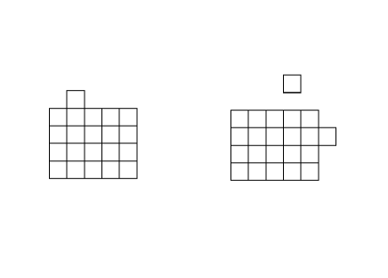
Figure 1: Critical configurations for Glauber and Local Kawasaki dynamics in the case $l_{c}=5$.

Then it was shown (see in particular [31] for Local Kawasaki) that, with $a\in{\cal X}$ the configuration made of $-1$ only ($0$ only) and $b\in{\cal X}$ the configuration made of $+1$ only (1 in $\Lambda\setminus\partial_{-}\Lambda$ and 0 in $\partial_{-}\Lambda$) for Glauber (Local Kawasaki) dynamics, for $\Lambda$ large enough:

(P1)

$b$ is the only one fundamental state, that is the global minimum of the Hamiltonian,

(P2)

$a$ is the only one metastable state in the sense of [29] that is, with

$$\Gamma:=\min\left\{H(a)\vee\max_{e\in\gamma}H(e_{+}):\>\mbox{$\gamma$ is a path from $a$ to $b$}\right\}-H(a)$$ (6.9)

there is, for all $x$ in ${\cal X}\setminus\{a\}$,

$$\Gamma>\min\left\{H(x)\vee\max_{e\in\gamma}H(e_{+}):\>\mbox{$\gamma$ is a path from $x$ to $b$}\right\}-H(x)$$ (6.10)

(P3)

${\cal G}$ has the gate property, i.e., any path that realizes the min-max  (6.9) has to cross ${\cal G}$ and reaches its maximum in ${\cal G}$, so that, in particular,

$$\Gamma=H({\cal G})-H(a)$$ (6.11)

(note that $\Gamma$ depends on $J$ and $h$ or $U$ and $\Delta$ only),

(P4)

if $A$ and $B$ are the two cycles in the sense of Wentzell and Freidlin [7] that are the connected components of $a$ and $b$ in $H^{-1}(]-\infty,H({\cal G})[)$ then

$${\cal G}\subset\partial_{+}A$$ (6.12)

and, by (P2),

$$\forall x\not\in B,\;H(x)>H(a)$$ (6.13)

This is a big amount of information – (P2) includes a control of the global energy landscape – and at this point there are many possible choices for the set ${\cal R}$. Natural choices include

• $A$,

• the connected component of $A$ in $H^{-1}(]-\infty,H({\cal G})])\setminus{\cal G}$,

• $H^{-1}(]-\infty,H({\cal G})])\setminus{B}$,

• larger sets (including for example a small piece of $B$)…

With any of these choices Wentzell-Freidlin theory leads, for all $\delta>0$, to

$$\limsup_{\beta\rightarrow+\infty}\frac{1}{\beta}\ln P_{\mu_{\cal R}}\left(\tau_{{\cal R}^{c}},\tau_{b}\not\in[e^{(\Gamma-\delta)\beta};e^{(\Gamma+\delta)\beta}]\right)<0$$ (6.14)

This does not say much about the existence of our “short time scale” but it is a strong indication that our “long time scale” should be $e^{\Gamma\beta}$. It takes, indeed, for the system initially under $\mu_{\cal R}$, essentially the same (long) time to reach ${\cal R}^{c}$ and $b$, and when the system is in $b$ it is “far from ${\cal R}$”: one can see, using reversibility, that, typically, the system needs at least a time of order

$$e^{(H({\cal G})-H(b))\beta}=e^{(\Gamma+H(a)-H(b))\beta}\gg e^{\Gamma\beta}$$ (6.15)

to go back to ${\cal R}$.

In addition, Wentzell Freidlin theory, leads also to

$$\Gamma = \lim_{\beta\rightarrow+\infty}\frac{1}{\beta}\ln E_{\mu_{\cal R}}\left[\tau_{{\cal R}^{c}}\right]$$ (6.16)

$$= \lim_{\beta\rightarrow+\infty}\frac{1}{\beta}\ln E_{\mu_{\cal R}}\left[\tau_{b}\right]$$ (6.17)

$$= \lim_{\beta\rightarrow+\infty}\frac{1}{\beta}\ln E_{a}\left[\tau_{{\cal R}^{c}}\right]$$ (6.18)

$$= \lim_{\beta\rightarrow+\infty}\frac{1}{\beta}\ln E_{a}\left[\tau_{{b}}\right]$$ (6.19)

We refer to [29] for the derivation of all these results on the basis of (P1)-(P4).

Remarks: i) The pathwise approach on which were based the proofs of (P1)-(P4) gives also the “short time scale”. For example, in the case of the Local Kawasaki dynamics, it is of order $e^{(2\Delta-U)\beta}$ [31].

ii) Equations (6.16)-(6.19) are stronger than (6.14) in the sense that the former imply (with Markov inequality) the upper bound on $\tau_{\cal R}$ and ${\tau_{b}}$ expressed by the latter, while the lower bound on these times is easy to get using reversibility. However it is important to note that (6.16)-(6.19) imply in general an information (of the kind of (P2)) on the global energy landscape. If $a$ does not lie on the bottom of the deepest well (like expressed in (P2)) and can reach, without going in $b$, a well with a depth $\Gamma^{\prime}$ larger than $\Gamma$ with a probability exponentially larger than $e^{-(\Gamma^{\prime}-\Gamma)\beta}$ then (6.16)-(6.19) cannot hold. By contrast, results like (6.14) can be derived by a strictly pathwise approach (see for example [16] on Glauber dynamics in dimension 3) without such kind of information on the global energy landscape.

6.3 Beyond exponential asymptotics

On the basis on (P1)-(P4), potential theory can improve (6.16)-(6.19) beyond exponential asymptotics. Bovier and Manzo did that in [25] and gave the exact asymptotics of $E_{a}[\tau_{b}]$ for Glauber dynamics.

They did so applying (4.29) to the sets $\{a\}$ and $\{b\}$, and, this implied, in particular, giving some estimates on the capacity. As a far as the upper bounds (on the capacity) are concerned, they estimated $C(a,b)$ with

$$C(a,b)\leq C(A,B)$$ (6.20)

where $A$ and $B$ are the two cycles defined in (P4) (by Dirichlet’s principle the conductance is increasing in its arguments). To give a lower bound on the capacity they drop some terms in the Dirichlet form of the variational principle (Rayleigh’s monotonicity law) to get a linear network for which they were able to compute the capacity. This is equivalent to building a linear flow and using Thomson’s principle.

We will use a slightly different strategy: we will apply (4.29) directly to our cycles $A$ and $B$. But before doing that we have to pass through a little algebra to link the study of our continuous time Markov process $X$ to that of the discrete time random walks $\xi$ we dealt with in the previous sections.

Observe that the generator $L$ defined in (6.2) cannot be written in the form that ${\cal L}$ assumed in (2.9): given $x\in{\cal X}$ the sum on $y\sim x$ of the rates

$$\lambda(x,y):=\exp\left\{-\beta[H(y)-H(x)]_{+}\right\}$$ (6.21)

is in general larger than one. But it is certainly smaller than

$$N:=\left\{\begin{array}[]{l}\mbox{number of sites in $\Lambda$ for Glauber}\\ \mbox{number of bonds inside $\Lambda\setminus\partial_{-}\Lambda$ and sites in $\partial_{-}\Lambda$ for Kawasaki}\end{array}\right.$$ (6.22)

We define then the network $({\cal X},c)$ with, for all $x$ and $y$ in ${\cal X}$,

$$c(x,y):=\left\{\begin{array}[]{ll}0&\mbox{if $y\neq x$ and $y\not\sim x$}\\ \frac{\mu(x)\lambda(x,y)}{N}&\mbox{if $y\neq x$ and $y\sim x$}\\ \mu(x)-\sum_{\stackrel{{\scriptstyle\scriptstyle y\sim x}}{{y\neq x}}}\frac{\mu(x)\lambda(x,y)}{N}&\mbox{if $y=x$}\end{array}\right.$$ (6.23)

Since, for all $x$ in ${\cal X}$,

$$\sum_{y\in{\cal X}}c(x,y)=\mu(x)$$ (6.24)

the random walk $\xi$ associated with $({\cal X},c)$ is reversible with respect to $\mu$. Its generator is defined by

$${\cal L}_{x}f:=\sum_{y\in{\cal X}}\frac{c(x,y)}{\mu(x)}(f(y)-f(x))=\sum_{y\sim x}\frac{\lambda(x,y)}{N}(f(y)-f(x))=\frac{1}{N}L_{x}f$$ (6.25)

Recall that we called “generator of a discrete time Markov chain $\xi$” that of the continuous time process that updates its position at each ring of a Poissonian clock of intensity 1 according to the transition probabilities of $\xi$. Denoting by $\tilde{\xi}$ this continuous time process (6.25) means that $\tilde{\xi}$ is nothing but the rescaled process $X$: $\tilde{\xi}$ behaves like $X$ except for the fact that it is $N$ times slower.

As a consequence

$$E_{\nu_{A}}[\tau_{B}(X)]=\frac{1}{N}E_{\nu_{A}}[\tau_{B}(\tilde{\xi})]=\frac{1}{N}E_{\nu_{A}}[\tau_{B}(\xi)]$$ (6.26)

and (4.29) gives

$$E_{\nu_{A}}[\tau_{B}(X)]=\frac{1}{NC(A,B)}\sum_{x\not\in B}\mu(x)P_{x}(\tau_{A}<\tau_{B})$$ (6.27)

where we have to recall that the conductances that are involved in the computation of $C(A,B)$ are defined in (6.23) and depend on $N$ too.

By (6.13) the last sum in (6.27) is equivalent to $\mu(a)$ and, in the case of the 2-dimensional Glauber dynamics, it turns out that for all $g$ in ${\cal G}$, $A\cup\{g\}\cup B$ is a connected set, while for all distinct $g$, $g^{\prime}$ in ${\cal G}$, $g$ and $g^{\prime}$ are not connected. These two properties make then the capacity in (6.27) quite easy to estimate. Indeed, we first note that for all $x\neq y$ with $x\sim y$,

$$c(x,y)=\frac{\mu(x)\lambda(x,y)}{N}=\frac{\exp\{-\beta(H(x)\vee H(y))\}}{NZ}$$ (6.28)

This implies that, for any function $f$ on ${\cal X}$ that takes its values in $[0,1]$, is equal to $1$ on $A$ and to $0$ on $B$, all the terms in the Dirichlet from $D(f)$ that involve a node beyond the energy level $H({\cal G})$ are exponentially smaller than $D(f)$, and, using the gate property of ${\cal G}$ and the fact that for all $g$ in ${\cal G}$, $A\cup\{g\}\cup B$ is a connected set, we conclude that the $C(A,B)$ is equivalent to the capacity of the pair $(A,B)$ in the network $(A\cup{\cal G}\cup B,c)$. In this network a fraction $2/l_{c}$ of the nodes in ${\cal G}$ have only one edge towards $A$ and one edge towards $B$, while the other nodes have only one edge towards $A$ and two edges towards $B$.

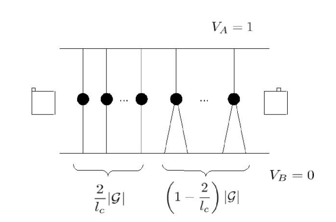
Figure 2: The network $(A\cup{\cal G}\cup B,c)$.

All these edges have the same conductance

$$\bar{c}=\frac{\exp\{-\beta H({\cal G})\}}{NZ}$$ (6.29)

and we get

$$C(A,B)\sim\frac{\frac{2}{l_{c}}|{\cal G}|}{\frac{1}{\bar{c}}+\frac{1}{\bar{c}}}+\frac{\left(1-\frac{2}{l_{c}}\right)|{\cal G}|}{\frac{1}{\bar{c}}+\frac{1}{2\bar{c}}}=\frac{(2l_{c}-1)|{\cal G}|{\exp\{-\beta H({\cal G})\}}}{3l_{c}{NZ}}$$ (6.30)

We conclude, using (6.11),

$$E_{\nu_{A}}[\tau_{B}(X)]\sim\frac{{3l_{c}{Z}}\mu(a)}{{(2l_{c}-1)|{\cal G}|{\exp\{-\beta H({\cal G})\}}}}=\frac{{3l_{c}e^{\Gamma\beta}}}{(2l_{c}-1)|{\cal G}|}$$ (6.31)

From this we get the same estimate on $E_{a}[\tau_{b}]$. Here is the logic of the argument. The probability $\nu_{A}$ is concentrated on $A$ that is a cycle of depth $\Gamma$, as a consequence the system will typically reach $a$ in a time exponentially smaller than $e^{\Gamma\beta}$ before going to $B$. But $B$ is a cycle with internal resistance smaller than $\Gamma$ ($a$ is the only one metastable state), hence, after reaching $B$ the system will typically go to $b$ in a time exponentially smaller than $e^{\Gamma\beta}$. This leads, for any small enough $\delta>0$, to

$$E_{a}[\tau_{b}]+o(e^{(\Gamma-\delta)\beta})=E_{\nu_{A}}[\tau_{B}(X)]\sim\frac{{3l_{c}e^{\Gamma\beta}}}{(2l_{c}-1)|{\cal G}|}$$ (6.32)

and

$$E_{a}[\tau_{b}]\sim\frac{{3l_{c}e^{\Gamma\beta}}}{(2l_{c}-1)|{\cal G}|}$$ (6.33)

To put the argument properly you have to quantify the probability of “atypical behaviours” to control the expectations, and this, knowing (P1)-(P4), is elementary classical Wentzell-Freidlin theory.

With (6.33) everything boils down to the computation of the number of critical configurations. For the 2-dimensional finite volume Glauber dynamics we find

$$|{\cal G}|=4l_{c}|\Lambda|$$ (6.34)

(there are $|\Lambda|$ choices for the south-west corner of the quasi-square, 2 choices for its orientation and $2l_{c}$ choices for the position of the protuberance). We refer to [25] for the study of the dynamics in higher dimension.

For Local Kawasaki the situation is more complex: first ${\cal G}$ (that is not uniquely defined) is not so simple, second the electrical network that connects $A$ and $B$ is “stretched” and much more intricate. But the same method can be applied, $C(A,B)$ can be estimated via our two variational principles, and, once again, everything is reduced to some computation of $|{\cal G}|$. This is the difficult point of [34] that gives sharp asymptotics of $E_{a}[\tau_{b}]$ for this model in dimensions 2 and 3.

6.4 Large volume dynamics

Glauber and Kawasaki dynamics in large volume are defined as continuous time Markov chains $X$ on the space ${\cal X}$ of the configurations made on -1 and +1 (Glauber) or 0 and 1 (Kawasaki) on the d-dimensional discrete torus $\Lambda_{\beta}$ of volume

$$|\Lambda_{\beta}|=e^{\Theta\beta}$$ (6.35)

(we round off large integers). They are defined by a Metropolis algorithm associated with the Hamiltonian

$$H:\sigma\in{\cal X}\mapsto-\frac{1}{2}\sum_{\stackrel{{\scriptstyle\scriptstyle\{i,j\}\subset\Lambda_{\beta}}}{{\scriptstyle d_{1}(i,j)=1}}}J\sigma_{i}\sigma_{j}-\frac{1}{2}\sum_{i\in\Lambda}h\sigma_{i}$$ (6.36)

for Glauber dynamics ($y\sim x$ in (6.2) has the same signification as that of the finite volume dynamics), and

$$H:\eta\in{\cal X}\mapsto\sum_{\stackrel{{\scriptstyle\scriptstyle\{i,j\}\subset\Lambda_{\beta}}}{{\scriptstyle d_{1}(i,j)=1}}}-U\eta_{i}\eta_{j}$$ (6.37)

for Kawasaki dynamics ($y\sim x$ in (6.2) now simply means that $y$ is obtained from $x=\eta\in{\cal X}$ by exchanging the value of $\eta$ between two nearest neighbour sites $i$ and $j$ in $\Lambda_{\beta}$). We will assume

$$\Theta<\Gamma$$ (6.38)

where $\Gamma$ is the energy barrier defined in the local version of the dynamics.

In large volume, we lose much of the tools inherited from Wentzell and Freidlin. Nevertheless many kind of restricted ensembles have been individuated for Glauber dynamics even in infinite volume or at fixed temperature ([18], [21]). It is not so for conservative dynamics: as far as I know there are still only unpublished results ([39], [40]) that prove the desired properties of a set ${\cal R}$ in large volume with $d=2$. But with the tools of potential theory Bovier, den Hollander and Spitoni [37] computed sharp asymptotics on some hitting times that give very strong indication that the set ${\cal R}$ defined as the set of configurations for which there are no more than $l_{c}(l_{c}-1)+1$ particles inside each square box of volume smaller than $L^{2}_{\beta}$ with

$$L^{2}_{\beta}:=e^{({\Delta}-\delta_{\beta})\beta}\mbox{ with $\delta_{\beta}=o(1)$ and $\frac{1}{\beta}=o(\delta_{\beta})$}$$ (6.39)

can be associated with a metastable restricted ensemble. They also gave analogous results for Glauber dynamics. I refer to [37] for precise statements. Here I just want to make a few comments on the method.

The central idea is to apply (4.29). We have then four main questions to deal with:

• How should we choose $A$ and $B$?

• How can we estimate the capacity $C_{A,B}$?

• How can we estimate the mean potential $\mu(V_{A,B})$?

• How can we link the expectation starting from the harmonic measure $E_{\nu_{A}}$ with the expectation starting from the restricted ensemble $E_{\mu_{\cal R}}$?

The ideal choices for $A$ and $B$ would be $A=\{a\}$ for any $a$ in ${\cal R}$ and $B={\cal R}^{c}$, then $B$ in a sequence of sets that go far away from ${\cal R}$. If we were able to prove that for such choices $E_{\nu_{A}}[\tau_{B}]$ has a divergent asymptotic (in exponential of $\beta$) that does not depend on $A$ and $B$, we would not have our “short time scale” but, since lower bounds on typical exit time are generally easy to get by reversibility, the problem would essentially be solved. In particular Q4 would have a trivial answer. But choosing for $A$ a singleton $\{a\}$ makes in general Q2 and Q3 extremely difficult to answer. Indeed we always have, see (2.51),

$$C(a,B)\leq\mu(a)$$ (6.40)

and $C(a,B)$ turns out to be super-exponentially small. This would also imply a sharp control on $\mu(V_{A,B})$ that is extremely difficult to get: we are indeed on the discrete version of a continuous Dirichlet problem without solution on a bounded domain. In conclusion $A$ has to be “big enough”. As far as the choice of $B$ is concerned we remain for a while on our ideal choice.

For a big enough $A$, Q2 is the easiest to answer: we can make use of our two variational principles. Actually Bovier, den Hollander and Spitoni made use of a more elaborated variational principle on the effective resistance that is due to Berman and Konsowa [8].

Q3 is in general more difficult to answer, since we do not have a variational principle on the potential. Sometimes, like in [22], [25], one can reduce an estimate on a potential to an estimate on capacities with the following

Lemma 6.4.1

For all $x$ outside of $A$ and $B$, disjoint sets, it is

$$P_{x}(\tau_{A}<\tau_{B})\leq\frac{C_{x,A}}{C_{x,B}}$$ (6.41)

Proof:

$$P_{x}(\tau_{A}<\tau_{B}) = \quad P_{x}(\tau_{A}<\tau_{B}|\tau_{x}^{+}>\tau_{A\cup B})P_{x}(\tau_{x}^{+}>\tau_{A\cup B})$$ (6.42)

$$+\;P_{x}(\tau_{A}<\tau_{B}|\tau_{x}^{+}<\tau_{A\cup B})P_{x}(\tau_{x}^{+}<\tau_{A\cup B})$$

The first term in this sum is bounded from above by

$$P_{x}(\tau^{+}_{x}>\tau_{A}|\tau_{x}^{+}>\tau_{A\cup B})P_{x}(\tau_{x}^{+}>\tau_{A\cup B})=P_{x}(\tau^{+}_{x}>\tau_{A})$$ (6.43)

while the second term is equal to

$$P_{x}(\tau_{A}<\tau_{B})P_{x}(\tau_{x}^{+}<\tau_{A\cup B})=P_{x}(\tau_{A}<\tau_{B})(1-P_{x}(\tau_{x}^{+}>\tau_{A\cup B}))$$ (6.44)

Solving in $P_{x}(\tau_{A}<\tau_{B})$ we get

$$P_{x}(\tau_{A}<\tau_{B})\leq\frac{P_{x}(\tau^{+}_{x}>\tau_{A})}{P_{x}(\tau_{x}^{+}>\tau_{A\cup B})}\leq\frac{P_{x}(\tau^{+}_{x}>\tau_{A})}{P_{x}(\tau_{x}^{+}>\tau_{B})}=\frac{C_{x,A}}{C_{x,B}}$$ (6.45)

$\Box$

Unfortunately, single points in large volume have not enough mass for this to be useful (see above). Potential are difficult to estimate (in [39], [40] this kind of estimates involve a complex renormalization procedure) but we still have the trivial estimate

$$V_{A,B}\leq{\tt 1\tt l}_{B^{C}}$$ (6.46)

On the model of our estimates of Section 6.3, what is needed is an estimate of the kind

$$\mu(V_{A,B})\sim\mu({\cal R})$$ (6.47)

and this is given by (6.46) only if $B$ is not “too far” from ${\cal R}$.

Denoting by $A_{n}$ the subset of ${\cal R}$ such that there are no more than $n\leq l_{c}(l_{c}-1)+1$ particles inside each square box of volume smaller than $L^{2}_{\beta}$, by $n_{0}$ the smallest $n$ for which

$$\mu_{{\cal{}_{R}}}(A_{n})\sim 1$$ (6.48)

and, for all $l\geq l_{c}$, by $B_{n}$ the subset of ${\cal R}^{c}$ of the configurations $\eta$ in ${\cal X}$ that contain (as subset of $\Lambda_{\beta}$) a square of side length $l$, Bovier, den Hollander and Spitoni give the sharp asymptotic

$$\forall n\in[n_{0},lc(lc-1)+1],\;\forall l\in[l_{c},2l_{c}-1],\;E_{\nu_{A_{n}}}[\tau_{B_{l}}]\sim\frac{3\Delta\beta e^{\Gamma\beta}}{4\pi l_{c}^{2}(l_{c}^{2}-1)|\Lambda_{\beta}|}$$ (6.49)

Postponing the discussion on Q4, this essentially gives us our long time scale (beyond exponential asymptotics!) and the constraint $l\leq 2l_{c}-1$ is here just as a consequence of the difficulties that are encountered for estimating potentials. However, in the case of Glauber dynamics and as far as I understand, one could remove this constraint by an attractiveness argument that was used in the previous works in large volume and makes locally available the tools of Wentzell and Freidlin theory (just like we used it in Section 6.3 in alternative to Lemma 6.4.1).

One of the main strength of (6.49) is that it gives asymptotics that do not depend on $n$. One could have thought that the harmonic measure $\nu_{A}$ being concentrated on the internal border of $A$ would have introduced a bias. It is not so and the reason for this is probably the same that led us from the beginning to associate with ${\cal R}$ the restricted ensemble $\mu_{\cal R}$ that is also the reversible and invariant measure for the dynamics restricted to ${\cal R}$: for any “good” ${\cal R}$ the system should typically relax in a short time scale to $\mu_{\cal R}$. Actually, Q4 raises a problem of convergence to (metastable) equilibrium. This is the object of the next and final section.

7 Application to convergence to equilibrium

7.1 Spectral gap

For an extended covering of convergence to equilibrium we refer to [19] and [33]. Here we just indicate how the objects we discussed above link to the argument. We recall that for $\xi$ Markov chain on a finite state space ${\cal X}$ with transition probability matrix $M$, $\xi$ is reversible with respect to the probability measure $\mu$ if and only if $M$ is a self-adjoint operator on $\ell^{2}(\mu)$. In this case $M$ has only real eigenvalues

$$1=\lambda_{0}>\lambda_{1}\geq\dots\geq\lambda_{N-1}\geq-1$$ (7.1)

and $\lambda_{N-1}>-1$ if and only if $\xi$ is aperiodic. In this case the rate of convergence to equilibrium in $\ell^{2}(\mu)$ is governed by

$$\bar{\lambda}:=\max\{|\lambda_{1}|;|\lambda_{N-1}|\}$$ (7.2)

If $\bar{\lambda}\neq\lambda_{1}$ then the transition matrix $(M+I)/2$ of the associated lazy chain $\xi^{\prime}$ has only positive eigenvalues and a rate of convergence of the same order. We will then assume that $\xi$ itself is a reversible and ergodic Markov chain with a transition matrix $M$ the eigenvalues of which are all positive. In this case the rate of convergence of $\xi$ in $\ell^{2}(\mu)$ is given by the spectral gap

$$\lambda:=1-\lambda_{1}$$ (7.3)

that is the smallest non-zero eigenvalue of

$$I-M=-{\cal L}$$ (7.4)

or, equivalently,

$$\lambda:=\min_{f\in(Ker{\cal L})^{\bot}}\frac{\langle f,(-{\cal L})f\rangle_{\mu}}{\langle f,f\rangle_{\mu}}$$ (7.5)

The numerator in this variational principle is

$$\langle f,(-{\cal L})f\rangle_{\mu} = \sum_{x}\mu(x)f(x)\left(f(x)-\sum_{y}p(x,y)f(y)\right)$$ (7.6)

$$= \sum_{x}\mu(x)f(x)\sum_{y}p(x,y)(f(x)-f(y))$$ (7.7)

$$= \frac{1}{2}\sum_{x,y}\mu(x)p(x,y)(f(x)-f(y))^{2}$$ (7.8)

$$= {\cal D}(f)$$ (7.9)

In addition, the kernel of ${\cal L}$ is the one-dimensional subspace of $\ell^{2}(\mu)$ that contains all the constant functions, and the orthogonal projection of any $f$ on this subspace is the constant function $\mu(f)$. As a consequence one can extend the minimum in (7.5) as a minimum on all the non-constant functions replacing $f$ by $f-\mu(f)$, and this gives

$$\lambda=\min_{{\rm Var}(f)\neq 0}\frac{{\cal D}(f)}{{\rm Var}(f)}$$ (7.10)

Any test function $f$ gives an upper bound on the spectral gap. Restricting the minimum to characteristic functions we get

$$\lambda \leq \min_{A\subset{\cal X}}\frac{\sum_{e\in\partial A}c(e)}{\mu(A)(1-\mu(A))}$$ (7.11)

$$\leq 2\min_{\mu(A)\leq\frac{1}{2}}\frac{C(A,A^{c})}{\mu(A)}\;=\;2I$$ (7.12)

where the isoperimetric constant $I$ is defined by the last equation.

Actually $I$ gives also a lower bound on $\lambda$:

Lemma [Cheeger]:

$$\frac{I^{2}}{2}\leq\lambda\leq 2I$$ (7.13)

We refer to [19] for the proof where it is shown that a lower bound on $I$ expresses an $\ell^{1}$ version of a Poincaré inequality. A Poincaré inequality is an inequality of the form

$$\forall f\in\ell^{2}(\mu),\;{\rm Var}(f)\leq\kappa{\cal D}(f)$$ (7.14)

and is equivalent to a lower bound on the spectral gap.

If instead of restricting the minimum to characteristic function that are particular cases of equilibrium potential we restrict the minimum to general equilibrium potential $V_{A,B}$, we get

$$\lambda \leq \min_{A\cap B=\emptyset}\frac{C(A,B)}{{\rm Var}(V_{A,B})}$$ (7.15)

$$\leq \min_{A\cap B=\emptyset}\frac{C(A,B)}{\mu(A)\mu(B)}$$ (7.16)

Indeed,

$${\rm Var}(V_{A,B}) = \frac{1}{2}\sum_{x,y}\mu(x)\mu(y)[V_{A,B}(x)-V_{A,B}(y)]^{2}$$ (7.17)

$$\geq \frac{1}{2}\sum_{x,y\in A\cup B}\mu(x)\mu(y)$$ (7.18)

$$= \mu(A)\mu(B)$$ (7.19)

In the metastable situation, when we have $a$, $b$, ${\cal G}$ that satisfy (P1)-(P4) of Section 6.2 this gives

$$\lambda\leq\frac{C(A,B)}{\mu(A)\mu(B)}\sim\frac{C(A,B)}{\mu(A)}\sim\frac{1}{E_{\nu_{A}}[\tau_{B}]}\sim\frac{1}{E_{a}[\tau_{b}]}$$ (7.21)

We prove in the next section that this is the correct asymptotics.

7.2 Lower bounds for the spectral gap

We start with an easy estimate. Given $f\in\ell^{2}(\mu)$ we have for any $x$ and $y$ in ${\cal X}$, by bilinearity of ${\cal D}$ and Dirichlet’s principle,

$$[f(x)-f(y)]^{2}\leq R(x,y)D(f)$$ (7.22)

Multiplying by $\mu(x)\mu(y)$ and summing on all $x$ and $y$ we get a Poincaré inequality

$${\rm Var}(f)\leq\frac{1}{2}\left(\sum_{x,y}\mu(x)\mu(y)R(x,y)\right)D(f)$$ (7.23)

In the metastable situation with (P1)-(P4) one can estimate the effective resistance between $x$ and $y$ by building a linear (i.e., without ramifications) unitary flow from $x$ to $y$ with $H(x)\geq H(y)$ to get

$$\mu(x)\mu(y)R(x,y)=O\left(\mu(y)e^{\beta\Gamma_{x,y}}\right)$$ (7.24)

with $\Gamma_{x,y}$ the energy barrier between $x$ and $y$ defined by (6.9) with $x$ and $y$ in place of $a$ and $b$. Since

$$\mu(a)\mu(b)R(a,b)\sim\mu(a)R(a,b)\sim E_{a}[\tau_{b}]$$ (7.25)

is logarithmically equivalent to $e^{\Gamma}\beta$, we get, with (P1) and (P2),

$$\frac{1}{\lambda}\leq E_{a}[\tau_{b}](1+o(1))$$ (7.26)

and, together with (7.21),

$$\frac{1}{\lambda}\sim E_{a}[\tau_{b}]$$ (7.27)

In [22] Bovier, Eckhoff, Gayrard and Klein prove such a relation for all the “low-lying eigenvalues” of the generator. In addition they prove that associated eigenvectors are equivalent to some equilibrium potentials.

Better bounds. In many situations our previous Poincaré inequality is however a bad one. This is because for different $x$ and $y$ the equality in (7.22) is in general realised by very different $f$. To improve this bound we modify the network in a specific way for each $x$ and $y$. If we increase the conductance of the edges that are more charged by $i_{x,y}$ then we can decrease the resistance in (7.22). After that we will have to reconstruct a Poincaré inequality on the global network on the basis of these different inequalities in different networks. This may give good bounds if the currents in the different modified networks tend to use different edges. To put it formally, we associate with each $(x,y)$ in ${\cal X}^{2}$ a unitary flow $\phi_{x,y}$ and a weight function

$$w_{x,y}:e\in{\cal E}\mapsto w_{x,y}(e)\in[0;+\infty[$$ (7.28)

such that, for all $e$ in ${\cal E}$,

$$(\phi_{x,y}(e)=0)\Rightarrow(w_{x,y}(e)=0)$$ (7.29)

Interesting choices are

$$w^{1}_{x,y} := 1-{\tt 1\tt l}_{\{0\}}\circ\phi_{x,y}$$ (7.30)

$$w^{2}_{x,y} := |\phi_{x,y}|$$ (7.31)

$$w^{3}_{x,y} := |r\phi_{x,y}|$$ (7.32)

$$w^{4}_{x,y} := r\phi^{2}_{x,y}$$ (7.33)

Then we denote by ${\cal D}_{x,y}$ the Dirichlet form associated with the network obtained by replacing $c$ with $cw_{x,y}$ and restriction to the connected component that contain both $x$ and $y$. In particular we have

$${\cal D}_{x,y}(\phi_{x,y})=\sum_{e:\phi_{x,y}(e)>0}\frac{r(e)}{w_{x,y}(e)}\phi^{2}_{x,y}(e)$$ (7.34)

Now using both our variational principles we have

$$|f(x)-f(y)|^{2} \leq {\cal D}_{x,y}(\phi_{x,y}){\cal D}_{x,y}(f)$$ (7.35)

$$= {\cal D}_{x,y}(\phi_{x,y})\sum_{e:\phi_{x,y}(e)>0}c(e)w_{x,y}(e)|-\nabla_{e}f|^{2}$$ (7.36)

Multiplying by $\mu(x)\mu(y)$ and summing on all $x$ and $y$ we get

$${\rm Var}(f) \leq \frac{1}{2}\sum_{x,y}\mu(x)\mu(y){\cal D}_{x,y}(\phi_{x,y})\sum_{\stackrel{{\scriptstyle\scriptstyle e\in{\cal E}}}{{\phi_{x,y}(e)>0}}}\!\!\!c(e)w_{x,y}(e)|-\nabla_{e}f|^{2}$$ (7.37)

$$= \frac{1}{2}\sum_{e\in{\cal E}}c(e)|-\nabla_{e}f|^{2}\sum_{\stackrel{{\scriptstyle\scriptstyle{x,y}\in{\cal X}}}{{\phi_{x,y}(e)>0}}}\!\!\!\mu(x)\mu(y)w_{x,y}(e){\cal D}_{x,y}(\phi_{x,y})$$ (7.38)

$$\leq {\cal D}(f)\times\max_{e\in{\cal E}}\!\!\!\sum_{\stackrel{{\scriptstyle\scriptstyle x,y\in{\cal X}}}{{\phi_{x,y}(e)>0}}}\!\!\!\mu(x)\mu(y)w_{x,y}(e){\cal D}_{x,y}(\phi_{x,y})$$ (7.39)

This Poincaré inequality gives

Lemma 7.2.1

For any family of unitary flow $\phi_{x,y}$ from $x$ to $y$ and $w_{x,y}$ that satisfies (7.28) and (7.29) we have

$$\frac{1}{\lambda}\leq\max_{e\in{\cal E}}\!\!\!\sum_{\stackrel{{\scriptstyle\scriptstyle{x,y}\in{\cal X}}}{{\phi_{x,y}(e)>0}}}\!\!\!\mu(x)\mu(y)w_{x,y}(e){\cal D}_{x,y}(\phi_{x,y})$$ (7.40)

With $w=w^{1}$ we get

$$\frac{1}{\lambda}\leq\max_{e\in{\cal E}}\!\!\!\sum_{\stackrel{{\scriptstyle\scriptstyle{x,y}\in{\cal X}}}{{\phi_{x,y}(e)>0}}}\!\!\!\mu(x)\mu(y){\cal D}(\phi_{x,y})$$ (7.41)

With $w=w^{2}$ and $\phi_{x,y}$ built as a family of linear flows that is

$$\phi_{x,y}(e)={\tt 1\tt l}_{\gamma(x,y)}(e)-{\tt 1\tt l}_{\gamma(x,y)}(-e)$$ (7.42)

with $\gamma(x,y)$ simple path from $x$ to $y$ we get

$$\frac{1}{\lambda}\leq\max_{e\in{\cal E}}\!\!\!\sum_{\stackrel{{\scriptstyle\scriptstyle{x,y}\in{\cal X}}}{{e\in\gamma(x,y)}}}\mu(x)\mu(y)\sum_{e^{\prime}\in\gamma(x,y)}r(e^{\prime})$$ (7.43)

and this is Diaconis and Stroock’s estimate [9].

With $w=w^{3}$ and $\phi_{x,y}$ built like previously we get

$$\frac{1}{\lambda}\leq\max_{e\in{\cal E}}\!\!\!\sum_{\stackrel{{\scriptstyle\scriptstyle x,y\in{\cal X}}}{{e\in\gamma(x,y)}}}\mu(x)\mu(y)r(e)|\gamma(x,y)|$$ (7.44)

that is one of Sinclair’s estimates in [14], while in the general case we get

$$\frac{1}{\lambda}\leq\max_{e\in{\cal E}}\!\!\!\sum_{\stackrel{{\scriptstyle\scriptstyle{x,y}\in{\cal X}}}{{\phi_{x,y}(e)>0}}}\!\!\!\mu(x)\mu(y)r(e)\phi_{x,y}(e)\sum_{\stackrel{{\scriptstyle\scriptstyle e^{\prime}\in{\cal E}}}{{\phi_{x,y}(e^{\prime})>0}}}\!\!\!\phi_{x,y}(e^{\prime})$$ (7.45)

that is essentially equivalent to Sinclair’s formula for “multicommodity flows”, actually strictly equivalent if $\phi_{x,y}$ is built (like usually it is) as a flow of geodesic paths.

With $w=w^{4}$ we get

$$\frac{1}{\lambda}\leq\max_{e\in{\cal E}}\!\!\!\sum_{\stackrel{{\scriptstyle\scriptstyle x,y\in{\cal X}}}{{\phi_{x,y}(e)>0}}}\!\!\!\mu(x)\mu(y)r(e)\phi^{2}_{x,y}(e)\Big{|}\Big{\{}e^{\prime}\in{\cal E}:\>\phi_{x,y}(e^{\prime})>0\Big{\}}\Big{|}$$ (7.46)

Previous choices have proven their efficiency but at the time of sending these notes I did not have that of seriously checking the advantages of this last choice.

7.3 Mixing time

A stronger notion of convergence to equilibrium is that of the mixing time

$$\tau_{1}:=\inf\left\{t\geq 0:\>\max_{x\in{\cal X}}\left\|P_{x}^{t}-\mu\right\|_{TV}\leq\frac{1}{e}\right\}$$ (7.47)

where

$$\left\|P_{x}^{t}-\mu\right\|_{TV}:=\max_{A\in{\cal X}}\Big{|}P_{x}(\xi(t)\in A)-\mu(A)\Big{|}$$ (7.48)

is the total variation distance that, maximized over $x$, decays exponentially [33]. Since an exponential decay of the total variation distance implies an exponential decay at the same rate (at least) in $\ell^{2}(\mu)$, we have

$$-\ln(1-\lambda)\geq\frac{1}{\tau_{1}}$$ (7.49)

In our metastable situation, since the equilibrium measure is essentially concentrated on $\{b\}$, the study of the convergence to equilibrium should be essentially an hitting time problem. The coupling argument used in [32], turns this intuition in a rigorous estimate of the mixing time. For any ergodic and aperiodic Markov chain $\xi$ and any coupling $(X,Y)$ with marginals following the law of $\xi$ we have, for all $t\geq 0$ [33]

$$\max_{x\in{\cal X}}\left\|P_{x}^{t}-\mu\right\|_{TV}\leq\max_{x,y\in{\cal X}}P_{x,y}(\tau_{c}>t)$$ (7.50)

with

$$\tau_{c}:=\inf\{t\geq 0:\>X(t)=Y(t)\}$$ (7.51)

In our metastable situation, we can then obtain sharp estimates on the basis of the exponential law:

Proposition 7.3.1

For a continuous time Markov chain built on a Metropolis algorithm at low temperature $\beta^{-1}$ on a finite state space ${\cal X}$ and such that (P1)-(P4) hold, the random variables

$$\theta_{b}:=\frac{\tau_{b}}{E[\tau_{b}]}\quad\mbox{and}\quad\theta_{B}:=\frac{\tau_{B}}{E[\tau_{B}]}$$ (7.52)

converge in law under $P_{a}$ towards an exponential random time of mean 1 as $\beta$ goes to infinity.

This kind of result goes back at least to Cassandro, Galves, Olivieri and Vares’ work [5]. The nice following proof is adapted from [29]. The argument works the same in much more general situation: as long as one can talk about metastable single states.

Proof: We prove the result for $\theta_{B}$: the same proof works for $\theta_{b}$. Since

$$T\geq 0\mapsto P_{a}(\tau_{B}>T)$$ (7.53)

is a non-increasing continuous function taht goes from 1 to 0, we can define

$$T_{B}:=\min\left\{T\geq 0:\>P_{a}(\tau_{B}>T)=\frac{1}{e}\right\}$$ (7.54)

For all positive $s$ we define also

$$\tau^{*}:=\inf\Big{\{}t\geq sT_{B}:\>X(t)\in\{a\}\cup B\Big{\}}$$ (7.55)

With

$$R:=e^{(\tilde{\Gamma}+\delta_{0})\beta}$$ (7.56)

where $\tilde{\Gamma}$ is the internal resistance of $B^{c}$, that is the maximal energy barrier under $\Gamma$ between two states $x$ in $B^{c}$ and $y$ in $B^{c}\cup\partial_{+}(B^{c})$, and $\delta_{0}>0$ is such that $\tilde{\Gamma}+\delta_{0}<\Gamma$, we know, by classical Wentzell-Freidlin theory, that the probability of $\tau^{*}-sT_{B}$ being larger than $R$ is super exponentially small ($SES$), that is

$$\limsup_{\beta\rightarrow+\infty}\frac{1}{\beta}\ln P_{a}(\tau^{*}-sT_{B}\geq R)=-\infty$$ (7.57)

For all positive $t$, if $\tau_{B}$ is larger than $(s+t)T_{B}$ then $X$ will be outside $B$ on the whole intervals

$$I=[0,sT_{B}]\quad\mbox{and}\quad J=[\tau^{*}\wedge(s+t)T_{B},(s+t)T_{B}]$$ (7.58)

Since, up to a $SES$ event, $J$ is longer than $tT_{B}-R$,

$$P_{a}(\tau_{B}>(s+t)T_{B})\leq P_{a}(\tau_{B}>sT_{B})P_{a}(\tau_{B}>tT_{B}-R)+SES$$ (7.59)

If $X$ stays outside $B$ on

$$I=[0,\tau^{*}]\quad\mbox{and}\quad J=[\tau^{*},\tau^{*}+tT_{B}]$$ (7.60)

then $\tau_{B}$ will be larger than $(s+t)T_{B}$. Since, up to a $SES$ event, $I$ is shorter than $tT_{B}+R$,

$$P_{a}(\tau_{B}>sT_{B}+R)P_{a}(\tau_{B}>tT_{B})-SES\leq P_{a}(\tau_{B}>(s+t)T_{B})$$ (7.61)

By classical Wentzell-Freidlin theory we have also, for all $\delta>0$,

$$\limsup_{\beta\rightarrow+\infty}\frac{1}{\beta}\ln P_{a}(\tau_{B}<e^{(\Gamma-\delta)\beta})<0$$ (7.62)

so that

$$R=o(T_{B})$$ (7.63)

and, by (7.59), for all large enough $\beta$,

$$P_{a}(\tau_{B}>(s+t)T_{B})\leq P_{a}(\tau_{B}>sT_{B})P_{a}(\tau_{B}>(t-1)T_{B})+SES$$ (7.64)

For all $n=2k$, we get then, by induction on $k\geq 2$ and using (7.54)

$$P_{a}(\tau_{B}>nT_{B})\leq e^{-\frac{n}{2}\beta}+nSES$$ (7.65)

and the tightness of $(\bar{\theta}_{\beta})_{\beta>0}$ with

$$\bar{\theta}_{\beta}:=\frac{\tau_{B}}{T_{B}}$$ (7.66)

By Alaoglu’s theorem and diagonal extraction there is a diverging sequence $(\beta_{k})_{k\geq 0}$ such that $\bar{\theta}_{\beta_{k}}$ converges in law towards a random variable $\hat{\theta}$, for which, with (7.59), (7.61) and (7.63), we have necessarily

$$P\left(\hat{\theta}>s+t\right)=P\left(\hat{\theta}>s\right)P\left(\hat{\theta}>t\right)$$ (7.67)

for all $s$ and $t$ outside ${\cal A}$, set of $\hat{\theta}$’s atoms. Since ${\cal A}$ is a countable set, so is ${\mathbb{Q}}{\cal A}$ and there is some $x>0$ such that

$$x{\mathbb{Q}}\cap{\cal A}\subset\{0\}$$ (7.68)

By density of $x{\mathbb{Q}}$ and monotonicity of the repartition function we conclude that $\hat{\theta}$ follows an exponential law. By (7.54) this can only be that of mean 1 and we get, for all $t>0$,

$$\lim_{\beta\rightarrow+\infty}P_{a}\Big{(}\tau_{B}>tT_{B}\Big{)}=e^{-t}$$ (7.69)

In addition, by dominated convergence,

$$\lim_{\beta\rightarrow+\infty}\frac{E_{a}[\tau_{B}]}{T_{B}}=\lim_{\beta\rightarrow+\infty}\int_{0}^{+\infty}P_{a}(\bar{\theta}_{\beta}>t)dt=\int_{0}^{+\infty}e^{-t}dt=1$$ (7.70)

Now for $t>0$ and any $\epsilon>0$ we choose $\gamma>1$ such that

$$e^{-t}-\epsilon<\frac{1}{\gamma}e^{-\gamma t}<{\gamma}e^{-\frac{t}{\gamma}}<e^{-t}+\epsilon$$ (7.71)

For $\beta$ large enough we have, on the one hand

$$P_{a}(\theta_{B}>t)\leq P_{a}\left(\tau_{B}>\frac{tT_{B}}{\gamma}\right)\leq{\gamma}e^{-\frac{t}{\gamma}}\leq e^{-t}+\epsilon$$ (7.72)

on the other hand

$$P_{a}(\theta_{B}>t)\geq P_{a}\left(\tau_{B}>{\gamma}{tT_{B}}\right)\geq\frac{1}{\gamma}e^{-\gamma{t}}\geq e^{-t}-\epsilon$$ (7.73)

and this concludes the proof.     $\Box$

A simple analysis of the basic coupling, that is $X$ coupled with an independent Markov chain $Y$ with same generator, is then sufficient to give a sharp estimate of the mixing time. If $X$ starts from $x$ and $Y$ starts from $y$, then in a time shorter than $e^{(\Gamma-\delta)\beta}$, for a small enough $\delta>0$, both will have typically reached $A\cup B$. If they have reached the same cycle they will also have met with a probability exponentially close to one (look at the dynamics as one built on a Metropolis algorithm on the product space ${\cal X}\times{\cal X}$). If they have reached different cycles, say $X$ reached $A$ and $Y$ reached $B$, then $Y$ will typically stay in $B$ for a time larger than $e^{(\Gamma+\delta)\beta}$ (for $\delta$ small enough), and if $X$ reached $B$ before $Y$ left it the two processes will typically meet in a time shorter than $e^{(\Gamma-\delta)\beta}$. The key question is then that of the distribution of the hitting time of $B$ for the process $X$ that reached $A$ (and $a$) on the short time scale $e^{(\Gamma-\delta)\beta}$. The exponential law provides the answer. Putting everything together we get that for any $\gamma>1$ there is a positive $\beta_{0}$ such that, for all $\beta$ larger than $\beta_{0}$,

$$\max_{x,y}P_{x,y}\left(\tau_{c}>\gamma E_{a}[\tau_{B}]\right)\leq\frac{1}{e}$$ (7.74)

With (7.50) this gives

$$\tau_{1}\leq\gamma E_{a}[\tau_{B}]$$ (7.75)

or, for any $\gamma>1$ and $\beta$ large enough,

$$\tau_{1}\leq\gamma E_{a}[\tau_{b}]$$ (7.76)

Since we also have

$$E_{a}[\tau_{b}]\sim\frac{1}{\lambda}\sim\frac{-1}{\ln(1-\lambda)}\leq\tau_{1}$$ (7.77)

we conclude

$$\tau_{1}\sim E_{a}[\tau_{b}]$$ (7.78)

7.4 A final remark

All this gives the tools to deal with relaxation to the global equilibrium $\mu$. But this is not conclusive as far as the question raised at the end of Section 6 is concerned: what about the relaxation to the restricted ensemble, or to a local equilibrium? As far as I understand what has been done is the last decades in the study of metastability it seems to me that this is now a central and still unsolved question. One source of inspiration to deal with it could be found in Miclo’s work [38].

References

- [1] W. Thomson and P.G. Tait (1879) Treatise on Natural Philosophy.
- [2] S. Kakutani (1945) Markov processes and the Dirichlet problem, Proc. Jap. Acad., 21, 227-233.
- [3] T. Lyons (1983) A simple criterion for transience of a reversible Markov chain, Ann. Probab. 11 393-402.
- [4] J.L. Doob (1984) Classical potential theory and its probabilistic counterpart, Grundlehren der Mathematischen Wissenschaften, Springer-Verlag, New York, xxiv+846 pp.
- [5] M. Cassandro, A. Galves, E. Olivieri and M.E. Vares (1984) Metastable behaviour of stochastic dynamics: a pathwise approach, sl J. Stat. Phys. 35, 603-634.
- [6] P.G. Doyle and J. Snell (1984) Random walks and electric networks, Carus Mathematical Monographs 22 Mathematical Association of America, Washington, DC, xiv+159 pp.
- [7] M.I. Freidlin and A.D. Wentzell (1984) Random Perturbations of Dynamical Systems, Springer-Verlag.
- [8] K.A. Berman and M.H. Konsowa (1990) Random paths and cuts, electrical networks, and reversible Markov chains, SIAM J. Discrete Math. 3, 311 319.
- [9] P. Diaconis and D. Stroock (1991) Geometric bounds for eigenvalues of Markov chains, Ann. Appl. Probab. 1 36-61.
- [10] I. Karatzas and S.E. Shreve (1991) Brownian motion and stochastic calculus, Springer-Verlag, New York, xxiv+470 pp.
- [11] G. Lawler (1991) Intersections of random walks, Birkhäuser, Boston, MA, 219 pp.
- [12] E.J. Neves and R.H. Schonmann (1991) Critical droplets and metastability for a Glauber dynamics at very low temperatures, Comm. Math. Phys. 137, 209-230.
- [13] E.J. Neves and R.H. Schonmann (1992) Behaviour of droplets for a class of Glauber dynamics at very low temperature, Prob. Theory Relat. Fields 91, 331-354.
- [14] A. Sinclair (1992) Improved bounds for mixing rates of Markov chains and multicommodity flow, Combin. Probab. Comput. 1, 351-370.
- [15] G. Grimmett, H. Kesten, Y. Zhang (1993) Random walk on the infinite cluster of the percolation model, Probab. Theory Related Fields 96, 33-44.
- [16] G. Ben Arous and R. Cerf (1996) Metastability of the three-dimensional Ising model on a torus at very low temperature, Electron. J. Probab. 1 Research Paper 10.
- [17] R. Lyons an Y. Peres (1996-…) Probability on Trees and Networks, http://php.indiana.edu/~rdlyons/prbtree/prbtree.html.
- [18] P. Dehghanpour and R. Schonmann (1997) Metropolis dynamics relaxation via nucleation and growth, Comm. Math. Phys. 188, 89-119.
- [19] L. Saloff-Coste (1997) Lectures on finite Markov chains, Lecture Notes in Math. 1665, Springer, Berlin, 301-413.
- [20] J.Norris (1998) Markov Chains, Cambridge University Press, Cambridge, xvi+237 pp.
- [21] R. Schonmann and S. Shlosman (1998) Wulff droplets and the metastable relaxation of kinetic Ising models, Comm. Math. Phys. 194, 389-462.
- [22] A. Bovier, M. Eckhoff, V. Gayrard and M. Klein (2000) Metastability and small eigenvalues in Markov chains, J. Phys. A 33, L447-L451.
- [23] F. den Hollander, E. Olivieri and E. Scoppola (2000) Metastability and nucleation for conservative dynamics, J. Math. Phys. 41, 1424-1498.
- [24] A. Bovier, M. Eckhoff, V. Gayrard and M. Klein (2001) Metastability in stochastic dynamics of disordered mean-field models, Probab. Theory Related Fields 119, 99-161.
- [25] A. Bovier and F. Manzo (2002) Metastability in Glauber dynamics in the low temperature limit: Beyond exponential asymptotics, J. Statist. Phys. 107, 757-779.
- [26] N. Berger (2002) Transience, recurrence and critical behavior for long-range percolation, Commun. Math. Phys. 226, 531-558.
- [27] F. den Hollander, F.R. Nardi, E. Olivieri and E. Scoppola (2003) Droplet growth for the three-dimensional Kawasaki dynamics, Probab. Theory and Relat. Fields 125, 153-194.
- [28] A. Bovier, M. Eckhoff, V. Gayrard and M. Klein (2004) Metastability in reversible diffusion processes 1. Sharp estimates for capacities and exit times, J. Eur. Math. Soc. 6, 399-424.
- [29] F. Manzo, F.R. Nardi, E. Olivieri and E. Scoppola (2004) On the essential features of metastability: tunelling time and critical configurations, J. Statis. Phys. 115, 591-642.
-
[30]
L. Addario-Berry and A. Sarkar (2005)
The simple random walk on a random Voronoi tiling,
http://www.dms.umontreal.ca/~addario/papers/srwd.pdf. - [31] A. Gaudillière, E. Olivieri and E. Scoppola (2005) Nucleation pattern at low temperature for local Kawasaki dynamics in two dimensions, Markov Processes Relat. Fields 11, 553-628.
- [32] E. Olivieri and M.E. Vares (2005) Large deviations and metastability, Cambridge University Press.
-
[33]
Y. Peres (2005)
DRAFT Lecture notes for summer school at UBC on Mixing for Markov chains and spin systems,
http://www.stat.berkeley.edu/~peres/ubc.pdf - [34] A. Bovier, F. den Hollander and F.R. Nardi (2006) Sharp asymptotics for Kawasaki dynamics on finite box with open boundary, Probab. Theory and Relat. Fields 135, 265-310.
- [35] A. Bianchi, A. Bovier and D. Ioffe (2008) Sharp asymptotics for metastability in the random field Curie-Weiss model, arXiv:0806.4478
- [36] A. Bovier and A. Faggionato (2008) Spectral analysis of Sinai’s walk for small eigenvalues, Ann. Probab. 36, 198–254.
- [37] A. Bovier, F. den Hollander and C. Spitoni (2008) Homogeneous nucleation for Glauber and Kawasaki dynamics in large volumes and low temperature preprint.
-
[38]
L. Miclo (2008)
On absorbtion times and Dirichlet eigenvalues,
hal-00270958-version 1 (08/04/2008) - [39] A. Gaudillière, F. den Hollander, F.R. Nardi, E. Olivieri and E. Scoppola, Droplet dynamics for a two-dimensional rarefied gas under Kawasaki dynamics. In preparation.
- [40] A. Gaudillière, F. den Hollander, F.R. Nardi, E. Olivieri and E. Scoppola, Homogeneous nucleation for two-dimensional Kawasaki dynamics. In preparation.