MAN/HEP/2009/5
Central Exclusive Production at the LHC

Abstract

After a brief resumé of the theory underpinning the central exclusive process (CEP) $pp\to p+H+p$, attention is focussed upon Higgs bosons produced in the Standard Model, the MSSM and the NMSSM. In all cases, CEP adds significantly to the physics potential of the LHC and in some scenarios it may be crucial.

1 Introduction

The idea to install detectors far from the interaction point at CMS and/or ATLAS with the capacity to detect protons scattered through small angles has gained a great deal of attention in recent years and the report presented in [1] constitutes a significant milestone on the road to CEP physics at the LHC. In this talk, I should like to focus attention in particular on Higgs boson production, as illustrated in Fig. 1. For a much more extensive survey of the physics that can be studied after installing forward detectors see [1].

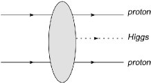
Figure 1: Central Exclusive Production of a Higgs boson.

Detection of both protons by detectors located 420m from the IP at ATLAS/CMS has the virtue that central systems with masses up to 200 GeV can be observed with an event-by-event precision of around 2 to 3 GeV, and adding also 220m detectors extends the reach to much higher masses. The clean environment of CEP generally makes for reduced backgrounds (even in the presence of significant amounts of pile-up) and that is often aided by the fact that the centrally produced system is predominantly in a $J_{z}=0$, C-even, P-even state. Of course having such a spin-parity filter also provides an excellent handle on the nature of any new physics. For very little extra cost, forward detectors promise to significantly enhance the physics potential of the LHC.

That said, CEP is not without its challenges. The theory is difficult, triggering can be tricky, signal rates for new physics are often low, new detectors need building and installing, and pile-up needs to be brought under control. With the arrival of data on CEP from CDF at the Tevatron, confidence is building in the theoretical modelling and extensive studies have demonstrated that all of the other challenges can be met, e.g. see [1].

Figure 2: The relevant lowest order Feynman diagram for $qq\to q+H+q$.

Without further ado, let us very quickly review the Durham model for CEP, more details can be found in [2, 3]. The calculation starts from the easier to compute parton level process $qq\to q+H+q$ shown in Fig. 2. The Higgs is produced via a top quark loop and a minimum of two gluons need to be exchanged in order that no colour be transferred between the incoming and outgoing quarks. The real part of the amplitude is small and the imaginary part can be determined by considering only the cut diagram in Fig. 2. The calculation of the amplitude is straightforward:

$${\mathrm{Im}}A^{ik}_{jl} = \int d(PS)_{2}\;\delta((q_{1}-Q)^{2})\delta((q_{2}+Q)^{2})$$ (1)

$$\frac{2gq_{1}^{\alpha}\;2gq_{2\alpha}}{Q^{2}}\;\frac{2gq_{1}^{\mu}}{k_{1}^{2}}\;\frac{2gq_{2}^{\nu}}{k_{2}^{2}}\;V^{ab}_{\mu\nu}\;\tau^{c}_{im}\tau^{c}_{jn}\tau^{a}_{mk}\tau^{b}_{nl}~{}.$$

We write $Q=\alpha q_{1}+\beta q_{2}+Q_{T}$. The delta functions fix the cut quark lines to be on-shell, which means that $\alpha\approx-\beta\approx\mathbf{Q}_{T}^{2}/s\ll 1$ and $Q^{2}\approx Q_{T}^{2}\equiv-\mathbf{Q}_{T}^{2}$. As always, we neglect terms that are energy suppressed such as the product $\alpha\beta$. In the Standard Model, the Higgs production vertex is

$$V^{ab}_{\mu\nu}=\delta^{ab}\left(g_{\mu\nu}-\frac{k_{2\mu}k_{1\nu}}{k_{1}\cdot k_{2}}\right)V~{},$$ (2)

where $V=m_{H}^{2}\alpha_{s}/(4\pi v)F(m_{H}^{2}/m_{t}^{2})$ and $F\approx 2/3$ provided the Higgs is not too heavy. The Durham group also include a NLO K-factor correction to this vertex.

We can compute the contraction $q_{1}^{\mu}V^{ab}_{\mu\nu}q_{2}^{\nu}$ either directly or by utilising gauge invariance, which requires that $k_{1}^{\mu}V^{ab}_{\mu\nu}=k_{2}^{\nu}V^{ab}_{\mu\nu}=0$. Writing $k_{i}=x_{i}q_{i}+k_{iT}$ yields

$$q_{1}^{\mu}V^{ab}_{\mu\nu}q_{2}^{\nu}\approx\frac{k_{1T}^{\mu}}{x_{1}}\frac{k_{2T}^{\nu}}{x_{2}}V^{ab}_{\mu\nu}\approx\frac{s}{m_{H}^{2}}k_{1T}^{\mu}k_{2T}^{\nu}V^{ab}_{\mu\nu}$$ (3)

since $2k_{1}\cdot k_{2}\approx x_{1}x_{2}s\approx m_{H}^{2}$. Note that it is as if the gluons which fuse to produce the Higgs are transversely polarized, $\epsilon_{i}\sim k_{iT}$. Moreover, in the limiting case that the outgoing quarks carry no transverse momentum $Q_{T}=-k_{1T}=k_{2T}$ and so $\epsilon_{1}=-\epsilon_{2}$. This is an important result; it generalizes to the statement that the centrally produced system should have a vanishing $z$-component of angular momentum in the limit that the protons scatter through zero angle (i.e. $~{}q_{iT}^{\prime 2}\ll Q_{T}^{2}$). Since we are interested in very small angle scattering this selection rule is effective. One immediate consequence is that the Higgs decay to $b$-quarks may now be viable. This is because, for massless quarks, the lowest order $q\bar{q}$ background vanishes identically (it does not vanish at NLO). The leading order $b\bar{b}$ background is therefore suppressed by a factor $\sim m_{b}^{2}/m_{H}^{2}$.

Returning to the task in hand, we can write ($y$ is the rapidity of the Higgs)

$$\frac{d\sigma}{d^{2}\mathbf{q}_{1T}^{\prime}d^{2}\mathbf{q}_{2T}^{\prime}dy} \approx \left(\frac{N_{c}^{2}-1}{N_{c}^{2}}\right)^{2}\frac{\alpha_{s}^{6}}{(2\pi)^{5}}\frac{G_{F}}{\surd{2}}$$ (4)

$$\times\left[\int\frac{d^{2}\mathbf{Q}_{T}}{2\pi}\frac{\mathbf{k}_{1T}\cdot\mathbf{k}_{2T}}{\mathbf{Q}_{T}^{2}\mathbf{k}_{1T}^{2}\mathbf{k}_{2T}^{2}}\frac{2}{3}\right]^{2}~{}.$$

We are mainly interested in the forward scattering limit whence

$$\frac{\mathbf{k}_{1T}\cdot\mathbf{k}_{2T}}{\mathbf{Q}_{T}^{2}\mathbf{k}_{1T}^{2}\mathbf{k}_{2T}^{2}}\approx-\frac{1}{\mathbf{Q}_{T}^{4}}.$$

As it stands, the integral over $Q_{T}$ diverges. Let us not worry about that for now and instead turn our attention to how to convert this parton level cross-section into the hadron level cross-section we need.

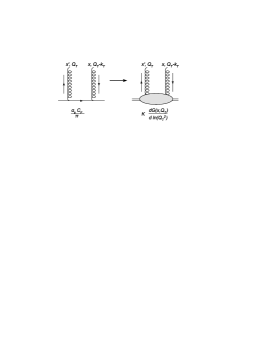
Figure 3: The recipe for replacing the quark line (left) by a proton line (right).

What we really want is the hadronic matrix element which represents the coupling of two gluons into a proton, and this is really an off-diagonal parton distribution function. At present we don’t have much knowledge of these distributions, however we do know the diagonal gluon distribution function. Fig. 3 illustrates the Durham prescription for coupling the two gluons into a proton rather than a quark. The factor $K$ would equal unity if $x^{\prime}=x$ and $k_{T}=0$, which is the diagonal limit. That we should, in the amplitude, replace a factor of $\alpha_{s}C_{F}/\pi$ by $\partial G(x,Q_{T})/\partial\ln Q_{T}^{2}$ can be easily derived starting from the DGLAP equation for evolution off an initial quark distribution given by $q(x)=\delta(1-x)$. The Durham approach makes use of a result derived in [4] which states that in the case $x^{\prime}\ll x$ and $k_{T}^{2}\ll Q_{T}^{2}$ the off-diagonality can be approximated by a multiplicative factor, $K$. Assuming a Gaussian form factor suppression for the $k_{T}$-dependence they estimate that

$$K\approx e^{-bk_{T}^{2}/2}\frac{2^{2\lambda+3}}{\surd{\pi}}\frac{\Gamma(\lambda+5/2)}{\Gamma(\lambda+4)}$$ (5)

and this result is obtained assuming a simple power-law behaviour of the gluon density, i.e. $G(x,Q)\sim x^{-\lambda}$. For the production of a 120 GeV Higgs boson at the LHC, $K\sim 1.2\times e^{-bk_{T}^{2}/2}$. In the cross-section, the off-diagonality therefore provides an enhancement of $(1.2)^{4}\approx 2$. Clearly the current lack of knowledge of the off-diagonal gluon is one source of uncertainty in the calculation. The slope parameter $b$ is fixed by assuming the same $k_{T}$-dependence as for diffractive $J/\psi$ production, i.e. $b\approx 4$ GeV^-2.

Thus, after integrating over the transverse momenta of the scattered protons we have

$$\frac{d\sigma}{dy} \approx \frac{1}{256\pi b^{2}}\frac{\alpha_{s}G_{F}\surd{2}}{9}$$ (6)

$$\times\left[\int\frac{d^{2}\mathbf{Q}_{T}}{\mathbf{Q}_{T}^{4}}\;f(x_{1},Q_{T})f(x_{2},Q_{T})\right]^{2}$$

where $f(x,Q)\equiv\partial G(x,Q)/\partial\ln Q^{2}$ and we have neglected the exchanged transverse momentum in the integrand.

Now it is time to worry about the fact that our integral diverges in the infra-red. Fortunately I have missed some crucial physics. The lowest order diagram is not enough, virtual graphs possess logarithms in the ratio $Q_{T}/m_{H}$ which are very important as $Q_{T}\to 0$; these logarithms need to be summed to all orders. This is Sudakov physics: thinking in terms of real emissions we must be sure to forbid real emissions into the final state. Let’s worry about real gluon emission off the two gluons which fuse to make the Higgs. The emission probability for a single gluon is (assuming for the moment a fixed coupling $\alpha_{s}$)

$$\frac{C_{A}\alpha_{s}}{\pi}\int_{Q_{T}^{2}}^{m_{H}^{2}/4}\frac{dp_{T}^{2}}{p_{T}^{2}}\int_{p_{T}}^{m_{H}/2}\frac{dE}{E}$$ (7)

$$=\frac{C_{A}\alpha_{s}}{4\pi}\ln^{2}\left(\frac{m_{H}^{2}}{Q_{T}^{2}}\right).$$

The integration limits are kinematic except for the lower limit on the $p_{T}$ integral. The fact that emissions below $Q_{T}$ are forbidden arises because the gluon not involved in producing the Higgs completely screens the colour charge of the fusing gluons if the wavelength of the emitted radiation is long enough, i.e. if $p_{T}<Q_{T}$. Now we see how this helps us solve our infra-red problem: as $Q_{T}\to 0$ so the screening gluon fails to screen and real emission off the fusing gluons cannot be suppressed. To see this argument through to its conclusion we realise that multiple real emissions exponentiate and so we can write the non-emission probability as

$$e^{-S}=\exp\left(-\frac{C_{A}\alpha_{s}}{\pi}\int_{Q_{T}^{2}}^{m_{H}^{2}/4}\frac{dp_{T}^{2}}{p_{T}^{2}}\int_{p_{T}}^{m_{H}/2}\frac{dE}{E}\right).$$ (8)

As $Q_{T}\to 0$ the exponent diverges and the non-emission probability vanishes faster than any power of $Q_{T}$. In this way our integral over $Q_{T}$ becomes

$$\int\frac{dQ_{T}^{2}}{Q_{T}^{4}}f(x_{1},Q_{T})f(x_{2},Q_{T})\;e^{-S}~{},$$ (9)

which is finite.

Now Eq. (8) is correct only so far as the leading double logarithms. It is of considerable practical importance to correctly include also the single logarithms. To do this we must re-instate the running of $\alpha_{s}$ and allow for the possibility that quarks can be emitted. Including this physics means we ought to use

$$e^{-S} = \exp\left(-\int_{Q_{T}^{2}}^{m_{H}^{2}/4}\frac{dp_{T}^{2}}{p_{T}^{2}}\frac{\alpha_{s}(p_{T}^{2})}{2\pi}\right.$$

$$\left.\times\int^{1-\Delta}_{0}dz\;[zP_{gg}(z)+\sum_{q}P_{qg}(z)]\right)$$

where $\Delta=2p_{T}/m_{H}$, and $P_{gg}(z)$ and $P_{qg}(z)$ are the leading order DGLAP splitting functions. To correctly sum all single logarithms requires some care in that what we want is the distribution of gluons in $Q_{T}$ with no emission up to $m_{H}$, and this is in fact [5]

$$\tilde{f}(x,Q_{T})=\frac{\partial}{\partial\ln Q_{T}^{2}}\left(e^{-S/2}\;G(x,Q_{T})\right).$$

The integral over $Q_{T}$ is therefore

$$\int\frac{dQ_{T}^{2}}{Q_{T}^{4}}\tilde{f}(x_{1},Q_{T})\tilde{f}(x_{2},Q_{T})~{},$$

which reduces to Eq. (9) in the double logarithmic approximation.

Before we can go ahead and compute the cross-section we need to introduce the idea of gap survival. The Sudakov factor has allowed us to ensure that the exclusive nature of the final state is not spoilt by perturbative emission off the hard process. What about non-perturbative particle production? The protons can in principle interact quite apart from the perturbative process discussed hitherto and this interaction could well lead to the production of additional particles. We need to account for the probability that such emission does not occur. Provided the hard process leading to the production of the Higgs occurs on a short enough timescale, we might suppose that the physics which generates extra particle production factorizes and that its effect can be accounted for via an overall factor multiplying the cross-section we have just calculated. This is the “gap survival factor”. The gap survival, $S^{2}$, is thus defined by

$$d\sigma(p+H+p|\mathrm{no~{}soft~{}emission})=d\sigma(p+H+p)\times S^{2}$$

where $d\sigma(p+H+p)$ is the differential cross-section computed above. The task is to estimate $S^{2}$. Clearly this is not straightforward since we cannot utilize QCD perturbation theory. That said, data on a variety of processes observed at HERA, the Tevatron and the LHC can help us improve our understanding of “gap survival” and to date the HERA and Tevatron data do support the idea of gap survival. For the purposes of this talk we will presume to know the gap survival factor and that $S^{2}=3\%$ for CEP at the LHC, e.g. see [6] for an overview.

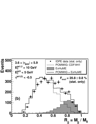
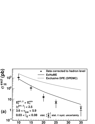
Figure 4: CDF data on CEP dijet production. Figures from [7].

Recently, the CDF collaboration has observed a $6\sigma$ excess of CEP of dijets at the Tevatron [7]. The agreement with the theory (as implemented in the ExHuME monte carlo generator [8]) is very good, as illustrated in Fig. 4. CDF also sees a suppression of quark jets in the exclusive region (high $R_{jj}$), in accord with theoretical expectations.

2 Higgs: SM and MSSM

Fig. 5 shows how the cross-section for producing a SM Higgs boson varies with Higgs mass (and for different gluon distribution functions). The cross-section is small and leads to low production rates. That said, a SM Higgs with mass above 120 GeV should be observable in the $WW^{*}$ channel with 300 fb^-1 of data (which is around 3 years of high luminosity running) [1, 9]. The gold-plated fully leptonic channel has very low backgrounds and has the advantage that one can still use the forward detectors to measure the mass.

The $b\bar{b}$ channel is much more challenging. Triggering in this case would certainly benefit from having 220m detectors in place but even then one relies on optimistic scenarios for the production cross-section, detector acceptance and trigger efficiency. Nevertheless, it ought to be born in mind that CEP may be the only way to explore this channel at the LHC.

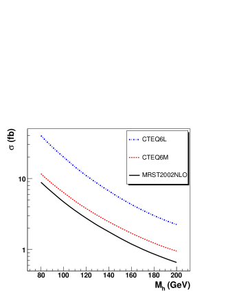
Figure 5: CEP cross-section for Standard Model Higgs producton. Figure from [1].

In contrast, the $b\bar{b}$ channel becomes much more exciting in certain MSSM scenarios. Rates are strongly enhanced at large $\tan\beta$ and small $m_{A}$, and the potential to measure the $hbb$ Yukawa coupling is a strong selling point for CEP and a pre-requisite to determining any Higgs-boson coupling at the LHC (rather than just ratios of couplings). Fig. 6 shows the region of parameter space in which one could observe $h\to b\bar{b}$ using CEP [10] with different amounts of integrated luminosity. A similar pair of plots can be produced for $H\to b\bar{b}$, see [10]. Fig. 7 shows the result of an in-depth analysis of one particular point in the $m_{A}-\tan\beta$ plane ($\tan\beta=40$ and $m_{A}=120$ GeV) [13]. The details of the two analyses can be found in [1, 10, 13] but the key point is that they are in general agreement

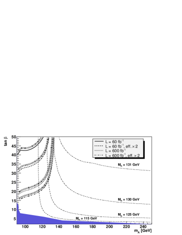
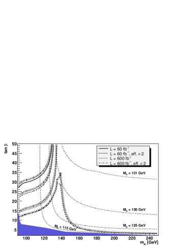
Figure 6: $5\sigma$ discovery contours (upper plot) and contours of $3\sigma$ statistical significance (lower plot) for the $h\to b\bar{b}$ channel in CEP in the $M_{A}$ - tan$\beta$ plane of the MSSM within the $M_{h,{\mathrm{max}}}$ benchmark scenario for different luminosity scenarios as described in the text [10]. The values of the mass of the light CP-even Higgs boson, $M_{h}$, are indicated by contour lines. No pile-up background assumed. The dark shaded (blue) region corresponds to the parameter region that is excluded by the LEP Higgs boson searches [11, 12]. Figure from [1].

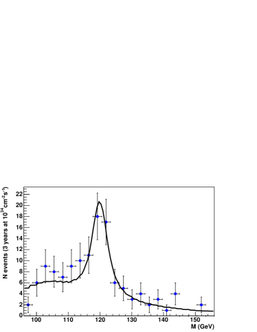
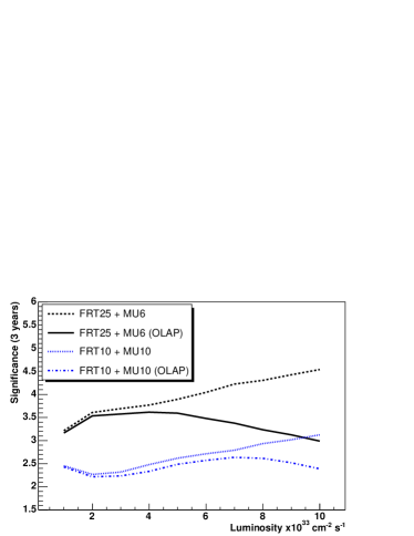
Figure 7: Upper: Typical mass fit for the 120 GeV MSSM $h\rightarrow b\bar{b}$ for 3 years of data taking at $10^{34}~{}$cm${}^{-2}~{}$s^-1 after removing the overlap background contribution completely with improved timing detectors. The significance is $5\sigma$ for these data. Lower: Significance of the measurement of the 120 GeV MSSM Higgs boson versus luminosity, for two different combinations of muon (MU6, MU10) and fixed-jet-rate (FRT25, FRT10) triggers and with an improved (baseline) FP420 timing design (OLAP labels). Figure from [1].

The curves in Fig. 7 correspond to different trigger scenarios. They also indicate the influence of pile-up and, in particular, the overlap background (OLAP), in which the signal is faked by a coincidence of events, one that produces the central system (which fakes the Higgs decay) and one or more diffractive events that are able to produce protons in the forward detectors, e.g. a three-fold co-incidence of two single diffractive events with a $pp\to b\bar{b}X$ event. Use of fast-timing detectors allows a significant reduction in the OLAP background, as the primary vertex can be pinpointed to high accuracy. Improvements in the fast-timing could potentially eliminate the OLAP background completely and allow a $5\sigma$ discovery with 3 years of high luminosity data taking (the mass peak is illustrated in the upper plot in Fig. 7).

3 Higgs: NMSSM

To conclude, I would like to take a slightly more in-depth look at the possibilities for CEP of NMSSM Higgs bosons. More details can be found in [14]. The NMSSM is an extension of the MSSM that solves the $\mu$-problem, and also the little hierarchy problem, by adding a gauge-singlet superfield $\hat{S}$ to the MSSM such that the $\mu$ term is now dynamical in origin, arising when the scalar member of $\hat{S}$ aquires a vev. The $\mu$ problem is solved since $\mu$ is no longer fundamental and therefore no longer naturally of order the GUT scale (as is the case if it is the only dimensionful parameter in the superpotential). The little heirarchy problem is also solved because a lighter Higgs is allowed, thereby taking the pressure off the stop mass. More specifically, the lightest scalar Higgs can decay predominantly to two pseudo-scalar Higgses and the branching ratio to $b$-quarks is correspondingly suppressed, thereby evading the 114 GeV bound from LEP. Having a lighter Higgs means that the stop mass does not need to be so large, and that is preferred given the value of $M_{Z}$.

The Higgs sector of the NMSSM extends that of the MSSM by adding an extra pseudo-scalar Higgs and an extra scalar Higgs: crucially $\hat{S}$ is a gauge singlet and hence $h\to aa$ can dominate with a light $a$ (i.e. below the threshold for $a\to b\bar{b}$).

Figure 8: CEP of an NMSSM Higgs.

Freed of the heavy stop, it is most natural to have a light Higgs with a reducing branching ratio to $b$-quarks, as illustrated in Fig. 9. $F$ and $G$ are measures of fine-tuning, so the points in this scatter plot are supposed to represent most natural scenarios in the NMSSM. Our attention will focus on one such point, with $m_{h}=93$ GeV and $m_{a}=9.7$ GeV with BR$(h\to aa)=92\%$ and BR$(a\to\tau\tau)=81\%$ [15]. The lightness of the pseudo-scalar $a$ means that the $h$ decays predominantly to four taus. Should such a decay mode be dominant at the LHC, standard search strategies would fail and, as we shall see, CEP (as illustrated in Fig. 8) could provide the discovery channel. This “natural” scenario of the NMSSM has two additional bonus features that one might draw attention to: 1. a light Higgs is preferred by the precision electroweak data (recall the best fit value is somewhat below 100 GeV); 2. a 100 GeV Higgs with a reduced (10%) branching ratio to $b$-quarks naturally accommodates the existing $2.3\sigma$ LEP excess in $e^{+}e^{-}\to Zb\bar{b}$ [16, 17].

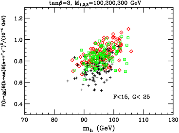
Figure 9: $\Gamma_{\mathrm{eff}}$ in units of $10^{-4}\mathrm{GeV}^{2}$ versus $m_{h}$ for $\mathrm{tan}\beta=3$. Point coding: (red) diamonds = $2m_{\tau}<m_{a}<7.5\mathrm{GeV}$; (green) squares = $7.5\mathrm{GeV}\leq m_{a}<8.8\mathrm{GeV}$; (black) pluses = $8.8\mathrm{GeV}\leq m_{a}<2m_{b}$. Figure from [14].

To detect the four-tau decay of an NMSSM Higgs using CEP, we need first to trigger the event and to that end demand that at least one of the taus decays to produce a sufficiently high $p_{T}$ muon. The muon then defines a vertex which can be used, in conjunction with the (picosecond) fast timing of the 420m detectors, to reject pile-up related backgrounds. The detailed analysis is outlined in [14], here we shall just highlight the key features. Table 1 shows how the signal (CEP) and backgrounds (DPE, OLAP and QED) are affected by the cuts imposed. The top line of the table is the cross-section after imposing that there be at least one muon with $p_{T}>6$ GeV, which is the nominal minimum value to trigger at level 1 in ATLAS and the condition that both protons be detected in the 420m detectors. There is also a loose cut on the invariant mass of the central system. Of the remaining cuts, I would like to single out the “$N_{\mathrm{ch}}=4$ or 6” cut.

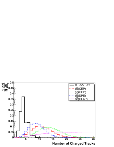
Figure 10: The expected number of charged tracks reconstructed by the ATLAS inner detector with $p_{T}>6$ GeV and $|\eta|<2.5$.

The charged track ($N_{\mathrm{ch}}$) cut is noteworthy because it can be implemented at the highest LHC luminosities: we cut on exactly 4 or 6 charged tracks that point back to the vertex defined by the muon. Pile-up events do add extra tracks (to both the signal and background), but they do not often coincide with the primary vertex (i.e. within a 2.5 mm window) and do not spoil the effectiveness of this cut. The number of charged tracks in signal and background events is illustrated in Fig. 10. The ability to make such hard cuts on charged tracks could be of a much wider utility than this analysis (e.g. in defining a jet veto in Higgs plus two jets production). The four or six track event is then analysed in terms of its topology and the topology cut exploits the fact that the charged tracks originate from four taus in the signal, which themselves originate from two heavily boosted pseudo-scalars. To avoid the effects of pile-up, the analysis is heavily track-based with almost no reliance on the calorimeter.

Accurate measurement of the proton energies allows one to constrain the kinematics of the central system (in particular its invariant mass and mean rapidity are known). We can also extract the masses of the $h$ and the $a$ on an event-by-event basis. The mass of the $h$ is straightforward of course (it is measured directly by the forward detectors) and a precision below 1 GeV can be obtained with just a handful of events. The measurement of the pseudo-scalar mass is more interesting and potentially very important. The proton measurements fix $p_{z}$ and $p_{x,y}\approx 0$ for the central system. In addition, the tau pairs are highly boosted, which means they are collinear with their parent pseudo-scalars. That means that the four-momentum of each pseudo-scalar is approximately proportional to the observed (track) four-momentum. The two unknown constants of proportionality (i.e. the missing energy fractions) are overconstrained, since we have three equations from the proton detectors. The result is that we can solve for the pseudo-scalar masses, with four measurements per event. Fig. 11 shows a typical distribution of $a$ masses based on 180 fb^-1 of data collected at $3\times 10^{33}$ cm^-2s^-1.

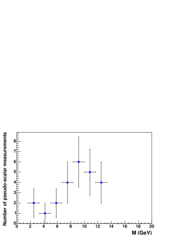
Figure 11: A typical $a$ mass measurement.

Table 1: The table of cross-sections for the signal and backgrounds. All cross-sections are in femtobarns. The overlap (OLAP) background is computed at a luminosity of $10^{34}$ cm^-2 s^-1.

	CEP			DPE	OLAP	QED
Cut	$H$	$b\bar{b}$	$gg$	$b\bar{b}$	$b\bar{b}$	$4\tau$	$2\tau$ $2l$
$p_{T0}^{\mu}$, $\xi_{1}$, $\xi_{2}$, $M$	0.442	25.14	1.51$\times 10^{3}$	1.29$\times 10^{3}$	1.74$\times 10^{6}$	0.014	0.467
$N_{\mathrm{ch}}=$ 4 or 6	0.226	1.59	28.84	1.58$\times 10^{2}$	1.44$\times 10^{4}$	0.003	0.056
$Q_{h}=0$	0.198	0.207	3.77	18.69	1.29$\times 10^{3}$	5$\times 10^{-4}$	0.010
Topology	0.143	0.036	0.432	0.209	1.84	-	$<$0.001
$p_{T}^{\mu}$, isolation	0.083	0.001	0.008	0.003	0.082	-	-
$p_{T}^{1,\not{\mu}}$	0.071	5$\times$10-4	0.004	0.002	0.007	-	-
$m_{a}>2m_{\tau}$	0.066	2$\times$10-4	0.001	0.001	0.005	-	-

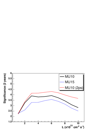
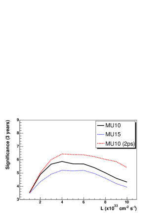
Figure 12: Upper: The significance for three years of data acquisition at each luminosity. Lower: Same as (a) but with twice the data.

In Table 2 I show the bottom line numbers for three different trigger scenarios and three different instantaneous luminosities. The key point is that, although we can expect only a handful of signal events, the background is under control. Remember, we need only a few events in order to extract the masses of both the $a$ and the $h$. The statistical significance of any discovery is estimated in Fig. 12. The lower plot might pertain if the signal rate were doubled (recall the theoretical uncertainty permits it) or if data from ATLAS and CMS were combined or if other leptonic triggers are used [1].

4 Concluding remarks

Central exclusive production is a very attractive prospect for the LHC. A very broad programme of physics can be pursued for very little additional expenditure. Measurements from CDF at the Tevatron are very encouraging and support the validity of the theoretical calculations: the theory is probably not too far off the mark. Moreoever, one of the highlights of the past couple of years has been the demonstration that high luminosity backgrounds can be brought under control. This talk has focussed only upon Higgs physics and has placed particular emphasis on the possibility that CEP could be the only way one could observe at the LHC a Higgs boson that decays predominantly to four taus: something that could be fairly generic feature of SUSY models with an enlarged Higgs sector (such as the NMSSM).

Table 2: Expected number of signal (S) and background (B) events for the three trigger scenarios assuming that the data are collected at a fixed instantaneous luminosity over a three year period. We assume the integrated luminosity acquired each year is 10 fb^-1, 50 fb^-1 and 100 fb^-1 at an instantaneous luminosity of 1$\times 10^{33}$ cm^-2 s^-1 (row 1), 5$\times 10^{33}$ cm^-2 s^-1 (row 2) and 10 $\times 10^{33}$ cm^-2 s^-1 (row 3).

L	MU10		MU15		MU10 (2 ps)
	S	B	S	B	S	B
$1$	1.3	0.02	1.0	0.01	1.3	0.02
$5$	3.7	0.14	2.9	0.08	3.7	0.07
$10$	3.3	0.36	2.5	0.20	3.3	0.11

References

- [1] M. G. Albrow et al. [FP420 R&D Collaboration], “The FP420 R&D Project: Higgs and New Physics with forward protons at the LHC,” arXiv:0806.0302 [hep-ex].
- [2] V. A. Khoze, A. D. Martin and M. G. Ryskin, Eur. Phys. J. C 23 (2002) 311 [arXiv:hep-ph/0111078].
- [3] J. R. Forshaw, “Diffractive Higgs production: Theory,” arXiv:hep-ph/0508274.
- [4] A. G. Shuvaev, K. J. Golec-Biernat, A. D. Martin and M. G. Ryskin, Phys. Rev. D 60 (1999) 014015 [arXiv:hep-ph/9902410].
- [5] A. D. Martin and M. G. Ryskin, Phys. Rev. D 64 (2001) 094017 [arXiv:hep-ph/0107149].
- [6] A. D. Martin, V. A. Khoze and M. G. Ryskin, “Rapidity gap survival probability and total cross sections,” arXiv:0810.3560 [hep-ph].
- [7] T. Aaltonen et al. [CDF Collaboration], Phys. Rev. D 77, 052004 (2008) [arXiv:0712.0604 [hep-ex]].
- [8] J. Monk and A. Pilkington, Comput. Phys. Commun. 175 (2006) 232 [arXiv:hep-ph/0502077].
- [9] B. E. Cox et al., Eur. Phys. J. C 45 (2006) 401 [arXiv:hep-ph/0505240].
- [10] S. Heinemeyer, V. A. Khoze, M. G. Ryskin, W. J. Stirling, M. Tasevsky and G. Weiglein, Eur. Phys. J. C 53 (2008) 231 [arXiv:0708.3052 [hep-ph]].
- [11] R. Barate et al. [LEP Working Group for Higgs boson searches], Phys. Lett. B 565 (2003) 61 [arXiv:hep-ex/0306033].
- [12] S. Schael et al. [ALEPH Collaboration], Eur. Phys. J. C 47 (2006) 547 [arXiv:hep-ex/0602042].
- [13] B. E. Cox, F. K. Loebinger and A. D. Pilkington, JHEP 0710 (2007) 090 [arXiv:0709.3035 [hep-ph]].
- [14] J. R. Forshaw, J. F. Gunion, L. Hodgkinson, A. Papaefstathiou and A. D. Pilkington, JHEP 0804 (2008) 090 [arXiv:0712.3510 [hep-ph]].
- [15] U. Ellwanger and C. Hugonie, Comput. Phys. Commun. 175 (2006) 290 [arXiv:hep-ph/0508022].
- [16] R. Dermisek and J. F. Gunion, Phys. Rev. Lett. 95 (2005) 041801 [arXiv:hep-ph/0502105].
- [17] R. Dermisek and J. F. Gunion, Phys. Rev. D 73 (2006) 111701 [arXiv:hep-ph/0510322].