CERN-PH-TH/2008-252

Stochastic backgrounds of relic gravitons:

a theoretical appraisal
Massimo Giovannini
Department of Physics, Theory Division, CERN, 1211 Geneva 23, Switzerland
INFN, Section of Milan-Bicocca, 20126 Milan, Italy

Stochastic backgrounds or relic gravitons, if ever detected, will constitute a prima facie evidence of physical processes taking place during the earliest stages of the evolution of the plasma. The essentials of the stochastic backgrounds of relic gravitons are hereby introduced and reviewed. The pivotal observables customarily employed to infer the properties of the relic gravitons are discussed both in the framework of the $\Lambda$CDM paradigm as well as in neighboring contexts. The complementarity between experiments measuring the polarization of the Cosmic Microwave Background (such as, for instance, WMAP, Capmap, Quad, Cbi, just to mention a few) and wide band interferometers (e.g. Virgo, Ligo, Geo, Tama) is emphasized. While the analysis of the microwave sky strongly constrains the low-frequency tail of the relic graviton spectrum, wide-band detectors are sensitive to much higher frequencies where the spectral energy density depends chiefly upon the (poorly known) rate of post-inflationary expansion.

1 The spectrum of the relic gravitons

1.1 The frequencies and wavelengths of relic gravitons

Terrestrial and satellite observations, scrutinizing the properties of the electromagnetic spectrum, are unable to test directly the evolution of the background geometry prior to photon decoupling. The redshift probed by Cosmic Microwave Background (CMB in what follows) observations is of the order of $z_{\mathrm{dec}}\simeq 1087$ and it roughly corresponds to the peak of the visibility function, i.e. when most of the CMB photons last scattered free electrons (and protons). After decoupling the ionization fraction drops; the photons follow null geodesics whose slight inhomogeneities can be directly connected with the fluctuations of the spatial curvature present before matter-radiation decoupling.

The temperature of CMB photons is, today, of the order of $2.725$ K. The same temperature at photon decoupling must have been of the order of about $2962$ K, i.e. $0.25$ eV. The CMB temperature increases linearly with the redshift: this fact may be tested empirically by observing at high redshifts clouds of chemical compounds (like CN) whose excited levels may be populated thanks to the higher value of the CMB temperature [1, 2].

The initial conditions for the processes leading to formation of CMB anisotropies are set well before matter radiation equality and right after neutrino decoupling (taking place for temperatures of the order of the MeV) whose associated redshift is around $10^{10}$. The present knowledge of particle interactions up to energy scales of the order of $200$ GeV certainly provides important (but still indirect) clues on the composition of the plasma.

If ever detected, relic gravitons might provide direct informations on the evolution of the Hubble rate for much higher redshifts. In a rudimentary realization of the $\Lambda$CDM paradigm, the inflationary phase can be modeled in terms of the expanding branch of de-Sitter space. Assuming that, right after inflation, the Universe evolves adiabatically and is dominated by radiation, the redshift associated with the end of inflation can be approximately computed as

$$z+1\simeq 3\times 10^{28}\,\biggl{(}\frac{T_{\gamma 0}}{2.725\,\mathrm{K}}\biggr{)}^{-1}\biggl{(}\frac{H}{10^{-5}\,M_{\mathrm{P}}}\biggr{)}^{1/2}\,\biggl{(}\frac{g_{\rho}}{106.75}\biggr{)}^{-1/4},$$ (1.1)

where $g_{\rho}$ denotes the weighted number of relativistic degrees of freedom at the onset of the radiation dominated evolution and $106.75$ corresponds to the value of the standard model of particle interactions. In Eq. (1.1) it has been also assumed, quite generally, that $H\simeq 10^{-5}\,M_{\mathrm{P}}$ as implied by the CMB observations. For more accurate estimates the quasi-de Sitter nature of the inflationary expansion must be taken into account. In the $\Lambda$CDM paradigm, the basic mechanism responsible for the production of relic gravitons is the parametric excitation of the (tensor) modes of the background geometry and it is controlled by the rate of variation of space-time curvature.

In the present article the $\Lambda$CDM paradigm will always be assumed as a starting point for any supplementary considerations. The reasons for this choice are also practical since the experimental results must always be stated and presented in terms of a given reference model. Having said this, most of the considerations presented here can also be translated (with the appropriate computational effort) to different models.

Given a specific scenario for the evolution of the Universe (like the $\Lambda$CDM model), the relic graviton spectra can be computed. The amplitude of the relic graviton spectrum over different frequencies depends upon the specific evolution of the Hubble rate. The theoretical error on the amplitude increases with the frequency: it is more uncertain (even within a specified scenario) at high frequencies rather than at small frequencies.

The experimental data, at the moment, do not allow either to rule in or to rule out the presence of a primordial spectrum of relic gravitons compatible with the $\Lambda$CDM scenario. The typical frequency probed by CMB experiments is of the order of $\nu_{\mathrm{p}}=k_{\mathrm{p}}/(2\pi)\simeq 10^{-18}\,\mathrm{Hz}=1\,\mathrm{aHz}$ where $k_{\mathrm{p}}$ is the pivot frequency at which the tensor power spectra are assigned. CMB experiments will presumably set stronger bounds on the putative presence of a tensor background for frequencies ${\mathcal{O}}(\mathrm{aHz})$. This bound will be significant also for higher frequencies only if the whole post-inflationary thermal history is assumed to be known and specified.

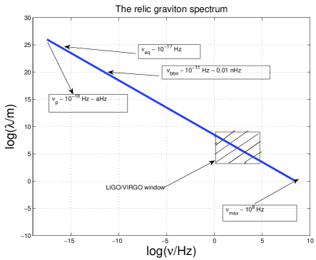
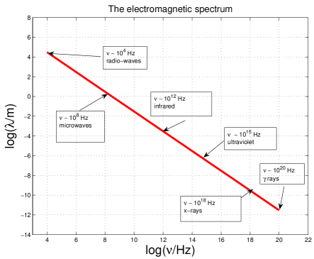
Figure 1: A schematic view of the frequency range of the relic graviton spectrum (plot at the left) and of the electromagnetic spectrum (plot at the right). In both plots the common logarithms of the (comoving) frequency and of the (comoving) wavelengths are reported, respectively, on the horizontal and on the vertical axis.

The typical frequency window of wide-band interferometers (such as Ligo and Virgo) is located between few Hz and $10$ kHz, i.e. roughly speaking, $20$ orders of magnitude larger than the frequency probed by CMB experiments. The frequency range of wide-band interferometers will be conventionally denoted by $\nu_{\mathrm{LV}}$. To compute the relic graviton spectrum over the latter range of frequencies, the evolution of our Universe should be known over a broad range of redshifts. We do have some plausible guesses on the evolution of the plasma from the epoch of neutrino decoupling down to the epoch of photon decoupling. The latter range of redshifts corresponds to an interval of comoving frequencies going from $\nu_{\mathrm{p}}\simeq 10^{-18}$ Hz up to $\nu_{\mathrm{bbn}}\simeq 0.01\,\mathrm{nHz}\sim 10^{-11}\,$ Hz (at most).

In Fig. 1 (plot at the left) the frequency range of the relic graviton spectrum is illustrated, starting from the (comoving) frequency $\nu_{\mathrm{p}}$ whose associated (comoving) wavelength is of the order of of $10^{26}$ m, i.e. roughly comparable with the Hubble radius at the present time. The low-frequency branch of the spectrum can be conventionally defined between $\nu_{\mathrm{p}}$ and $\nu_{\mathrm{bbn}}$. The largest frequency of the relic graviton spectrum (i.e. $\nu_{\mathrm{max}}$) is of the order of $0.1$ GHz in the $\Lambda$CDM scenario. Thus the high-frequency branch of the graviton spectrum can be conventionally defined for $\nu_{\mathrm{bbn}}<\nu<\nu_{\mathrm{max}}$. In summary we can therefore say that

• the range $\nu_{\mathrm{p}}<\nu<\nu_{\mathrm{bbn}}$ will be generically referred to as the low-frequency domain; in this range the spectrum of relic gravitons basically follows from the minimal $\Lambda$CDM paradigm;

• the range $\nu_{\mathrm{bbn}}<\nu<\nu_{\mathrm{max}}$ will be generically referred to as the high-frequency domain; in this range the spectrum of relic gravitons is more uncertain.

The high-frequency branch of the relic graviton spectrum, overlapping with the frequency window of wide-band detectors (see shaded box in the left plot of Fig. 1), is rather sensitive to the thermodynamic history of the plasma after inflation as well as, for instance, to the specific features of the underlying gravity theory at small scales. This is why we said that the theoretical error in the calculation of the relevant observables increases, so to speak, with the frequency.

In Fig. 1 (plot at the right) the electromagnetic spectrum is reported in its salient features. It seems instructive to draw a simple minded parallel between the electromagnetic spectrum and the spectrum of relic gravitons. Consider first the spectrum of relic gravitons (see Fig. 1, plot at the left): between $10^{-18}$ Hz (corresponding to $\nu_{\mathrm{p}}$) and $10$ kHz (corresponding to $\nu_{\mathrm{LV}}$) there are, roughly, 22 decades in frequency. A similar frequency gap (see Fig. 1, plot at the right), if applied to the well known electromagnetic spectrum, would drive us from low-frequency radio waves up to x-rays or $\gamma$-rays. As the physics explored by radio waves is very different from the physics probed by $\gamma$ rays, it can be argued that the informations carried by low and high frequency gravitons originate from two very different physical regimes of the theory. Low frequency gravitons are sensitive to the large scale features of the given cosmological model and of the underlying theory of gravity. High frequency gravitons are sensitive to the small scale features of a given cosmological model and of the underlying theory of gravity.

The interplay between long wavelength gravitons and CMB experiments will be specifically discussed in the subsection 1.2. The main message will be that, according to current CMB experiments, long wavelength gravitons have not been observed yet. The latter occurrence imposes a very important constraint on the low frequency branch of the relic graviton spectrum of the $\Lambda$CDM scenario whose salient predictions will be introduced in subsection 1.3. According to the minimal $\Lambda$CDM paradigm a very peculiar conclusion seems to pop up: the CMB constraints on the low-frequency tail of the graviton spectrum jeopardize the possibility of any detectable signal for frequencies comparable with the window explored by wide band interferometers (see subsection 1.4). The natural question arising at this point is rather simple: is it possible to have a quasi-flat low-frequency branch of the relic graviton spectrum and a sharply increasing spectral energy density at high-frequencies? This kind of signal is typical of a class of completions of the $\Lambda$CDM paradigm which have been recently dubbed T$\Lambda$CDM (for tensor -$\Lambda$CDM). The main predictions of these models will be introduced in subsection 1.5. We shall conclude this introductory section with a discussion of two relevant constraints which should be applied to relic graviton backgrounds in general, i.e. the millisecond pulsar and the big-bang nucleosynthesis constraint (see subsection 1.6).

1.2 Long wavelength gravitons and CMB experiments

The bounds on the backgrounds of relic gravitons stemming from CMB experiments are phrased in terms of $r_{\mathrm{T}}$ which is the ratio between the tensor and the scalar power spectra at the same conventional scale (often called pivot scale). While the use of $r_{\mathrm{T}}$ is practical (see e. g. the 5-year WMAP data [3, 4, 5, 6, 7]), it assumes the $\Lambda$CDM scenario insofar as the curvature perturbations are adiabatic. Within the $\Lambda$CDM model, the tensor and scalar power spectra can be parametrized as

$${\mathcal{P}}_{\mathrm{T}}(k)={\mathcal{A}}_{\mathrm{T}}\biggl{(}\frac{k}{k_{\mathrm{p}}}\biggr{)}^{n_{\mathrm{T}}},\qquad{\mathcal{A}}_{\mathrm{T}}=r_{\mathrm{T}}{\mathcal{A}}_{{\mathcal{R}}},$$ (1.2)

$${\mathcal{P}}_{{\mathcal{R}}}(k)={\mathcal{A}}_{{\mathcal{R}}}\biggl{(}\frac{k}{k_{\mathrm{p}}}\biggr{)}^{n_{\mathrm{s}}-1},\qquad{\mathcal{A}}_{{\mathcal{R}}}=(2.41\pm 0.11)\times 10^{-9},\qquad k_{\mathrm{p}}=0.002\,\,\mathrm{Mpc}^{-1}.$$ (1.3)

where $k_{\mathrm{p}}$ is the pivot wave-number and ${\mathcal{A}}_{{\mathcal{R}}}$ is the amplitude of the power spectrum of curvature perturbations computed at $k_{\mathrm{p}}$; $n_{\mathrm{s}}$ and $n_{\mathrm{T}}$ are, respectively, the scalar and the tensor spectral indices . The value of $k_{\mathrm{p}}$ is conventional and it corresponds to an effective harmonic $\ell_{\mathrm{eff}}\simeq 30$. The figure for ${\mathcal{A}}_{\mathcal{R}}$ quoted in Eq. (1.3) corresponds to the value inferred from the WMAP 5-year data [3, 4, 5, 6, 7] in combination with the minimal $\Lambda$CDM model. In the $\Lambda$CDM model the origin of ${\mathcal{A}}_{{\mathcal{R}}}$ stems from adiabatic curvature perturbations which are present after neutrino decoupling but before matter radiation equality (taking place at a redshift $z_{\mathrm{eq}}=3176_{-150}^{+151}$ according to the WMAP 5-yr data [3, 4, 5]). The dominant component of curvature perturbations is adiabatic meaning that, over large scales, the fluctuations in the specific entropy are vanishing, at least in the minimal version of the model. The adiabatic nature of the fluctuations induces a simple relation between the first acoustic peak of the TT power spectra and the first anticorrelation peak of the TE power spectra [9]: this is, to date, the best evidence that curvature perturbations are, predominantly, adiabatic. It is useful to translate the comoving wave number $k_{\mathrm{p}}$ into a comoving frequency

$$\nu_{\mathrm{p}}=\frac{k_{\mathrm{p}}}{2\pi}=3.092\times 10^{-18}\,\,\mathrm{Hz}\equiv 3.092\,\,\mathrm{aHz},$$ (1.4)

so, as anticipated, $\nu_{\mathrm{p}}$ is of the order of the aHz. The amplitude at the pivot scale is controlled exactly by $r_{\mathrm{T}}$. The combined analysis of the CMB data, of the large-scale (LSS) structure data [13, 14] and of the supernova (SN) data [15, 16] can lead to quantitative upper limits on $r_{\mathrm{T}}$ which are illustrated in Tabs. 1 and 2 as they are emerge from the combined analyses of different data sets.

Data	$r_{\mathrm{T}}$	$n_{\mathrm{s}}$	$\alpha_{\mathrm{S}}$	$\Omega_{\Lambda}$	$\Omega_{\mathrm{M}0}$	$k_{\mathrm{eq}}\mathrm{Mpc}$
WMAP5 alone	$<0.58$	$1.087_{-0.073}^{0.072}$	$-0.050\pm 0.034$	$0.722_{-0.057}^{+0.054}$	$0.278_{-0.054}^{0.057}$	$0.00993$
WMAP5 + Acbar	$<0.54$	$1.083_{-0.062}^{0.063}$	$-0.048\pm 0.027$	$0.719_{-0.047}^{+0.048}$	$0.281_{-0.048}^{0.047}$	$0.01004$
WMAP5+ LSS + SN	$<0.54$	$1.093_{-0.069}^{0.068}$	$-0.055_{-0.028}^{0.027}$	$0.714_{-0.016}^{+0.017}$	$0.286_{-0.017}^{0.016}$	$0.01008$
WMAP5+ CMB data	$<0.64$	$1.127_{-0.071}^{0.075}$	$-0.072_{-0.030}^{+0.031}$	$0.704_{-0.054}^{0.055}$	$0.296_{-0.055}^{0.054}$	$0.01013$

Table 1: The change in determination of the parameters of the tensor background for three different choices of cosmological data sets.

The inferred values of the scalar spectral index (i.e. $n_{\mathrm{s}}$), of the dark energy and dark matter fractions (i.e., respectively, $\Omega_{\Lambda}$ and $\Omega_{\mathrm{M}0}$), and of the typical wavenumber of equality $k_{\mathrm{eq}}$ are reported in the remaining columns. While different analyses can be performed, it is clear, by looking at Tabs. 1 and 2, that the typical upper bounds on $r_{\mathrm{T}}(k_{\mathrm{p}})$ range between, say, $0.2$ and $0.4$. More stringent limits can be obtained by adding supplementary assumptions.

Data	$r_{\mathrm{T}}$	$n_{\mathrm{s}}$	$\alpha_{\mathrm{S}}$	$\Omega_{\Lambda}$	$\Omega_{\mathrm{M}0}$	$k_{\mathrm{eq}}\mathrm{Mpc}$
WMAP5 alone	$<0.43$	$0.986\pm 0.22$	$0$	$0.770_{-0.032}^{+0.033}$	$0.230_{-0.033}^{0.032}$	$0.00936$
WMAP5 + Acbar	$<0.40$	$0.985_{-0.020}^{0.019}$	$0$	$0.767\pm 0.032$	$0.233\pm 0.032$	$0.00944$
WMAP5+ LSS + SN	$<0.20$	$0.968\pm 0.015$	$0$	$0.725\pm 0.015$	$0.275\pm 0.015$	$0.00999$
WMAP5+ CMB data	$<0.36$	$0.979\pm 0.020$	$0$	$0.775\pm 0.032$	$0.225\pm 0.032$	$0.00922$

Table 2: Same as in Tab. 1 but assuming no running in the (scalar) spectral index (i.e. $\alpha_{\mathrm{S}}=0$).

In Tab. 1 the quantity $\alpha_{\mathrm{S}}$ determines the frequency dependence of the scalar spectral index. In the simplest case $\alpha_{\mathrm{S}}=0$ and the spectral index is frequency-independent (i.e. $n_{\mathrm{s}}$ does not run with the frequency). It can also happen, however, that $\alpha_{\mathrm{S}}\neq 0$ which implies an effective frequency dependence of the spectral index. If the inflationary phase is driven by a single scalar degree of freedom (as contemplated in the minimal version of the $\Lambda$CDM scenario) and if the radiation dominance kicks in almost suddenly after inflation, the whole tensor contribution can be solely parametrized in terms of $r_{\mathrm{T}}$. The rationale for the latter statement is that $r_{\mathrm{T}}$ not only determines the tensor amplitude but also, thanks to the algebra obeyed by the slow-roll parameters, the slope of the tensor power spectrum, customarily denoted by $n_{\mathrm{T}}$. To lowest order in the slow-roll expansion, therefore, the tensor spectral index is slightly red and it is related to $r_{\mathrm{T}}$ (and to the slow-roll parameter) as

$$n_{\mathrm{T}}\simeq-\frac{r_{\mathrm{T}}}{8}\simeq-2\epsilon,\qquad\epsilon=-\frac{\dot{H}}{H^{2}},$$ (1.5)

where $\epsilon$ measures the rate of decrease of the Hubble parameter during the inflationary epoch . Within the established set of conventions the scalar spectral index $n_{\mathrm{s}}$ is given by $n_{\mathrm{s}}=(1-6\epsilon+2\overline{\eta})$ and it depends not only upon $\epsilon$ but also upon the second slow-roll parameter $\overline{\eta}=\overline{M}_{\mathrm{P}}^{2}V_{,\varphi\varphi}/V$ (where $V$ is the inflaton potential, $V_{,\varphi\varphi}$ denotes the second derivative of the potential with respect to the inflaton field and $\overline{M}_{\mathrm{P}}=1/\sqrt{8\pi G}$). It is sometimes assumed that also $n_{\mathrm{T}}$ is not constant but it is rather a function of the wavenumber, i.e.

$$n_{\mathrm{T}}(k)=-2\epsilon+\frac{\alpha_{\mathrm{T}}}{2}\ln{(k/k_{\mathrm{p}})},\qquad\alpha_{\mathrm{T}}=\frac{r_{\mathrm{T}}}{8}\biggl{[}(n_{\mathrm{s}}-1)+\frac{r_{\mathrm{T}}}{8}\biggr{]},$$ (1.6)

where $\alpha_{\mathrm{T}}$ now measures the running of the tensor spectral index.

As already mentioned, among the CMB experiments a central role is played by WMAP [3, 4, 5, 6, 7] (see also [8, 9, 10] for first year data release and [11, 12] for the third year data release. In connection with [3, 4, 5, 6, 7], the WMAP 5-year data have been also combined with observations of the Acbar experiment [17, 18, 19, 20] . The TT, TE and, partially EE angular power spectra have been measured by the WMAP experiment. Other (i.e. non space-borne) experiments are now measuring polarization observables, in particular there are

• the Dasi (degree angular scale interferometer) experiment [21, 22, 23] operating at south pole ;

• the Capmap (cosmic anisotropy polarization mapper) experiment [24, 25] ;

• the Cbi (cosmic background imager) experiment [26, 27];

• the Quad experiment [28, 29, 30];

as well as various other experiments at different stages of development . In the near future the Planck explorer satellite [31] might be able to set more direct limits on $r_{\mathrm{T}}$ by measuring (hopefully) the BB angular power spectra.

1.3 The relic graviton spectrum in the $\Lambda$CDM model

Having defined the frequency range of the spectrum of relic gravitons, it is now appropriate to illustrate the possible signal which is expected within the $\Lambda$CDM scenario.

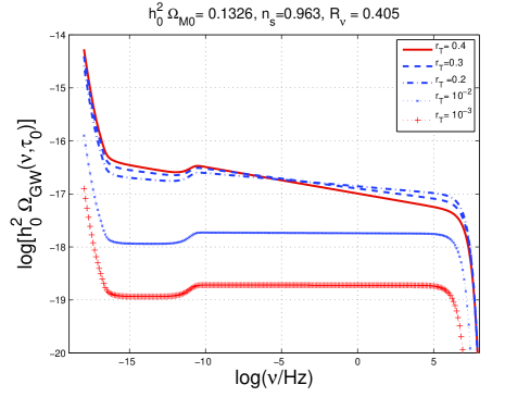
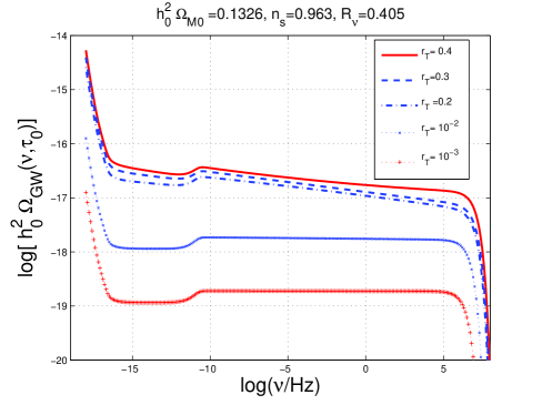
Figure 2: The spectral energy density of the relic gravitons is illustrated the context of the $\Lambda$CDM scenario and for different values of $r_{\mathrm{T}}$ (see Eqs. (1.2)–(1.3)). In the plot at the right the tensor spectral index $n_{\mathrm{T}}$ does depend upon the frequency ($\alpha_{\mathrm{T}}$ follows from Eq. (1.6) with the $\Lambda$CDM choice of parameters). The plot at the left corresponds to $\alpha_{\mathrm{T}}=0$.

In Fig. 2 the spectrum of the relic gravitons is reported in the case of the minimal $\Lambda$CDM scenario for different values of $r_{\mathrm{T}}$. On the horizontal axis the common logarithm of the comoving frequency is reported. The spectral energy density per logarithmic interval of frequency and in critical units is illustrated on the vertical axis. More quantitatively $\Omega_{{\rm GW}}(\nu,\tau_{0})$ is defined as

$$\Omega_{{\rm GW}}(\nu,\tau_{0})\,=\,\frac{1}{\rho_{\mathrm{crit}}}\,\frac{{\rm d}\rho_{{\rm GW}}}{{\rm d}\ln{\nu}},$$ (1.7)

where $\rho_{\mathrm{crit}}=3H_{0}^{2}\overline{M}_{\mathrm{P}}^{2}$ is the critical energy density. Since $\rho_{\mathrm{crit}}$ depends upon $H_{0}^{2}$ (i.e. the present value of the Hubble rate), it is practical to plot directly $h_{0}^{2}\,\Omega_{\mathrm{GW}}(\nu,\tau_{0})$ at the present (conformal) time $\tau_{0}$. The proper definition of $\Omega_{\mathrm{GW}}(\nu,\tau_{0})$ in terms of the energy-momentum pseudo-tensor in curved space-time is postponed to section 5. The salient features of the relic graviton spectra arising in the context of the $\Lambda$CDM scenario can be appreciated by looking carefully at Fig. 2.

The infra-red branch of the relic graviton spectrum (see also Fig. 1) extends, approximately, from $\nu_{\mathrm{p}}$ up to a new frequency scale which can be numerically determined by integrating the evolution equations of the tensor modes and of the background geometry across the matter-radiation transition. A semi-analytic estimate of this frequency is given by

$$\nu_{\mathrm{eq}}=\frac{k_{\mathrm{eq}}}{2\pi}=1.281\times 10^{-17}\biggl{(}\frac{h_{0}^{2}\Omega_{\mathrm{M}0}}{0.1326}\biggr{)}\biggl{(}\frac{h_{0}^{2}\Omega_{\mathrm{R}0}}{4.15\times 10^{-5}}\biggr{)}^{-1/2}\,\,\mathrm{Hz}.$$ (1.8)

At intermediate frequencies Fig. 2 exhibits a further suppression which is due to the coupling of the tensor modes with the anisotropic stress provided by the collisionless species which are present prior to matter-radiation equality. This aspect has been recently emphasized in Ref. [36] (see also [37, 38, 39]). Figure 2 assumes that the only colisionless species are provided by massless neutrinos, as the $\Lambda$CDM model stipulates and this corresponds, as indicated, to $R_{\nu}=0.405$. The quantity $R_{\nu}$ measures the contribution of $N_{\nu}$ families of massless neutrinos to the radiation plasma:

$$R_{\nu}=\frac{r_{\nu}}{r_{\nu}+1},\qquad r_{\nu}=0.681\biggl{(}\frac{N_{\nu}}{3}\biggr{)},\qquad R_{\gamma}+R_{\nu}=1.$$ (1.9)

The frequency range of the suppression due to neutrino free-streaming extends from $\nu_{\mathrm{eq}}$ up to $\nu_{\mathrm{bbn}}$ which is given, approximately, by

$$\nu_{\mathrm{bbn}}=2.252\times 10^{-11}\biggl{(}\frac{g_{\rho}}{10.75}\biggr{)}^{1/4}\biggl{(}\frac{T_{\mathrm{bbn}}}{\,\,\mathrm{MeV}}\biggr{)}\biggl{(}\frac{h_{0}^{2}\Omega_{\mathrm{R}0}}{4.15\times 10^{-5}}\biggr{)}^{1/4}\,\,\mathrm{Hz}\simeq 0.01\,\,\mathrm{nHz}.$$ (1.10)

Both in Eqs. (1.8) and (1.10) $\Omega_{\mathrm{M}0}$ and $\Omega_{\mathrm{R}0}$ denote, respectively, the present critical fraction of matter and radiation with typical values drawn from the best fit to the WMAP 5-yr data alone and within the $\Lambda$CDM paradigm. In Eq. (1.10) $g_{\rho}$ denotes the effective number of relativistic degrees of freedom entering the total energy density of the plasma. While $\nu_{\mathrm{eq}}$ is still close to the aHz, $\nu_{\mathrm{bbn}}$ is rather in the nHz range. In Fig. 2 (plot at the left) the spectral index $n_{\mathrm{T}}$ is frequency independent; in the plot at the right, always in Fig. 2, the spectral index does depend on the wavenumber. These two possibilities correspond, respectively, to $\alpha_{\mathrm{T}}=0$ and $\alpha_{\mathrm{T}}\neq 0$ in Eq. (1.6). In the regime $\nu<\nu_{\mathrm{eq}}$ a numerical calculation of the transfer function is mandatory for a correct evaluation of the spectral slope. In the approximation of a sudden transition between the radiation and matter-dominated regimes the spectral energy density goes, approximately, as $\nu^{-2+n_{\mathrm{T}}}$. The spectra illustrated have been computed within the approach developed in [40, 41] and include also other two effects which can suppress the amplitude of the quasi-flat plateau. These effects are related to the contribution of the dark energy and to the evolution of the effective number of relativistic species. From a quantitative point of view both effects are, however, less relevant than neutrino free streaming.

Apart from the modification induced by the neutrino free-streaming the slope of the spectral energy density for $\nu>\nu_{\mathrm{eq}}$ is quasi flat and it is determined by the wavelengths which reentered the Hubble radius during the radiation-dominated stage of expansion. The suggestion that relic gravitons can be produced in isotropic Friedmann-Robertson-Walker models is due to Ref. [42] (see also [43]) and was formulated before the inflationary paradigm. After the formulation of the inflationary scenario the focus has been to compute reliably the low frequency branch of the relic graviton spectrum. In [44, 45, 46] the low-frequency branch of the spectrum has been computed with slightly different analytic approaches but always assuming an exact de Sitter stage of expansion prior to the radiation-dominated phase. The analytical calculation (whose details will be described in section 6) shows that in the range $\nu_{\mathrm{p}}<\nu<\nu_{\mathrm{eq}}$, the spectral energy density of the relic gravitons (see Eq. (1.7)) should approximately go as $\Omega_{\mathrm{GW}}(\nu,\tau_{0})\simeq\nu^{-2}$. Within the same approximation, for $\nu>\nu_{\mathrm{eq}}$ the spectral energy density is exactly flat (i.e. $\Omega_{\mathrm{GW}}(\nu,\tau_{0})\simeq\nu^{0}$). This result, obtainable by means of analytic calculations (see also [47, 48, 49, 50]), is a bit crude in the light of more recent developments. To assess the accurately spectral energy density it is necessary to take into account that the infrared branch is gradually passing from a quasi-flat slope (for $\nu>\nu_{\mathrm{eq}}$) to the slope $\nu^{-2}$ which is the one computed within the sudden approximation [47, 48, 49, 50]. It is useful to quote some of the previous reviews which covered, in a more dedicated perspective, the subject of the stochastic backgrounds of relic gravitons. The review article by Thorne [51] does not deal solely with relic graviton backgrounds while the reviews of Refs. [52, 53, 54] are more topical.

The flat plateau of the spectral energy density extends, approximately, between $\nu_{\mathrm{eq}}$ and a certain $\nu_{\mathrm{max}}$. Also the maximal amplified frequency can be computed once the model of smooth transition between inflation and radiation is known. The smoothness of the transition determines specifically the precise amount of exponential suppression for $\nu>\nu_{\mathrm{max}}$. A simple estimate of $\nu_{\mathrm{max}}$ is given by

$$\nu_{\mathrm{max}}=0.346\,\biggl{(}\frac{\epsilon}{0.01}\biggr{)}^{1/4}\biggl{(}\frac{{\mathcal{A}}_{\mathcal{R}}}{2.41\times 10^{-9}}\biggr{)}^{1/4}\biggl{(}\frac{h_{0}^{2}\Omega_{\mathrm{R}0}}{4.15\times 10^{-5}}\biggr{)}^{1/4}\,\mathrm{GHz},$$ (1.11)

where, as in Eqs. (1.2) and (1.3), ${\mathcal{A}}_{\mathcal{R}}$ denotes the amplitude of the power spectrum of curvature perturbations evaluated at the pivot wavenumber $\nu_{\mathrm{p}}$. It is worth noticing that between $\nu_{\mathrm{bbn}}$ and $\nu_{\mathrm{max}}$ there are approximately 20 orders of magnitude in frequency. In the $\Lambda$CDM scenario the spectrum has, in this range, always the same slope (i.e. $n_{\mathrm{T}}$ is frequency-independent in Eq. (1.2)).

Some details of the calculations leading to the spectral energy densities illustrated in Fig. 2 can be found in sections 5 and 6. Without dwelling on the details it is however clear, as anticipated, that the constraints on the long wavelength gravitons make it difficult (if not impossible) to have a detectable spectral energy density at the scale of wide-band interferometers. The latter statement, valid in the minimal $\Lambda$CDM scenario, will be sharpened in the following subsection.

1.4 Short wavelength gravitons and wide-band interferometers

In the $\Lambda$CDM scenario the spectral energy density of the relic gravitons has its larger amplitude in the low-frequency branch. As the frequency increases the spectral energy density diminishes so that it is plausible to expect a rather small amplitude over the frequencies corresponding to wide-band interferometers (see, for instance, Fig. 2 for $\nu\simeq\nu_{\mathrm{LV}}=100\,\mathrm{Hz}$).

Wide-band interferometers operate in a window ranging from few Hz up to $10$ kHz (see also Fig. 1). The available interferometers are Ligo [55], Virgo [56], Tama [57] and Geo [58]. In loose terms these instruments are Michelson interferometers with two important differences: the mirrors are suspended and Fabry-Pérot cavities are used to increase the optical path of the photons. It would be too pretentious to describe in detail, in the present script, also the experimental apparatus and we therefore suggest Ref. [59] where the basics of wide-band interferometers are introduced in a self-contined perspective.

The sensitivity of a given pair of wide-band detectors to a stochastic background of relic gravitons depends upon the relative orientation of the instruments. The wideness of the band (important for the correlation among different instruments) is not as large as $10$ kHz but typically narrower and, in an optimistic perspective, it could range up to $100$ Hz. The putative frequency of wide-band detectors will therefore be indicated as $\nu_{\mathrm{LV}}$, i.e. in loose terms, the Ligo/Virgo frequency. There are daring projects of wide-band detectors in space like the Lisa [60], the Bbo [61] and the Decigo [62] projects. The common feature of these three projects is that they are all space-borne missions and that they are all sensitive to frequencies smaller than the mHz ($1\,\mathrm{mHz}=10^{-3}\,\mathrm{Hz}$). While wide-band interferometers are now operating and might even reach their advanced sensitivities during the incoming decade, the wished sensitivities of space-borne interferometers are still on the edge of the achievable technologies.

Since $\nu_{\mathrm{bbn}}<\nu_{\mathrm{LV}}<\nu_{\mathrm{max}}$, wide-band interferometers represent an ideal instrument to investigate the relic graviton spectrum at high-frequencies. The spectral energy density of the relic gravitons produced within the $\Lambda$CDM model is quite minute and it is undetectable by interferometers even in their advanced version where the sensitivity is expected to improve by 5 or even 6 orders of magnitude in comparison with the present performances [63, 64, 65] (see also [66] and [67]). In Fig. 3 the spectral energy density is reported for $\nu=\nu_{\mathrm{LV}}$ and always in the case of the prediction stemming from the minimal $\Lambda$CDM scenario.

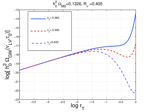
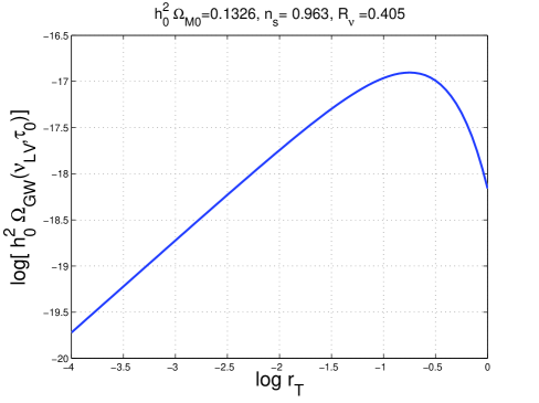
Figure 3: The spectral energy density of the relic gravitons in the context of the $\Lambda$CDM model evaluated at the Ligo/Virgo frequency as a function of the tensor-to-scalar ratio. To guide the intuition consider that (advanced) wide-band interferometers will achieve, optimistically, a sensitivity of $10^{-10}$ in $\Omega_{\mathrm{GW}}(\nu,\tau_{0})$. Taking into account the current bounds on $r_{\mathrm{T}}$ (see Tabs. 1 and 2) it is clear that the $\Lambda$CDM scenario is definitively too small to provide a serious target for wide-band detectors.

In Fig. 3, the common logarithm of the spectral energy density is illustrated as a function of the common logarithm of $r_{\mathrm{T}}$.

In Ref. [64] (see also [63, 65]) the current limits on the presence of an isotropic background of relic gravitons have been assessed. According to the Ligo collaboration (see Eq. (19) of Ref. [64]) the spectral energy density of a putative (isotropic) background of relic gravitons can be parametrized as:

$$\Omega_{\mathrm{GW}}(\nu,\tau_{0})=\Omega_{\mathrm{GW},\beta}\biggl{(}\frac{\nu}{100\,\mathrm{Hz}}\biggr{)}^{\beta+3}.$$ (1.12)

The parametrization of Eq. (1.12) fits very well with Fig. 3 where the pivot frequency $\nu_{\mathrm{LV}}=100\mathrm{Hz}$ coincides with the pivot frequency appearing in the parametrization (1.12). For the scale-invariant case (i.e. $\beta=-3$ in eq. (1.12)) the Ligo collaboration sets a $90\%$ upper limit of $1.20\times 10^{-4}$ on the amplitude appearing in Eq. (1.12), i.e. $\Omega_{\mathrm{GW},-3}$. Using different sets of data (see [63, 65]) the Ligo collaboration manages to improve the bound even by a factor $2$ getting down to $6.5\times 10^{-5}$. Thus Fig. 3 together with the upper limit of Eq. (1.12) shows that the current Ligo sensitivity is still too small to detect the relic graviton background arising within the $\Lambda$CDM paradigm.

1.5 Beyond the $\Lambda$CDM paradigm and high-frequency gravitons

In the case of an exactly scale invariant spectrum the correlation of the two (coaligned) LIGO detectors with central corner stations in Livingston (Lousiana) and in Hanford (Washington) might reach a sensitivity to a flat spectrum which is [68, 69, 70]

$$h_{0}^{2}\,\,\Omega_{\rm GW}(\nu_{\mathrm{LV}},\tau_{0})\simeq 6.5\times 10^{-11}\,\,\biggl{(}\frac{1\,\,\mathrm{yr}}{T}\biggr{)}^{1/2}\,\,\mathrm{SNR}^{2},\qquad\nu_{\mathrm{LV}}=0.1\,\,\mathrm{kHz}$$ (1.13)

where $T$ denotes the observation time and $\mathrm{SNR}$ is the signal to noise ratio. Equation (1.13) is in close agreement with the sensitivity of the advanced Ligo apparatus [55] to an exactly scale-invariant spectral energy density [71, 72, 73, 74]. Equation (1.13) together with the plots of Fig. 3 suggest that the relic graviton background predicted by the $\Lambda$CDM paradigm is not directly observable by wide-band interferometers in their advanced version.

CMB observations probe the aHz region of the spectral energy density of Fig. 2. Wide-band interferometers probe a frequency range between few Hz and $10$ kHz. In both ranges, the signal of the $\Lambda$CDM scenario might be too small to be directly detectable.

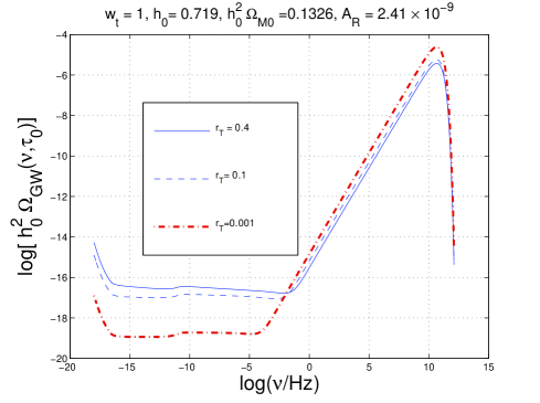
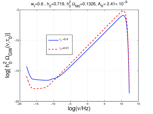
Figure 4: The spectral energy density of relic gravitons in the minimal T$\Lambda$CDM scenario where the post-inflationary thermal history contemplates a phase where the sound speed of the plasma $c_{\mathrm{st}}$ is close to the speed of light $c$. In the plot at the right $c_{\mathrm{st}}=c$ (corresponding to a constant barotropic index $w_{\mathrm{t}}=1$); in the plot at the left $c_{\mathrm{st}}=0.77\,c$ (corresponding to a constant barotropic index $w_{\mathrm{t}}=0.6$). In both plots the other cosmological parameters have been chosen to coincide with the best fit to the WMAP 5-yr data alone.

In Fig. 4 the spectral energy density is computed in an extension of the $\Lambda$CDM paradigm which has been dubbed tensor-$\Lambda$CDM (T$\Lambda$CDM for short) [40, 41]. In the T$\Lambda$CDM scenario the transition from the inflationary phase to the radiation-dominated epoch is mediated by a rather long stiff phase. By stiff phase we mean a phase where the total sound speed of the plasma is larger than the sound speed of a radiation-dominated plasma (i.e. $1/\sqrt{3}$ in natural units). In the simplest realization of the scenario the barotropic index $w_{\mathrm{t}}$ is constant during the stiff phase. For instance, in Fig. 4 the cases $w_{\mathrm{t}}=1$ and $w_{\mathrm{t}}=0.6$ have been illustrated. Since $w_{\mathrm{t}}$ denotes the ratio between the total pressure and the total energy density, it is rather plausible to demand that $w_{\mathrm{t}}\leq 1$. The latter requirement implies that the sound speed is always smaller than the speed of light. As suggested in [75] (see also [76, 77]) the presence of a stiff phase can have the effect of increasing the spectral energy density at high frequencies. The increase takes place for frequencies larger than the mHz and is typically maximal in the GHz region. The spectral energy densities illustrated in Fig. 4 suggest that it is not impossible to imagine situations where the spectral energy density of the relic gravitons satisfies all the constraints demanded by CMB physics but, at the same time, it is sufficiently large to be observed by wide-band interferometers. The results reported in Fig. 4 refer to the minimal T$\Lambda$CDM model where only one post-inflationary phase stiffer than radiation is contemplated. The barotropic index could have, however, a more complicated dependence. Already in the examples of Fig. 4 the numerical integration implies that the barotropic index does depend, effectively, upon the scale factor (see, e. g., discussions in section 6 on the transfer function for the spectral energy density).

The comparison of Fig. 2 and 4 suggests, in short, the following subjects of reflection:

• the theoretical error in the estimate of the spectral energy density increases with the frequency;

• departures from the standard post-inflationary thermal history can be directly imprinted in the primordial spectrum of the relic gravitons;

• in the incoming decade the observations of wide-band interferometers could be analyzed in conjunction with more standard data sets (i.e. CMB data supplemented by large-scale structure data and by the observations of type Ia supernovae) to constrain the spectral energy density of the relic gravitons both at small and at high frequencies.

The presence of post-inflationary phases stiffer than radiation is, after all, rather natural and this was the original spirit of [75]. We do not know which was the rate of the post-inflationary expansion and since guesses cannot substitute experiments it would be productive to use the T$\Lambda$CDM paradigm as reference model for a unified analysis of the low-frequency data stemming from CMB and of the high-frequency data provided by wide-band interferometers. Already in [75] (see also [76, 77]) a rather special candidate for a post-inflationary phase stiffer than radiation was the case when the sound speed equals the speed of light, i.e. the case when the energy density of the sources driving the geometry is dominated by the kinetic term of a (minimally coupled) scalar field. This particular case was also prompted by various classes of quintessence models. A specific example of this dynamics was provided in [78].

A more detailed account of the techniques leading to Fig. 4 will be swiftly presented in section 6 and can be found in [40, 41]. Without going through the details it is however important to stress that the calculations should be accurate enough not only in the high-frequency region but also in the low-frequency part of the spectrum. Indeed, as stressed above, one of the purposes of the T$\Lambda$CDM scenario is to convey the idea that low-frequency and high-frequency measurements of the relic graviton background can be analyzed in a single theoretical framework.

1.6 The millisecond pulsar bound and the nucleosynthesis constraint

The spectral energy density of the relic gravitons must be compatible not only with the CMB constraints (bounding, from above, the value of $r_{\mathrm{T}}$) but also with the pulsar timing bound[79, 80] and the big-bang nucleosynthesis constraints [81, 82, 83]. The pulsar timing bound demands

$$\Omega(\nu_{\mathrm{pulsar}},\tau_{0})<1.9\times 10^{-8},\qquad\nu_{\mathrm{pulsar}}\simeq\,10\,\mathrm{nHz},$$ (1.14)

where $\nu_{\mathrm{pulsar}}$ roughly corresponds to the inverse of the observation time during which the pulsars timing has been monitored. The spectral energy densities illustrated in Figs. 2 and 4 satisfy the pulsar timing bound.

The most constraining bound for the high-frequency branch of the relic graviton spectrum is represented by big-bang nucleosynthesis. Gravitons, being relativistic, can potentially increase the expansion rate at the BBN epoch. The increase in the expansion rate will affect, in particular, the synthesis of ${}^{4}\mathrm{He}$. To avoid the overproduction of ${}^{4}\mathrm{He}$ the expansion rate the number of relativistic species must be bounded from above.

The BBN bound is customarily expressed in terms of (equivalent) extra fermionic species. During the radiation-dominated era, the energy density of the plasma can be written as $\rho_{\mathrm{t}}=g_{\rho}(\pi^{2}/30)T^{4}$ where $T$ denotes here the common (thermodynamic) temperature of the various species. An (ultra)relativistic fermion species with two internal degrees of freedom and in thermal equilibrium contributes $2\cdot 7/8=7/4=1.75$ to $g_{\rho}$. Before neutrino decoupling the contributing relativistic particles are photons, electrons, positrons, and $N_{\nu}=3$ species of neutrinos, giving

$$g_{\rho}=\frac{11}{2}+\frac{7}{4}N_{\nu}=10.75.$$ (1.15)

The neutrinos have decoupled before electron-positron annihilation so that they do not contribute to the entropy released in the annihilation. While they are relativistic, the neutrinos still retain an equilibrium energy distribution, but after the annihilation their (kinetic) temperature is lower, $T_{\nu}=(4/11)^{1/3}T$. Thus

$$g_{\rho}=2+\frac{7}{4}N_{\nu}\left(\frac{T_{\nu}}{T}\right)^{4}=2+0.454N_{\nu}=3.36,$$ (1.16)

after electron-positron annihilation. By now assuming that there are some additional relativistic degrees of freedom, which also have decoupled by the time of electron-positron annihilation, or just some additional component $\rho_{X}$ to the energy density with a radiation-like equation of state (i.e. $p_{X}=\rho_{X}/3$), the effect on the expansion rate will be the same as that of having some (perhaps a fractional number of) additional neutrino species. Thus its contribution can be represented by replacing $N_{\nu}$ with $N_{\nu}+\Delta N_{\nu}$ in the above. Before electron-positron annihilation we have $\rho_{X}=(7/8)\Delta N_{\nu}\rho_{\gamma}$ and after electron-positron annihilation we have $\rho_{X}=(7/8)(4/11)^{4/3}\,\Delta N_{\nu}\,\rho_{\gamma}\simeq 0.227\,\Delta N_{\nu}\,\rho_{\gamma}$. The critical fraction of CMB photons can be directly computed from the value of the CMB temperature and it is notoriously given by $h_{0}^{2}\Omega_{\gamma}\equiv\rho_{\gamma}/\rho_{\mathrm{crit}}=2.47\times 10^{-5}$. If the extra energy density component has stayed radiation-like until today, its ratio to the critical density, $\Omega_{X}$, is given by

$$h_{0}^{2}\Omega_{X}\equiv h_{0}^{2}\frac{\rho_{X}}{\rho_{\mathrm{c}}}=5.61\times 10^{-6}\Delta N_{\nu}\biggl{(}\frac{h_{0}^{2}\Omega_{\gamma 0}}{2.47\times 10^{-5}}\biggr{)}.$$ (1.17)

If the additional species are relic gravitons, then [81, 82, 83]:

$$h_{0}^{2}\int_{\nu_{\mathrm{bbn}}}^{\nu_{\mathrm{max}}}\Omega_{{\rm GW}}(\nu,\tau_{0})d\ln{\nu}=5.61\times 10^{-6}\Delta N_{\nu}\biggl{(}\frac{h_{0}^{2}\Omega_{\gamma 0}}{2.47\times 10^{-5}}\biggr{)},$$ (1.18)

where $\nu_{\mathrm{bbn}}$ and $\nu_{\mathrm{max}}$ are given, respectively, by Eqs. (6.61) and (8.4). Thus the constraint of Eq. (1.18) arises from the simple consideration that new massless particles could eventually increase the expansion rate at the epoch of BBN. The extra-relativistic species do not have to be, however, fermionic [82] and therefore the bounds on $\Delta N_{\nu}$ can be translated into bounds on the energy density of the relic gravitons.

A review of the constraints on $\Delta N_{\nu}$ can be found in [82]. Depending on the combined data sets (i.e. various light elements abundances and different combinations of CMB observations), the standard BBN scenario implies that the bounds on $\Delta N_{\nu}$ range from $\Delta N_{\nu}\leq 0.2$ to $\Delta N_{\nu}\leq 1$. Similar figures, depending on the priors of the analysis, have been obtained in a more recent analysis [83]. All the relativistic species present inside the Hubble radius at the BBN contribute to the potential increase in the expansion rate and this explains why the integral in Eq. (1.18) must be performed from $\nu_{\mathrm{bbn}}$ to $\nu_{\mathrm{max}}$ (see also [76] where this point was stressed in the framework of a specific model). The existence of the exponential suppression for $\nu>\nu_{\mathrm{max}}$ (see Figs. 4) guarantees the convergence of the integral also in the case when the integration is performed up to $\nu\to\infty$. The constraint of Eq. (1.18) can be relaxed in some non-standard nucleosynthesis scenarios [82], but, in what follows, the validity of Eq. (1.18) will be enforced by adopting $\Delta N_{\nu}\simeq 1$ which implies, effectively

$$h_{0}^{2}\int_{\nu_{\mathrm{bbn}}}^{\nu_{\mathrm{max}}}\Omega_{{\rm GW}}(\nu,\tau_{0})d\ln{\nu}<5.61\times 10^{-6}\biggl{(}\frac{h_{0}^{2}\Omega_{\gamma 0}}{2.47\times 10^{-5}}\biggr{)}.$$ (1.19)

The spectral energy densities illustrated in Figs. 2 and 4 are both compatible with the big-bang nucleosynthesis bound. Thus the big-bang nucleosyntheis constraint does not forbid a potentially detectable signal in the high-frequency branch of the relic graviton spectrum. Potential deviations of the thermal history of the plasma must anyway occur before big-bang nucleosynthesis.

2 The polarization of relic gravitons and of relic photons

2.1 Basic notations

As discussed in the introduction, in the $\Lambda$CDM paradigm the background line element can be written

$$ds^{2}=\overline{g}_{\mu\nu}dx^{\mu}dx^{\nu}=a^{2}(\tau)[d\tau^{2}-\overline{\gamma}_{ij}(\vec{x})dx^{i}dx^{j}],$$ (2.1)

where, in the spatially flat case, $\overline{\gamma}_{ij}$ will coincide with $\delta_{ij}$ and the Friedmann-Lemaître equations can be written as

$$3{\mathcal{H}}^{2}=a^{2}\ell_{\mathrm{P}}^{2}\rho_{\mathrm{t}},$$ (2.2)

$$2({\mathcal{H}}^{2}-{\mathcal{H}}^{\prime})=a^{2}\ell_{\mathrm{P}}^{2}(\rho_{\mathrm{t}}+p_{\mathrm{t}}),$$ (2.3)

$$\rho_{\mathrm{t}}^{\prime}+3{\mathcal{H}}(\rho_{\mathrm{t}}+p_{\mathrm{t}})=0,$$ (2.4)

where ${\mathcal{H}}=a^{\prime}/a$; the prime denotes a derivation with respect to the conformal time coordinate $\tau$. The Hubble rate is customarily defined in the synchronous frame where the time coordinate (conventionally denoted by $t$) obeys $dt=a(\tau)d\tau$. Denoting with a dot a derivation with respect to the cosmic time $t$, $H=\dot{a}/a$, and, by definition, $H=a{\mathcal{H}}$. In Eqs. (2.2)–(2.4) $\rho_{\mathrm{t}}$ and $p_{\mathrm{t}}$ are, respectively, the total energy density and the total pressure of the plasma, i.e.

$$\rho_{\mathrm{t}}=\rho_{\mathrm{b}}+\rho_{\mathrm{c}}+\rho_{\gamma}+\rho_{\nu}+\rho_{\Lambda},\qquad\rho_{\mathrm{M}}=\rho_{\mathrm{b}}+\rho_{\mathrm{c}},$$ (2.5)

$$p_{\mathrm{t}}=\frac{\rho_{\gamma}}{3}+\frac{\rho_{\nu}}{3}-\rho_{\Lambda}.$$ (2.6)

The total matter fraction of the critical energy density, i.e. $\Omega_{\mathrm{M}0}=\rho_{\mathrm{M}0}/\rho_{\mathrm{crit}}$ consists of baryons and (i.e. $\rho_{\mathrm{b}}$) and cold dark matter particles (i.e. $\rho_{\mathrm{c}}$). In Tabs. 1 and 2 the values of $\Omega_{\mathrm{M}0}$ are given as they are inferred within the $\Lambda$CDM scenario. In similar terms $\Omega_{\Lambda}=\rho_{\Lambda}/\rho_{\mathrm{crit}}$ denotes the critical fraction of dark energy. In what follows, if not otherwise stated, the cosmological parameters will be fixed to the best fit of the WMAP-5yr data alone, i.e.

$$(\Omega_{\mathrm{b}0},\,\Omega_{\mathrm{c}0},\,\Omega_{\mathrm{\Lambda}},\,h_{0},\,n_{\mathrm{s}},\,\epsilon)=(0.0441,\,0.214,\,0.742,\,0.719,\,0.963,\,0.087).$$ (2.7)

where $\Omega_{\mathrm{b}0},\,\Omega_{\mathrm{c}0},\,\Omega_{\mathrm{\Lambda}}$ denote, respectively, the (present) critical fractions of baryons, CDM particles and dark energy; $h_{0}$ fixes the present value of the Hubble rate; $n_{\mathrm{s}}$, as already mentioned in section 1, is the spectral index of curvature perturbations and $\epsilon$ is the reionization optical depth.

At the beginning of the previous section we started by stressing analogies and differences between relic gravitons and relic photons. The most important one is that both gravitons and photons carry two polarizations. This observation is important for a quantitative understanding of the present endevours aimed at measuring the E-mode and the B-mode polarization of the CMB. In the present section the description of the polarization of the gravitons will be developed by stressing, when possible, the analogy with polarization observables of the electromagnetic field.

2.2 Linear and circular tensor polarizations

Recalling that $i,j,k,...$ are indices defined on the three-dimensional Euclidean sub-manifold, the tensor fluctuations of the geometry are parametrized in terms of the rank-two tensor $h_{ij}$

$$\delta_{\mathrm{t}}^{(1)}g_{ij}=-a^{2}\,\,h_{ij},\qquad h_{i}^{i}=\nabla_{i}h^{i}_{j}=0,$$ (2.8)

where $\nabla_{i}$ is the covariant derivative with respect to $\overline{\gamma}_{ij}$; if $\overline{\gamma}_{ij}=\delta_{ij}$, $\nabla_{i}=\partial_{i}$. In Eq. (2.8) the subscript refers to the tensor nature of the fluctuation while the superscript denotes the perturbative order. The tensor fluctuation $h_{ij}(\vec{x},\tau)$ can be decomposed in terms of the two linear polarizations, i.e.

$$h_{ij}(\vec{x},\tau)=\sum_{\lambda}h_{(\lambda)}(\vec{x},\tau)\epsilon_{ij}^{(\lambda)}(\hat{k}),\qquad\epsilon_{ij}^{(\lambda)}\epsilon_{ij}^{(\lambda^{\prime})}=2\delta^{\lambda\lambda^{\prime}},$$ (2.9)

where $\lambda=\oplus,\,\,\otimes$ denote the two polarizations and where

$$\epsilon_{ij}^{\oplus}(\hat{k})=(\hat{a}_{i}\hat{a}_{j}-\hat{b}_{i}\hat{b}_{j}),$$ (2.10)

$$\epsilon_{ij}^{\otimes}(\hat{k})=(\hat{a}_{i}\hat{b}_{j}+\hat{a}_{j}\hat{b}_{i}).$$ (2.11)

In Eqs. (2.10) and (2.11), $\hat{a}$, $\hat{b}$ and $\hat{k}=\vec{k}/|\vec{k}|$ represent a triplet of mutually orthogonal unit vectors, i.e.

$$\hat{a}\cdot\hat{b}=0,\qquad\hat{a}\cdot\hat{k}=0,\qquad\hat{b}\cdot\hat{k}=0.$$ (2.12)

If the direction of propagation coincides with the $\hat{z}$, the unit vectors $\hat{k}$, $\hat{a}$ and $\hat{b}$ can be chosen as:

$$\hat{k}=(0,\,0,\,1),\qquad\hat{a}=(1,\,0,\,0),\qquad\hat{b}=(0,\,1,\,0).$$ (2.13)

Using Eq. (2.13), Eqs. (2.10) and (2.11) become

$$\epsilon_{xx}^{\oplus}=1,\qquad\epsilon_{yy}^{\oplus}=-1,$$ (2.14)

$$\epsilon_{xy}^{\otimes}=1,\qquad\epsilon_{yx}^{\otimes}=1.$$ (2.15)

If $\hat{k}$ coincides with the radial direction, the unit vectors $\hat{k}$, $\hat{a}$ and $\hat{b}$ can be chosen, in spherical coordinates, as:

$$\hat{k}=(\sin{\vartheta}\cos{\varphi},\sin{\vartheta}\sin{\varphi},\cos{\vartheta}),$$ (2.16)

$$\hat{a}=(\cos{\vartheta}\cos{\varphi},\cos{\vartheta}\sin{\varphi},-\sin{\vartheta}),$$ (2.17)

$$\hat{b}=(\sin{\varphi},-\cos{\varphi},0).$$ (2.18)

Since $\epsilon_{ij}^{(\lambda)}(\hat{k})\epsilon_{ij}^{(\lambda^{\prime})}(\hat{k})=2\delta^{\lambda\lambda^{\prime}}$, it is straightforward to prove that

$$h_{ij}(\vec{x},\tau)h^{ij}(\vec{x},\tau)=2[h_{\otimes}(\vec{x},\tau)^{2}+h_{\oplus}(\vec{x},\tau)^{2}].$$ (2.19)

As in the case of electromagnetic waves, it is often desirable to pass from the linear to the circular polarizations:

$$\epsilon_{ij}^{(\mathrm{L})}(\hat{k})=\frac{1}{\sqrt{2}}[\epsilon_{ij}^{\oplus}(\hat{k})+i\epsilon_{ij}^{\otimes}(\hat{k})],$$ (2.20)

$$\epsilon_{ij}^{(\mathrm{R})}(\hat{k})=\frac{1}{\sqrt{2}}[\epsilon_{ij}^{\oplus}(\hat{k})-i\epsilon_{ij}^{\otimes}(\hat{k})].$$ (2.21)

Equations (2.20) and (2.21) also imply that $\epsilon_{ij}^{(\mathrm{L})*}=\epsilon_{ij}^{(\mathrm{R})}$ and $\epsilon_{ij}^{(\mathrm{R})*}=\epsilon_{ij}^{(\mathrm{L})}$. A rotation of $\hat{a}$ and $\hat{b}$ in the plane orthogonal to $\hat{k}=\vec{k}/|\vec{k}|$

$$\hat{a}^{\prime}=\cos{\alpha}\,\hat{a}+\sin{\alpha}\,\hat{b},$$ (2.22)

$$\hat{b}^{\prime}=-\sin{\alpha}\,\hat{a}+\cos{\alpha}\,\hat{b},$$ (2.23)

implies, using Eqs. (2.10) and (2.11),

$$\tilde{\epsilon}_{ij}^{\oplus}=\epsilon_{ij}^{\oplus}\cos{2\alpha}+\epsilon_{ij}^{\otimes}\sin{2\alpha},$$ (2.24)

$$\tilde{\epsilon}_{ij}^{\otimes}=-\epsilon_{ij}^{\oplus}\sin{2\alpha}+\epsilon_{ij}^{\otimes}\cos{2\alpha},$$ (2.25)

where the tilde denotes the two transformed (linear) polarizations. Under the transformation given in Eqs. (2.22) and (2.23) the two circular polarizations defined in Eqs. (2.20) and (2.21) transform as

$$\tilde{\epsilon}_{ij}^{(\mathrm{L})}(\hat{k})=e^{-2i\alpha}\epsilon_{ij}^{(\mathrm{L})}(\hat{k}),\qquad\tilde{\epsilon}_{ij}^{(\mathrm{R})}(\hat{k})=e^{2i\alpha}\epsilon_{ij}^{(\mathrm{R})}(\hat{k}).$$ (2.26)

The transformation properties of the circular polarization under a rotation in the plane orthogonal to the direction of propagation are closely analog to the transformation properties, under the same rotation, of the polarization of the electromagnetic field. This analogy will now be exploited to introduce the E-mode and B-mode polarization.

Before proceeding with the discussion it is appropriate to recall a very basic aspect of rotations which can have, however, some confusing impact of the polarization analysis especially in the case of the tensor modes. Consider, for simplicity, a coordinate system characterized by two basis vectors, i.e. $\hat{e}_{x}=\hat{r}\cos{\vartheta}$ and $\hat{e}_{y}=\hat{r}\sin{\vartheta}$. If we now perform a clockwise (i.e. right-handed) rotation of the axes $\hat{e}_{x}$ and $\hat{e}_{y}$, the rotated basis $(\hat{e}^{\prime}_{x},\,\hat{e}^{\prime}_{y})$ will be given as in Eqs. (2.22) and (2.23) by replacing $(\hat{a}^{\prime},\,\hat{b}^{\prime})\to(\hat{e}^{\prime}_{x},\,\hat{e}^{\prime}_{y})$ and $(\hat{a},\,\hat{b})\to(\hat{e}_{x},\,\hat{e}_{y})$. Some authors, for different reasons, instead of rotating the coordinate system prefer to rotate the polarization vector. If angles are in the right-handed sense for the rotation of the axes, they are in the left-handed sense for the rotation of the vectors.

2.3 Polarization of the CMB radiation field

The radiation field can be described by the polarization tensor, i.e.

$$\rho_{ij}=E_{i}E_{j}^{*},$$ (2.27)

where $E_{i}$ and $E_{j}$ are the electric components of the radiation field. Assuming, for sake of simplicity, that the radiation field propagate along the $\hat{z}$ axis, then the various entries of $\rho_{ij}$ can be written in a matrix form

$$\rho_{ij}=\left(\matrix{|E_{x}|^{2}&E_{x}\,E_{y}^{*}&\cr E_{y}\,E_{x}^{*}&|E_{y}|^{2}&\cr}\right),$$ (2.28)

where $x$ and $y$ denote the components of the electric field orthogonal to the direction of propagation coinciding, in this set-up, with the third Cartesian axis. A full description of the radiation field can be achieved by studying the four Stokes parameters [84] conventionally named $I$, $Q$, $U$ and $V$:

$$I=|E_{x}|^{2}+|E_{y}|^{2},\qquad V=2\,\mathrm{Im}[E_{x}^{*}\,E_{y}],$$ (2.29)

$$U=2\,\mathrm{Re}[E_{x}^{*}\,E_{y}],\qquad Q=|E_{x}|^{2}-|E_{y}|^{2}.$$ (2.30)

It is immediate, from the definitions (2.29) and (2.30), to write the intensities of the radiation field along the different Cartesian axis as a function of the Stokes parameters, i.e.

$$|E_{x}|^{2}=\frac{I+Q}{2},\qquad|E_{x}|^{2}=\frac{I-Q}{2},$$ (2.31)

$$E_{x}\,E_{y}^{*}=\frac{U+iV}{2},\qquad E_{x}^{*}\,E_{y}=\frac{U-iV}{2}.$$ (2.32)

Equations (2.31) and (2.32) can be inserted back into Eq. (2.28) with the result that

$$\rho_{ij}=\frac{1}{2}\left(\matrix{I+Q&U-iV\cr U+iV&I-Q\cr}\right)=\overline{P}_{ij}+P_{ij},$$ (2.33)

where

$$\overline{P}_{ij}=\frac{1}{2}\left(\matrix{I&-iV\cr iV&I\cr}\right),\qquad P_{ij}=\frac{1}{2}\left(\matrix{Q&U\cr U&-Q\cr}\right).$$ (2.34)

From Eq. (2.33) it also follows that

$$\rho_{ij}=\frac{1}{2}\left(I\,{\bf 1}+U\,\sigma_{1}+V\,\sigma_{2}+Q\,\sigma_{3}\right)$$ (2.35)

where ${\bf 1}$ is the $2\times 2$ unit matrix and

$$\sigma_{1}=\left(\matrix{0&1\cr 1&0\cr}\right),\qquad\sigma_{2}=\left(\matrix{0&-i\cr i&0\cr}\right),\qquad\sigma_{3}=\left(\matrix{1&0\cr 0&-1\cr}\right),$$ (2.36)

are the Pauli matrices. Consider now a rotation of an angle $\alpha$ on the plane orthogonal to the direction of propagation of the monochromatic wave. It is easy to show that $I$ and $V$ are left invariant while $Q$ and $U$ do transform by a rotation of $2\alpha$. By indicating with a tilde the transformed Stokes parameters the result can be expressed as

$$\tilde{Q}=\cos{2\alpha}\,Q+\sin{2\alpha}\,U,\qquad\tilde{U}=-\sin{2\alpha}\,Q+\cos{2\alpha}\,U.$$ (2.37)

Equations (2.24)–(2.25) and (2.37) express the fact that the polarization of the graviton and of the radiation field do change for a rotation on the plane orthogonal to the direction of propagation of the radiation (either gravitational or electromagnetic). It is possible to construct polarization observables which are invariant for rotations on the plane orthogonal to the direction of propagation of the radiation: because of their properties under parity transformations they are called E-and B-modes.

2.4 E- and B-modes

The fluctuations of the geometry induce fluctuations of the Stokes parameters whose spectral properties are, ultimately, the aim of CMB polarization experiments. In general terms the fluctuation of each Stokes parameter can be written as

$$\Delta_{\mathrm{I}}(\hat{n},\tau) = \Delta^{(\mathrm{T})}_{\mathrm{I}}(\hat{n},\tau)+\Delta^{(\mathrm{S})}_{\mathrm{I}}(\hat{n},\tau)+\Delta^{(\mathrm{V})}_{\mathrm{I}}(\hat{n},\tau),$$ (2.38)

$$\Delta_{\mathrm{Q}}(\hat{n},\tau) = \Delta^{(\mathrm{T})}_{\mathrm{Q}}(\hat{n},\tau)+\Delta^{(\mathrm{S})}_{\mathrm{Q}}(\hat{n},\tau)+\Delta^{(\mathrm{V})}_{\mathrm{Q}}(\hat{n},\tau),$$ (2.39)

$$\Delta_{\mathrm{U}}(\hat{n},\tau) = \Delta^{(\mathrm{T})}_{\mathrm{U}}(\hat{n},\tau)+\Delta^{(\mathrm{S})}_{\mathrm{U}}(\hat{n},\tau)+\Delta^{(\mathrm{V})}_{\mathrm{U}}(\hat{n},\tau).$$ (2.40)

In Eqs. (2.38)–(2.40) the superscript reminds that the various fluctuations of the Stokes parameters are induced, respectively, by the tensor, scalar and vector modes of the geometry. While some of the results of the present section will be generally valid, the focus, in what follows, will be on the tensor contribution. Defining the two linear combinations

$$\Delta_{\pm}(\hat{n},\tau)=\Delta_{\mathrm{Q}}(\hat{n},\tau)\pm i\Delta_{\mathrm{U}}(\hat{n},\tau),$$ (2.41)

and denoting with a tilde the transformed quantities, Eq. (2.37) implies that $\Delta_{\pm}(\hat{n},\tau)$ transform as

$$\tilde{\Delta}_{\pm}(\hat{n},\tau)=e^{\mp 2i\alpha}\,\Delta_{\pm}(\hat{n},\tau).$$ (2.42)

In more general terms, consider a generic function of $\hat{n}$ (be it $f(\hat{n})$). Under a rotation of an angle $\alpha$ on the plane orthogonal to $\hat{n}$, $f(\hat{n})$ is said to transform as a function of (integral) spin-weight $\pm s$ provided

$$\tilde{f}(\hat{n})=e^{\mp is\alpha}f(\hat{n}).$$ (2.43)

In other words $\Delta_{+}(\hat{n})$ and $\Delta_{-}(\hat{n})$ transform, respectively, as functions of spin weight $+2$ and $-2$. The circular polarizations of the gravitons introduced in Eqs. (2.24)–(2.25) transform, respectively, as functions of spin weight $+2$ and $-2$. The brightness perturbations for the intensity of the radiation field (i.e. $\Delta_{\mathrm{I}}(\hat{n})$) transform, on the contrary, as quantities of spin weight $0$. The fluctuations in the intensity of the radiation field, being a spin-0 quantity, can be expanded in ordinary spherical harmonics as

$$\Delta_{\mathrm{I}}(\hat{n},\tau) = \sum_{\ell\,m}a^{(\mathrm{T})}_{\ell\,m}Y_{\ell\,m}(\hat{n}),$$

$$a^{(\mathrm{T})}_{\ell\,m} = \int d\hat{n}Y_{\ell\,m}^{*}(\hat{n})\Delta_{\mathrm{I}}(\hat{n},\tau)$$ (2.44)

The spin-s quantity will naturally be expanded in terms of a generalization of the ordinary spherical harmonics which are called spin-s spherical harmonics or also spin-weighted spherical harmonics. Owing to this observation, $\Delta_{\pm}(\hat{n},\tau)$ can be expanded in terms of spin-$\pm 2$ spherical harmonics ${}_{\pm 2}Y_{\ell\,m}(\hat{n})$, i.e.

$$\Delta_{\pm}(\hat{n},\tau)=\sum_{\ell\,m}a_{\pm 2,\,\ell\,m}\,{}_{\pm 2}Y_{\ell\,m}(\hat{n}).$$ (2.45)

Given a quantity of spin-weight $s$ it is possible to construct quantities of spin-weight $0$ by the repeated use of appropriate differential operators which can either raise or lower the spin-weight of a given function (see subsection 2.5 for a specific discussion). Consequently, from $\Delta_{+}(\hat{n},\tau)$ and $\Delta_{-}(\hat{n},\tau)$ it is possible to construct two fluctuations of spin $0$ which can be eventually expanded in ordinary spherical harmonics. By demanding that the two fluctuations of spin-weight $0$ are eigenstates of parity the E- and B-modes are defined as

$$\Delta_{\mathrm{E}}(\hat{n},\tau) = \sum_{\ell\,m}\overline{N}_{\ell}^{-1}\,a^{(\mathrm{E})}_{\ell\,m}\,Y_{\ell\,m}(\hat{n}),\qquad\overline{N}_{\ell}=\sqrt{\frac{(\ell-2)!}{(\ell+2)!}},$$

$$\Delta_{\mathrm{B}}(\hat{n},\tau) = \sum_{\ell\,m}\overline{N}_{\ell}^{-1}\,a^{(\mathrm{B})}_{\ell\,m}\,Y_{\ell\,m}(\hat{n}),$$ (2.46)

where

$$a^{(\mathrm{E})}_{\ell\,m}=-\frac{1}{2}(a_{2,\,\ell m}+a_{-2,\,\ell m}),\qquad a^{(\mathrm{B})}_{\ell\,m}=\frac{i}{2}(a_{2,\,\ell m}-a_{-2,\,\ell m}).$$ (2.47)

From $a^{(\mathrm{T})}_{\ell\,m}$, $a^{(\mathrm{E})}_{\ell\,m}$ and $a^{(\mathrm{B})}_{\ell\,m}$ the angular power spectra can be defined. In particular the EE, BB, TT and TE angular power spectra are given by:

$$C_{\ell}^{(\mathrm{EE})} = \frac{1}{2\ell+1}\sum_{m=-\ell}^{\ell}\langle a^{(\mathrm{E})*}_{\ell m}\,a^{(\mathrm{E})}_{\ell m}\rangle,\qquad C_{\ell}^{(\mathrm{BB})}=\frac{1}{2\ell+1}\sum_{m=-\ell}^{\ell}\langle a^{(\mathrm{B})*}_{\ell m}\,a^{(\mathrm{B})}_{\ell m}\rangle,$$ (2.48)

$$C_{\ell}^{(\mathrm{TT})} = \frac{1}{2\ell+1}\sum_{m=-\ell}^{\ell}\langle a^{(\mathrm{T})*}_{\ell m}\,a^{(\mathrm{T})}_{\ell m}\rangle,\qquad C_{\ell}^{(\mathrm{TE})}=\frac{1}{2\ell+1}\sum_{m=-\ell}^{\ell}\langle a^{(\mathrm{T})*}_{\ell m}\,a^{(\mathrm{E})}_{\ell m}\rangle,$$ (2.49)

where $\langle...\rangle$ denotes the ensemble average. Two further power spectra can be defined and they are:

$$C_{\ell}^{(\mathrm{EB})}=\frac{1}{2\ell+1}\sum_{m=-\ell}^{\ell}\langle a^{(\mathrm{E})*}_{\ell m}\,a^{(\mathrm{B})}_{\ell m}\rangle,\qquad C_{\ell}^{(\mathrm{TB})}=\frac{1}{2\ell+1}\sum_{m=-\ell}^{\ell}\langle a^{(\mathrm{T})*}_{\ell m}\,a^{(\mathrm{B})}_{\ell m}\rangle.$$ (2.50)

Overall, the existence of linear polarization allows for 6 different power spectra.

In the minimal version of the $\Lambda$CDM paradigm the adiabatic fluctuations of the scalar curvature lead to a polarization which is characterized exactly by the condition $a_{2,\,\ell m}=a_{-2,\,\ell m}$, i.e. $a_{\ell m}^{(\mathrm{B})}=0$. This observation implies that, in the $\Lambda$CDM scenario, the non-vanishing angular power spectra are given by the TT, EE and TE correlations. In the T$\Lambda$CDM scenario the TT, EE and TE angular power spectra are supplemented by a specific prediction for the B-mode autocorrelation (see section 7).

2.5 Spin-2 spherical harmonics

Spherical harmonics of higher spin appear in matrix elements calculations in nuclear physics (see e.g. the classic treatise of Blatt and Weisskopf [85], and, in a similar perspective the book of Edmonds [86]). The comprehensive treatments of Biedenharn and Louk [87] and of Varshalovich et al. [88] can also be usefully consulted.

The spin-s harmonics have been introduced, in their present form, by Newman and Penrose [89] and their group theoretical interpretation has been discussed in [90]. The spin-s spherical harmonics have been applied to the discussion of CMB polarization induced by relic gravitons in a number of papers [91, 92, 93]. They are rather crucial in the formulation of the so-called total angular momentum approach. Discussions of the spin-weighted spherical harmonics in a cosmological context can also be found in [94, 95]. The spin weighted spherical harmonics will now be introduced by following the spirit of Ref. [90] which has been also used, with different conventions, in [91]. In subsection 2.6 the (equivalent) approach of [92, 93] will be more specifically outlined.

Th functions ${}_{\pm 2}Y_{\ell\,m}(\hat{n})$ appearing in Eq. (2.45) are the spin-2 spherical harmonics [90]. Consider the representations of the operator specifying three-dimensional rotations, i.e. $\hat{R}$; this problem is usually approached within the matrix element, i.e. ${\cal D}_{m\,m^{\prime}}^{(j)}(R)=\langle j,\,m^{\prime}|\hat{R}|j,\,m\rangle$ where $j$ denotes the eigenvalue of $J^{2}$ and $m$ denotes the eigenvalue of $J_{z}$. Now, if we replace $m^{\prime}\to-{\rm s}$, $j\to\ell$, we have the definition of spin-s spherical harmonics in terms of the ${\cal D}_{-{\rm s},\,m}^{(\ell)}(\alpha,\beta,0)$, i.e.

$${}_{\rm s}Y_{\ell\,m}(\alpha,\beta)=\sqrt{\frac{2\ell+1}{4\pi}}{\cal D}_{-{\rm s},\,m}^{(\ell)}(\alpha,\beta,0),$$ (2.51)

where $\alpha$, $\beta$ and $\gamma$ (set to zero in the above definition) are the Euler angles defined as in [96]. If $s=0$, ${\cal D}_{0,\,m}^{(\ell)}(\alpha,\beta,0)=\sqrt{(2\ell+1)/4\pi}Y_{\ell\,m}(\alpha,\beta)$ where $Y_{\ell\,m}(\alpha,\beta)$ are the ordinary spherical harmonics. The spin-s spherical harmonics can be obtained from the spin-0 spherical harmonics by using repeatedly the differential operators:

$$K_{+}^{(\mathrm{s})}(\hat{n})=-(\sin\vartheta)^{s}\,\left[\partial_{\vartheta}+{i\over\sin\theta}\partial_{\varphi}\right]\frac{1}{(\sin\vartheta)^{s}},$$ (2.52)

$$K_{-}^{(\mathrm{s})}(\hat{n})=-\frac{1}{(\sin{\vartheta})^{s}}\,\left[\partial_{\vartheta}-{i\over\sin\vartheta}\partial_{\varphi}\right](\sin\vartheta)^{s}.$$ (2.53)

The notation spelled out in Eqs. (2.52) and (2.53) (which is not usual) will be employed to emphasize the interpretation of $K_{\pm}^{(\mathrm{s})}$ as ladder operators (see [90]). The operator $K_{+}^{(\mathrm{s})}$ raises the spin weight of a function by one unit. Consider, therefore, the ordinary spherical harmonics $Y_{\ell\,m}(\hat{n})$ defined as

$$Y_{\ell\,m}(\hat{n}) = N_{\ell}^{m}P_{\ell}^{m}(\mu)e^{im\varphi},\qquad N_{\ell}^{m}=\sqrt{\frac{2\ell+1}{4\pi}}\sqrt{\frac{(\ell-m)!}{(\ell+m)!}},\qquad\mu=\cos{\vartheta}$$ (2.54)

$$P_{\ell}^{m}(\mu) = (-1)^{m}(1-\mu^{2})^{m/2}\frac{d^{m}}{d\mu^{m}}P_{\ell}(\mu),\qquad P_{\ell}^{-m}(\mu)=(-1)^{m}\frac{(\ell-m)!}{(\ell+m)!}P_{\ell}^{m}(\mu),$$ (2.55)

where $P_{\ell}(\mu)$ are the Legendre polynomials and $P_{\ell}^{m}(\mu)$ the associated Legendre functions. It is appropriate to mention here that the factor $(-1)^{m}$ (i.e. Condon-Shortley phase) can either be included in the normalization factor $N_{\ell}^{m}$ or (as it has been done) in the definition of the associated Legendre functions appearing in Eq. (2.55). When using the recurrence relations of the associated Legendre functions the Condon-Shortley phase introduces a sign difference every time $m$ is odd. The conventions expressed by Eqs. (2.54) and (2.55) will be followed throughout the present discussion and, in particular, in section 7 where the correlation functions of the E-modes and of the B-modes will be specifically computed with different techniques.

According to Eq. (2.43), $Y_{\ell\,m}$ transform with $s=0$, i.e. they have spin weight $0$. By applying once $K_{+}^{(0)}(\hat{n})$ to $Y_{\ell\,m}(\hat{n})$ we do get a function of spin weight $1$, i.e.

$$K_{+}^{(0)}(\hat{n})Y_{\ell\,m}(\hat{n})=-\biggl{[}\partial_{\vartheta}+\frac{i}{\sin{\vartheta}}\partial_{\varphi}\biggr{]}Y_{\ell\,m}(\hat{n}).$$ (2.56)

We can then apply once more $K_{+}^{(1)}(\hat{n})$ to $K_{+}^{(0)}(\hat{n})Y_{\ell\,m}(\hat{n})$. The result of this simple manipulation will be

$$K_{+}^{(1)}(\hat{n})\,[K_{+}^{(0)}(\hat{n})Y_{\ell\,m}(\hat{n})]=\biggl{[}\partial_{\vartheta}^{2}-\cot{\vartheta}\partial_{\vartheta}-\frac{\partial_{\varphi}^{2}}{\sin^{2}{\vartheta}}+\frac{2i}{\sin{\vartheta}}(\partial_{\vartheta}\partial_{\varphi}-\cot{\vartheta}\partial_{\varphi})\biggr{]}Y_{\ell\,m}(\hat{n}).$$ (2.57)

The right hand side of Eq. (2.57) is ${}_{+2}Y_{\ell\,m}(\vartheta,\varphi)$ (up to an overall normalization). Including the appropriate normalization factor, ${}_{\pm 2}Y_{\ell\,m}(\vartheta,\varphi)$, i.e. the spherical harmonics of spin weight $s=\pm 2$ are given by:

$${}_{\pm 2}Y_{\ell\,m}(\vartheta,\varphi)=\sqrt{\frac{(\ell-2)!}{(\ell+2)!}}\biggl{[}\partial_{\vartheta}^{2}-\cot{\vartheta}\partial_{\vartheta}-\frac{\partial_{\varphi}^{2}}{\sin^{2}{\vartheta}}\pm\frac{2i}{\sin{\vartheta}}(\partial_{\vartheta}\partial_{\varphi}-\cot{\vartheta}\partial_{\varphi})\biggr{]}Y_{\ell\,m}(\hat{n}).$$ (2.58)

The spin weights $s=\pm 2$ are both needed since the transformation of the polarization involve both spin weights (see Eq. (2.45)). In fact, since ${}_{\pm 2}Y_{\ell\,m}(\vartheta,\varphi)$ form a complete and orthogonal basis on the sphere, i.e.

$$\int d\hat{n}\,_{s}Y^{*}_{\ell^{\prime}\,m^{\prime}}(\vartheta,\varphi)_{s}Y_{\ell\,m}(\vartheta,\varphi)=\delta_{\ell^{\prime}\,\ell}\,\delta_{m^{\prime}m},$$ (2.59)

$$\sum_{\ell,m}\,{}_{s}Y_{\ell\,m}^{*}(\vartheta,\varphi)_{s}Y_{\ell\,m}(\vartheta^{\prime},\varphi^{\prime})=\delta(\varphi-\varphi^{\prime})\,\delta(\cos\vartheta-\cos\vartheta^{\prime}),$$ (2.60)

$\Delta_{\pm}(\hat{n},\tau)$ can be expanded in terms of ${}_{\pm 2}Y_{\ell\,m}(\vartheta,\varphi)$ as in Eq. (2.45). The coefficients off the expansion will be given by

$$a_{2,\,\ell\,m} = \int d\hat{n}\,\,_{2}Y_{\ell\,m}^{*}(\hat{n})\Delta_{+}(\hat{n},\tau),$$ (2.61)

$$a_{-2,\,\ell\,m} = \int d\hat{n}\,\,_{-2}Y_{\ell\,m}^{*}(\hat{n})\Delta_{-}(\hat{n},\tau).$$ (2.62)

Integrating by parts in Eqs. (2.61) and (2.62) allows for a different form of the expansion coefficients $a_{\pm 2,\,\ell\,m}$:

$$a_{2,\,\ell\,m} = \overline{N}_{\ell}\int d\hat{n}Y_{\ell\,m}^{*}K^{(1)}_{-}(\hat{n})[K^{(2)}_{-}(\hat{n})\Delta_{+}(\hat{n},\tau)],$$ (2.63)

$$a_{-2,\,\ell\,m} = \overline{N}_{\ell}\int d\hat{n}Y_{\ell\,m}^{*}K^{(-1)}_{-}(\hat{n})[K^{(-2)}_{+}(\hat{n})\Delta_{-}(\hat{n},\tau)],$$ (2.64)

where, as already mentioned, $\overline{N}_{\ell}=\sqrt{(\ell-2)!/(\ell+2)!}$. In Eqs. (2.63) and (2.64) there appear only ordinary (i.e. spin-weight $0$) spherical harmonics. This occurrence suggests a complementary approach to the problem: instead of expanding $\Delta_{\pm}(\hat{n},\tau)$ in terms of spin-2 spherical harmonics, fluctuations of spin-weight $0$ can be directly constructed (in real space) from $\Delta_{\pm}(\hat{n},\tau)$ by repeated application of the ladder operators defined in Eqs. (2.52) and (2.53).

The E-mode and B-mode polarization in real space are then, in explicit terms:

$$\Delta_{\mathrm{E}}(\hat{n},\tau)=-\frac{1}{2}\{K^{(1)}_{-}(\hat{n})[K^{(2)}_{-}(\hat{n})\Delta_{+}(\hat{n},\tau)]+K^{(-1)}_{-}(\hat{n})[K^{(-2)}_{+}(\hat{n})\Delta_{-}(\hat{n},\tau)]\},$$ (2.65)

$$\Delta_{\mathrm{B}}(\hat{n},\tau)=\frac{i}{2}\{K^{(1)}_{-}(\hat{n})[K^{(2)}_{-}(\hat{n})\Delta_{+}(\hat{n},\tau)]-K^{(-1)}_{-}(\hat{n})[K^{(-2)}_{+}(\hat{n})\Delta_{-}(\hat{n},\tau)]\}.$$ (2.66)

The quantities $\Delta_{\mathrm{E}}(\hat{n},\tau)$ and $\Delta_{\mathrm{B}}(\hat{n},\tau)$ can be expanded in terms of ordinary spherical harmonics, as already suggested in Eq. (2.46):

$$\Delta_{\mathrm{E}}(\hat{n},\tau)=\sum_{\ell\,m}\overline{N}_{\ell}^{-1}\,a^{(\mathrm{E})}_{\ell\,m}\,Y_{\ell\,m}(\hat{n}),\qquad\Delta_{\mathrm{B}}(\hat{n},\tau)=\sum_{\ell\,m}\overline{N}_{\ell}^{-1}\,a^{(\mathrm{B})}_{\ell\,m}\,Y_{\ell\,m}(\hat{n}),$$ (2.67)

The “electric” and “magnetic” components of polarization are eigenstates of parity and may be defined, from $a_{\pm,\,\,\ell\,m}$ as already mentioned in Eq. (2.47):

$$a_{\ell m}^{(\rm E)}=-\frac{1}{2}(a_{2,\ell m}+a_{-2,\ell m}),\qquad a_{\ell m}^{(\rm B)}=\frac{i}{2}(a_{2,\ell m}-a_{-2,\ell m}).$$ (2.68)

Under parity the components appearing in Eqs. (2.68) transform

$$a_{\ell m}^{(\rm E)}\to(-1)^{\ell}\,\,a_{\ell m}^{\rm E},\qquad a_{\ell m}^{(\rm B)}\to(-1)^{\ell+1}\,\,a_{\ell m}^{\rm B}.$$ (2.69)

Therefore, the E-modes have the same parity of the temperature correlations which have, in turn, the same parity of conventional spherical harmonics, i.e. $(-1)^{\ell}$. On the contrary, the B-modes have $(-1)^{\ell+1}$ parity. The same analysis can be directly performed in real space, i.e. using Eqs. (2.65) and (2.66). Denoting the radial direction with $\hat{n}$ and the tangential directions with $\hat{e}_{1}$ and $\hat{e}_{2}$, the ladder operators defined in Eqs. (2.52) and (2.53) are consistent with the following choice of $\hat{e}_{1}$ and $\hat{e}_{2}$:

$$\hat{e}_{1}=(\cos{\vartheta}\cos{\varphi},-\cos{\vartheta}\sin{\varphi},-\sin{\vartheta}),\qquad\hat{e}_{2}=(-\sin{\varphi},-\cos{\varphi},0).$$ (2.70)

A parity transformation (i.e. a space inversion) implies, in spherical coordinates, that

$$r\to r,\qquad\vartheta\to\pi-\vartheta,\qquad\varphi\to\pi+\varphi.$$ (2.71)

The transformation (2.71) implies that the two basis vectors defined in Eq. (2.70) transform as $\hat{e}_{1}\to\hat{e}_{1}$ and $\hat{e}_{2}\to-\hat{e}_{2}$, i.e. while $\hat{e}_{1}$ does not change $\hat{e}_{2}$ flips its sign under space inversion. It follows that space-inversion does not flip the sign of $\Delta_{\mathrm{E}}(\hat{n})$ but it does flip the sign of $\Delta_{\mathrm{B}}(\hat{n})$, i.e. under the transformation (2.71), $\Delta_{\mathrm{E}}(\hat{n})\to\Delta_{\mathrm{E}}(\hat{n})$ while $\Delta_{\mathrm{B}}(\hat{n})\to-\Delta_{\mathrm{B}}(\hat{n})$.

Using Eqs. (2.63) and (2.64) inside Eq. (2.68) a more explicit expression for $a_{\ell m}^{(\rm E)}$ and $a_{\ell m}^{(\rm B)}$ can be obtained and it is:

$$a_{\ell m}^{(\rm B)}=\frac{i\,\overline{N}_{\ell}}{2}\int d\hat{n}Y_{\ell\,m}(\hat{n})^{*}\{K^{(1)}_{-}(\hat{n})[K^{(2)}_{-}(\hat{n})\Delta_{+}(\hat{n},\tau)]-K^{(-1)}_{-}(\hat{n})[K^{(-2)}_{+}(\hat{n})\Delta_{-}(\hat{n},\tau)]\},$$ (2.72)

$$a_{\ell m}^{(\rm E)}=-\frac{\overline{N}_{\ell}}{2}\int d\hat{n}Y_{\ell\,m}(\hat{n})^{*}\{K^{(1)}_{-}(\hat{n})[K^{(2)}_{-}(\hat{n})\Delta_{+}(\hat{n},\tau)]+K^{(-1)}_{-}(\hat{n})[K^{(-2)}_{+}(\hat{n})\Delta_{-}(\hat{n})]\}.$$ (2.73)

The contribution of long wavelength gravitons to Eqs. (2.72) and (2.73) will be discussed in section 7. It is often useful to observe that the differential operators appearing in the definition of the spin-weighted spherical harmonics (see, e.g. Eq. (2.58)) can be expressed in terms of the usual differential operators arising in the theory of the orbital angular momentum in non-relativistic quantum mechanics (see, e. g. [96]). Indeed, recalling that

$$L_{\pm}=e^{\pm i\varphi}[\pm\partial_{\vartheta}+i\cot{\vartheta}\,\partial_{\varphi}],\qquad L_{z}=-i\partial_{\varphi},$$ (2.74)

$$L^{2}=\frac{1}{2}(L_{+}\,L_{-}+L_{-}\,L_{+})+L_{z}^{2},$$ (2.75)

it can be easily deduced that

$$\cot{\vartheta}\partial_{\varphi}=-\frac{i}{2}[e^{-i\varphi}\,L_{+}+e^{i\varphi}\,L_{-}],$$ (2.76)

$$\partial_{\vartheta}\partial_{\varphi}=\frac{i}{2}[e^{-i\varphi}\,L_{+}\,L_{z}-e^{i\varphi}\,L_{-}\,L_{z}]$$ (2.77)

$$-\cot{\vartheta}\partial_{\vartheta}-\frac{\partial_{\varphi}^{2}}{\sin^{2}{\vartheta}}=L^{2}+\partial_{\vartheta}^{2}.$$ (2.78)

Equations (2.76)–(2.78) allow often to express combinations of spin-$2$ spherical harmonics in terms of ordinary (i.e. spin-weight $0$) spherical harmonics using the properties of the ladder operators associated to the (orbital) angular momentum, i.e. $L_{\pm}$:

$$L_{\pm}Y_{\ell\,m}=\sqrt{\ell(\ell+1)-m(m\pm 1)}Y_{\ell,m\pm 1},\qquad L_{z}Y_{\ell\,m}=mY_{\ell\,m},\qquad L^{2}Y_{\ell\,m}=\ell(\ell+1)Y_{\ell\,m},$$ (2.79)

where $L_{\pm}$ and $L_{z}$ obey the well known commutation relations $[L_{\pm},L_{z}]=\mp L_{\pm}$ and $[L_{+},L_{-}]=2L_{z}$.

Looking at Eq. (2.79) it is tempting draw a parallel between the (orbital) ladder operators and the ladder operators raising (or lowering) the spin weight of a given function (see Eqs. (2.52) and (2.53). This problem has been discussed and solved in [90]. It is possible to formulate the parallel in terms of a putative $O(4)$ group. Half of the generators will be connected with the orbital angular momentum operators, while the other half will allow to increase (or decrease) the spin weight of a given function. The two sets of generators commute. The operators $K_{\pm}^{(\mathrm{s})}$ are not directly, though, the ladder operators stemming from the second set of generators. This has to do with the fact that in Eq. (2.51) the third Euler angle (i.e. $\gamma$) has been fixed to zero. The $K_{\pm}^{(\mathrm{s})}$ are ladder operators defined within a putative $O(4)$ group in the case $\gamma\neq 0$. When $\gamma\to 0$ the dependence upon $\gamma$ drops and we are left with Eqs. (2.52) and (2.53).

2.6 Polarization on the 2-sphere

In a more geometric perspective, the spin-2 harmonics are introduced by describing the polarization tensor on the 2-sphere which represents the microwave sky. In Eq. (2.34) the tensor $P_{ij}$ describes the properties of the radiation field and it is symmetric and trace-free (i.e. $P_{ij}=P_{ji}$ and $P_{i}^{i}=0$). Equation (2.34) holds in flat space-time. On the 2-sphere the line element can be written as

$$ds^{2}=d\vartheta^{2}+\sin^{2}{\vartheta}\varphi^{2},\qquad g_{\vartheta\vartheta}=1,\qquad g_{\varphi\varphi}=\sin^{2}{\vartheta}.$$ (2.80)

The polarization matrix $P_{ij}$ will now be generalized as

$$P_{ab}(\hat{n})=\frac{1}{2}\left(\begin{array}[]{cc}Q(\hat{n})&-U(\hat{n})\sin\vartheta\\ -U(\hat{n})\sin\vartheta&-Q(\hat{n})\sin^{2}\vartheta\\ \end{array}\right),$$ (2.81)

satisfying $P_{ab}=P_{ba}$, and $g^{ab}P_{ab}=0$, where $\hat{n}$ is a unit vector in the direction $(\vartheta,\varphi)$. The sign of the off-diagonal entries in Eq. (2.81) is opposite with respect to the one obtained in Eq. (2.34). This is just because we want to match with the conventions adopted, for instance, in [93, 94, 95]. To avoid possible confusions, furthermore, the Latin indices $a,\,b,\,c,\,d,....$ run over the two-dimensional space.

As already mentioned, for scalar functions defined on the 2-sphere, such as the temperature anisotropies, the spherical harmonic functions $Y_{\ell m}(\hat{n})$ are the complete orthonormal basis. For the $2\times 2$ tensors defined on the 2-sphere, such as $P_{ab}$ in Eq.(2.81), the complete orthonormal set of tensor spherical harmonics can be written as [93, 94, 95]:

$$Y_{(\ell m)ab}^{\rm G}=N_{\ell}\left(\nabla_{a}\nabla_{b}Y_{(\ell m)}-{1\over 2}g_{ab}\nabla_{c}\nabla^{c}Y_{(\ell m)}\right),$$ (2.82)

$$Y_{(\ell m)ab}^{\rm C}={N_{\ell}\over 2}\left(\vphantom{1\over 2}\nabla_{a}\nabla_{c}Y_{(\ell m)}\epsilon^{c}{}_{b}+\nabla_{b}\nabla_{c}Y_{(\ell m)}\epsilon^{c}{}_{a}\right),$$ (2.83)

where $\nabla$, in this subsection, denotes a covariant derivation on the 2-sphere, e.g.

$$\nabla_{a}\nabla_{b}Y_{(\ell m)}=\partial_{a}\partial_{b}Y_{(\ell m)}-\Gamma_{ab}^{c}\partial_{c}Y_{(\ell m)},\qquad\nabla_{c}\nabla^{c}Y_{(\ell m)}=\partial_{c}\partial^{c}Y_{(\ell m)}+\Gamma_{ca}^{c}\partial^{a}Y_{(\ell m)}.$$ (2.84)

$$\Gamma_{ac}^{c}=\frac{1}{2}\,g^{cd}(-\partial_{d}g_{ab}+\partial_{b}g_{dc}+\partial_{c}g_{bd}).$$ (2.85)

Using Eq. (2.80) into Eq. (2.85), the Christoffel connections $\Gamma_{ab}^{c}$ on the 2-sphere are

$$\Gamma_{\varphi\vartheta}^{\varphi}=\frac{1}{\tan{\vartheta}},\qquad\Gamma_{\varphi\varphi}^{\vartheta}=-\sin{\vartheta}\cos{\vartheta}.$$ (2.86)

In Eq. (2.83) the normalization factor is given by $N_{\ell}\equiv\sqrt{{2(\ell-2)!/(\ell+2)!}}$, while

$$\epsilon^{a}\,_{b}=\left(\begin{array}[]{cc}0&\sin\theta\\ -1/\sin\theta&0\\ \end{array}\right),$$ (2.87)

is the Levi-Civita symbol on the 2-sphere. The differential operators acting in Eqs. (2.82) and (2.83) are interpreted as a generalized gradient and curl operators, i.e.

$$\nabla_{ab}^{(\mathrm{G})}=\nabla_{a}\nabla_{b}-{1\over 2}g_{ab}\nabla_{c}\nabla^{c},\qquad\nabla_{ab}^{(\mathrm{C})}=\epsilon^{c}{}_{b}\nabla_{a}\nabla_{c}+\epsilon^{c}{}_{a}\nabla_{b}\nabla_{c}$$ (2.88)

The explicit form of the various components of $Y^{\mathrm{G}}_{(\ell m)ab}$ and $Y^{\mathrm{C}}_{ab}$ can be computed. For instance using Eqs. (2.82), (2.84) and (2.86), the explicit components of $Y^{\mathrm{G}}_{(\ell m)ab}$:

$$Y_{(\ell m)\vartheta\vartheta}^{(\mathrm{G})}(\vartheta,\varphi)=\frac{N_{\ell}}{2}\biggl{[}\partial_{\vartheta}^{2}Y_{(\ell m)}-\frac{\partial_{\varphi}^{2}Y_{(\ell m)}}{\sin^{2}{\vartheta}}-\frac{\partial_{\vartheta}Y_{(\ell m)}}{\tan{\vartheta}}\biggr{]},$$ (2.89)

$$Y_{(\ell m)\varphi\varphi}^{(\mathrm{G})}(\vartheta,\varphi)=\frac{N_{\ell}}{2}[\partial_{\varphi}^{2}Y_{(\ell m)}-\sin^{2}{\vartheta}\partial_{\vartheta}^{2}\,\,Y_{(\ell m)}+\sin{\vartheta}\cos{\vartheta}\partial_{\vartheta}Y_{(\ell m)}]$$ (2.90)

$$Y_{(\ell m)\vartheta\varphi}^{(\mathrm{G})}(\vartheta,\varphi)=N_{\ell}\biggl{[}\partial_{\vartheta}\partial_{\varphi}Y_{(\ell m)}-\frac{\partial_{\varphi}Y_{(\ell m)}}{\tan{\vartheta}}\biggr{]}.$$ (2.91)

The expressions obtained in Eqs. (2.89), (2.90) and (2.91) can be simplified by recalling Eqs. (2.74), (2.75) and (2.79). Equations (2.89), (2.90) and (2.91) can be simply rewritten as

$$Y_{(\ell m)\vartheta\vartheta}^{(\mathrm{G})}(\vartheta,\varphi)=\frac{N_{\ell}}{2}[2\,\partial_{\vartheta}^{2}\,Y_{(\ell m)}+\ell(\ell+1)Y_{(\ell m)}],$$ (2.92)

$$Y_{(\ell m)\varphi\varphi}^{(\mathrm{G})}(\vartheta,\varphi)=-\frac{N_{\ell}}{2}[2\partial_{\vartheta}^{2}Y_{(\ell m)}+\ell(\ell+1)Y_{(\ell m)}],$$ (2.93)

$$Y_{(\ell m)\vartheta\varphi}^{(\mathrm{G})}(\vartheta,\varphi)=miN_{\ell}\biggl{[}\partial_{\vartheta}\partial_{\varphi}Y_{(\ell m)}-\frac{Y_{(\ell m)}}{\tan{\vartheta}}\biggr{]}.$$ (2.94)

The same exercise can be conducted for the various components of $Y_{(\ell m)ab}^{(\mathrm{C})}(\vartheta,\varphi)$. The $Y_{(\ell m)ab}^{(\mathrm{G})}$ and $Y_{(\ell m)ab}^{(\mathrm{C})}$ can be written in the form of $2\times 2$ matrices:

$$Y_{(\ell m)ab}^{\mathrm{G}}(\hat{n})={N_{\ell}\over 2}\left(\begin{array}[]{cc}W_{(\ell m)}(\hat{n})&X_{(\ell m)}(\hat{n})\sin\vartheta\\ \vskip 6.0pt\cr X_{(\ell m)}(\hat{n})\sin\vartheta&-W_{(\ell m)}(\hat{n})\sin^{2}\vartheta\\ \end{array}\right),$$ (2.95)

and as

$$Y_{(\ell m)ab}^{(\mathrm{C})}(\hat{n})={N_{\ell}\over 2}\left(\begin{array}[]{cc}-X_{(\ell m)}(\hat{n})&W_{(\ell m)}(\hat{n})\sin\vartheta\\ \vskip 6.0pt\cr W_{(\ell m)}(\hat{n})\sin\theta&X_{(\ell m)}(\hat{n})\sin^{2}\vartheta\\ \end{array}\right),$$ (2.96)

where

$$W_{(\ell m)}(\hat{n})=[2\partial^{2}_{\vartheta}+\ell(\ell+1)]Y_{(\ell m)}(\hat{n}),\qquad X_{(\ell m)}(\hat{n})={2im\over\sin\vartheta}(\partial_{\vartheta}-\cot\vartheta)Y_{(\ell m)}(\hat{n}).$$ (2.97)

In terms of the spin-2 harmonics ${}_{\pm 2}Y_{(lm)}(\hat{n})$

$$W_{(\ell m)}(\hat{n})\pm iX_{(\ell m)}(\hat{n})=\sqrt{{(\ell+2)!\over(\ell-2)!}}\,_{\pm 2}Y_{(\ell m)}(\hat{n}),$$ (2.98)

which is Eq. (2.58). Using the orthonormality of the spherical harmonics $Y_{\ell m}(\hat{n})$ it is easy to prove the orthonormality conditions, i.e.

$$\int d\hat{n}\,Y_{(\ell m)ab}^{(\mathrm{G})\,*}(\hat{n})\,Y_{(\ell^{\prime}m^{\prime})}^{(\mathrm{G})\,\,ab}(\hat{n})=\int d\hat{n}\,Y_{(\ell m)ab}^{(\mathrm{C})\,*}(\hat{n})\,Y_{(\ell^{\prime}m^{\prime})}^{(\mathrm{C})\,\,ab}(\hat{n})=\delta_{\ell^{\prime}\ell}\delta_{mm^{\prime}},$$

$$\int d\hat{n}\,Y_{(\ell m)ab}^{(\mathrm{G})\,*}(\hat{n})\,Y_{(\ell^{\prime}m^{\prime})}^{(\mathrm{C})\,\,ab}(\hat{n})=0,$$ (2.99)

where $d\hat{n}=\sin{\vartheta}d\vartheta d\varphi$ denotes, as usual, the integration over the solid angle. Since $Y_{(\ell m)ab}^{\mathrm{G}}$ and $Y_{(\ell m)ab}^{\mathrm{C}}$ form an appropriate orthonormal basis, the polarization can be expanded as

$$P_{ab}(\hat{n})=\sum_{\ell=2}^{\infty}\sum_{m=-\ell}^{\ell}\left[a_{\ell m}^{(\mathrm{G})}Y_{(\ell m)ab}^{(\mathrm{G})}(\hat{n})+a_{\ell m}^{(\mathrm{C})}Y_{(\ell m)ab}^{(\mathrm{C})}(\hat{n})\right],$$ (2.100)

where expansion coefficients $a_{\ell m}^{(\mathrm{G})}$ and $a_{\ell m}^{(\mathrm{C})}$ represent the electric and magnetic type components of the polarization, respectively. Note that the sum starts from $\ell=2$, since relic gravitons generate only perturbations of multipoles from the quadrupoles up. The expansion coefficients are obviously

$$a_{\ell m}^{(\mathrm{G})}=\int\,d\hat{n}\,{P}_{ab}(\hat{n})Y_{(\ell m)}^{(\mathrm{G})\,ab\,*}(\hat{n}),\quad a_{\ell m}^{(\mathrm{C})}=\int d\hat{n}\,{P}_{ab}(\hat{n})Y_{(\ell m)}^{{(\mathrm{C})}\,ab\,*}(\hat{n}).$$ (2.101)

In the notations of [91] the $a_{\ell m}^{(\mathrm{G})}$ and $a_{\ell m}^{(\mathrm{C})}$ can be related to the $a_{\ell m}^{(\mathrm{E})}$ and $a_{\ell m}^{(\mathrm{B})}$ already introduced in Eq. (2.68). The relation between the two sets of expansion coefficients is simply:

$$a_{\ell m}^{(\mathrm{G})}=\frac{\overline{N}_{\ell}}{N_{\ell}}a_{\ell m}^{(\mathrm{E})}=\frac{a_{\ell m}^{(\mathrm{E})}}{\sqrt{2}},\qquad a_{\ell m}^{(\mathrm{C})}=\frac{\overline{N}_{\ell}}{N_{\ell}}a_{\ell m}^{(\mathrm{B})}=\frac{a_{\ell m}^{(\mathrm{B})}}{\sqrt{2}},$$ (2.102)

The two approaches to the spin weighted spherical harmonics described in the present section are equivalent and can be used interchangeably depending upon the specific problem.

3 The action of the relic gravitons

3.1 Second-order fluctuations of the Einstein-Hilbert action

By perturbing the Einstein-Hilbert action, to second-order in the amplitude of the tensor fluctuations we have, formally, that:

$$\delta_{\mathrm{t}}^{(2)}S=-\frac{1}{16\pi G}\int d^{4}x[\delta_{\mathrm{t}}^{(2)}(\sqrt{-g})\,\overline{R}+\sqrt{-\overline{g}}\,\delta_{\mathrm{t}}^{(2)}R+\delta_{\mathrm{t}}^{(1)}(\sqrt{-g})\,\,\delta_{\mathrm{t}}^{(1)}R],$$ (3.1)

where $\overline{R}$ denotes the background Ricci scalar; $\delta^{(1)}R$ and $\delta^{(2)}R$ denote respectively, the first and second-order fluctuations of $R=g^{\mu\nu}R_{\mu\nu}$. In Eq. (3.1) the possible coupling to the anisotropic stress has been neglected. This is customary during the early evolution of the geometry since, in the context of the $\Lambda$CDM paradigm, during the early inflationary phase the sources of anisotropic stress can be safely ignored unless the number of effective e-folds is close to minimal. Later on the anisotropic stress of the fluid plays a role and cannot be neglected at least if we aim at a reasonable quantitative discussion of the relic graviton spectrum (see also section 1 and Fig. 3). By introducing the first-order fluctuations of the background geometry $\overline{g}_{\mu\nu}$ we have that

$$g_{\mu\nu}=\overline{g}_{\mu\nu}+H_{\mu\nu},$$ (3.2)

$$g^{\mu\nu}=\overline{g}^{\mu\nu}-H^{\mu\nu}+H^{\mu\alpha}H_{\alpha}^{\nu}$$ (3.3)

$$\sqrt{-g}=\sqrt{-\overline{g}}\biggl{[}1+\frac{1}{2}\overline{g}^{\rho\alpha}H_{\rho\alpha}-\frac{1}{4}\overline{g}^{\rho\alpha}\overline{g}^{\nu\sigma}H_{\alpha\nu}H_{\sigma\rho}+\frac{1}{8}\overline{g}^{\rho\alpha}\overline{g}^{\nu\sigma}H_{\rho\alpha}H_{\nu\sigma}\biggr{]}.$$ (3.4)

Recalling now Eqs. (2.1) and (2.8), Eqs. (3.2)–(3.4) become

$$\delta_{\mathrm{t}}^{(1)}g^{ij}=\frac{h^{ij}}{a^{2}},\qquad\delta_{\mathrm{t}}^{(2)}g^{ij}=-\frac{h^{i}_{k}h^{kj}}{a^{2}}.$$ (3.5)

The first- and second-order fluctuations of the Christoffel connections are:

$$\delta_{\rm t}^{(1)}\Gamma_{ij}^{0}=\frac{1}{2}(h_{ij}^{\prime}+2{\cal H}h_{ij}),\qquad\delta_{\rm t}^{(1)}\Gamma_{i0}^{j}=\frac{1}{2}{h_{i}^{j}}^{\prime},\qquad\delta_{\rm t}^{(1)}\Gamma_{ij}^{k}=\frac{1}{2}(\partial_{i}h^{k}_{j}+\partial_{j}h_{i}^{k}-\partial^{k}h_{ij}),$$

$$\delta_{\rm t}^{(2)}\Gamma_{i0}^{j}=-\frac{1}{2}h^{ik}h_{kj}^{\prime},\qquad\delta_{\rm t}^{(2)}\Gamma_{ij}^{k}=\frac{1}{2}h^{i\ell}[\partial_{\ell}h_{jk}-\partial_{k}h_{j\ell}-\partial_{j}h_{k\ell}],$$ (3.6)

where the prime denotes a derivation with respect to the conformal time coordinate. Using the result of Eq. (3.6) the first- and second- order fluctuations of the Ricci tensor can be written in explicit terms:

$$\delta_{\rm t}^{(1)}R_{ij} = \frac{1}{2}[h_{ij}^{\prime\prime}+2{\cal H}h_{ij}^{\prime}-\nabla^{2}h_{ij}]+({\cal H}^{\prime}+2{\cal H}^{2})h_{ij},$$ (3.7)

$$\delta_{\rm t}^{(2)}R_{00} = \frac{1}{4}h_{ij}^{\prime}{h^{ij}}^{\prime}-\frac{{\cal H}}{2}h_{ij}{h^{ij}}^{\prime}+\frac{1}{2}h^{ij}\nabla^{2}h_{ij},$$ (3.8)

$$\delta_{\rm t}^{(2)}R_{ij} = \frac{1}{2}h^{k\ell}[\partial_{k}\partial_{\ell}h_{ij}-\partial_{k}\partial_{j}h_{\ell i}-\partial_{k}\partial_{i}h_{j\ell}]$$ (3.9)

$$- \frac{1}{2}\partial_{j}[h^{k\ell}(\partial_{\ell}h_{ik}-\partial_{k}h_{\ell i}-\partial_{i}h_{k\ell})]-\frac{{\cal H}}{2}h^{k\ell}h_{k\ell}^{\prime}\delta_{ij}$$

$$+ \frac{{\cal H}}{2}h^{\ell}_{j}h_{\ell i}^{\prime}+\frac{{\cal H}}{2}h^{\ell}_{i}h_{\ell j}^{\prime}-\frac{1}{4}{h^{k}_{j}}^{\prime}h_{ik}^{\prime}-\frac{{\cal H}}{2}{h^{k}_{j}}^{\prime}h_{ik}-\frac{1}{4}{h^{k}_{i}}^{\prime}h_{kj}^{\prime}-\frac{{\cal H}}{2}{h^{k}_{i}}^{\prime}h_{kj}$$

$$- \frac{1}{4}[\partial_{i}h_{k}^{\ell}+\partial_{k}h^{\ell}_{i}-\partial^{\ell}h_{ik}][\partial_{\ell}h^{k}_{j}+\partial_{j}h^{k}_{\ell}-\partial^{k}h_{j\ell}].$$

The Ricci scalar is zero to first order in the tensor fluctuations, i.e. $\delta_{\rm t}^{(1)}R=0$. This is due to the traceless nature of these fluctuations. To second-order, however, $\delta_{\rm t}^{(2)}R\neq 0$ and its form is:

$$\delta_{\rm t}^{(2)}R = \frac{1}{a^{2}}\biggl{\{}\frac{3}{4}h_{k\ell}^{\prime}{h^{k\ell}}^{\prime}+{\cal H}h_{k\ell}^{\prime}h^{k\ell}+\frac{1}{2}h^{k\ell}\nabla^{2}h_{k\ell}-\frac{1}{4}\partial_{i}h^{k\ell}\partial^{i}h_{k\ell}\biggr{\}}$$ (3.10)

$$+ \frac{1}{a^{2}}\biggl{\{}-\frac{1}{2}\partial_{i}[h^{k\ell}(\partial_{\ell}h^{i}_{k}-\partial_{k}h_{\ell}^{i}-\partial^{i}h_{k\ell})]$$

$$- \frac{1}{4}[\partial_{i}h^{\ell}_{k}\partial_{\ell}h^{k}_{i}-\partial_{i}h^{\ell}_{k}\partial^{k}h_{i\ell}+\partial_{k}h^{\ell i}\partial_{\ell}h^{k}_{i}-\partial^{\ell}h_{ik}\partial^{i}h^{k}_{\ell}+\partial^{\ell}h_{ik}\partial^{k}h_{i\ell}]\biggr{\}}.$$

Using the results of Eqs. (3.7)–(3.10) into Eq. (3.1) the second-order action for the tensor modes reads, up total derivatives,

$$S_{\mathrm{gw}}=\delta_{\mathrm{t}}^{(2)}S=\frac{1}{8\ell_{\mathrm{P}}^{2}}\int d^{4}x\sqrt{-\overline{g}}\,\,\overline{g}^{\mu\nu}\,\,\partial_{\mu}h_{ij}\partial_{\nu}h^{ij},$$ (3.11)

where, as already mentioned in section 1,

$$\ell_{\mathrm{P}}^{2}=8\pi G=\frac{1}{\overline{M}_{\mathrm{P}}^{2}}=\frac{8\pi}{M_{\mathrm{P}}^{2}},\qquad M_{\mathrm{P}}=1.221\times 10^{19}\,\mathrm{GeV}.$$ (3.12)

3.2 Lagrangian densities

The action (3.11) can be written in various ways which differ by the addition (or subtraction) of a total conformal time derivative. Recalling the standard notations

$$S_{\mathrm{gw}}=\int d\tau L_{\mathrm{gw}}(\tau),\qquad L_{\mathrm{gw}}(\tau)=\int d^{3}x{\mathcal{L}}_{\mathrm{gw}}(\vec{x},\tau),$$ (3.13)

the Langrangian density ${\mathcal{L}}^{(1)}(\vec{x},\tau)$ can be recast in the form

$${\mathcal{L}}_{\mathrm{gw}}^{(1)}(\vec{x},\tau)=\frac{a^{2}(\tau)}{2}[(\partial_{\tau}h)^{2}-\overline{\gamma}^{ij}\nabla_{i}h\nabla_{j}h],$$ (3.14)

where the canonical amplitude $h$ has been introduced

$$h=\frac{h_{\otimes}}{\sqrt{2}\ell_{\mathrm{P}}}=\frac{h_{\oplus}}{\sqrt{2}\ell_{\mathrm{P}}}.$$ (3.15)

By now introducing the canonical amplitude as $ah=\mu$, Eq. (3.13) can be transformed as

$${\mathcal{L}}^{(2)}_{\mathrm{gw}}(\vec{x},\tau)=\frac{1}{2}[(\partial_{\tau}\mu)^{2}+{\mathcal{H}}^{2}\mu^{2}-2{\mathcal{H}}\mu\mu^{\prime}-\overline{\gamma}^{ij}\nabla_{i}\mu\nabla_{j}\mu].$$ (3.16)

If a total $\tau$ derivative is dropped, an equivalent form of the Lagrangian density can be obtained

$${\mathcal{L}}_{\mathrm{gw}}^{(3)}(\vec{x},\tau)=\frac{1}{2}[(\partial_{\tau}\mu)^{2}+({\mathcal{H}}^{2}+{\mathcal{H}}^{\prime})\mu^{2}-\overline{\gamma}^{ij}\nabla_{i}\mu\nabla_{j}\mu].$$ (3.17)

All the three Lagrangian densities of Eqs. (3.14), (3.16) and (3.17) lead to the same Euler-Lagrange equations.

3.3 Hamiltonian densities

In Eq. (3.14) the canonical field is $h$ and the canonical momentum is $\Pi=ah^{\prime}$. Conversely, in Eq. (3.16) the canonical field is $\mu$ and the associated canonical momentum is $\tilde{\pi}=\mu^{\prime}-{\mathcal{H}}\mu$. Finally, according to Eq. (3.17) the canonical momentum is $\pi=\mu^{\prime}$ while the canonical field is always $\mu$. The three Lagrangian densities of Eqs. (3.14), (3.16) and (3.17) will then lead to three corresponding Hamiltonians, i.e.

$$H_{\mathrm{gw}}^{(1)}(\tau)=\frac{1}{2}\int d^{3}x\biggl{[}\frac{\Pi^{2}}{a^{2}}+a^{2}\overline{\gamma}^{ij}\nabla_{i}h\nabla_{j}h\biggr{]},$$ (3.18)

$$H_{\mathrm{gw}}^{(2)}(\tau)=\frac{1}{2}\int d^{3}x[\tilde{\pi}^{2}+2{\mathcal{H}}\mu\tilde{\pi}+\overline{\gamma}^{ij}\nabla_{i}\mu\nabla_{j}\mu],$$ (3.19)

$$H_{\mathrm{gw}}^{(3)}(\tau)=\frac{1}{2}\int d^{3}x\biggl{[}\pi^{2}-\frac{a^{\prime\prime}}{a}\mu^{2}+\overline{\gamma}^{ij}\nabla_{i}\mu\nabla_{j}\mu\biggr{]},$$ (3.20)

The Hamiltonians of Eqs. (3.18), (3.19) and (3.20) are related by successive canonical transformations. To prove this statement it is enough to show that Eq. (3.19) can be obtained from Eq. (3.18) by means of an appropriate canonical tansformation and that, in turn, Eq. (3.20) can be obtained from Eq. (3.19) through another canonical transformation. To pass from the Hamiltonian of Eq. (3.18) to Eq. (3.19) it is practical to consider a generating functional depending upon the new canonical fields (i.e. $\mu$) and upon the old canonical momenta (i.e. $\Pi$):

$${\mathcal{G}}_{(1)\to(2)}[\mu,\Pi]=-\int\frac{\mu\,\Pi}{a}d^{3}x.$$ (3.21)

By taking the functional derivative of ${\mathcal{G}}_{(1)\to(2)}[\mu,\Pi]$ with respect to $\Pi$ and with respect to $\mu$ we get, up to a sign, the connection between the new and old pivot variables, namely:

$$h=-\frac{\delta{\mathcal{G}}_{(1)\to(2)}}{\delta\Pi}=\frac{\mu}{a},\qquad\tilde{\pi}=-\frac{\delta{\mathcal{G}}_{(1)\to(2)}}{\delta\mu}=\frac{\Pi}{a}.$$ (3.22)

Since the generating functional depends explicitly upon time, the new Hamiltonian will be related to the old one through a partial time derivative of the generating functional, i.e.

$$H_{\mathrm{gw}}^{(2)}(\tau)=H_{\mathrm{gw}}^{(1)}(\tau)+\frac{\partial{\mathcal{G}}_{(1)\to(2)}}{\partial\tau},$$ (3.23)

as it can be explicitly verified by using Eqs. (3.18), (3.19) and (3.21) into Eq. (3.23). A further canonical transformation allows to go from Eq. (3.19) to (3.20); the relevant generating functional is

$${\mathcal{G}}_{(2)\to(3)}[\mu,\pi]=-\int d^{3}x\biggl{(}\mu\pi-\frac{{\mathcal{H}}\mu^{2}}{2}\biggr{)},$$ (3.24)

depending upon the old coordinates (i.e. $\mu$) and upon the new momenta (i.e. $\pi$). The relations between the new and old variables are given by

$$\tilde{\pi}=\frac{\delta{\mathcal{G}}_{(2)\to(3)}}{\delta\mu}=\pi-{\mathcal{H}}\mu,\qquad\mu=\frac{\delta{\mathcal{G}}_{(2)\to(3)}}{\delta\pi}=\mu,$$ (3.25)

stipulating that, in this case, the canonical momentum gets shifted by ${\mathcal{H}}\mu$ while the canonical field is left invariant. Since the generating functional depends explicitly upon the conformal time coordinate, we will simply have that

$$H_{\mathrm{gw}}^{(3)}(\tau)=H_{\mathrm{gw}}^{(2)}(\tau)+\frac{\partial{\mathcal{G}}_{(2)\to(3)}}{\partial\tau}$$ (3.26)

as it can be explicitly verified by using Eqs. (3.19), (3.20) and (3.25) into Eq. (3.26).

3.4 Evolution equations in different regimes

From Eq. (3.11) the evolution equations of $h_{i}^{j}$ will be given by

$${h_{i}^{j}}^{\prime\prime}+2{\mathcal{H}}{h_{i}^{j}}^{\prime}-\nabla^{2}h_{i}^{j}=0.$$ (3.27)

The canonical field $h$ (see Eq. (3.15)) will also obey Eq. (3.27). The Hamilton equations derived from Eq. (3.18) read:

$$h^{\prime}=\frac{\Pi}{a^{2}},\qquad\Pi^{\prime}=a^{2}\nabla^{2}h,$$ (3.28)

which has exactly the same content as Eq. (3.27). In similar terms the Hamilton’s equations can be derived from Eq. (3.19) and the result is

$$\mu^{\prime}=\tilde{\pi}+{\mathcal{H}}\mu,\qquad\tilde{\pi}^{\prime}=-{\mathcal{H}}\tilde{\pi}+\nabla^{2}\mu.$$ (3.29)

Bearing in mind that $ah=\mu$, Eqs. (3.28) and (3.29) all reduce to Eq. (3.27) since the different Hamiltonians are related by canonical transformations. The same conclusion follows by deriving the Hamilton’s equations using Eq. (3.20). It is practical, for some applications, to change the time parametrization. For instance, in terms of the rescaled time coordinate $\sigma$ we will have that the evolution for the canonical amplitude $h$ obeys the simple equation

$$\frac{\partial^{2}h}{\partial\sigma^{2}}-a^{4}\nabla^{2}h=0,\qquad a^{2}(\tau)d\tau=d\sigma.$$ (3.30)

Before concluding this section it should be pointed out that Eq. (3.27) is accurate as long as the sources of anisotropic stress are totally absent. This approximation is, strictly speaking, unrealistic. Indeed we do know that there are sources of anisotropic stress. Typically, after neutrino decoupling, the neutrinos free stream and the effective energy-momentum tensor acquires, to first-order in the amplitude of the plasma fluctuations, an anisotropic stress, i.e.

$$\delta T_{i}^{j}=-\delta p\delta_{i}^{j}+\Pi_{i}^{j}$$ (3.31)

where $\Pi_{i}^{j}$ is the contribution of the anisotropic stress, satisfying $\nabla_{i}\Pi_{j}^{i}=0$ and $\Pi_{i}^{i}=0$. The presence of the anisotropic stress clearly affects the evolution of the tensor modes. To obtain the wanted equation we perturb the Einstein equations to first-order and we get:

$${h_{i}^{j}}^{\prime\prime}+2{\mathcal{H}}{h_{i}^{j}}^{\prime}-\nabla^{2}h_{i}^{j}=-16\pi Ga^{2}\Pi_{i}^{j}.$$ (3.32)

This form of the evolution equation for the tensor modes is the one required to compute the effects related to the finite value of the anisotropic stress.

4 Quantization of the tensor modes

There are analogies between the quantum state of relic gravitons and the quantum treatment of visible light. Quantum effects are not crucial to treat first-order interference of the radiation field (i.e. Young interferometry) [97]. First-order interference in quantum optics correspond to the calculation of the two-point function of the relic gravitons. Quantum effects arise, in optics, from second-order interference, i.e. when computing (and measuring) the interference between the intensities of the radiation field. Second-order interference effects are associated with the possibilities of counting photons and have been pioneered by Hanbury-Brown and Twiss in the early fifties [97, 98]. Hanbury-Brown-Twiss interferometry is based on photon counting statistics.

Having said that we are not even close (experimentally) to study graviton counting statistics (as we do it with the photons), second order interference effects would allow, in principle, to assess the coherence properties of relic graviton backgrounds. The quantum state of the relic gravitons can be described in terms of a generalized coherent state usually called squeezed state. Squeezed states can be described in terms of quadrature operators where one of the modes of the radiation field is always broadened by the time evolution, while the other one is squeezed.

4.1 Heisenberg description

The quantization of the canonical Hamiltonian of Eq. (3.20) is performed by promoting the normal modes of the action to field operators in the Heisenberg description and by imposing (canonical) equal-time commutation relations:

$$[\hat{\mu}(\vec{x},\tau),\hat{\pi}(\vec{y},\tau)]=i\delta^{(3)}(\vec{x}-\vec{y}).$$ (4.1)

The operator corresponding to the Hamiltonian (3.20) becomes:

$$\hat{H}(\tau)=\frac{1}{2}\int d^{3}x\biggl{[}\hat{\pi}^{2}-\frac{a^{\prime\prime}}{a}\hat{\mu}^{2}+(\partial_{i}\hat{\mu})^{2}\biggr{]}.$$ (4.2)

In Fourier space the quantum fields $\hat{\mu}$ and $\hat{\pi}$ can be expanded as

$$\hat{\mu}(\vec{x},\tau)=\frac{1}{2(2\pi)^{3/2}}\int d^{3}k\biggl{[}\hat{\mu}_{\vec{k}}e^{-i\vec{k}\cdot\vec{x}}+\hat{\mu}_{\vec{k}}^{\dagger}\,e^{i\vec{k}\cdot\vec{x}}\biggr{]},\qquad\hat{\pi}(\vec{y},\tau)=\frac{1}{2(2\pi)^{3/2}}\int d^{3}p\biggl{[}\hat{\pi}_{\vec{p}}e^{-i\vec{p}\cdot\vec{y}}+\hat{\pi}_{\vec{p}}^{\dagger}\,e^{i\vec{p}\cdot\vec{y}}\biggr{]}.$$ (4.3)

Demanding the validity of the canonical commutation relations of Eq. (4.1), the Fourier components must obey:

$$[\hat{\mu}_{\vec{k}}(\tau),\hat{\pi}_{\vec{p}}^{\dagger}(\tau)]=i\delta^{(3)}(\vec{k}-\vec{p}),\qquad[\hat{\mu}_{\vec{k}}^{\dagger}(\tau),\hat{\pi}_{\vec{p}}(\tau)]=i\delta^{(3)}(\vec{k}-\vec{p}),$$

$$[\hat{\mu}_{\vec{k}}(\tau),\hat{\pi}_{\vec{p}}(\tau)]=i\delta^{(3)}(\vec{k}+\vec{p}),\qquad[\hat{\mu}_{\vec{k}}^{\dagger}(\tau),\hat{\pi}_{\vec{p}}^{\dagger}(\tau)]=i\delta^{(3)}(\vec{k}+\vec{p}).$$ (4.4)

Inserting now Eq. (4.3) into Eq. (3.20) the Fourier space representation of the quantum Hamiltonian can be obtained:

$$\hat{H}(\tau)=\frac{1}{4}\int d^{3}k\biggl{[}(\hat{\pi}_{\vec{k}}\hat{\pi}^{\dagger}_{\vec{k}}+\hat{\pi}_{\vec{k}}^{\dagger}\hat{\pi}_{\vec{k}})+\biggl{(}k^{2}-\frac{a^{\prime\prime}}{a}\biggr{)}(\hat{\mu}_{\vec{k}}\hat{\mu}^{\dagger}_{\vec{k}}+\hat{\mu}_{\vec{k}}^{\dagger}\hat{\mu}_{\vec{k}})\biggr{]}.$$ (4.5)

The evolution of $\hat{\mu}$ and $\hat{\pi}$ is therefore dictated, in the Heisenberg representation, by:

$$i\hat{\mu}^{\prime}=[\hat{\mu},\hat{H}],\qquad i\hat{\pi}^{\prime}=[\hat{\pi},\hat{H}],$$ (4.6)

where, as usual, units $\hbar=1$ are assumed. Using now the mode expansion (4.3) and the Hamiltonian in the form (4.5) the evolution for the Fourier components of the operators is

$$\hat{\mu}_{\vec{k}}^{\prime}=\hat{\pi}_{\vec{k}},\qquad\hat{\pi}_{\vec{k}}^{\prime}=-\biggl{(}k^{2}-\frac{a^{\prime\prime}}{a}\biggr{)}\hat{\mu}_{\vec{k}},$$ (4.7)

implying

$$\hat{\mu}_{\vec{k}}^{\prime\prime}+\biggl{[}k^{2}-\frac{a^{\prime\prime}}{a}\biggr{]}\hat{\mu}_{\vec{k}}=0.$$ (4.8)

It is not a surprise that the evolution equations of the field operators, in the Heisenberg description, reproduces, for $\hat{\mu}_{\vec{k}}$ the classical evolution equation derived before. The general solution of the system is then

$$\hat{\mu}_{\vec{k}}(\tau)=\hat{a}_{\vec{k}}(\tau_{0})f_{k}(\tau)+\hat{a}_{-\vec{k}}^{\dagger}(\tau_{0})f_{k}^{\ast}(\tau),$$ (4.9)

$$\hat{\pi}_{k}(\tau)=\hat{a}_{\vec{k}}(\tau_{0})g_{k}(\tau)+\hat{a}_{-\vec{k}}^{\dagger}(\tau_{0})g_{k}^{\ast}(\tau),$$ (4.10)

where the mode functions obey:

$$f_{k}^{\prime}=g_{k},\qquad g_{k}^{\prime}=-\biggl{[}k^{2}-\frac{a^{\prime\prime}}{a}\biggr{]}f_{k}.$$ (4.11)

If the form of the Hamiltonian is different by a time-dependent canonical transformation, also the canonical momenta will differ and, consequently, the relation of $g$ to $f$ may be different. For instance, in the case of the Hamiltonian of Eq. (3.19) we will have, instead,

$$f_{k}^{\prime}=g_{k}+{\mathcal{H}}f_{k},\qquad g_{k}^{\prime}=-{\mathcal{H}}g_{k}-k^{2}f_{k}.$$ (4.12)

Consider now the canonical commutation relations expressed by Eq. (4.1). Using Eqs. (4.3) together with Eqs. (4.9) and (4.10) into Eq. (4.1), the mode functions have to obey the condition:

$$f_{k}(\tau)\,g_{k}^{*}(\tau)-g_{k}(\tau)\,f_{k}^{*}(\tau)=i.$$ (4.13)

Since, by construction, the Hamiltonians of Eqs. (3.19) and (3.20) are related by canonical transformations, the mode functions of Eqs. (4.11) and (4.12) will have both to obey Eq. (4.13). In different terms, the commutation relations between field operators should be preserved by the time evolution and this is equivalent to the Wronskian normalization condition of Eq. (4.13).

4.2 Generalized coherent states of relic gravitons

Consider the Hamiltonian given in Eq. (3.19) in the spatially flat case:

$$H_{\mathrm{gw}}(\tau)=\frac{1}{2}\int d^{3}x[\hat{\pi}^{2}+{\mathcal{H}}(\hat{\mu}\hat{\pi}+\hat{\pi}\hat{\mu})+\partial_{i}\hat{\mu}\partial^{i}\hat{\mu}],$$ (4.14)

dropping, for simplicity, the tilde from the momenta. Defining the creation and annihilation operators

$$\hat{a}_{\vec{k}}=\sqrt{\frac{k}{2}}\biggl{(}\hat{\mu}_{\vec{k}}+\frac{i}{k}\hat{\pi}_{\vec{k}}\biggr{)},\qquad\hat{a}_{-\vec{k}}^{\dagger}=\sqrt{\frac{k}{2}}\biggl{(}\hat{\mu}_{\vec{k}}-\frac{i}{k}\hat{\pi}_{\vec{k}}\biggr{)},$$ (4.15)

and recalling that $\hat{\mu}_{-\vec{k}}^{\dagger}=\mu_{\vec{k}}$ and $\hat{\pi}_{-\vec{k}}^{\dagger}=\pi_{\vec{k}}$, Eq. (4.15) imply

$$\hat{\mu}_{\vec{k}}=\frac{\hat{a}_{\vec{k}}+\hat{a}^{\dagger}_{\vec{k}}}{\sqrt{2k}},\qquad\hat{\pi}_{\vec{k}}=-i\sqrt{\frac{k}{2}}\left(\hat{a}_{\vec{k}}-\hat{a}^{\dagger}_{-\vec{k}}\right).$$ (4.16)

Since $\hat{a}_{\vec{k}}(\tau)$ and $\hat{a}_{-\vec{k}}^{\dagger}(\tau)$ obey $[\hat{a}_{\vec{k}}(\tau),\hat{a}_{\vec{p}}^{\dagger}(\tau)]=\delta^{(3)}(\vec{k}-\vec{p})$, inserting Eq. (4.16) into Eq. (4.14), $\hat{H}_{\mathrm{gw}}$ can be written as

$$\hat{H}_{\mathrm{gw}}(\tau)=\frac{1}{2}\int d^{3}k\{k[\hat{a}_{\vec{k}}\hat{a}_{\vec{k}}^{\dagger}+\hat{a}_{\vec{k}}^{\dagger}\hat{a}_{\vec{k}}]+i{\mathcal{H}}(\hat{a}_{\vec{k}}^{\dagger}\hat{a}_{-\vec{k}}^{\dagger}-\hat{a}_{\vec{k}}\hat{a}_{-\vec{k}}^{\dagger}|)\}.$$ (4.17)

The evolution of $\hat{a}_{\vec{k}}(\tau)$ and $\hat{a}_{-\vec{k}}^{\dagger}(\tau)$ obeys:

$$\frac{d\hat{a}_{\vec{k}}}{d\tau}=-ik\hat{a}_{\vec{k}}+{\mathcal{H}}\hat{a}_{-\vec{k}}^{\dagger},\qquad\frac{d\hat{a}_{-\vec{k}}^{\dagger}}{d\tau}=ik\hat{a}_{-\vec{k}}^{\dagger}+{\mathcal{H}}\hat{a}_{\vec{k}}.$$ (4.18)

The solution of Eq. (4.18) is:

$$\hat{a}_{\vec{k}}(\tau) = u_{k}(\tau)\hat{a}_{\vec{k}}(\tau_{0})+v_{k}^{*}(\tau)\hat{a}_{-\vec{k}}(\tau_{0}),$$ (4.19)

$$\hat{a}_{-\vec{k}}^{\dagger}(\tau) = v_{k}^{*}(\tau)\hat{a}_{\vec{k}}(\tau_{0})+u_{k}^{*}(\tau)\hat{a}^{\dagger}_{-\vec{k}}(\tau_{0}),$$ (4.20)

where $\tau_{0}$ is the initial integration time. The unitarity of the time evolution demands that $|u_{k}(\tau)|^{2}-|v_{k}(\tau)|^{2}=1$. A useful parametrization of $u_{k}(\tau)$ and $v_{k}(\tau)$ is given in terms of a real amplitude and two phases as:

$$u_{k}(\tau)=e^{-i\vartheta_{k}(\tau)}\cosh{r_{k}(\tau)},\qquad v_{k}(\tau)=e^{-i\vartheta_{k}(\tau)-2i\varphi_{k}(\tau)}\sinh{r_{k}(\tau)}.$$ (4.21)

Equation (4.18) determine the evolution equations for $u_{k}(\tau)$ and $v_{k}(\tau)$. Using then Eq. (4.21) the evolution equations for $r_{k}$, $\varphi_{k}$ and $\vartheta_{k}$ can be obtained:

$$r_{k}^{\prime}={\mathcal{H}}\cos{2\varphi_{k}},$$ (4.22)

$$\varphi_{k}^{\prime}=-k-{\mathcal{H}}\frac{\sin{2\varphi_{k}}}{\tanh{2r_{k}}},$$ (4.23)

$$\vartheta_{k}^{\prime}=k+{\mathcal{H}}\tanh{r_{k}}\sin{2\varphi_{k}}.$$ (4.24)

Note that $\vartheta_{k}$ does not appear neither in Eq. (4.22) nor in Eq. (4.23). It is interesting, at this point, to compute the two-point functions connected with the two canonically conjugate operators, i.e. $\hat{\mu}(\vec{x},\tau)$ and $\hat{\pi}(\vec{x},\tau)$. In terms of the creations and annihilations operators defined in Eqs. (4.15) and (4.16)–(4.17) the canonically conjugate operators can be written as

$$\hat{\mu}(\vec{x},\tau)=\frac{1}{(2\pi)^{3/2}}\int\frac{d^{3}k}{\sqrt{2k}}[\hat{a}_{\vec{k}}(\tau)e^{-i\vec{k}\cdot{\vec{x}}}+\hat{a}_{\vec{k}}^{\dagger}(\tau)e^{-i\vec{k}\cdot{\vec{x}}}],$$ (4.25)

$$\hat{\pi}(\vec{x},\tau)=-\frac{i}{(2\pi)^{3/2}}\int d^{3}k\sqrt{\frac{k}{2}}[\hat{a}_{\vec{k}}(\tau)e^{-i\vec{k}\cdot{\vec{x}}}-\hat{a}_{\vec{k}}^{\dagger}(\tau)e^{-i\vec{k}\cdot{\vec{x}}}].$$ (4.26)

There is a slight difference in the normalizations adopted between Eqs. (4.9)–(4.10) and Eqs. (4.25)–(4.26). This difference is due to the fact that, in Eqs. (4.9)–(4.10) the mode functions $f_{k}$ are normalized, asymptotically, in such a way that $f_{k}\to 1/\sqrt{2k}$. In Eqs. (4.15)–(4.16) the factors $\sqrt{2k}$ and $\sqrt{k/2}$ have been included in the definition creation and annihilation operators.

After simple calculations the two-point functions of the field operators and of their related canonical momenta becomes :

$$\langle 0|\hat{\mu}(\vec{x},\tau)\hat{\mu}(\vec{y},\tau)|0\rangle=\int_{0}^{\infty}\frac{k^{2}}{4\pi^{2}}d\ln{k}\frac{\sin{kr}}{kr}[|u_{k}(\tau)|^{2}+|v_{k}(\tau)|^{2}+u_{k}(\tau)v_{k}^{*}(\tau)+u_{k}^{*}(\tau)v_{k}(\tau)],$$ (4.27)

$$\langle 0|\hat{\pi}(\vec{x},\tau)\hat{\pi}(\vec{y},\tau)|0\rangle=\int_{0}^{\infty}\frac{k^{4}}{4\pi^{2}}d\ln{k}\frac{\sin{kr}}{kr}[|u_{k}(\tau)|^{2}+|v_{k}(\tau)|^{2}-u_{k}(\tau)v_{k}^{*}(\tau)-u_{k}^{*}(\tau)v_{k}(\tau)],$$ (4.28)

where $r=|\vec{x}-\vec{y}|$. Again, as already remarked, the non-strandard pre-factors apperaing in the Fourier amplitudes of Eqs. (4.27) and (4.28) are a consequence of the normalizations of Eq. (4.15). In the limit $|\vec{x}-\vec{y}|\to 0$ (and making use of the definitions of Eq. (4.21)), Eqs. (4.27) and (4.28) lead to

$$\langle 0|[\hat{\mu}(\vec{x},\tau)]^{2}|0\rangle=\int_{0}^{\infty}\frac{k^{2}}{4\pi^{2}}d\ln{k}[\cosh{2r_{k}(\tau)}+\sinh{2r_{k}(\tau)}\,\cos{2\varphi_{k}(\tau)}],$$ (4.29)

$$\langle 0|[\hat{\pi}(\vec{x},\tau)]^{2}|0\rangle=\int_{0}^{\infty}\frac{k^{4}}{4\pi^{2}}d\ln{k}[\cosh{2r_{k}(\tau)}-\sinh{2r_{k}(\tau)}\,\sin{2\varphi_{k}(\tau)}].$$ (4.30)

Equations (4.29) and (4.30) show that the canonical field is broadened while the conjugate momentum gets squeezed by keeping constant the product of their respective root mean squares. The latter behaviour is evident as soon as the relevant wavelengths are larger than the Hubble radius. To demonstrate the two previous statements consider, indeed, Eqs. (4.22) and (4.23). Their solution for wavelengths larger than the Hubble radius (i.e. to leading order in $k\tau<1$) is:

$$r_{k}(\tau)\simeq\ln{a}+{\mathcal{O}}(k\tau),\qquad\varphi_{k}(\tau)\simeq{\mathcal{O}}(k\tau).$$ (4.31)

Using Eq. (4.31) into Eqs. (4.29) and (4.30) we do get

$$\Delta\hat{\mu}_{k}=\frac{1}{\sqrt{2}}[\cosh{2r_{k}(\tau)}+\sinh{2r_{k}(\tau)}\,\cos{2\varphi_{k}(\tau)}]=\frac{1}{\sqrt{2}}e^{2r_{k}(\tau)},$$ (4.32)

$$\Delta\hat{\pi}_{k}=\frac{1}{\sqrt{2}}[\cosh{2r_{k}(\tau)}-\sinh{2r_{k}(\tau)}\,\cos{2\varphi_{k}(\tau)}]=\frac{1}{\sqrt{2}}e^{-2r_{k}(\tau)}.$$ (4.33)

The rationale for the behaviour exhibited by Eq. (4.31) can be understood also from a slightly different perspective. The relation between $u_{k}(\tau)$ and $v_{k}(\tau)$ and the tensor mode functions $f_{k}(\tau)$ and $g_{k}(\tau)$ is

$$f_{k}(\tau)=\frac{u_{k}(\tau)+v_{k}(\tau)}{\sqrt{2k}},\qquad g_{k}(\tau)=\sqrt{\frac{k}{2}}[u_{k}(\tau)-v_{k}(\tau)].$$ (4.34)

where the evolution of $f_{k}(\tau)$ and $g_{k}(\tau)$ is obtained by solving Eq. (4.12). Indeed, by solving Eq. (4.12) in the limit $k^{2}\ll({\mathcal{H}}^{2}+{\mathcal{H}}^{\prime})$ we get

$$f_{k}(\tau)\simeq A_{1}(k)a(\tau)+A_{2}(k)a(\tau)\int^{\tau}\frac{d\tau^{\prime}}{a^{2}(\tau^{\prime})},\qquad g_{k}(\tau)=f_{k}^{\prime}(\tau)-{\mathcal{H}}f_{k}.$$ (4.35)

From Eq. (4.35) the first derivative of $f_{k}$ with respect to $\tau$ is nothing but

$$f_{k}^{\prime}(\tau)={\mathcal{H}}f_{k}(\tau)+\frac{A_{2}(k)}{a(\tau)}.$$ (4.36)

By computing $g_{k}(\tau)$ from Eq. (4.35) it is clear that, in the limit $k\tau\ll 1$

$$f_{k}(\tau)\simeq A_{1}(k)a(\tau),\qquad g_{k}(\tau)\simeq\frac{A_{2}(k)}{a(\tau)},$$ (4.37)

which has exactly the same physical content of Eqs. (4.32) and (4.33). When the Universe expands, $g_{k}(\tau)$ decreases and that the solution associated with $A_{2}(k)$ becomes progressively subleading. However, this observation does not imply that $g_{k}(\tau)$ disappears since the evolution must be unitary. This feature of squeezed quantum state suggests the possibility of associating an effective entropy to the process of graviton production[104, 105, 106].

In the Schrödinger description quantum state of the relic gravitons is closely related to the squeezed states of the radiation field [99] (see also [100, 101]). Defining, for practical reasons,

$$x_{k}=\hat{\mu}_{\vec{k}},\qquad\tilde{x}_{k}=\hat{\mu}_{-\vec{k}},\qquad p_{k}=\hat{\pi}_{\vec{k}},\qquad\tilde{p}_{k}=\hat{\pi}_{-\vec{k}},$$ (4.38)

the wavefunction of the ground state will be, for a given mode $k$,

$$\Psi_{k}(x,\tilde{x})=\langle x\,\tilde{x}|\Sigma_{k}(r_{k},\varphi_{k})|0\,\rangle=\sqrt{\frac{\sigma_{k}}{\pi}}e^{-\frac{\sigma_{k}}{2}(x^{2}+\tilde{x}^{2})},\qquad\sigma_{k}=e^{-2r_{k}},$$ (4.39)

where, as previously discussed, $\varphi_{k}\to 0$ has been assumed. In Eq. (4.39) $\Sigma_{k}(r_{k},\varphi_{k})$ is the so-called two-mode squeezing operator [102, 103] which will now be written in its generic form:

$$\Sigma_{k}(r_{k},\varphi_{k})=\exp{[r_{k}(\tau)(e^{-2\,i\,\varphi_{k}}\hat{a}_{\vec{k}}\,\hat{a}_{-\vec{k}}-e^{2\,i\,\varphi_{k}}\hat{a}_{\vec{k}}^{\dagger}\,\hat{a}_{-\vec{k}}^{\dagger})]}$$ (4.40)

where the creation and destruction operators are the ones computed in $\tau_{0}$, i.e. $\hat{a}_{\vec{k}}\equiv\hat{a}_{\vec{k}}(\tau_{0})$ by definition of Schrödinger description. The state $|0\,\rangle$ is annihilated both by $\hat{a}_{\vec{k}}$ and by $\hat{a}_{-\vec{k}}$. These two-modes appear simultaneously since gravitons are produced from the vacuum whose total momentum vanish. The $x$ and $\tilde{x}$ have been dubbed, in the literature, as superfluctuant operators (see, e. g., [104, 105, 106]).

The statistical properties of squeezed states can be addressed by employing a useful analogy with quantum optics. The idea is to pretend to resolve single gravitons and to study the statistical properties of the second-order interference effects. In the case of the gravitons this problem is addressed by defining the (normalized) Glauber correlation function not for the photons (as customarily done) but for the gravitons. For simplicity let us consider a single mode of the field. In this case the normalized Glauber intensity correlation can be written as

$$g^{(2)}(t,t+\Delta t)=\frac{\langle\,:\,\hat{I}(t+\Delta t)\hat{I}(t)\,:\,\rangle}{\langle\,:\,\hat{I}(t)^{2}\,:\,\rangle},$$ (4.41)

the colons denote normal ordering and $\hat{I}$ denotes the operator corresponding to the intensity of the radiation field. The normal ordering is related to the fact that, in the optical domain, most measurements of the electromagnetic field are based on the absorption of photons via the photoelectric effect . In the case of a single mode of the field Eq. (4.41) can also be written as

$$g^{(2)}(t,t)=g^{(2)}(0)=\frac{\langle\hat{a}^{\dagger}\hat{a}^{\dagger}\hat{a}\hat{a}\rangle}{\langle\hat{a}\hat{a}\rangle^{2}}.$$ (4.42)

In Eq. (4.42) the normalized two point function is written for coincident spatial points (i.e. $\Delta t=0$). The Hanbury-Brown and Twiss experiment, in some sense, probes directly the properties of $g^{(2)}(0)$. In the case of coherent states, $g^{2}(0)=1$: this is the case when the photoelectric counts obey a Poisson statistics. In the case of chaotic light, the joint detection probability greater than that for two independent events. This can be verified from Eq. (4.42) by assuming that the state of the photons/gravitons is given by a thermal mixture. Equation (4.42) can also be recast in the form

$$g^{(2)}(0)-1=\frac{\langle(\Delta\hat{n})^{2}\rangle-\langle\hat{n}\rangle}{\langle\hat{n}\rangle^{2}},$$ (4.43)

where $\langle(\Delta\hat{n})^{2}\rangle=\langle\hat{n}^{2}\rangle-\langle\hat{n}\rangle^{2}$ is the photon number variance and $\hat{n}=\hat{a}^{\dagger}\hat{a}$. From Eq. (4.43) it is also customary to define the Mandel’s Q-parameter, i.e.

$$Q=\langle\hat{n}\rangle[g^{(2)}(0)-1],$$ (4.44)

which vanishes exactly in the case of a coherent state. The latter statement can be easily appreciated since, for a coherent state, $\hat{a}|\alpha\rangle=\alpha|\alpha\rangle$. Thus, $\langle(\Delta\hat{n})^{2}\rangle=|\alpha|^{2}=\langle\hat{n}\rangle$. In the case of chaotic (thermal) light it turns out that $g^{(2)}(0)=2$. This result can be easily drived by using the so-called Glauber-Sudarshan $P$-representation of the density matrix, i.e.

$$\hat{\rho}=\int d^{2}\alpha P(\alpha)|\alpha\rangle\langle\alpha|,\qquad P(\alpha)=\frac{1}{\pi\,\overline{n}}e^{-|\alpha|^{2}/\overline{n}},$$ (4.45)

where $\overline{n}$ is the Bose-Einstein occupation number. In the $P$-representation we have that

$$g^{(2)}(0)-1=\frac{\int P(\alpha)[|\alpha|^{2}-\langle|\alpha|^{2}\rangle]^{2}\,d^{2}\alpha}{[\int P(\alpha)|\alpha|^{2}\,d^{2}\alpha]^{2}},$$ (4.46)

where $\langle|\alpha|^{2}\rangle=\int d^{2}\alpha|\alpha|^{2}\,P(\alpha)$. By performing the required integrations it is easy to show that $g^{(2)}(0)-1=1$, i.e. $g^{(2)}(0)=2$. So far it has been shown that while a purely coherent state implies $g^{(2)}=1$ (i.e. Poissonian statistic) a thermal state implies that $g^{(2)}(0)=2$. In the case of the squeezed states it can be shown that

$$g^{(2)}(0)=3+\frac{1}{\langle\hat{n}\rangle},\qquad Q=2\langle\hat{n}\rangle+1,$$ (4.47)

where $\langle\hat{n}\rangle=\sinh^{2}{r_{k}}$ is the multiplicity. The coherent state leads to a radiation field with Poissonian statistics. Thermal states (as well as squeezed states) have a statistics which is, according to the quantum optical terminology, superpoissonian. The latter statement is often dubbed by saying that if $g^{(2)}(0)>1$ photons are bunched while, in the opposite case (i.e. $g^{(2)}(0)<1$) the photons are said to be anti-bunched. The quantum optical language is much more effective for a mathematical description of the semi-classical limit than the usual considerations related to the limit $\hbar\to 0$. Squeezed states are genuine quantum states with many particles. They are, in some sense, like coherent states with the crucial difference that their statistics is super-Poissonian. The possibility of scrutinizing the statistical properties of many-gravitons systems would rely on our ability of resolving single gravitons which is not even close to the present technological capabilities.

5 Relic graviton backgrounds: observables

In the literature relic graviton backgrounds are characterized in terms of different quantities and, in particular, the most common ones are:

• the power spectrum ${\mathcal{P}}_{\mathrm{T}}(k,\tau)$;

• the spectral energy density of the relic gravitons $\Omega_{\mathrm{GW}}(k,\tau)$;

• the spectral amplitude ${\mathcal{S}}_{h}(\nu,\tau)$.

The three listed variables can be related in different regimes. For instance the power spectrum has a simple relation to the spectral energy density when the relevant wavelengths are inside the Hubble radius. In section 6 it will be argued that, for numerical applications, the transfer function for the spectral energy density is more practical to compute than the transfer function for the power spectrum or for the spectral amplitude itself. The power spectrum is actually a strongly oscillating function of the conformal time coordinate for wavelengths shorter than the Hubble radius (i.e. $k\tau>1$); in the same limit the spectral energy density is asymptotically constant.

5.1 The tensor power spectrum and the spectral amplitude

The two-point function of the tensor modes of the geometry is defined as:

$$\langle\hat{h}_{ij}(\vec{x},\tau)\hat{h}_{ij}(\vec{y},\tau)\rangle\equiv\langle 0|\hat{h}_{ij}(\vec{x},\tau)\hat{h}_{ij}(\vec{y},\tau)|0\rangle,$$ (5.1)

where the state $|0\rangle$ is annihilated by $\hat{a}_{k,\lambda}$ for $\lambda=\otimes,\,\oplus$. Recalling Eqs. (2.9) and (4.3), $\hat{\mu}_{ij}=a\hat{h}_{ij}$, the expansion of $\hat{h}_{ij}$ will then be:

$$\hat{h}_{ij}(\vec{x},\tau)=\frac{\sqrt{2}\ell_{\mathrm{P}}}{(2\pi)^{3/2}}\sum_{\lambda=\oplus,\,\otimes}\int d^{3}k\,\,\epsilon_{ij}^{(\lambda)}(\hat{k})\,\biggl{[}\hat{a}_{\vec{k},\lambda}\,F_{k,\lambda}(\tau)e^{-i\vec{k}\cdot\vec{x}}+\hat{a}_{\vec{k},\lambda}^{\dagger}\,F_{k,\lambda}^{*}(\tau)e^{i\vec{k}\cdot\vec{x}}\biggr{]},$$ (5.2)

where $\epsilon_{ij}(\hat{k})$ has been defined in Eqs. (2.10)–(2.11) and where

$$[\hat{a}_{\vec{k},\lambda},\hat{a}^{\dagger}_{\vec{p},\lambda^{\prime}}]=\delta^{(3)}(\vec{k}-\vec{p})\delta_{\lambda\lambda^{\prime}}.$$ (5.3)

In Eq. (5.2) $F_{k,\lambda}$ (and the associated $G_{k,\lambda}$) are the (complex) tensor mode functions obeying

$$F^{\prime}_{k,\lambda}=G_{k,\lambda},\qquad G_{k,\lambda}^{\prime}=-2{\mathcal{H}}G_{k,\lambda}-k^{2}F_{k,\lambda}.$$ (5.4)

It is immediate to realize that

$$F_{k,\lambda}=\frac{f_{k,\lambda}}{a},\qquad G_{k,\lambda}=\frac{1}{a}(g_{k,\lambda}-{\mathcal{H}}f_{k,\lambda}),$$ (5.5)

where $f_{k,\lambda}$ and $g_{k,\lambda}$ have been introduced, for a single graviton polarization, in Eqs. (4.10)–(4.11). After computing the expectation value we get:

$$\langle 0|\hat{h}_{i}^{j}(\vec{x},\tau)\hat{h}_{j}^{i}(\vec{y},\tau)|0\rangle=\frac{8\ell_{\mathrm{P}}^{2}}{a^{2}}\int\frac{d^{3}k}{(2\pi)^{3}}|f_{k}(\tau)|^{2}e^{-i\vec{k}\cdot\vec{r}}.$$ (5.6)

which, thanks to spatial isotropy, can also be written as:

$$\langle 0|\hat{h}_{i}^{j}(\vec{x},\tau)\hat{h}_{j}^{i}(\vec{y},\tau)|0\rangle=\int d\ln{k}{\mathcal{P}}_{\mathrm{T}}(k,\tau)\frac{\sin{kr}}{kr},$$ (5.7)

where ${\mathcal{P}}_{T}(k,\tau)$ is, by definition, the tensor power spectrum:

$${\mathcal{P}}_{\mathrm{T}}(k,\tau)=4\ell_{\mathrm{P}}^{2}\frac{k^{3}}{\pi^{2}}|F_{k}(\tau)|^{2},\qquad F_{k}(\tau)=\frac{f_{k}(\tau)}{a(\tau)}.$$ (5.8)

In Eq. (5.7), ${\mathcal{P}}_{\mathrm{T}}(k,\tau)$ is the tensor power spectrum which has been implicitly introduced in Eq. (1.2) when talking about the customary parametrization of tensor power spectra in the context of the $\Lambda$CDM model. It is often useful, for practical applications, to consider $h_{ij}(\vec{x},\tau)$ as a classical field characterized by a Fourier amplitude obeying a specific stochastic average. Then we can write

$$h_{ij}(\vec{x},\tau)=\frac{1}{(2\pi)^{3/2}}\int d^{3}kh_{ij}(\vec{k},\tau)e^{-i\vec{k}\cdot\vec{x}},\qquad h_{ij}(\vec{k},\tau)=h_{ij}^{*}(-\vec{k},\tau),$$ (5.9)

where the Fourier amplitudes obey:

$$\langle h_{ij}^{*}(\vec{k},\tau)h_{ij}(\vec{p},\tau)\rangle=\frac{2\pi^{2}}{k^{3}}{\mathcal{P}}_{\mathrm{T}}(k,\tau)\delta^{(3)}(\vec{k}-\vec{p}).$$ (5.10)

Following the suggestions of [91], it is useful to introduce, for some applications the stochastic fields

$$e_{1}(\vec{k})=\frac{e_{\oplus}(\vec{k})-ie_{\otimes}(\vec{k})}{\sqrt{2}},\qquad e_{2}(\vec{k})=\frac{e_{\oplus}(\vec{k})+ie_{\otimes}(\vec{k})}{\sqrt{2}}.$$ (5.11)

Equation (5.10) implies that

$$2\langle e^{*}_{1}(\vec{k})\,e_{1}(\vec{p})\rangle=2\langle e^{*}_{2}(\vec{k})\,e_{2}(\vec{p})\rangle=\frac{2\pi^{2}}{k^{3}}{\mathcal{P}}_{\mathrm{T}}(k)\delta^{3}(\vec{k}-\vec{p}),$$ (5.12)

$$\langle e^{*}_{1}(\vec{k})\,e_{2}(\vec{p})\rangle=\langle e^{*}_{2}(\vec{k})\,e_{1}(\vec{p})\rangle=0,$$ (5.13)

where ${\mathcal{P}}_{\mathrm{T}}(k)$ denotes the tensor power spectrum and where the factor $2$ in front of the averages arises as a consequence of the $\sqrt{2}$ appearing in Eq. (5.11). In Eqs. (5.11), (5.12) and (5.13) the conformal time coordinate is absent. In Eq. (5.10) the conformal time appears explicitly. Indeed, Eqs. (5.11), (5.12) and (5.13) tacitly assume that $h_{\oplus}(\vec{k},\tau)=e_{\oplus}(\vec{k})T_{e}(k,\tau)$ and that $h_{\otimes}(\vec{k},\tau)=e_{\otimes}(\vec{k})T_{e}(k,\tau)$. This factorization is related to the concept of transfer function for the amplitude which will be discussed in section 6. The decomposition of Eqs. (5.11), (5.12) and (5.13) is useful when all the polarization have to be treated simultaneously typically in problems involving long wavelength gravitons (see Eqs. (7.85)–(7.86) and discussion therein). Furthermore the decomposition of Eqs. (5.11), (5.12) and (5.13) allows to factorize the dependence upon the initial spectrum which is useful for numerical applications.

It is finally common to characterize the stochastic backgrounds of relic gravitons in terms of the so-called spectral amplitude. The definition of the spectral amplitude can be read-off from the definition of ${\mathcal{P}}_{\mathrm{T}}(k,\tau)$. More precisely, taking the limit $\vec{x}\to\vec{y}$ in Eq. (5.6) we will have that

$$\langle 0|\hat{h}_{i}^{j}(\vec{x},\tau)\hat{h}_{j}^{i}(\vec{x},\tau)|0\rangle=\int d\ln{k}{\mathcal{P}}_{\mathrm{T}}(k)\equiv 4\int\nu~{}{\mathcal{S}}_{h}(\nu)~{}d\ln{\nu},$$ (5.14)

where the second equivalence defines the spectral amplitude ${\mathcal{S}}_{h}(\nu)$ by recalling, once more, that the comoving wavenumber is related to the comoving frequency as $k=2\pi\nu$.

5.2 Energy-momentum tensors for the relic gravitons

According to Eq. (3.11), each polarization of the graviton obeys the action of a minimally coupled scalar field. This observation was discussed, in particular, in [109, 110] by Ford and Parker (see also, e.g. [48]). Following then Refs. [109, 110] and within our set of notations the energy-momentum tensor of the relic gravitons becomes

$$T_{\mu}^{\nu}=\frac{1}{4\ell_{\mathrm{P}}^{2}}\biggl{[}\partial_{\mu}h_{ij}\partial^{\nu}h^{ij}-\frac{1}{2}\delta_{\mu}^{\nu}\overline{g}^{\alpha\beta}\partial_{\alpha}h_{ij}\partial_{\beta}h^{ij}\biggr{]},$$ (5.15)

which can be obtained from the action of the gravitons by taking the functional derivative with respect to $\overline{g}_{\mu\nu}$. By making explicit the sum over the polarizations, Eq. (5.15) becomes:

$$T_{\mu}^{\nu}=\frac{1}{2\ell_{\mathrm{P}}^{2}}\sum_{\lambda}\biggl{[}\partial_{\mu}h_{(\lambda)}\partial^{\nu}h^{(\lambda)}-\frac{1}{2}\overline{g}^{\alpha\beta}\partial_{\alpha}h_{(\lambda)}\partial_{\beta}h_{(\lambda)}\delta_{\mu}^{\nu}\biggr{]},$$ (5.16)

i.e., even more explicitly,

$$T_{\mu}^{\nu}=\frac{1}{2\ell_{\mathrm{P}}^{2}}\biggl{[}\partial_{\mu}h_{\otimes}\partial^{\nu}h^{\otimes}-\frac{1}{2}\overline{g}^{\alpha\beta}\partial_{\alpha}h_{\otimes}\partial_{\beta}h_{\otimes}\delta_{\mu}^{\nu}\biggr{]}+\frac{1}{2\ell_{\mathrm{P}}^{2}}\biggl{[}\partial_{\mu}h_{\oplus}\partial^{\nu}h^{\oplus}-\frac{1}{2}\overline{g}^{\alpha\beta}\partial_{\alpha}h_{\oplus}\partial_{\beta}h_{\oplus}\delta_{\mu}^{\nu}\biggr{]}.$$ (5.17)

By now using the same rescalings defined in Eq. (3.15) for $h_{\otimes}$ and $h_{\oplus}$ in terms of the canonical amplitude $h$ we do get, from Eq. (5.17),

$$T_{\mu}^{\nu}=2\biggl{[}\partial_{\mu}h\partial^{\nu}h-\frac{1}{2}\overline{g}^{\alpha\beta}\partial_{\alpha}h\partial_{\beta}h\delta_{\mu}^{\nu}\biggr{]}.$$ (5.18)

From Eq. (5.18) it is clear that the total energy momentum pseudo-tensor summed over the two polarizations of the graviton is twice the energy-momentum tensor of a minimally coupled scalar degree of freedom provided the amplitudes of the two polarizations are defined in terms of $h$ as in Eq. (3.15). The $(00)$ and $(ij)$ components of the energy-momentum pseudo-tensor of Eq. (5.18) are:

$$T_{0}^{0}=\frac{1}{a^{2}}[(\partial_{\tau}h)^{2}+(\partial_{m}h)^{2}],$$ (5.19)

$$T_{i}^{j}=-\frac{1}{a^{2}}[(\partial_{\tau}h)^{2}-(\partial_{m}h)^{2}]\delta_{i}^{j}-\frac{2}{a^{2}}\partial_{i}h\partial^{j}h,$$ (5.20)

where $\partial_{\tau}$ denotes a derivation with respect to the conformal time coordinate $\tau$. Since, by definition,

$$T_{0}^{0}=\rho_{\mathrm{GW}}^{(1)},\qquad T_{i}^{j}=-p_{\mathrm{GW}}^{(1)}\delta_{i}^{j}+\overline{\Pi}_{i}^{j},$$ (5.21)

the energy density and pressure of the relic gravitons can then be written as

$$\rho_{\rm gw}^{(1)}=\frac{1}{a^{2}}[(\partial_{\tau}h)^{2}+(\partial_{m}h)^{2}],$$ (5.22)

$$p_{\rm gw}^{(1)}=\frac{1}{a^{2}}\biggl{[}(\partial_{\tau}h)^{2}-\frac{1}{3}(\partial_{m}h)^{2}\biggr{]},$$ (5.23)

$$\overline{\Pi}_{i}^{j}=-\frac{2}{a^{2}}\biggl{[}\partial_{i}h\partial^{j}h-\frac{1}{3}(\partial_{m}h)^{2}\delta_{i}^{j}\biggr{]}.$$ (5.24)

The superscript in the energy density and pressure (i.e. $\rho_{\mathrm{GW}}^{(1)}$ and $p_{\mathrm{GW}}^{(1)}$) is convenient since different prescriptions for assigning the energy-momentum pseudo-tensor will be compared in a moment.

The other possible definition of the energy-momentum pseudo-tensor stems from the generalization, to curved space-times, of the usual flat space-time approach [111] (see also [112, 113]). The nonlinear corrections to the Einstein tensor, will consist, to lowest order, of quadratic combinations of $h_{ij}$ that can be formally expressed as

$$\ell_{\rm P}^{2}{\cal T}_{\mu}^{\nu}=-\delta^{(2)}_{\rm t}{\cal G}_{\mu}^{\nu},$$ (5.25)

where the superscript at the right hand side denotes the second-order fluctuation of the corresponding quantity while the subscript refers to the tensor nature of the fluctuations. This procedure is essentially the one described in [112, 113] and has been re-explored, in a cosmological context, in [114, 115] (see also [116]). Recalling the form of the Einstein tensor,

$$\delta^{(2)}_{\rm t}{\cal G}_{00}=-\ell_{\rm P}^{2}{\cal T}_{00}=\delta_{\rm t}^{(2)}R_{00}-\frac{1}{2}\overline{g}_{00}\delta_{\rm t}^{(2)}R,$$ (5.26)

we obtain

$$\ell_{\rm P}^{2}{\cal T}_{00}={\cal H}h_{k\ell}^{\prime}h^{k\ell}+\frac{1}{8}(h_{k\ell}^{\prime}{h^{k\ell}}^{\prime}+\partial_{i}h_{k\ell}\partial^{i}h^{k\ell})+{\cal D}_{00},$$ (5.27)

where ${\cal D}_{00}$ is a total derivative, i.e.

$${\cal D}_{00}=\frac{1}{8}\partial_{\ell}[\partial_{i}h^{k\ell}h^{i}_{k}-2\partial_{k}h^{\ell}_{i}h^{ki}]$$ (5.28)

From Eqs. (3.9) and (3.10) it is also possible to write:

$$\delta_{\rm t}^{(2)}R_{ij} = \frac{1}{4}(\partial_{k}h^{\ell}_{i}\partial^{k}h_{j\ell}+\partial^{\ell}h_{ik}\partial_{\ell}h^{k}_{j})-\frac{1}{4}\partial_{i}h_{k\ell}\partial_{j}h^{k\ell}$$

$$- \frac{{\cal H}}{2}h^{k\ell}h_{k\ell}^{\prime}\delta_{ij}+\frac{{\cal H}}{2}(h^{\ell}_{j}h_{\ell i}^{\prime}+h_{i}^{\ell}h_{\ell j}^{\prime})$$

$$- \frac{{\cal H}}{2}({h^{k}_{j}}^{\prime}h_{ik}+{h_{i}^{k}}^{\prime}h_{kj})-\frac{1}{4}({h^{k}_{j}}^{\prime}h_{ik}^{\prime}+{h^{k}_{i}}^{\prime}h_{kj}^{\prime})+{\cal D}_{ij},$$

$$\delta^{(2)}_{\rm t}R = \frac{1}{a^{2}}\biggl{[}\frac{3}{4}h_{k\ell}^{\prime}{h^{k\ell}}^{\prime}+{\cal H}h_{k\ell}^{\prime}h^{k\ell}-\frac{3}{4}\partial_{i}h^{k\ell}\partial^{i}h_{k\ell}\biggr{]}+\frac{1}{a^{2}}{\cal D}_{R},$$ (5.29)

where ${\cal D}_{ij}$ and ${\cal D}_{R}$ are further total derivative

$${\cal D}_{ij} = \frac{1}{2}\partial_{k}[h^{k\ell}(\partial_{\ell}h_{ij}-\partial_{j}h_{i\ell}-\partial_{i}h_{j\ell})]-\frac{1}{2}\partial_{j}[h^{k\ell}(\partial_{\ell}h_{ik}-\partial_{k}h_{\ell i}-\partial_{i}h_{k\ell})]$$

$$- \frac{1}{4}\partial_{\ell}[\partial_{k}h^{\ell}_{i}h^{k}_{j}+h_{ik}\partial^{k}h_{j}^{\ell}].$$

$${\cal D}_{R} = \partial_{i}[h^{k\ell}\partial^{i}h_{k\ell}]+\frac{1}{4}\partial_{\ell}[\partial_{i}h^{k\ell}h^{i}_{k}-2\partial_{k}h^{\ell}_{i}h^{ki}],$$ (5.30)

Therefore, up to total derivatives, the following result holds:

$$\ell_{\rm P}^{2}\,\,{\cal T}_{00}={\cal H}h_{k\ell}^{\prime}h^{k\ell}+\frac{1}{8}(h_{k\ell}^{\prime}{h^{k\ell}}^{\prime}+\partial_{i}h_{k\ell}\partial^{i}h^{k\ell}),$$ (5.31)

and

$$\ell_{\rm P}^{2}\,\,{\cal T}_{ij}=\frac{3}{8}\delta_{ij}[\partial_{m}h_{k\ell}\partial^{m}h^{k\ell}-h_{k\ell}^{\prime}{h^{k\ell}}^{\prime}]+\frac{1}{2}{h^{k}_{j}}^{\prime}h_{ik}^{\prime}+\frac{1}{4}\partial_{i}h_{k\ell}\partial_{j}h^{k\ell}-\frac{1}{2}\partial_{k}h_{i}^{\ell}\partial^{k}h_{\ell j}.$$ (5.32)

To pass from doubly covariant indices to mixed ones, it is useful to recall that, to second order,

$$\delta^{(2)}{\cal G}_{\mu}^{\nu}=\delta^{(2)}[g^{\nu\alpha}{\cal G}_{\mu\alpha}]=\delta^{(2)}g^{\nu\alpha}\overline{{\cal G}}_{\mu\alpha}+\overline{g}^{\nu\alpha}\delta^{(2)}{\cal G}_{\mu\alpha}+\delta^{(1)}g^{\nu\alpha}\delta^{(1)}{\cal G}_{\mu\alpha}.$$ (5.33)

By looking at the form of the specific terms arising in the previous equation it is clear that ${\cal T}_{0}^{0}=\overline{g}^{00}{\cal T}_{00}$ and that ${\cal T}_{i}^{j}=\overline{g}^{jk}{\cal T}_{ki}$. The expressions for ${\cal T}_{0}^{0}$ and ${\cal T}_{i}^{j}$ are

$${\cal T}_{0}^{0}=\frac{1}{a^{2}\ell_{\rm P}^{2}}\biggl{[}{\cal H}h_{k\ell}^{\prime}h^{k\ell}+\frac{1}{8}(\partial_{m}h_{k\ell}\partial^{m}h^{k\ell}+h_{k\ell}^{\prime}{h^{k\ell}}^{\prime})\biggr{]},$$ (5.34)

$${\cal T}_{i}^{j}=\frac{{\cal T}}{3}\delta_{i}^{j}+\Sigma_{i}^{j},$$ (5.35)

where

$${\cal T}=\frac{1}{a^{2}\ell_{\rm P}^{2}}\biggl{[}\frac{5}{8}h_{k\ell}^{\prime}{h^{k\ell}}^{\prime}-\frac{7}{8}\partial_{m}h_{k\ell}\partial^{m}h^{k\ell}\biggr{]},$$ (5.36)

$$\Sigma_{i}^{j}=\frac{1}{a^{2}\ell_{\rm P}^{2}}\biggl{\{}\frac{1}{6}\biggl{[}h_{k\ell}^{\prime}{h^{k\ell}}^{\prime}-\frac{1}{2}\partial_{m}h_{k\ell}\partial^{m}h^{k\ell}\biggr{]}\delta_{i}^{j}+\frac{1}{2}\partial_{m}h_{\ell i}\partial^{m}h^{\ell j}-\frac{1}{4}\partial_{i}h_{k\ell}\partial^{j}h^{k\ell}$$

$$-\frac{1}{2}h_{ki}^{\prime}{h^{kj}}^{\prime}\biggr{\}},$$ (5.37)

with $\Sigma_{i}^{i}=0$. (see also Eqs. (5.36) and (5.37)). These expressions coincide with the ones obtained, for instance, in [114, 115] and are also consistent with the ones of [112, 113]. From Eqs. (5.34) and (5.36) the components of the energy and pressure density can be easily obtained since, by definition, $\rho_{\rm gw}^{(2)}={\cal T}_{0}^{0}$ and $p_{\rm gw}^{(2)}=-{\cal T}/3$. As discussed in Eqs. (5.16)–(5.23) it is rather useful to derive the explicit form of $\rho_{\rm gw}^{(2)}$ and $p_{\rm gw}^{(2)}$ in terms of the normalized canonical amplitude defined in Eq. (3.15). The result of this calculation is simply:

$$\rho_{\rm gw}^{(2)} = \frac{1}{a^{2}}\biggl{\{}8{\cal H}h\partial_{\tau}h+[\partial_{m}h\partial^{m}h+(\partial_{\tau}h)^{2}]\biggr{\}},$$ (5.38)

$$p_{\rm gw}^{(2)} = -\frac{1}{3a^{2}}[5(\partial_{\tau}h)^{2}-7(\partial_{m}h)(\partial^{m}h)].$$ (5.39)

By comparing Eqs. (5.38)–(5.39) with Eqs. (5.22)–(5.23) we can remark that the first term appearing in Eq. (5.38) is absent from Eq. (5.22). Moreover, also $p_{\mathrm{GW}}^{(1)}$ and $p_{\mathrm{GW}}^{(2)}$ seems to be superficially different. As it will be shown in a moment the equivalence of the two approaches is clear as soon as the relevant wavelengths are larger than the Hubble radius at a given time.

Before proceeding with this step, it is relevant to remark that the components of the energy-momentum pseudo-tensor given in Eqs. (5.34) and (5.35) are not covariantly conserved. However, since the Bianchi identity $\nabla_{\mu}{\cal G}_{\nu}^{\mu}=0$ should be valid to all orders, we will also have that:

$$\delta_{\rm t}^{(2)}(\nabla_{\mu}{\cal G}^{\mu}_{\nu})=0,$$ (5.40)

whose explicit form is

$$\partial_{\mu}\delta_{\rm t}^{(2)}{\cal G}^{\mu}_{\nu}+\delta_{\rm t}^{(2)}\Gamma_{\mu\alpha}^{\mu}\overline{\cal G}_{\nu}^{\alpha}+\overline{\Gamma}_{\mu\alpha}^{\mu}\delta^{(2)}_{\rm t}{\cal G}_{\nu}^{\alpha}+\delta_{\rm t}^{(1)}\Gamma_{\mu\alpha}^{\mu}\delta^{(1)}_{\rm t}{\cal G}_{\nu}^{\alpha}$$

$$-\delta_{\rm t}^{(2)}\Gamma_{\nu\alpha}^{\beta}\overline{{\cal G}_{\beta}^{\alpha}}-\overline{\Gamma}_{\nu\alpha}^{\beta}\delta_{\rm t}^{(2)}{\cal G}_{\beta}^{\alpha}-\delta_{\rm t}^{(1)}\Gamma_{\nu\alpha}^{\beta}\delta^{(1)}_{\rm t}{\cal G}_{\beta}^{\alpha}=0.$$ (5.41)

Recalling now the components of the energy-momentum pseudo-tensor and the results for the fluctuations of the Christoffel symbols we have

$$\frac{\partial\rho_{\rm gw}}{\partial\tau}+3{\cal H}(\rho_{\rm gw}+p_{\rm gw})-\frac{2({\cal H}^{2}-{\cal H}^{\prime})}{a^{2}\ell_{\rm P}^{2}}\delta_{\rm t}^{(2)}\Gamma_{k0}^{k}=0,$$ (5.42)

that can also be written as

$$\frac{\partial\rho_{\rm gw}}{\partial\tau}+3{\cal H}(\rho_{\rm gw}+{\cal P}_{\rm gw})=0$$ (5.43)

where

$${\cal P}_{\rm gw}=p_{\rm gw}+\frac{({\cal H}^{2}-{\cal H}^{\prime})}{3{\cal H}a^{2}}h_{k\ell}^{\prime}h^{k\ell}.$$ (5.44)

5.3 The energy density of the relic gravitons

By choosing the prescription of Eq. (5.19) the energy density of the relic gravitons will be given by:

$$\rho_{\mathrm{gw}}^{(1)}(\tau)=\langle 0|T_{0}^{0}|0\rangle=\frac{1}{a^{4}}[\langle 0|\hat{\pi}^{2}|0\rangle+{\mathcal{H}}^{2}\langle 0|\hat{\mu}^{2}|0\rangle-{\mathcal{H}}\langle 0|(\hat{\mu}\hat{\pi}+\hat{\pi}\hat{\mu})|0\rangle+\langle 0|\partial_{i}\hat{\mu}\partial^{i}\hat{\mu}|0\rangle].$$ (5.45)

The expectation values appearing in Eq. (5.45) can be computed in different ways. For instance, from Eqs. (4.3) and (4.9)–(4.10), Eq. (5.45)

$$\rho_{\mathrm{gw}}^{(1)}(\tau)=\frac{1}{a^{4}}\int d\ln{k}\frac{k^{3}}{2\pi^{2}}\biggl{\{}|g_{k}(\tau)|^{2}+(k^{2}+{\mathcal{H}}^{2})|f_{k}(\tau)|^{2}-{\mathcal{H}}[f_{k}^{*}(\tau)g_{k}(\tau)+f_{k}(\tau)g_{k}^{*}(\tau)]\biggr{\}},$$ (5.46)

where the functions $f_{k}(\tau)$ and $g_{k}(\tau)$ are the mode functions obeying:

$$f_{k}^{\prime}=g_{k},\qquad g_{k}^{\prime}=-\biggl{[}k^{2}-\frac{a^{\prime\prime}}{a}\biggr{]}.$$ (5.47)

If the energy momentum pseudo-tensor has the form derived in Eq. (5.34), then the energy density will have, apparently, a slightly different form:

$$\rho_{\mathrm{gw}}^{(2)}(\tau)=\frac{1}{a^{4}}\int d\ln{k}\frac{k^{3}}{2\pi^{2}}\biggl{\{}|g_{k}(\tau)|^{2}+(k^{2}-7{\mathcal{H}}^{2})|f_{k}(\tau)|^{2}+3{\mathcal{H}}[f_{k}^{*}(\tau)g_{k}(\tau)+f_{k}(\tau)g_{k}^{*}(\tau)]\biggr{\}}.$$ (5.48)

From Eqs. (5.46) and (5.48) the corresponding critical fractions are

$$\Omega_{\mathrm{GW}}^{(1)}(k,\tau)=\frac{1}{\rho_{\mathrm{crit}}}\frac{d\rho^{(1)}_{\mathrm{GW}}}{d\ln{k}},\qquad\Omega_{\mathrm{GW}}^{(2)}(k,\tau)=\frac{1}{\rho_{\mathrm{crit}}}\frac{d\rho^{(2)}_{\mathrm{GW}}}{d\ln{k}}.$$ (5.49)

The two relevant physical limits are for modes inside the Hubble radius (i.e. $k\tau>1$) and for modes outside the Hubble radius (i.e. $k\tau<1$). If $k/{\mathcal{H}}>1$, then $f_{k}(\tau)$ will be, in the first approximation, plane waves and $g_{k}(\tau)\simeq\pm ikf_{k}(\tau)$. In this limit:

$$\Omega_{\mathrm{GW}}^{(1)}(k,\tau)=\frac{k^{5}\,\ell_{\mathrm{P}}^{2}}{3\pi^{2}a^{2}{\mathcal{H}}^{2}}|f_{k}(\tau)|^{2}\biggl{[}1+\frac{{\mathcal{H}}^{2}}{2k^{2}}\biggr{]},$$ (5.50)

$$\Omega_{\mathrm{GW}}^{(2)}(k,\tau)=\frac{k^{5}\,\ell_{\mathrm{P}}^{2}}{3\pi^{2}a^{2}{\mathcal{H}}^{2}}|f_{k}(\tau)|^{2}\biggl{[}1-\frac{7{\mathcal{H}}^{2}}{2k^{2}}\biggr{]}.$$ (5.51)

In the limit $k\tau>1$ we will have ${\mathcal{H}}^{2}\ll k^{2}$. Thus Eqs. (5.50) and (5.51) coincide (up to corrections ${\mathcal{O}}({\mathcal{H}}^{2}/k^{2})$). In this limit it is also possible to express $\Omega_{\mathrm{GW}}(k,\tau)$ solely in terms of the power spectrum. Indeed, since

$$|f_{k}(\tau)|^{2}=\frac{\pi^{2}a^{2}}{4\ell_{\mathrm{P}}^{2}k^{3}}{\mathcal{P}}_{\mathrm{T}}(k,\tau)$$ (5.52)

we will also have

$$\Omega_{\mathrm{GW}}^{(1)}(k,\tau)=\frac{k^{2}}{12{\mathcal{H}}^{2}}{\mathcal{P}}_{\mathrm{T}}(k,\tau)\biggl{[}1+\frac{{\mathcal{H}}^{2}}{2k^{2}}\biggr{]},$$ (5.53)

$$\Omega_{\mathrm{GW}}^{(2)}(k,\tau)=\frac{k^{2}}{12{\mathcal{H}}^{2}}{\mathcal{P}}_{\mathrm{T}}(k,\tau)\biggl{[}1-\frac{7{\mathcal{H}}^{2}}{2k^{2}}\biggr{]}.$$ (5.54)

In the opposite limit, i.e. when the given wavelengths are smaller than the Hubble radius, the same analysis implies $\Omega_{\mathrm{GW}}^{(1)}(k,\tau)\neq\Omega_{\mathrm{GW}}^{(2)}(k,\tau)$. In short the idea is that, for $k\tau\ll 1$, $g_{k}={\mathcal{H}}f_{k}$; indeed, for $k\tau\ll 1$, Eq. (5.4) implies

$$f_{k}(\tau)=A_{k}a(\tau)+B_{k}a(\tau)\int^{\tau}\frac{d\tau^{\prime}}{a^{2}(\tau^{\prime})},\qquad g_{k}\simeq{\mathcal{H}}f_{k},$$ (5.55)

where the second term (going as $B_{k}/a(\tau)$) in Eq. (5.55) is actually negligible for large times. Therefore, in the limit $k\tau\ll 1$ it can be easily shown that $\Omega_{\mathrm{GW}}^{(1)}(k,\tau)\neq\Omega_{\mathrm{GW}}^{(2)}(k,\tau)$. It is curious to notice that, up to a factor of $2$, the first energy density (i.e. Eq. (5.46)) leads to the same value obtained for modes inside the Hubble radius. Therefore, for modes which are inside the Hubble radius:

$$\rho_{\mathrm{gw}}(\tau)=\frac{2}{a^{4}}\int d\ln{k}\frac{k^{3}}{2\pi^{2}}|f_{k}|^{2}=\frac{1}{4\ell_{\mathrm{P}}^{2}a^{4}}\int d\ln{k}k^{2}{\mathcal{P}}_{\mathrm{T}}(k,\tau).$$ (5.56)

Consequently, we can define the critical fraction of relic gravitons at a given time as

$$\Omega_{\mathrm{gw}}(k,\tau)=\frac{1}{\rho_{\mathrm{c}}}\frac{d\rho_{\mathrm{gw}}}{d\ln{k}}=\frac{k^{2}}{12H^{2}a^{2}}{\mathcal{P}}_{\mathrm{T}}(k,\tau)=\frac{k^{2}}{12{\mathcal{H}}^{2}}{\mathcal{P}}_{\mathrm{T}}(k,\tau),$$ (5.57)

where, in the third equality it has been used that ${\mathcal{H}}=aH$. Recalling Eq. (5.14) we can also express the critical fraction of relic gravitons in terms of the spectral amplitude. Indeed, according to Eq. (5.14)

$${\mathcal{P}}_{\mathrm{T}}(k,\tau)=4\nu{\mathcal{P}}_{\mathrm{T}}(\nu,\tau),$$ (5.58)

and, therefore,

$$\Omega_{\mathrm{gw}}(\nu,\tau)=\frac{4\pi^{2}}{3{\mathcal{H}}^{2}}\nu^{3}{\mathcal{S}}_{h}(\nu,\tau).$$ (5.59)

As long as the relevant wavelengths are shorter than the Hubble radius at a given time, different prescriptions for assigning the energy-momentum pseudo-tensor lead to the same result (see also the discussion in section 6). In the opposite limit different choices may exhibit quantitative differences. The limit of short wavelengths in comparison with the Hubble radius is the relevant one when discussing wide-band interferometers. Conversely, the initial conditions for the CMB anisotropies are set when the relevant wavelengths are larger than the Hubble radius before equality.

6 Relic gravitons from the $\Lambda$CDM scenario

6.1 Inflationary power spectra

During the inflationary phase, the tensor power spectrum can be easily computed by solving Eq. (5.4):

$$F_{k}(\tau)=\frac{{\mathcal{N}}}{a(\tau)\sqrt{2k}}\sqrt{-k\tau}H_{\nu}^{(1)}(-k\tau),\qquad{\mathcal{N}}=\sqrt{\frac{\pi}{2}}e^{i\pi(\nu+1/2)/2},\qquad\nu=\frac{3-\epsilon}{2(1-\epsilon)}.$$ (6.1)

where $H_{\nu}^{(1)}(z)=J_{\nu}(z)+iY_{\nu}(z)$ is the Hankel function of first kind [117, 118] and where $\epsilon=-\dot{H}/{H^{2}}$. To pass from Eq. (5.4) to Eq. (6.1) it is useful to bear in mind the following pair of identities

$${\mathcal{H}}^{2}+{\mathcal{H}}^{2}=a^{2}H^{2}(2-\epsilon),\qquad aH=-\frac{1}{\tau(1-\epsilon)}.$$ (6.2)

The second equality in Eq. (6.2) follows (after integration by parts) from the relation between cosmic and conformal times, i.e. $a(\tau)d\tau=dt$. By substituting Eq. (6.1) into Eq. (5.7) the standard expression of the tensor power spectrum can be obtained. In particular, when the relevant modes exited the Hubble radius during inflation the power spectrum becomes

$$\overline{{\mathcal{P}}}_{\mathrm{T}}(k,\tau)=\ell_{\mathrm{P}}^{2}H^{2}\frac{2^{2\nu}}{\pi^{3}}\Gamma^{2}(\nu)(1-\epsilon)^{2\nu-1}\biggl{(}\frac{k}{aH}\biggr{)}^{3-2\nu},\qquad\nu=\frac{3}{2}+\epsilon+{\mathcal{O}}(\epsilon^{2}),$$ (6.3)

where the small argument limit of the Hankel functions has been taken. In the slow-roll approximation, $\overline{M}_{\mathrm{P}}^{2}H^{2}\simeq V/3$; then Eq. (6.3) implies that

$$\overline{{\mathcal{P}}}_{\mathrm{T}}(k)\simeq\frac{2}{3\pi^{2}}\biggl{(}\frac{V}{\overline{M}_{\mathrm{P}}^{4}}\biggr{)}_{k\simeq aH}\simeq\frac{128}{3}\biggl{(}\frac{V}{M_{\mathrm{P}}^{4}}\biggr{)}_{k\simeq aH}.$$ (6.4)

The spectral index defined from Eq. (6.4) is, by definition,

$$n_{\mathrm{T}}=\frac{d\ln{\overline{{\mathcal{P}}}_{\mathrm{T}}}}{d\ln{k}}=-\frac{2\epsilon}{1-\epsilon}=-2\epsilon+{\mathcal{O}}(\epsilon^{2}).$$ (6.5)

where the second equality follows from the identities obeyed by the slow-roll parameters [119]. The tensor and scalar power spectra are customarily assigned at a reference scale (usually dubbed pivot scale):

$$\overline{{\mathcal{P}}}_{\mathrm{T}}(k)={\mathcal{A}}_{\mathrm{T}}\biggl{(}\frac{k}{k_{\mathrm{p}}}\biggr{)}^{n_{\mathrm{T}}},\qquad k_{\mathrm{p}}=0.002\,\,\mathrm{Mpc}^{-1},$$ (6.6)

where, by definition, ${\mathcal{A}}_{\mathrm{T}}$ is the amplitude of the tensor power spectrum evaluated at the pivot scale $k_{\mathrm{p}}$. In the case of single-field inflationary models, the power spectrum computed at the pivot scale $k_{\mathrm{p}}$ (i.e. ${\mathcal{A}}_{\mathrm{T}}$) and the spectral index $n_{\mathrm{T}}$ can be related. Bearing in mind that the power spectrum of curvature perturbations is given, in single field inflationary models, as [119]

$$\overline{{\mathcal{P}}}_{{\mathcal{R}}}(k)=\frac{8}{3}\biggl{(}\frac{V}{\epsilon\,M_{\mathrm{P}}^{4}}\biggr{)}_{k\simeq aH}={\mathcal{A}}_{{\mathcal{R}}}\biggl{(}\frac{k}{k_{\mathrm{p}}}\biggr{)}^{n_{\mathrm{s}}-1},$$ (6.7)

the ratio between the tensor and the scalar power spectra is given by

$$r_{\mathrm{T}}=\frac{\overline{{\mathcal{P}}}_{\mathrm{T}}(k)}{\overline{{\mathcal{P}}}_{{\mathcal{R}}}(k)}=\frac{{\mathcal{A}}_{\mathrm{T}}}{{\mathcal{A}}_{{\mathcal{R}}}}=16\epsilon,$$ (6.8)

Equation (6.8) implies, recalling Eq. (6.5), that $r_{\mathrm{T}}=-8n_{\mathrm{T}}$. Since there is a direct relation of the tensor spectral index to $r_{\mathrm{T}}$, the number of the parameters can be reduced from two to one. In Tabs. 1 and 2 the values of $r_{\mathrm{T}}$ have been reported as they can be estimated in few different analyses of the cosmological data sets.

6.2 Transfer functions for inflationary power spectra

Equation (6.6) correctly parametrizes the spectrum only when the relevant wavelengths are larger than the Hubble radius before matter-radiation equality (i.e. $k\tau\simeq k/{\mathcal{H}}<1$ for $\tau<\tau_{\mathrm{eq}}$). To transfer the spectrum inside the Hubble radius the procedure is to integrate numerically Eq. (5.4) (as well as Eqs. (2.2)–(2.4)) across the relevant transitions of the background geometry. While the geometry passes from inflation to radiation, Eq. (6.6) implies that the tensor mode function is constant if the wavelength associated with the given Fourier mode is larger than the Hubble radius at the corresponding epoch:

$$F_{k}(\tau)=A_{k}+B_{k}\int\frac{d\tau^{\prime}}{a^{2}(\tau^{\prime})},\qquad\frac{k}{aH}\ll 1,\qquad|A_{k}|^{2}=\frac{\pi^{2}}{4\ell_{\mathrm{P}}^{2}k^{3}}\overline{P}_{\mathrm{T}}(k).$$ (6.9)

The term proportional to $B_{k}$ in Eq. (6.9) leads to a decaying mode and $F_{k}(\tau)$ is therefore determined, for $|k\tau|\ll 1$, by the first term whose squared modulus coincides with the spectrum computed in Eq. (6.4) and parametrized as in Eq. (6.6). The latter statement is true if the inflationary phase is suddenly followed by the radiation dominated epoch since, during radiation, $a(\tau)\simeq\tau$. The situation can be different if, after inflation, a stiff age takes over. The stiffer case still compatible with causality (i.e. $w_{\mathrm{t}}=1$) leads approximately to a scale factor $a(\tau)\simeq\sqrt{\tau}$. In the latter situation the second term in Eq. (6.9) grows logarithmically and cannot be neglected in comparison with the constant contribution. The evolution of the background (i.e. Eqs. (2.2)–(2.4)) and of the tensor mode functions (i.e. Eq. (5.4)) should therefore be solved across the radiation matter transition and the usual approach is to compute the transfer function for the amplitude [120] i.e.

$$T_{h}(k)=\sqrt{\frac{\langle|F_{k}(\tau)|^{2}\rangle}{\langle|\overline{F}_{k}(\tau)|^{2}\rangle}}.$$ (6.10)

In Eq. (6.10), $\overline{F}_{k}(\tau)$ denotes the approximate form of the mode function (holding during the matter-dominated phase); $F_{k}(\tau)$ denotes, instead, the solution obtained by fully numerical methods. The averages appearing in Eq. (6.10) refer to the average over the oscillations: as the wavelengths are inside the Hubble radius, the solutions are all oscillating . The calculation of $T_{h}(k)$ requires a careful matching over the phases between the numerical and the approximate (but analytic) solution. After matter-radiation equality, the scale factor is going, approximately, as $a(\tau)\simeq\tau^{2}$ and, therefore, the (approximate) solution of Eq. (5.4) is given by

$$\overline{F}_{k}(\tau)=\frac{3j_{1}(k\tau)}{k\tau}A_{k},\qquad j_{1}(k\tau)=\frac{\sin{k\tau}}{(k\tau)^{2}}-\frac{\cos{k\tau}}{(k\tau)}.$$ (6.11)

which is constant for $k\tau<1$. The result of the numerical integration for the amplitude transfer function $T_{h}^{2}(k/k_{\mathrm{eq}})$ has been recently revisited in [40, 41] and it turns out to be

$$T_{h}(k/k_{\mathrm{eq}})=\sqrt{1+c_{1}\biggl{(}\frac{k}{k_{\mathrm{eq}}}\biggr{)}+b_{1}\biggl{(}\frac{k}{k_{\mathrm{eq}}}\biggr{)}^{2}}.$$ (6.12)

where

$$c_{1}=1.260,\qquad b_{1}=2.683.$$ (6.13)

The latter result agrees with the findings of [120] who obtain $\overline{c}_{1}=1.34$ and $\overline{b}_{1}=2.50$. The value of $k_{\mathrm{eq}}$ can be obtained directly from the experimental data (see, for instance, last column of Tabs. 1 and 2 implying $k_{\mathrm{eq}}\simeq{\mathcal{O}}(0.009)\,\mathrm{Mpc}^{-1}$). The WMAP 5-yr data combined with the supernova data and with the large-scale structure data would give $k_{\mathrm{eq}}=0.00999^{+0.00028}_{-0.00027}\,\,\mathrm{Mpc}^{-1}$. A rather good analytic estimate for $k_{\mathrm{eq}}$ is

$$k_{\mathrm{eq}}=0.0082879\,\,\biggl{(}\frac{h_{0}^{2}\Omega_{\mathrm{M}0}}{0.1326}\biggr{)}\biggl{(}\frac{h_{0}^{2}\Omega_{\mathrm{R}0}}{4.15\times 10^{-5}}\biggr{)}^{-1/2}\,\,\mathrm{Mpc}^{-1},$$ (6.14)

where the typical value selected for $h_{0}^{2}\Omega_{\mathrm{R}0}$ is given by the sum of the photon component (i.e. $h_{0}^{2}\Omega_{\gamma 0}=2.47\times 10^{-5}$) and of the neutrino component (i.e. $h_{0}^{2}\Omega_{\gamma 0}=1.68\times 10^{-5}$): the neutrinos, consistently with the $\Lambda$CDM paradigm, are taken to be massless and their (present) kinetic temperature is just a factor $(4/11)^{1/3}$ smaller than the (present) photon temperature.

Equation (6.14) stems from the observation that the exact solution of Eqs. (2.2)–(2.4) for the matter-radiation transition can be given as $a(\tau)=a_{\mathrm{eq}}[y^{2}+2y]$ where $y=\tau/\tau_{1}$. The time-scale $\tau_{1}=\tau_{\mathrm{eq}}(\sqrt{2}+1)$ is related to the equality time $\tau_{\mathrm{eq}}$ which can be estimated as

$$\tau_{\mathrm{eq}}=\frac{2(\sqrt{2}-1)}{H_{0}}\frac{\sqrt{\Omega_{\mathrm{R}0}}}{\Omega_{\mathrm{M}0}}=120.658\biggl{(}\frac{h_{0}^{2}\Omega_{\mathrm{M}0}}{0.1326}\biggr{)}^{-1}\biggl{(}\frac{h_{0}^{2}\Omega_{\mathrm{R}0}}{4.15\times 10^{-5}}\biggr{)}^{1/2}\,\,\mathrm{Mpc}.$$ (6.15)

In the case of the WMAP 5-yr data combined with the supernova and large-scale structure data $h_{0}^{2}\Omega_{\mathrm{M0}}=0.1368^{0.0038}_{-0.0037}$. Consequently, Eqs. (6.10), (6.11) and (6.12) imply that the spectrum of the tensor modes is given, at the present time, as

$${\mathcal{P}}_{\mathrm{T}}(k,\tau_{0})=\frac{9j_{1}^{2}(k\tau_{0})}{(k\tau_{0})^{2}}T^{2}_{h}(k/k_{\mathrm{eq}})\overline{{\mathcal{P}}}_{\mathrm{T}}(k).$$ (6.16)

Within the standard approach, Eq. (6.16) is customarily connected to the spectral energy density of the relic gravitons. In [40, 41] it has been observed that it is simpler and more accurate to compute directly the transfer function for the spectral energy density. In the following subsection this procedure will be illustrated in two different cases.

6.3 Transfer function for the spectral energy

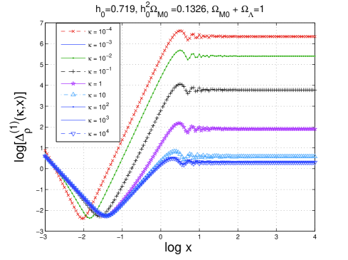
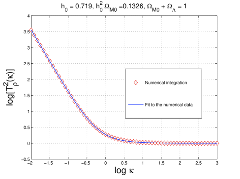
Figure 5: The functions given in Eqs. (6.17) and (6.18) are numerically computed (plot at the left) for different values of $\kappa$ and in the case of the radiation-matter transition. In the plot at the right the transfer function for the spectral energy is illustrated.

Instead of computing the transfer function for the power spectrum it is more direct (and more accurate) to compute directly the spectral energy density and its related transfer function. As previously discussed there can be ambiguities in assigning the energy density because of possible different forms of the energy-momentum pseudo-tensor. In particular in Eqs. (5.46) and (5.48) two different expressions have been proposed on the basis of slightly different physical considerations. The result of the numerical calculation are reported in Fig. 5 in terms of $\Delta^{(1)}_{\rho}(\kappa,x)$ (derived from Eq. (5.46)) and in terms of the transfer function of the spectral energy density (denoted by $T_{\rho}(\kappa)$). The quantities $\Delta^{(1)}_{\rho}(\kappa,x)$ (and, analogously, $\Delta^{(2)}_{\rho}(\kappa,x)$) are defined as

$$\Delta^{(1)}_{\rho}(k,\tau) = \biggl{\{}|g_{k}(\tau)|^{2}+(k^{2}+{\mathcal{H}}^{2})|f_{k}(\tau)|^{2}-{\mathcal{H}}[f_{k}^{*}(\tau)g_{k}(\tau)+f_{k}(\tau)g_{k}^{*}(\tau)]\biggr{\}},$$ (6.17)

$$\Delta^{(2)}_{\rho}(k,\tau) = \biggl{\{}|g_{k}(\tau)|^{2}+(k^{2}-7{\mathcal{H}}^{2})|f_{k}(\tau)|^{2}+3{\mathcal{H}}[f_{k}^{*}(\tau)g_{k}(\tau)+f_{k}(\tau)g_{k}^{*}(\tau)]\biggr{\}}.$$ (6.18)

While Eq. (6.17) follows from Eq. (5.46), Eq. (6.18) follows from Eq. (5.48); Eqs. (6.17)–(6.18) are related to the spectral energy densities in critical units, i.e.

$$\Omega^{(1)}_{\mathrm{GW}}(k,\tau)=\frac{k^{3}}{2\pi^{2}a^{4}\rho_{\mathrm{crit}}}\Delta^{(1)}_{\rho}(k,\tau),\qquad\Omega^{(2)}_{\mathrm{GW}}(k,\tau)=\frac{k^{3}}{2\pi^{2}a^{4}\rho_{\mathrm{crit}}}\Delta^{(2)}_{\rho}(k,\tau).$$ (6.19)

As a function of $x=k\tau$ and $\kappa=k/k_{\mathrm{eq}}$, both $\Delta_{\rho}^{(1)}(\kappa,x)$ and $\Delta_{\rho}^{(2)}(\kappa,x)$ go to a constant value when the relevant modes are evaluated deep inside the Hubble radius. This occurrence allows to introduce the energy transfer function which is defined as:

$$\lim_{x\gg 1}\Delta_{\rho}^{(1,2)}(\kappa,x)\equiv T^{2}_{\rho}(\kappa)\Delta_{\rho}^{(1,2)}(\kappa,x_{\mathrm{i}}),\qquad x_{\mathrm{i}}\ll 1.$$ (6.20)

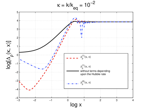
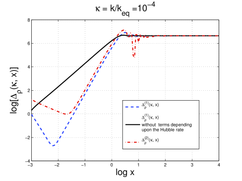
Figure 6: The different definitions of energy-momentum pseudo-tensor (i.e. Eqs. (6.17) and (6.18)) are compared in the determination of the asymptotic value of the energy transfer function.

The specific form of the energy-momentum tensor is immaterial for the determination of $T_{\rho}^{2}(\kappa)$: different forms of the energy-momentum tensor of the relic gravitons will lead to the same result. This aspect can be appreciated by looking at Fig. 6 where $\Delta^{(1,2)}_{\rho}(k,\tau)$ has been reported for $\kappa=10^{-2}$ (plot at the left) and for $\kappa=10^{-4}$ (plot at the right). The dashed and the dot-dashed curves (in both plots) correspond, respectively, to $\Delta_{\rho}^{(1)}(\kappa,x)$ and to $\Delta_{\rho}^{(2)}(\kappa,x)$. The full line, in both plots, corresponds to the combination

$$k^{2}|f_{k}(\tau)|^{2}+|g_{k}(\tau)|^{2}=k(|c_{+}(k)|^{2}+|c_{-}(k)|^{2}),$$ (6.21)

where $c_{\pm}(k)$ are the mixing coefficients which parametrize the solution for the tensor mode functions when the relevant wavelengths are, asymptotically, inside the Hubble radius, i.e.

$$\overline{f}_{k}(\tau)=\frac{1}{\sqrt{2k}}\biggl{[}c_{+}(k)e^{-ik\tau}+c_{-}(k)e^{ik\tau}\biggr{]},\qquad\overline{g}_{k}(\tau)=-i\sqrt{\frac{k}{2}}\biggl{[}c_{+}(k)e^{-ik\tau}-c_{-}(k)e^{ik\tau}\biggr{]}.$$ (6.22)

In Eq. (6.22) $\overline{f}_{k}(\tau)$ and $\overline{g}_{k}(\tau)$ are the solutions to leading order in the limit $k\tau\gg 1$. From Eq. (6.22), $c_{\pm}(k)$ are given by

$$c_{+}(k)=\frac{e^{ik\tau}}{\sqrt{2k}}[k\overline{f}_{k}(\tau)+i\overline{g}_{k}(\tau)],\qquad c_{-}(k)=\frac{e^{-ik\tau}}{\sqrt{2k}}[k\overline{f}_{k}(\tau)-i\overline{g}_{k}(\tau)],$$ (6.23)

Using Eqs. (6.22)–(6.23), Eqs. (6.17)–(6.18) can be directly calculated in the limit $x=k\tau\gg 1$ with the result that

$$\Delta^{(1)}_{\rho}(\kappa,x_{\mathrm{f}})=\Delta^{(2)}_{\rho}(\kappa,x_{\mathrm{f}})=\kappa(|c_{+}(\kappa)|^{2}+|c_{-}(\kappa)|^{2})+{\mathcal{O}}\biggl{(}\frac{1}{x_{\mathrm{f}}}\biggr{)},$$ (6.24)

which proofs that the oscillating contributions are suppressed as $x_{\mathrm{f}}^{-1}$ for $x_{\mathrm{f}}\gg 1$. To get to the results illustrated in Figs. 5 and 6 the evolution equations of the mode functions have been integrated by setting initial conditions deep outside the Hubble radius (i.e. $x=k\tau\ll 1$), by following the corresponding quantities through the Hubble crossing (i.e. $x\simeq 1$) and then, finally, deep inside the Hubble radius (i.e. $x\gg 1$). The integration of the mode functions is most easily performed in terms of $\tilde{f}_{\kappa}(x)=kf_{k}(\tau)$. Using $\tilde{f}_{\kappa}(x)$, $\Delta_{\rho}(\kappa,x)\equiv\Delta^{(1)}_{\rho}(\kappa,x)$ can be written as

$$\Delta_{\rho}(\kappa,x)=|\tilde{f}_{\kappa}(x)|^{2}\biggl{[}1+\biggl{(}\frac{d\ln{a}}{dx}\biggr{)}^{2}\biggr{]}+\left|\frac{d\tilde{f}_{\kappa}}{dx}\right|^{2}-\biggl{(}\frac{d\ln{a}}{dx}\biggr{)}\biggl{[}\biggl{(}\frac{d\tilde{f}_{\kappa}}{dx}\biggr{)}^{*}\tilde{f}_{\kappa}+\biggl{(}\frac{d\tilde{f}_{\kappa}}{dx}\biggr{)}\tilde{f}_{\kappa}^{*}\biggl{]}.$$ (6.25)

In the case of the conventional $\Lambda$CDM scenario, the Universe is suddenly dominated by radiation as soon as inflation ends. Equation (5.4) implies that $F_{k}$ is constant when $k\tau\ll 1$. The initial conditions are fixed by requiring that, at the initial time of the numerical integration,

$$\tilde{f}_{\kappa}(x_{\mathrm{i}})=kf_{k}(\tau_{\mathrm{i}})=ka(\tau)F_{k},\qquad x_{\mathrm{i}}=k\tau_{\mathrm{i}}\ll 1.$$ (6.26)

In Figs. 5 and 5, $x_{\mathrm{i}}=10^{-5}$ even if, for practical reasons, the scale on the horizontal axis has been narrowed. Bearing in mind Eq. (6.15), we can also write, for $x_{\mathrm{i}}\ll 1$,

$$\tilde{f}_{\kappa}(x_{\mathrm{i}})=\frac{2a_{\mathrm{eq}}}{\tau_{1}}F_{k}\,x_{\mathrm{i}},\qquad\left|\frac{d\tilde{f}_{\kappa}}{dx}\right|_{x=x_{\mathrm{i}}}=\frac{2a_{\mathrm{eq}}}{\tau_{1}}F_{k}.$$ (6.27)

To avoid unnecessary complications, the initial condition of the integrations illustrated in Figs. 5 and 6 have been set as $\tilde{f}_{\kappa}(x_{\mathrm{i}})=x_{\mathrm{i}}$, i.e. the initial spectrum has been rescaled. The transfer function, by definition, must always depend only on the dynamics of the transition and not upon the features (e.g slope, amplitude) of the initial power spectrum.

In the plot at the right of Fig. 5, the fit to the energy transfer function is reported with the full (thin) line on top of the diamonds defining the numerical points. The analytical form of the fit can then be written as:

$$T_{\rho}(k/k_{\mathrm{eq}})=\sqrt{1+c_{2}\biggl{(}\frac{k_{\mathrm{eq}}}{k}\biggr{)}+b_{2}\biggl{(}\frac{k_{\mathrm{eq}}}{k}\biggr{)}^{2}},\qquad c_{2}=0.5238,\qquad b_{2}=0.3537.$$ (6.28)

Equation (6.28) permits the accurate evaluation of the spectral energy density of relic gravitons, for instance, in the minimal version of the $\Lambda$CDM paradigm.

Yet another relevant physical situation for the present considerations is the one where the background geometry, after inflation, transits from a stiff epoch to the ordinary radiation-dominated epoch. In the primeval plasma, stiff phases can arise for various reasons. Zeldovich [122] (see also [123]) suggested this possibility in connection with the entropy problem. In [75, 76, 77, 68] it has been suggested that the stiff phase could take place after the inflationary phase with the main purpose of identifying a potential source of high-frequency gravitons. This possibility was also prompted by a possible post-inflationary dominance of a quintessence field.

The simplest consideration leading to the possibility of a post-inflationary phase stiffer than radiation is connected with our extreme ignorance of the thermal history of the Universe after inflation. In a model-independent approach, it is plausible to think that the onset of the radiation-dominance could be delayed. This may happen, in concrete models, for various reasons. One possibility could be that the inflaton field does not decay but rather changes its dynamical nature by acting as quintessence field [78] (see also [126]). In this kind of situations we are the geometry passes from a stiff phase where

$$w_{\mathrm{t}}(\tau) = \frac{p_{\mathrm{t}}}{\rho_{\mathrm{t}}}>\frac{1}{3},$$ (6.29)

$$c^{2}_{\mathrm{st}}(\tau) = \frac{p_{\mathrm{t}}^{\prime}}{\rho_{\mathrm{t}}^{\prime}}=w_{\mathrm{t}}-\frac{w_{\mathrm{t}}^{\prime}}{3{\mathcal{H}}(w_{\mathrm{t}}+1)}=w_{\mathrm{t}}-\frac{1}{3}\frac{d\ln{(w_{\mathrm{t}}+1)}}{d\ln{a}}>\frac{1}{3},$$ (6.30)

to a radiation-dominated phase where $c_{\mathrm{st}}=1/\sqrt{3}$. Note that, according to Eqs. (6.29) and (6.30), $c_{\mathrm{st}}^{2}=w_{\mathrm{t}}$ iff the (total) barotropic index is constant in time. In the limiting case $w_{\mathrm{t}}=1=c_{\mathrm{st}}^{2}$ and the speed of sound coincides with the speed of light. As argued in [124], barotropic indices $w_{\mathrm{t}}>1$ would not be compatible with causality (see, however, [125]). The presence of a suitable stiff phase has been also discussed recently as an effective way of suppressing entropic fluctuations [127] which are observationally constrained by the WMAP 5-yr data.

As in the case of the matter-radiation transition the transfer function only depends upon $\kappa$ which is defined, this time, as $\kappa=k/k_{\mathrm{s}}$, where $k_{\mathrm{s}}=\tau_{\mathrm{s}}^{-1}$ and $\tau_{\mathrm{s}}$ parametrizes the transition time. A simple analytical form of the transition regime is given by

$$a(y)=a_{\mathrm{s}}\sqrt{y^{2}+2y},\qquad y=\frac{\tau}{\tau_{\mathrm{s}}},\qquad\tau_{\mathrm{s}}=\frac{1}{a_{\mathrm{i}}H_{\mathrm{i}}}\sqrt{\frac{\rho_{\mathrm{Si}}}{\rho_{\mathrm{Ri}}}},$$ (6.31)

where, by definition, $\rho_{\mathrm{si}}=\rho_{\mathrm{s}}(\tau_{\mathrm{i}})$ and $\rho_{\mathrm{Ri}}=\rho_{\mathrm{R}}(\tau_{\mathrm{i}})$. Equation (6.31) is a solution of Eqs. (2.2)–(2.4) when the radiation is present together with a stiff component which has, in the case of Eq. (6.31) a sound speed which equals the speed of light. In the limit $y\to 0$ the scale factor expands as $a(y)=\sqrt{2y}$ while, in the opposite limit, $a(y)\simeq y$. In Fig. 7 (plot at the right) $\Delta_{\rho}(\kappa,x)$ is illustrated for different values of $\kappa$. We shall not dwell here (again) about the possible different forms of the energy momentum pseudo-tensor: provided the energy density is evaluated deep inside the Hubble radius the different approaches to the energy density of the relic gravitons give the same result. The transfer function for the spectral energy density is numerically illustrated always in Fig. 7 (plot at the left). The semi-analytical form of the transfer function becomes, this time,

$$T_{\rho}^{2}(k/k_{\mathrm{s}})=1.0+0.204\,\biggl{(}\frac{k}{k_{\mathrm{s}}}\biggr{)}^{1/4}-0.980\,\biggl{(}\frac{k}{k_{\mathrm{s}}}\biggr{)}^{1/2}+3.389\biggl{(}\frac{k}{k_{\mathrm{s}}}\biggr{)}-0.067\,\biggl{(}\frac{k}{k_{\mathrm{s}}}\biggr{)}\ln^{2}{(k/k_{\mathrm{s}})},$$ (6.32)

where $k_{\mathrm{s}}=\tau_{\mathrm{s}}^{-1}$. The value of $k_{\mathrm{s}}$ can be computed in an explicit model but it can also be left as a free parameter. Taking into account that the energy density of the inflaton will be exactly $\rho_{\mathrm{si}}\simeq H_{\mathrm{i}}^{2}\overline{M}_{\mathrm{P}}^{2}$, the value of $k_{\mathrm{s}}$ (as well as the duration of the stiff phase) will be determined, grossly speaking, by $H_{\mathrm{i}}/\overline{M}_{\mathrm{P}}$.

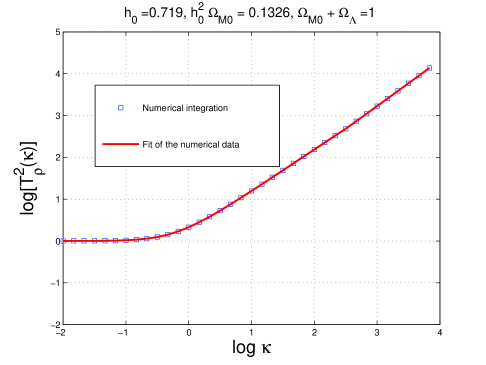
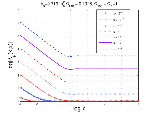
Figure 7: The transition between the stiff phase and the radiation phase is illustrated. The energy transfer function increases with the frequency while the opposite is true for the radiation-matter transition (see Fig. 5 where the analog results have been presented for the matter-radiation transition).

In Fig. (7) (plot at the left) the full line superimposed to the numerical points (illustrated by boxes) is the fit of Eq. (6.32).

6.4 Analytic results for the mixing coefficients

The analytic results for the mixing coefficients are rather useful to obtain the final expression of the various transfer functions. Indeed, defining as $k_{*}$ the typical wavenumber of the transition (e.g. $k_{*}=k_{\mathrm{eq}}$ in the case of the radiation-mattter transition), the slope of the transfer function of the spectral energy density can analytically obtained in the limit $\kappa\gg 1$. This observation helps when we have, for instance, to fit the numerical data points with an analytical expression which will however reproduce the data not only for $\kappa>1$ (as Figs. 5 and 7 clearly show).

For illustration of the method it is practical to consider the transition from a generic accelerated phase to a decelerated stage of expansion. In this situation, by naming the transition point $-\tau_{1}$, the continuous and differentiable form of the scale factors can be written as:

$$a_{\mathrm{i}}(\tau)=\biggl{(}-\frac{\tau}{\tau_{1}}\biggl{)}^{-\beta},\qquad\tau<-\tau_{1},$$ (6.33)

$$a_{\mathrm{s}}(\tau)=\biggl{[}\frac{\beta}{\alpha}\biggl{(}\frac{\tau}{\tau_{1}}+1\biggr{)}+1\biggr{]}^{\alpha},\qquad\tau\geq-\tau_{1},$$ (6.34)

where the scale factors are continuous and differentiable at the transition point which has been generically indicated as $\tau_{1}$. The pump fields of the tensor mode functions turn out to be:

$$\frac{a_{\mathrm{i}}^{\prime\prime}}{a_{\mathrm{i}}}=\frac{\beta(\beta+1)}{\tau^{2}},\qquad\frac{a_{\mathrm{s}}^{\prime\prime}}{a_{\mathrm{s}}}=\frac{\alpha(\alpha-1)}{\biggl{[}\tau+\biggl{(}\frac{\alpha}{\beta}+1\biggr{)}\tau_{1}\biggr{]}^{2}}.$$ (6.35)

The mode functions can then be written as:

$$f_{\mathrm{i}}(\tau) = \frac{{\mathcal{N}}}{\sqrt{2k}}\sqrt{-x}H_{\nu}^{(1)}(-x),\qquad\tau<-\tau_{1},\qquad x=k\tau,$$

$$\tilde{f}_{\mathrm{s}}(\tau) = \frac{\sqrt{y}}{\sqrt{2k}}[{\mathcal{M}}c_{+}(k)H_{\lambda}^{(2)}(y)+{\mathcal{M}}^{*}c_{-}(k)H_{\lambda}^{(1)}(y)],\qquad\tau\geq-\tau_{1},$$ (6.36)

where

$$x=k\tau,\qquad y=k\tau+k\tau_{1}\biggl{(}1+\frac{\alpha}{\beta}\biggr{)}$$

$${\mathcal{N}}=\sqrt{\frac{\pi}{2}}e^{i(\nu+1/2)\pi/2},\qquad{\mathcal{M}}=\sqrt{\frac{\pi}{2}}e^{-i(\lambda+1/2)\pi/2}.$$ (6.37)

The continuity of the tensor mode functions at the transition point

$$f_{\mathrm{i}}(-\tau_{1})=\tilde{f}_{\mathrm{s}}(-\tau_{1}),\qquad g_{\mathrm{i}}(-\tau_{1})=\tilde{g}_{\mathrm{s}}(-\tau_{1}),$$ (6.38)

implies that the mixing coefficients are given by:

$$c_{+}(k) = \frac{i\pi}{8\sqrt{\alpha\beta}}e^{i\pi(\nu+\lambda)/2}\{[\beta(2\lambda+1)+\alpha(2\nu+1)]H_{\nu}^{(1)}(x_{1})H_{\lambda}^{(1)}(y_{1})$$

$$- 2\alpha x_{1}[H_{\lambda}^{(1)}(y_{1})H_{\nu+1}^{(1)}(x_{1})+H_{\nu}^{(1)}(x_{1})H_{\lambda+1}^{(1)}(y_{1})]\},$$

$$c_{-}(k) = \frac{i\pi}{8\sqrt{\alpha\beta}}e^{i\pi(\nu-\lambda)/2}\{[\beta(2\lambda+1)+\alpha(2\nu+1)]H_{\nu}^{(1)}(x_{1})H_{\lambda}^{(2)}(y_{1})$$ (6.39)

$$- 2\alpha x_{1}[H_{\lambda}^{(2)}(y_{1})H_{\nu+1}^{(1)}(x_{1})+H_{\nu}^{(1)}(x_{1})H_{\lambda+1}^{(2)}(y_{1})]\},$$

where, according to the notations previously established, $y_{1}=y(-\tau_{1})=(\alpha/\beta)x_{1}$. The case $\alpha=\beta=1$ corresponds to a transition from the inflationary phase to a radiation-dominated phase. In this case we do know which are the mixing coefficients. The previous expressions give us:

$$c_{-}(k)=\frac{e^{2ix_{1}}}{2x_{1}^{2}},\qquad c_{+}(k)=\biggl{(}1-\frac{1}{2x_{1}^{2}}+\frac{i}{x_{1}}\biggr{)},$$ (6.40)

which clearly agree with previous results [44, 48, 50]. In the case of Eq. (6.40) $|c_{+}(k)|^{2}-|c_{-}(k)|^{2}=1$ and $k^{4}|c_{-}(k)|^{2}$ is exactly scale-invariant. Another interesting situation is the one of the transition from inflation to stiff, i.e. $\beta=1$, $\alpha=1/2$, $y_{1}=x_{1}/2$ which leads to a logarithmic enhancement at small wavenumbers [75, 76]. In this situation the mixing coefficients can be written as:

$$c_{-}(k) = \sqrt{\frac{\pi}{2}}\frac{(i-1)}{4x_{1}^{3/2}}e^{ix_{1}}\biggl{\{}\sqrt{2}e^{-ix_{1}/2}[x_{1}^{2}+6ix_{1}-12]H_{0}^{(2)}(x_{1}/2)$$ (6.41)

$$+ (i+x_{1})[ix_{1}H_{1}^{(2)}(x_{1}/2)-3iH_{0}^{(2)}(x_{1}/2)]\biggr{\}},$$

$$c_{+}(k) = \sqrt{\frac{\pi}{2}}\frac{(i+1)}{4\sqrt{x_{1}}}e^{ix_{1}}\biggl{\{}x_{1}H_{0}^{(1)}(x_{1}/2)+i(i+x_{1})H_{1}^{(1)}(x_{1}/2)\biggr{\}}.$$ (6.42)

The above result can be expanded in for $x_{1}\ll 1$ and the result is:

$$c_{+}(k) = \frac{-0.398(1-\,i)}{{x_{1}}^{\frac{3}{2}}}+\sqrt{x_{1}}\,[\left(0.131+0.338\,i\right)-0.149\left(1-i\right)\ln{x_{1}}]+{\mathcal{O}}(x_{1}^{3/2}),$$ (6.43)

$$c_{-}(k) = \frac{\left(7.031-1.723\,i\right)-16.68\left(1+\,i\right)\,\ln{x_{1}}}{x_{1}^{3/2}}$$ (6.44)

$$+ \sqrt{x_{1}}\,\left[\left(-0.621+0.265\,i\right)+0.282\left(1+i\right)\,\ln{x_{1}}\right]+{\mathcal{O}}({x_{1}}^{3/2}).$$

The logarithms arising in Eqs. (6.43) and (6.44) explain why, in Eq. (6.32), the transfer function of the spectral energy density contains logarithms. In spite of the fact that semi-analytical estimates can pin down the slope of the transfer functions in different intervals, they are insufficient for a faithful account of more realistic situations where the slow-roll corrections are relevant and when other dissipative effects (such as neutrino fee streaming) are taken into account.

6.5 Exponential damping of the mixing coefficients

Consider the case of the $\Lambda$CDM paradigm where the inflationary epoch is almost suddenly followed by the radiation-dominated phase. By denoting the transition time as $\tau_{\mathrm{i}}$, it is plausible to think that all the modes of the field such that $k>a_{\mathrm{i}}H_{\mathrm{i}}\simeq\tau_{\mathrm{i}}^{-1}$ are exponentially suppressed [129, 130]. For the modes $k\tau_{\mathrm{i}}>1$, the pumping action of the gravitational field is practically absent. There will be a given $k$, be it $k_{\mathrm{max}}$, for which $k\simeq\tau_{\mathrm{i}}^{-1}$. The latter wavenumber is, in practice, the maximal $k$ to be amplified and it can be estimated as :

$$k_{\mathrm{max}} = 7.5959\times 10^{25}\,(\pi\epsilon{\mathcal{A}}_{{\mathcal{R}}})^{1/4}\biggl{(}\frac{h_{0}^{2}\Omega_{\mathrm{R}0}}{4.15\times 10^{-5}}\biggr{)}^{1/4}\,\,\mathrm{Mpc}^{-1},$$ (6.45)

$$\nu_{\mathrm{max}} = 1.1745\times 10^{11}\,(\pi\epsilon{\mathcal{A}}_{{\mathcal{R}}})^{1/4}\biggl{(}\frac{h_{0}^{2}\Omega_{\mathrm{R}0}}{4.15\times 10^{-5}}\biggr{)}^{1/4}\,\mathrm{Hz}.$$ (6.46)

Equations (6.45) and (6.46) are derived by assuming that, right after inflation, the radiation-dominated phase takes over. Furthermore, recalling the slow-roll dynamics, $3H^{2}_{\mathrm{i}}\overline{M}_{\mathrm{P}}^{2}\simeq V$ and $V\propto\overline{M}_{\mathrm{P}}^{4}\epsilon\overline{{\mathcal{P}}}_{\mathcal{R}}$. In Eqs. (6.45) and (6.46) ${\mathcal{A}}_{{\mathcal{R}}}$ denotes, as already established, the amplitude of the curvature power spectrum evaluated at the pivot scale.

By taking as typical values of the curvature perturbations at the pivot scale the one endorsed, for instance, by the WMAP 5-yr data alone we will have we will have that Eqs. (6.45) and (6.46) can be written as:

$$k_{\mathrm{max}}=3.5661\times 10^{22}\,\biggl{(}\frac{\epsilon}{0.01}\biggr{)}^{1/4}\biggl{(}\frac{{\mathcal{A}}_{\mathcal{R}}}{2.41\times 10^{-9}}\biggr{)}^{1/4}\biggl{(}\frac{h_{0}^{2}\Omega_{\mathrm{R}0}}{4.15\times 10^{-5}}\biggr{)}^{1/4}\,\,\mathrm{Mpc}^{-1},$$ (6.47)

where the typical values of the slow-roll parameter have been derived by taking into account that, in the absence of running of the tensor spectral index, $r_{\mathrm{T}}=16\epsilon$; since, according to the WMAP 5-yr data alone, $r_{\mathrm{T}}<0.43$, $\epsilon\leq 0.01$.

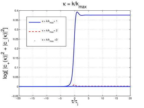
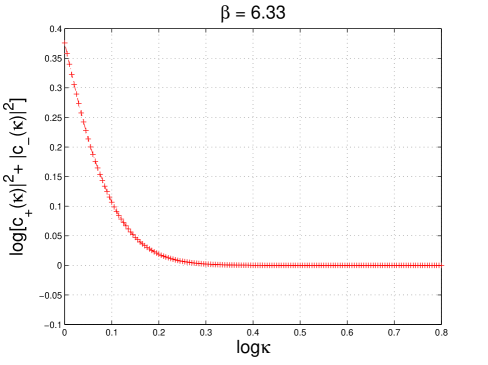
Figure 8: The time evolution of the mixing coefficients is reported at the left (on the horizontal axis the scale is linear). The exponential decay of the mixing coefficients is illustrated in the plot at the right in double logarithmic axes.

For phenomenological purposes it can be also interesting to know what kind of exponential suppression we can expect. From the analysis of various transitions it emerges that the mixing coefficients for $k>k_{\mathrm{max}}$ (or $\nu>\nu_{\mathrm{max}}$) will satisfy

$$|c_{+}(k)|^{2}-|c_{-}|^{2}=1,\qquad|c_{+}(k)|^{2}+|c_{-}(k)|^{2}=e^{-2\beta\frac{k}{k_{\mathrm{max}}}}+1.$$ (6.48)

From Eq. (6.48) we can easily argue that, for $k>k_{\mathrm{max}}$, $|c_{+}(k)|\to 1$ and $|c_{-}(k)|\simeq 2^{-1/2}\exp{[-\beta k/k_{\mathrm{max}}]}$. The point is then to estimate the value of $\beta$ which depends on the nature of the transition regime. Typically, however, $\beta>2$ for sufficiently smooth transitions. To justify this statement it is interesting to consider the following toy model where the scale factor interpolates between a quasi-de Sitter phase and a radiation-dominated phase:

$$a(\tau)=a_{\mathrm{i}}[\tau+\sqrt{\tau^{2}+\tau_{\mathrm{i}}^{2}}].$$ (6.49)

For $\tau\to-\infty$ (i.e. $\tau\ll-\tau_{\mathrm{i}}$) , $a(\tau)\simeq-a_{\mathrm{i}}/\tau$ and the quasi de-Sitter dynamics is recovered. In the opposite limit (i. e. $\tau\gg+\tau_{\mathrm{i}}$), $a(\tau)\simeq a_{\mathrm{i}}\,\tau$ and the radiation dominance is recovered. In Fig. 6 (plot at the left) the exponential damping of the mixing coefficients is numerically illustrated. The curve at the top (full line) illustrates the case $\kappa=1$. The cases $\kappa=2$ and $\kappa=3$ are barely distinguishable at the bottom of the plot. Notice, always in the right plot, the rather narrow range of times which are reported in a linear scale. In the plot at the right the asymptotic values of the mixing coefficients are reported for different values of $\kappa=k/k_{\mathrm{max}}$. By fitting the numerical data with with an equation of the form given in Eq. (6.48), the value of $\beta=6.33$. Different examples can be presented on the same line of the one discussed in Fig. 6. While it is pretty clear that the decay is indeed exponential, the value of $\beta$ may well vary. This can be summarized, for instance, in a rescaling of $k_{\mathrm{max}}$, i.e. by positing, for instance that $k_{\mathrm{max}}\to\tilde{k}_{\mathrm{max}}/\beta$. Thus, the dynamics of the transition can slightly shift the numerical value of the upper cut-off by a numerical factor which depends upon the width of the transition regime.

6.6 Nearly scale-invariant spectra

By using the transfer function for the tensor amplitude, the spectral energy density for frequencies $\nu\gg\nu_{\mathrm{eq}}$ can be simply given by:

$$h_{0}^{2}\Omega_{\mathrm{GW}}(\nu,\tau_{0}) = {\mathcal{N}}_{h}\,\,r_{\mathrm{T}}\,\,\biggl{(}\frac{\nu}{\nu_{\mathrm{p}}}\biggr{)}^{n_{\mathrm{T}}}e^{-2\beta\frac{\nu}{\nu_{\mathrm{max}}}},$$ (6.50)

$${\mathcal{N}}_{h} = 7.992\times 10^{-15}\biggl{(}\frac{h_{0}^{2}\Omega_{\mathrm{M}0}}{0.1326}\biggr{)}^{-2}\biggl{(}\frac{h_{0}^{2}\Omega_{\mathrm{R}0}}{4.15\times 10^{-5}}\biggr{)}\biggl{(}\frac{d_{\mathrm{A}}}{1.4115\times 10^{4}\,\mathrm{Mpc}}\biggr{)}^{-4},$$ (6.51)

where $d_{\mathrm{A}}(z_{*})$ is the (comoving) angular diameter distance to decoupling. In Eqs. (6.50)–(6.51) (as well as in the program used for the numerical calculations) there are two complementary options. The first one is to use the angular diameter distance to decoupling which is directly inferred from the CMB data. For instance, in the case of the 5-yr WMAP data alone, $d_{A}(z_{*})=14115\,\,\mathrm{Mpc}_{-191}^{+188}$. This is the strategy also adopted in other studies [132] (in connection, obviously, with earlier releases of WMAP data). At the same time it is also possible to take the best fit value of the total matter fraction (i.e. $\Omega_{\mathrm{M}0}=0.258$ for the case of the WMAP 5-yr data alone) and compute the comoving angular diameter distance according to the well know expression for spatially flat Universes:

$$d_{\mathrm{A}}(z_{*})=\frac{1}{H_{0}}\int_{0}^{z_{*}}\frac{dz}{\sqrt{\Omega_{\mathrm{M}0}(1+z)^{3}+\Omega_{\Lambda}+\Omega_{\mathrm{R}0}(1+z)^{4}}}=\frac{3.375}{H_{0}}=14072\,\,\mathrm{Mpc},\qquad z_{*}=1090.$$ (6.52)

The latter strategy has been used, for instance, in [131]. The two strategies are compatible and, moreover, this explains why, in Eq. (6.51) the dependence upon $\Omega_{\mathrm{M}0}$ does not cancel. In Eq. (6.50) $n_{\mathrm{T}}$ denotes, as usual, the tensor spectral index which can be also written as

$$n_{\mathrm{T}}=-2\epsilon+\frac{\alpha_{\mathrm{T}}}{2}\ln{(k/k_{\mathrm{p}})},\qquad\alpha_{\mathrm{T}}=\frac{r_{\mathrm{T}}}{8}\biggl{[}(n_{\mathrm{s}}-1)+\frac{r_{\mathrm{T}}}{8}\biggr{]},$$ (6.53)

If $\alpha_{\mathrm{T}}=0$, the standard case is recovered. It should be finally mentioned that, in the limit $\nu\gg\nu_{\mathrm{eq}}$, the oscillating terms have to be appropriately averaged: this is done by setting the terms going as $\cos^{2}{(2\pi\nu\tau_{0})}$ to $1/2$. The latter procedure has been employed, for instance, in the analyses of [132, 38]. In Fig. 9 the transfer function for the spectral energy density (introduced in Eqs. (6.20) and (6.28)) has been consistently employed to estimate the spectral energy density itself and the spectral amplitude. According to Eq. (5.14) the spectral energy density can be written as

$$\Omega_{\mathrm{GW}}(\nu,\tau)=\frac{4\pi^{2}}{3{\mathcal{H}}^{2}}\nu^{3}S_{h}(\nu,\tau),$$ (6.54)

where we used that $k=2\pi\nu$ and that $Ha={\mathcal{H}}$. By making explicit the numerical factors in Eq. (6.54), $S_{h}(\nu,\tau_{0})$ can be expressed in terms of the spectral energy (in critical units)

$$S_{h}(\nu,\tau_{0})=7.981\times 10^{-43}\,\,\biggl{(}\frac{100\,\mathrm{Hz}}{\nu}\biggr{)}^{3}\,\,h_{0}^{2}\Omega_{\mathrm{GW}}(\nu,\tau_{0})\,\,\mathrm{Hz}^{-1},$$ (6.55)

where, we recall, $H_{0}=3.24078\times 10^{-18}\,\,h_{0}\,\,\mathrm{Hz}$.

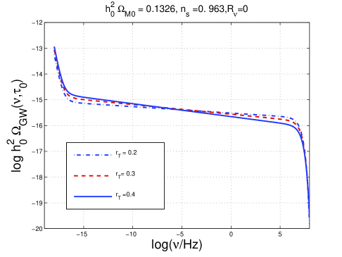
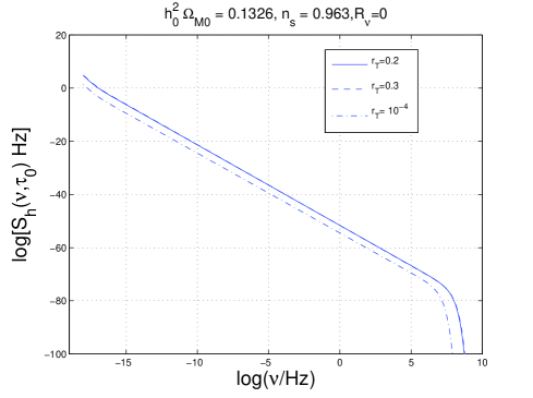
Figure 9: The spectral energy density of the relic gravitons (plot at the left) and the related $S_{h}(\nu,\tau_{0})$ (plot at the right) for different values of $r_{\mathrm{T}}$ and for the same set of fiducial parameters illustrated in Fig. 7.

In Fig. 9 the spectral energy of the relic gravitons as well as $S_{h}(\nu,\tau_{0})$ are reported for different values of $r_{\mathrm{T}}$. The spectra of Fig. 9 have been obtained from the direct integration of the mode functions but can be parametrized, according to Eq. (6.28) as

$$h_{0}^{2}\Omega_{\mathrm{GW}}(\nu,\tau_{0}) = {\mathcal{N}}_{\rho}T^{2}_{\rho}(\nu/\nu_{\mathrm{eq}})r_{\mathrm{T}}\biggl{(}\frac{\nu}{\nu_{\mathrm{p}}}\biggr{)}^{n_{\mathrm{T}}}e^{-2\beta\frac{\nu}{\nu_{\mathrm{max}}}}$$ (6.56)

$${\mathcal{N}}_{\rho} = 4.165\times 10^{-15}\biggl{(}\frac{h_{0}^{2}\Omega_{\mathrm{R}0}}{4.15\times 10^{-5}}\biggr{)}.$$ (6.57)

By comparing Eqs. (6.50)–(6.51) to Eqs. (6.56)–(6.57), the amplitude for $\nu\gg\nu_{\mathrm{eq}}$ differs, roughly, by a factor $2$. This coincidence is not surprising since Eqs. (6.50)–(6.51) have been obtained by averaging over the oscillations (i.e. by replacing cosine squared with $1/2$) and by imposing that $|g_{k}|=k|f_{k}|$. These manipulations are certainly less accurate than the procedure used to derive the transfer function for the spectral energy density.

So far the evolution of the tensor modes has been treated in the absence of anisotropic stress. This approximation is, strictly speaking, unrealistic. Indeed we do know that there are sources of anisotropic stress. After neutrino decoupling, the neutrinos free stream and the effective energy-momentum tensor acquires, to first-order in the amplitude of the plasma fluctuations, an anisotropic stress, i.e.

$$\delta T_{i}^{j}=-\delta p\delta_{i}^{j}+\Pi_{i}^{j},\qquad\partial_{i}\Pi_{j}^{i}=\Pi_{i}^{i}=0.$$ (6.58)

The presence of the anisotropic stress clearly affects the evolution of the tensor modes. To obtain the wanted equation we perturb the Einstein equations to first-order and we get:

$${h_{i}^{j}}^{\prime\prime}+2{\mathcal{H}}{h_{i}^{j}}^{\prime}-\nabla^{2}h_{i}^{j}=-16\pi Ga^{2}\Pi_{i}^{j}.$$ (6.59)

Equation (6.59) reduces to an integro-differential equation which has been analyzed in [36] (see also [37, 38, 39]). The overall effect of collisionless particles is a reduction of the spectral energy density of the relic gravitons. Assuming that the only collisionless species in the thermal history of the Universe are the neutrinos, the amount of suppression can be parametrized by the function

$${\mathcal{F}}(R_{\nu})=1-0.539R_{\nu}+0.134R_{\nu}^{2}$$ (6.60)

where $R_{\nu}$ is the fraction of neutrinos in the radiation plasma. In the case $R_{\nu}=0$ (i.e. in the absence of collisionless patrticles) there is no suppression. If, on the contrary, $R_{\nu}\neq 0$ the suppression can even reach one order of magnitude. In the case $N_{\nu}=3$, $R_{\nu}=0.405$ and the suppression of the spectral energy density is proportional to ${\mathcal{F}}^{2}(0.405)=0.645$. This suppression will be effective for relatively small frequencies which are larger than $\nu_{\mathrm{eq}}$ and smaller than the frequency corresponding to the Hubble radius at the time of big-bang nucleosynthesis, i.e.

$$\nu_{\mathrm{bbn}}=2.252\times 10^{-11}\biggl{(}\frac{g_{\rho}}{10.75}\biggr{)}^{1/4}\biggl{(}\frac{T_{\mathrm{bbn}}}{\,\,\mathrm{MeV}}\biggr{)}\biggl{(}\frac{h_{0}^{2}\Omega_{\mathrm{R}0}}{4.15\times 10^{-5}}\biggr{)}^{1/4}\,\,\mathrm{Hz}.$$ (6.61)

The effect of neutrino free-streaming (as well as all the other late time effects addressed in this subsection) has been taken into account in Fig. 2 (see section 1) but it is absent in Fig. 9. The second effect which has been taken into account in Fig. 2 is the damping associated with the (present) dominance of the dark energy component. Indeed the redshift of $\Lambda$-dominance is simply defined by

$$1+z_{\Lambda}=\biggl{(}\frac{a_{0}}{a_{\Lambda}}\biggr{)}=\biggl{(}\frac{\Omega_{\Lambda}}{\Omega_{\mathrm{M}0}}\biggr{)}^{1/3}.$$ (6.62)

Consider now the mode which will be denoted as $k_{\Lambda}$, i.e. the mode reentering the Hubble radius at $\tau_{\Lambda}$. By definition $k_{\Lambda}=H_{\Lambda}a_{\Lambda}$ must hold. But for $\tau>\tau_{\Lambda}$ is constant, i.e. $H_{\Lambda}\equiv H_{0}$ where $H_{0}$ is the present value of the Hubble rate. Using now Eq. (6.62), it can be easily shown that $k_{\Lambda}=(\Omega_{M0}/\Omega_{\Lambda})^{1/3}k_{\mathrm{H}}$ where $k_{\mathrm{H}}=a_{0}H_{0}$. The frequency interval between $\nu_{\mathrm{H}}$ and $\nu_{\Lambda}$ is rather tiny. Indeed, it turns out that

$$k_{\Lambda}=1.686\times 10^{-4}\,\biggl{(}\frac{h_{0}}{0.719}\biggr{)}\biggl{(}\frac{\Omega_{\mathrm{M}0}}{0.258}\biggr{)}^{1/3}\biggl{(}\frac{\Omega_{\Lambda}}{0.742}\biggr{)}^{1/3}\,\,\mathrm{Mpc}^{-1},$$ (6.63)

$$\nu_{\Lambda}=2.607\times 10^{-19}\biggl{(}\frac{h_{0}}{0.719}\biggr{)}\biggl{(}\frac{\Omega_{\mathrm{M}0}}{0.258}\biggr{)}^{1/3}\biggl{(}\frac{\Omega_{\Lambda}}{0.742}\biggr{)}^{1/3}\,\,\mathrm{Hz}.$$ (6.64)

For the same choice of parameters of Eq. (6.64), $\nu_{\mathrm{H}}=3.708\times 10^{-19}$ Hz which is not so different than $\nu_{\Lambda}=2.607\times 10^{-19}$ Hz. It would therefore seem that this branch of the spectrum could be easily neglected. However, it turns out that the adiabatic damping of the mode function across $\tau_{\Lambda}$ reduces the amplitude of the spectral energy density by a factor $(\Omega_{\mathrm{M}0}/\Omega_{\Lambda})^{2}$. For the typical choice of parameters of Eqs. (6.63) and (6.64) we have that the suppression is of the order of $0.12$. Again this is a tiny number which is, anyway, comparable with the suppression due, for instance, to the neutrino free streaming. This class of effects has been repeatedly in a number of recent papers [137] (see also [145]). The essence of the effect is captured by the following observation. Consider a mode $k$ which reenters before $\tau_{\Lambda}$. The present value of the amplitude $F_{k}(\tau)=f_{k}(\tau)/a(\tau)$ will be adiabatically suppressed since, as repeatedly stressed, in this regime $f_{k}(\tau)$ will simply be plane waves. Consequently, defining as $\tilde{F}_{k_{*}}$ the amplitude at $k_{*}=H_{*}a_{*}$ when the given mode crosses the Hubble radius, we will also have that

$$F_{k}(\tau_{0})=\biggl{(}\frac{a_{k_{*}}}{a_{\Lambda}}\biggr{)}_{\mathrm{mat}}\biggl{(}\frac{a_{\Lambda}}{a_{0}}\biggr{)}_{\Lambda}\tilde{F}_{k_{*}}\equiv\biggl{(}\frac{k}{k_{\mathrm{H}}}\biggr{)}^{-2}\biggl{(}\frac{\Omega_{\mathrm{M}0}}{\Omega_{\Lambda}}\biggr{)}\tilde{F}_{k_{*}},$$ (6.65)

where the subscripts (in the first equality) denote the time range over which the corresponding redshift is computed, i.e. either matter-dominated or $\Lambda$-dominated stages. The second equality follows from the first one by appreciating that $a(k_{*})\simeq\tau_{*}^{2}\simeq k^{-2}$ and by using Eq. (6.62). Equation (6.65) implies, immediately, that the spectral energy density of relic gravitons is corrected in two different fashions. For $\nu<\nu_{\mathrm{H}}$ the frequency dependence will be different and will be proportional to $\Omega_{\mathrm{GW}}(\nu,\tau_{0})\propto(\nu/\nu_{\mathrm{H}})^{n_{\mathrm{T}}-2}(\Omega_{\mathrm{M}0}/\Omega_{\Lambda})^{2}$. Vice versa, in the range $\nu>\nu_{\mathrm{H}}$ the frequency dependence will be exactly the one already computed but, overall, the amplitude will be smaller by a factor $(\Omega_{\mathrm{M}0}/\Omega_{\Lambda})^{2}$. The modification of the frequency dependence is only effective between $0.36$ aHz and $0.26$ aHz: this effect is therefore unimportant and customarily ignored (see, for instance, [132, 137]) for phenomenological purposes. On the other hand, the overall suppression going as $(\Omega_{\mathrm{M}0}/\Omega_{\Lambda})^{2}$ must be taken properly into account on the same footing of other sources of suppression of the spectral energy density. There is, in principle, a third effect which may arise and it has to do with the variation of the effective number of relativistic species. Recall, indeed, that the total energy and the total entropy densities of the plasma can be written as

$$\rho_{\mathrm{t}}=g_{\rho}(T)\frac{\pi^{2}}{30}T^{4},\qquad s_{\mathrm{t}}=g_{\mathrm{s}}(T)\frac{2\pi^{2}}{45}T^{3}.$$ (6.66)

For temperatures much larger than the top quark mass, all the known species of the minimal standard model of particle interactions are in local thermal equilibrium, then $g_{\rho}=g_{\mathrm{s}}=106.75$. Below, $T\simeq 175$ GeV the various species start decoupling, the notion of thermal equilibrium is replaced by the notion of kinetic equilibrium. The time evolution of the number of relativistic degrees of freedom effectively changes the evolution of the Hubble rate. In principle if a given mode $k$ reenters the Hubble radius at a temperature $T_{k}$ the spectral energy density of the relic gravitons is (kinematically) suppressed by a factor which can be estimated as (see, for instance, [137])

$$\biggl{(}\frac{g_{\rho}(T_{k})}{g_{\rho 0}}\biggr{)}\biggl{(}\frac{g_{\mathrm{s}}(T_{k})}{g_{\mathrm{s}0}}\biggr{)}^{-4/3}.$$ (6.67)

At the present time $g_{\rho 0}=3.36$ and $g_{\mathrm{s}0}=3.90$. In general terms the effect parametrized by Eq. (6.67) will cause a frequency-dependent suppression, i.e. a further modulation of the spectral energy density $\Omega_{\mathrm{GW}}(\nu,\tau_{0})$. The maximal suppression one can expect can be obtained by inserting into Eq. (6.67) the largest $g_{\mathrm{s}}$ and $g_{\rho}$. So, in the case of the minimal standard model this would imply that the suppression (on $\Omega_{\mathrm{GW}}(\nu,\tau_{0})$) will be of the order of $0.38$. In popular supersymmetric extensions of the minimal standard models $g_{\rho}$ and $g_{s}$ can be as high as, approximately, $230$. This will bring down the figure given above to $0.29$.

All the three effects estimated in the last part of the present section (i.e. free streaming, dark energy, evolution of relativistic degrees of freedom) have common features. Both in the case of the neutrinos and in the case of the evolution of the relativistic degrees of freedom the potential impact of the effect could be more pronounced. For instance, suppose that, in the early Universe, the particle model has many more degrees of freedom and many more particles which can free stream, at some epoch. At the same time we can say that all the aforementioned effects decrease rather than increasing the spectral energy density. Taken singularly, each of the effects will decrease $\Omega_{\mathrm{GW}}$ by less than one order of magnitude. The net result of the combined effects will then be, roughly, a suppression of $\Omega_{\mathrm{GW}}(\nu,\tau_{0})$ which is of the order of $3\times 10^{-2}$ (for $10^{-16}\,\,\mathrm{Hz}<\nu<10^{-11}\,\mathrm{Hz}$) and of the order of $4\times 10^{-2}$ for $\nu>10^{-11}$Hz. These figures are comparable with the possible inaccuracies stemming from the calculation of the transfer function and, therefore, this is a further motivation, to use the transfer function of the spectral energy density. Finally the late time effects reduce a quantity which is already pretty small, i.e., as computed, $h_{0}^{2}\Omega_{\mathrm{GW}}(\nu,\tau_{0})\simeq 10^{-15}$ for $\nu\gg\nu_{\mathrm{eq}}$.

7 B-modes induced by long wavelength gravitons

In the minimal realization of the $\Lambda$CDM scenario the scalar fluctuations of the geometry induce an E-mode polarization which has been observed and which is now subjected to closer scrutiny [3, 4, 5, 6, 7] The tensor modes of the geometry not only induce an E-mode polarization but also a B-mode polarization. The detected angular power spectra due to the presence of a putative (adiabatic) curvature perturbation are the temperature autocorrelation (TT angular power spectrum) the E-mode autocorrelation (EE angular power spectrum) and their cross correlation (i.e. the TE angular power spectrum). The various angular power spectra of the temperature and polarization observables have been already defined in section 2 (see, in particular, Eqs. (2.48)–(2.49) and discussions therein). Long wavelength gravitons contribute not only to the TT, EE and TE angular power spectra but also to the B-mode autocorrelations, i.e. the BB angular power spectra. The effect of long wavelength gravitons on the temperature and polarization observables can be studied by deriving the evolution equations of the brightness perturbations which are related, in loose terms, to the fluctuations of the Stokes parameters. The tensor nature of the fluctuation defined in Eq. (2.8) plays, in this respect, a decisive role. In particular the following two points should be borne in mind:

• in the case of the scalar modes of the geometry the heat transfer equations have an azimuthal symmetry;

• in the case of the tensor modes the fluctuations of the brightness do depend, both, upon $\mu=\cos{\vartheta}$ as well as upon $\varphi$; this is ultimately, the rationale for the existence of a B-mode polarization.

The heat transfer equations can be schematically written as

$$\biggl{(}\frac{df}{d\tau}\biggr{)}=-\epsilon^{\prime}f+\frac{3\epsilon^{\prime}}{16\pi}\int{\mathcal{M}}(\Omega,\Omega^{\prime})f(\Omega^{\prime})d\Omega^{\prime},$$ (7.1)

where $\epsilon^{\prime}=x_{\mathrm{e}}\tilde{n}_{\mathrm{e}}\sigma_{\mathrm{T}}a$ is the differential optical depth . In the expression for the differential optical depth $\sigma_{\mathrm{T}}=(8/3)\pi r_{0}^{2}$ where $r_{0}=e^{2}/m_{\mathrm{e}}$ is the classical radius of the electron. The (differential) cross section for Compton scattering of polarized photons can be written in terms of $\sigma_{\mathrm{T}}$ and it takes the usual Klein-Nishina form:

$$\frac{d\sigma}{d\Omega}=\frac{3\sigma_{\mathrm{T}}}{32\pi}\biggl{(}\frac{E_{\mathrm{f}}}{E_{\mathrm{i}}}\biggr{)}^{2}\biggl{[}\frac{E_{\mathrm{f}}}{E_{\mathrm{i}}}+\frac{E_{\mathrm{i}}}{E_{\mathrm{f}}}-2+4(\hat{e}\,\cdot\,\hat{e}^{\prime})^{2}\biggr{]},$$ (7.2)

where $\hat{e}$ and $\hat{e}^{\prime}$ are, respectively, the outgoing and ingoing polarizations of the photons; $E_{\mathrm{f}}$ and $E_{\mathrm{i}}$ are, respectively, the energies of the outgoing and of the ingoing photons. In the limit $E_{\mathrm{f}}\simeq E_{\mathrm{i}}$ the differential cross section becomes, as anticipated

$$\frac{d\sigma}{d\Omega}=\frac{3\sigma_{\mathrm{T}}}{8\pi}(\hat{e}\,\cdot\,\hat{e}^{\prime})^{2},$$ (7.3)

The right left side of Eq. (7.1) constitutes the collisionless term while the right hand side is the collisional contribution. At the right-hand side of Eq. (7.3) ${\mathcal{M}}(\Omega,\Omega^{\prime})$ is, in general, a matrix whose dimensionality depends upon the specific problem. As it will be shown ${\mathcal{M}}(\Omega,\Omega^{\prime})$ can be easily computed from Eq. (7.3). In similar terms $f(\Omega)$ should be understood as a column matrix whose components are the various Stokes parameters.

7.1 Collisionless Boltzmann equation for the tensor modes

The collisionless part of the Boltzmann equation can be written as:

$$\frac{df}{d\tau}=\frac{\partial f}{\partial\tau}+\frac{dx^{i}}{d\tau}\frac{\partial f}{\partial x^{i}}+\frac{dq^{i}}{d\tau}\frac{\partial f}{\partial q^{i}},$$ (7.4)

where $q^{i}$ is the comoving three-momentum of the photon. If the tensor fluctuation of the geometry is parametrized as in Eq. (2.8)

$$\delta_{\mathrm{t}}^{(1)}g_{ij}=-a^{2}(\tau)h_{ij}(\vec{x},\tau),$$ (7.5)

then, the right hand side of Eq. (7.4) can be written as

$$\frac{\partial f}{\partial\tau}+\hat{n}^{i}\frac{\partial f}{\partial x^{i}}-\frac{1}{2}\hat{n}^{i}\hat{n}^{j}h_{ij}^{\prime}\frac{\partial f}{\partial q},$$ (7.6)

where the prime denotes a derivation with respect to $\tau$ and where the following identities have been used

$$\frac{\partial f}{\partial q^{i}}=\hat{n}^{i}\frac{\partial f}{\partial q},\qquad\hat{n}^{i}=\frac{dx^{i}}{d\tau}=\frac{q^{i}}{|\vec{q}|},\qquad\frac{dq^{i}}{d\tau}=-\frac{1}{2}h_{ij}^{\prime}q^{j}.$$ (7.7)

In Eq. (7.7) $\hat{n}^{i}$ denotes the direction of the photon momentum. The third identity appearing in Eq. (7.7) stems directly from the definition of comoving three-momentum, i.e.

$$-\delta_{ij}p^{i}p^{j}=g_{ij}P^{i}P^{j},\qquad q^{i}=ap^{i}$$ (7.8)

where $P^{i}$ is a generic spatial component of the canonical momentum obeying

$$g_{\alpha\beta}P^{\alpha}P^{\beta}=0,\qquad P^{\alpha}=\frac{dx^{\alpha}}{d\lambda}.$$ (7.9)

Using Eq. (2.8) the full metric $g_{ij}$ appearing in Eq. (7.8) becomes

$$g_{ij}=-a^{2}(\tau)\delta_{ij}+\delta_{\mathrm{t}}^{(1)}g_{ij}\equiv-a^{2}(\tau)(\delta_{ij}+h_{ij}).$$ (7.10)

Consequently the comoving three-momentum $q^{i}$ and its conformal time derivative can be expressed as:

$$q^{i}=a^{2}\biggl{(}\delta^{i}_{j}+\frac{1}{2}h_{j}^{i}\biggr{)}\,P^{j},$$ (7.11)

$$\frac{dq^{i}}{d\tau}=\biggl{[}2a^{2}{\mathcal{H}}\biggl{(}\delta_{j}^{i}+\frac{1}{2}h_{j}^{i}\biggr{)}P^{j}+\frac{a^{2}}{2}{h_{j}^{i}}^{\prime}P^{j}+a^{2}\biggl{(}\delta_{j}^{i}+\frac{1}{2}h_{j}^{i}\biggr{)}\frac{dP^{j}}{d\tau}\biggr{]}.$$ (7.12)

To obtain an explicit expression for $dq^{i}/d\tau$ the conformal time derivative of the canonical momentum should be made explicit by using the geodesic equation, i.e.

$$\frac{dP^{i}}{d\tau}+\Gamma^{i}_{\mu\nu}\frac{P^{\mu}P^{\nu}}{P^{0}}=0,\qquad P^{\mu}=\frac{dx^{\mu}}{d\lambda}=P^{0}\frac{dx^{i}}{d\tau}.$$ (7.13)

To first order in the tensor fluctuations of the geometry the Christoffel connection will then lead to the following expression:

$$\Gamma_{j0}^{i}=\biggl{(}{\mathcal{H}}\delta_{j}^{i}+\frac{1}{2}{h_{j}^{i}}^{\prime}\biggr{)}.$$ (7.14)

Using Eq. (7.14) into Eqs. (7.12) and (7.13), the third identity reported in Eq. (7.7) is quickly recovered. Depending upon the problem at hand the collisionless part of the Boltzmann equation can be written in different (but equivalent) forms. Equation (2.9) allows to write $h_{ij}^{\prime}$ in terms of the two polarizations:

$$h_{ij}^{\prime}=\sum_{\lambda}h_{(\lambda)}^{\prime}\epsilon^{(\lambda)}_{ij}\equiv h^{\prime}_{\oplus}\epsilon_{ij}^{\oplus}+h_{\otimes}^{\prime}\epsilon_{ij}^{\otimes}.$$ (7.15)

Using Eqs. (7.7) and (7.15), Eq. (7.6) can be written, in Fourier space, as

$$\frac{\partial f}{\partial\tau}+ik\mu f-\frac{1}{2}\frac{\partial f}{\partial\ln{q}}\biggl{\{}[(\hat{n}\cdot\hat{a})^{2}-(\hat{n}\cdot\hat{b})^{2}]h_{\oplus}^{\prime}+2(\hat{n}\cdot\hat{a})(\hat{n}\cdot\hat{b})h_{\otimes}^{\prime}\biggr{\}}={\mathcal{C}}_{\mathrm{coll}},$$ (7.16)

where ${\mathcal{C}}_{\mathrm{coll}}$ denotes, for completeness, the collisional part of the Boltzmann equation; $\mu=\hat{k}\cdot\hat{n}$ is the projection of the photon momentum on the direction of the Fourier mode. If the direction of propagation of the gravitational wave coincides with the third (Cartesian) component, i.e. $\hat{k}=\hat{z}$. It is then easy to see that the unit vectors $\hat{a}$ and $\hat{b}$ must be directed, respectively, along the $\hat{x}$ and $\hat{y}$ Cartesian directions. This particular choice of the coordinate system implies then

$$(\hat{n}\cdot\hat{a})^{2}-(\hat{n}\cdot\hat{b})^{2}=n_{x}^{2}-n_{y}^{2}=(1-\mu^{2})\cos{2\varphi},$$ (7.17)

$$2(\hat{n}\cdot\hat{a})(\hat{n}\cdot\hat{b})=2n_{x}n_{y}=(1-\mu^{2})\sin{2\varphi}.$$ (7.18)

Equations (7.17) and (7.18) are not symmetric for $\varphi\to-\varphi$: while Eq. (7.17) is left unchanged, Eq. (7.18) acquires a minus sign. Conversely, the evolution equations of the scalar modes of the geometry are symmetric for $\varphi\to-\varphi$.

7.2 Azimuthal structure of the collisional contribution

The differential cross section of Eq. (7.3) depends upon $\hat{e}$ and $\hat{e}^{\prime}$ which are, respectively, the polarizations of the outgoing and of the ingoing photons. If $\hat{k}$ coincides with the radial direction $\hat{e}$ and $\hat{e}^{\prime}$ can be written, respectively, as

$$\hat{k}=(\sin{\vartheta}\,\cos{\varphi},\sin{\vartheta}\,\sin{\varphi},\,\cos{\vartheta}),$$

$$\hat{e}_{x}=(\cos{\vartheta}\,\cos{\varphi},\,\cos{\vartheta}\,\sin{\varphi},\,-\sin{\vartheta}),\qquad\hat{e}_{y}=(\sin{\varphi},\,-\cos{\varphi},\,0),$$ (7.19)

$$\hat{k}^{\prime}=(\sin{\vartheta^{\prime}}\,\cos{\varphi^{\prime}},\,\sin{\vartheta^{\prime}}\,\sin{\varphi^{\prime}},\,\cos{\vartheta^{\prime}}),$$

$$\hat{e}_{x}^{\prime}=(\cos{\vartheta^{\prime}}\,\cos{\varphi^{\prime}},\,\cos{\vartheta^{\prime}}\,\sin{\varphi^{\prime}},\,-\sin{\vartheta^{\prime}}),\qquad\hat{e}_{y}^{\prime}=(\sin{\varphi^{\prime}},\,-\cos{\varphi^{\prime}},\,0).$$ (7.20)

In Eqs. (7.19) and (7.20) the components of $\hat{e}$ and $\hat{e}^{\prime}$ have been identified with the $\hat{x}$ and $\hat{y}$ directions. This is just to guide the intuition since the components of $\hat{e}$ and $\hat{e}^{\prime}$ should only be orthogonal to each others and orthogonal to the direction of propagation. Furthermore notice that, in the case $\vartheta^{\prime}=\varphi^{\prime}=0$,

$$\hat{k}^{\prime}=(0,\,0,\,1),\qquad\hat{e}_{x}^{\prime}=(1,\,0,\,0),\qquad\hat{e}_{y}^{\prime}=(0,\,-1,\,0).$$ (7.21)

Under the transformation $\varphi\to-\varphi$ and $\varphi^{\prime}\to-\varphi^{\prime}$, Eqs. (7.19) and (7.20) lead to another valid choice of orthogonal frame. The intensity and the polarization of the (outgoing) radiation field will be given, respectively, as

$$I(\tau,\vartheta,\varphi)={\mathcal{I}}_{x}(\tau,\vartheta,\varphi)+{\mathcal{I}}_{y}(\tau,\vartheta,\varphi),\qquad Q(\tau,\vartheta,\varphi)={\mathcal{I}}_{x}(\tau,\vartheta,\varphi)-{\mathcal{I}}_{y}(\tau,\vartheta,\varphi),$$ (7.22)

Since $Q$ and $U$ are not invariant for a rotation in the polarization plane and as soon as $Q$ is generated also $U$ follows (see, e.g., Eqs. (2.37) and discussion therein). For pedagogical purposes, it is useful to consider, as a warm-up the simplification provided by Eq. (7.22). Consider the case where the ingoing polarization is fixed (e. g. $\vartheta^{\prime}=\varphi^{\prime}=0$); suppose also, for sake of simplicity, that the dependence of the Stokes parameters upon the conformal time coordinate is trivial. Using Eq. (7.3) the outgoing Stokes parameters are given by

$${\mathcal{I}}_{x}(\vartheta,\varphi)=\frac{3\epsilon^{\prime}}{8\pi}\biggl{[}(\hat{e}_{x}\,\hat{e}_{x}^{\prime})^{2}{\mathcal{I}}_{x}^{\prime}+(\hat{e}_{x}\,\hat{e}_{y}^{\prime})^{2}{\mathcal{I}}_{y}^{\prime}\biggr{]},$$ (7.23)

$${\mathcal{I}}_{y}(\tau,\vartheta,\varphi)=\frac{3\epsilon^{\prime}}{8\pi}\biggl{[}(\hat{e}_{y}\,\hat{e}_{x}^{\prime})^{2}{\mathcal{I}}_{x}^{\prime}+(\hat{e}_{y}\,\hat{e}_{y}^{\prime})^{2}{\mathcal{I}}_{y}^{\prime}\biggr{]}.$$ (7.24)

In the generic situation the ingoing Stokes parameters do depend upon $\varphi^{\prime}$ and $\vartheta^{\prime}$ and, therefore, the outgoing Stokes parameters are

$${\mathcal{I}}_{x}(\vartheta,\varphi)=\frac{3\epsilon^{\prime}}{8\pi}\,\int d\Omega^{\prime}\biggl{[}(\hat{e}_{x}\,\hat{e}_{x}^{\prime})^{2}{\mathcal{I}}_{x}^{\prime}(\vartheta^{\prime},\varphi^{\prime})+(\hat{e}_{x}\,\hat{e}_{y}^{\prime})^{2}{\mathcal{I}}_{y}^{\prime}(\vartheta^{\prime},\varphi^{\prime})\biggr{]},$$ (7.25)

$${\mathcal{I}}_{y}(\vartheta,\varphi)=\frac{3\epsilon^{\prime}}{8\pi}\,\int d\Omega^{\prime}\biggl{[}(\hat{e}_{y}\,\hat{e}_{x}^{\prime})^{2}{\mathcal{I}}_{x}^{\prime}(\vartheta^{\prime},\varphi^{\prime})+(\hat{e}_{y}\,\hat{e}_{y}^{\prime})^{2}{\mathcal{I}}_{y}^{\prime}(\vartheta^{\prime},\varphi^{\prime})\biggr{]}.$$ (7.26)

From the definitions of $\hat{e}$ and $\hat{e}^{\prime}$, simple trigonometric identities lead to the following expressions for the four products appearing in Eqs. (7.25) and (7.26):

$$(\hat{e}_{x}\,\hat{e}_{x}^{\prime})=\mu\,\mu^{\prime}\cos{(\varphi^{\prime}-\varphi)}+\sqrt{1-\mu^{2}}\,\sqrt{1-{\mu^{\prime}}^{2}},\qquad(\hat{e}_{x}\,\hat{e}_{y}^{\prime})=\mu\,\sin{(\varphi^{\prime}-\varphi)},$$ (7.27)

$$(\hat{e}_{y}\,\hat{e}_{x}^{\prime})=-\mu^{\prime}\,\sin{(\varphi^{\prime}-\varphi)},\qquad(\hat{e}_{y}\,\hat{e}_{y}^{\prime})=\cos{(\varphi^{\prime}-\varphi)}.$$ (7.28)

As already mentioned, in Eqs. (7.27) and (7.28) the notations

$$\mu=\cos{\vartheta},\qquad\mu^{\prime}=\cos{\vartheta^{\prime}},\qquad\sin{\vartheta}=\sqrt{1-\mu^{2}},\qquad\sin{\vartheta^{\prime}}=\sqrt{1-{\mu^{\prime}}^{2}},$$ (7.29)

have been used. The results of Eqs. (7.25)–(7.26) and of Eqs. (7.27)–(7.28) allow for an explicit evaluation of the the collisional part of the Boltzmann equation which can be written, component by component, in the simplified case where $f(\tau,\vartheta,\varphi)$ has only two components which can be identified with the intensities of the radiation field along the $x$ and $y$ axes

$$f(\tau,\vartheta,\varphi)=({\mathcal{I}}_{x}(\tau,\vartheta,\varphi),\,{\mathcal{I}}_{y}(\tau,\vartheta,\varphi)).$$ (7.30)

The result is:

$$\frac{d{\mathcal{I}}_{x}}{d\tau}=-\epsilon^{\prime}{\mathcal{I}}_{x}$$

$$+\frac{3\epsilon^{\prime}}{16\pi}\int_{-1}^{1}d\mu^{\prime}\int_{0}^{2\pi}d\varphi^{\prime}[{\mathcal{M}}_{11}(\mu,\mu^{\prime},\varphi,\varphi^{\prime}){\mathcal{I}}_{x}^{\prime}(\tau,\mu^{\prime},\varphi^{\prime})+{\mathcal{M}}_{12}(\mu,\mu^{\prime},\varphi,\varphi^{\prime}){\mathcal{I}}_{y}^{\prime}(\tau,\mu^{\prime},\varphi^{\prime})]$$ (7.31)

$$\frac{d{\mathcal{I}}_{y}}{d\tau}=-\epsilon^{\prime}{\mathcal{I}}_{y}$$

$$+\frac{3\epsilon^{\prime}}{16\pi}\int_{-1}^{1}d\mu^{\prime}\int_{0}^{2\pi}d\varphi^{\prime}[{\mathcal{M}}_{21}(\mu,\mu^{\prime},\varphi,\varphi^{\prime}){\mathcal{I}}_{x}^{\prime}(\tau,\mu^{\prime},\varphi^{\prime})+{\mathcal{M}}_{22}(\mu,\mu^{\prime},\varphi,\varphi^{\prime}){\mathcal{I}}_{y}^{\prime}(\tau,\mu^{\prime},\varphi^{\prime})],$$ (7.32)

where, by definition,

$${\mathcal{M}}_{11}(\mu,\mu^{\prime},\varphi,\varphi^{\prime}) = 2(\hat{e}_{x}\,\hat{e}_{x}^{\prime})^{2}=\mu^{2}\mu^{\prime 2}+2(1-\mu^{2})(1-\mu^{\prime 2})+\mu^{2}\mu^{\prime 2}\cos{2(\varphi^{\prime}-\varphi)}$$ (7.33)

$$+ 4\mu\,\mu^{\prime}\sqrt{1-\mu^{2}}\sqrt{1-{\mu^{\prime}}^{2}}\cos{(\varphi^{\prime}-\varphi)},$$

$${\mathcal{M}}_{12}(\mu,\mu^{\prime},\varphi,\varphi^{\prime}) = 2(\hat{e}_{x}\,\hat{e}_{y}^{\prime})^{2}=\mu^{2}[1-\cos{2(\varphi^{\prime}-\varphi)}],$$ (7.34)

$${\mathcal{M}}_{21}(\mu,\mu^{\prime},\varphi,\varphi^{\prime}) = 2(\hat{e}_{y}\,\hat{e}_{x}^{\prime})^{2}=\mu^{\prime 2}-\mu^{\prime 2}\cos{2(\varphi^{\prime}-\varphi)},$$ (7.35)

$${\mathcal{M}}_{22}(\mu,\mu^{\prime},\varphi,\varphi^{\prime}) = 2(\hat{e}_{y}\,\hat{e}_{y}^{\prime})^{2}=1+\cos{2(\varphi^{\prime}-\varphi)}.$$ (7.36)

The second equality appearing in Eqs. (7.33)–(7.36) follows immediately from Eqs. (7.27) and (7.28). If ${\mathcal{I}}_{x}^{\prime}$ and ${\mathcal{I}}_{y}^{\prime}$ do not depend on $\varphi^{\prime}$, Eqs. (7.31) and (7.32) can be simplified by integrating explicitly upon $\varphi^{\prime}$:

$$\frac{d{\mathcal{I}}_{x}}{d\tau}=-\epsilon^{\prime}{\mathcal{I}}_{x}+\frac{3\epsilon^{\prime}}{8}\int_{-1}^{1}d\mu^{\prime}\{[\mu^{2}\mu^{\prime 2}+2(1-\mu^{2})(1-\mu^{\prime 2})]{\mathcal{I}}_{x}^{\prime}(\tau,\mu^{\prime})+\mu^{2}{\mathcal{I}}_{y}^{\prime}(\tau,\mu^{\prime})\},$$ (7.37)

$$\frac{d{\mathcal{I}}_{y}}{d\tau}=-\epsilon^{\prime}{\mathcal{I}}_{y}+\frac{3\epsilon^{\prime}}{8}\int_{-1}^{1}d\mu^{\prime}\{[\mu^{\prime 2}{\mathcal{I}}_{x}^{\prime}(\tau,\mu^{\prime})+{\mathcal{I}}_{y}^{\prime}(\tau,\mu^{\prime})\}.$$ (7.38)

Equations (7.37) and (7.38) is just a useful warm-up in view of the realistic situation where:

• the components of $f(\vartheta,\varphi)$ are not $2$ but $3$, i.e. ${\mathcal{I}}_{x}(\vartheta,\varphi)$ and ${\mathcal{I}}_{y}(\vartheta,\varphi)$ are supplemented by $U(\vartheta,\varphi)$;

• all the $3$ components of $f(\vartheta,\varphi)$ do depend upon $\varphi$; in the analog of Eqs. (7.37) and (7.38) on top of the integration over $\mu^{\prime}$ an integration over $\varphi^{\prime}$ will appear.

Since $f(\vartheta,\varphi)$ has now three components

$$f(\tau,\vartheta,\varphi)=({\mathcal{I}}_{x}(\tau,\vartheta,\varphi),\,{\mathcal{I}}_{y}(\tau,\vartheta,\varphi),\,U(\tau,\vartheta,\varphi)).$$ (7.39)

${\mathcal{M}}(\Omega,\Omega^{\prime})$ will be a $3\times 3$ matrix whose entries can be computed in full analogy with what has been already done in Eqs. (7.33)–(7.36). In general terms, the ingoing electric field can be expressed as

$$\vec{E}^{\prime}(\tau,\vartheta^{\prime},\varphi^{\prime})=E_{x}^{\prime}(\tau,\vartheta^{\prime},\varphi^{\prime})\,\hat{e}_{x}^{\prime}+E_{y}^{\prime}(\tau,\vartheta^{\prime},\varphi^{\prime})\,\hat{e}_{y}^{\prime},$$ (7.40)

implying that the outgoing Stokes parameters can be written as

$${\mathcal{I}}_{x}(\tau,\vartheta,\varphi)=\frac{3\epsilon^{\prime}}{8\pi}\int d\Omega^{\prime}(\hat{e}_{x}\,\cdot\vec{E}\,^{\prime})^{2},$$ (7.41)

$${\mathcal{I}}_{y}(\tau,\vartheta,\varphi)=\frac{3\epsilon^{\prime}}{8\pi}\int d\Omega^{\prime}(\hat{e}_{y}\,\cdot\vec{E}\,^{\prime})^{2},$$ (7.42)

$$U(\tau,\vartheta,\varphi)=\frac{3\epsilon^{\prime}}{8\pi}\int d\Omega^{\prime}[2(\hat{e}_{x}\cdot\vec{E}\,^{\prime})(\hat{e}_{y}\cdot\vec{E}\,^{\prime})].$$ (7.43)

where, for the moment, the collisionless part of the Boltzmann equation has been neglected. Inserting Eq. (7.40) into Eqs. (7.41)–(7.43) the explicit form of ${\mathcal{M}}(\Omega,\Omega^{\prime})$ since the Stokes parameters of the ingoing radiation field are nothing but

$${\mathcal{I}}_{x}^{\prime}=E_{x}^{\prime 2},\qquad{\mathcal{I}}_{y}^{\prime}=E_{y}^{\prime 2},\qquad U^{\prime}=2\,E_{x}^{\prime}E_{y}^{\prime}.$$ (7.44)

The terms ${\mathcal{M}}_{11}$, ${\mathcal{M}}_{12}$, ${\mathcal{M}}_{21}$, ${\mathcal{M}}_{22}$ will be exactly the ones already evaluated in Eqs. (7.33)–(7.36). The remaining entries are found to be

$${\mathcal{M}}_{13}(\mu,\mu^{\prime},\varphi,\varphi^{\prime}) = 2\,(\hat{e}_{x}^{\prime}\,\hat{e}_{x})(\hat{e}_{x}\,\hat{e}_{y}^{\prime})=\mu^{2}\mu^{\prime}\sin{2(\varphi^{\prime}-\varphi)}$$ (7.45)

$$+ 2\mu\sqrt{1-\mu^{2}}\sqrt{1-\mu^{\prime 2}}\sin{(\varphi^{\prime}-\varphi)},$$

$${\mathcal{M}}_{23}(\mu,\mu^{\prime},\varphi,\varphi^{\prime}) = 2\,(\hat{e}_{x}^{\prime}\,\hat{e}_{y})(\hat{e}_{y}\,\hat{e}_{y}^{\prime})=-\mu^{\prime}\sin{2(\varphi^{\prime}-\varphi)},$$ (7.46)

$${\mathcal{M}}_{31}(\mu,\mu^{\prime},\varphi,\varphi^{\prime}) = 4(\hat{e}_{x}^{\prime}\,\hat{e}_{x})(\hat{e}_{y}\,\hat{e}_{x}^{\prime})=-2\mu^{\prime 2}\mu\sin{2(\varphi^{\prime}-\varphi)}$$ (7.47)

$$- 4\mu^{\prime}\sqrt{1-\mu^{2}}\sqrt{1-\mu^{\prime 2}}\sin{(\varphi^{\prime}-\varphi)},$$

$${\mathcal{M}}_{32}(\mu,\mu^{\prime},\varphi,\varphi^{\prime}) = 4(\hat{e}_{x}\,\hat{e}_{y}^{\prime})(\hat{e}_{y}\,\hat{e}_{y}^{\prime})=2\mu\sin{2(\varphi^{\prime}-\varphi)},$$ (7.48)

$${\mathcal{M}}_{33}(\mu,\mu^{\prime},\varphi,\varphi^{\prime}) = 2(\hat{e}_{x}\,\hat{e}_{x}^{\prime})(\hat{e}_{y}\,\hat{e}_{y}^{\prime})+2(\hat{e}_{x}\,\hat{e}_{y}^{\prime})(\hat{e}_{y}\,\hat{e}_{x}^{\prime})=2\mu\mu^{\prime}\cos{2(\varphi^{\prime}-\varphi)}$$ (7.49)

$$+ 2\sqrt{1-\mu^{2}}\sqrt{1-\mu^{\prime 2}}\cos{(\varphi^{\prime}-\varphi)}.$$

As in Eqs. (7.33)–(7.36), the second equality in each of Eqs. (7.45)–(7.49) follows immediately from Eqs. (7.27) and (7.28). A final remark on the symmetry properties of the various entries of ${\mathcal{M}}(\Omega,\Omega^{\prime})$ is in order:

• ${\mathcal{M}}_{11}$, ${\mathcal{M}}_{12}$, ${\mathcal{M}}_{21}$, ${\mathcal{M}}_{22}$ and ${\mathcal{M}}_{33}$ are all symmetric under the simultaneous transformation $\varphi\to-\varphi$ and $\varphi^{\prime}\to-\varphi^{\prime}$;

• for the same transformation, the remaining entries flip their respective sign.

7.3 Different parametrizations of the full equation

The phase space distribution obeying the collisionless part of the Boltzmann equation (see, e. g., Eq. (7.16)) does depend upon $k=|\vec{k}|$ (i.e. the Fourier mode). In the previous subsection the dependence upon $k$ has been suppressed (for sake of simplicity) since all the aforementioned considerations could be separately repeated for each Fourier mode. Similarly, from Eq. (7.16), it is clear that the phase-space distribution does depend not only upon $\hat{n}$ (i.e. the direction of the photon) but also upon its comoving three-momentum. The phase space distribution consists of $3$ independent functions whose dependence can be written, in Fourier space, as:

$$f(k,\tau,\mu,\varphi,q)=[{\mathcal{I}}_{x}(k,\tau,\mu,\varphi,q),{\mathcal{I}}_{y}(k,\tau,\mu,\varphi,q),U(k,\tau,\mu,\varphi,q)].$$ (7.50)

As already discussed it is more handy to use directly $\mu=\cos{\vartheta}$ as independent variable. The full Boltzmann equation can then be solved by iteration around the equilibrium configuration provided by the Bose-Einstein distribution $f_{0}(q)$; this means that the $3$ components of $f(\tau,\mu,\varphi)$ can be written as:

$${\mathcal{I}}_{x}(k,\tau,\mu,\varphi,q)=f_{0}(q)[1+\overline{{\mathcal{I}}}_{x}(k,\tau,\mu,\varphi)],$$ (7.51)

$${\mathcal{I}}_{y}(k,\tau,\mu,\varphi,q)=f_{0}(q)[1+\overline{{\mathcal{I}}}_{y}(k,\tau,\mu,\varphi)],$$ (7.52)

$$U(k,\tau,\mu,\varphi,q)=f_{0}(q)\overline{U}(k,\tau,\mu,\varphi).$$ (7.53)

The solution of the problem will then require the determination of $\overline{{\mathcal{I}}}_{x}(k,\tau,\mu,\varphi)$, $\overline{{\mathcal{I}}}_{y}(k,\tau,\mu,\varphi)$ and $\overline{U}(k,\tau,\mu,\varphi)$. The form of the final solution for $\overline{{\mathcal{I}}}_{x}(k,\tau,\mu,\varphi)$, $\overline{{\mathcal{I}}}_{y}(k,\tau,\mu,\varphi)$ and $\overline{U}(k,\tau,\mu,\varphi)$ will depend upon the polarization of the relic graviton. This aspect cal be appreciated by looking at the collisionless part of the full Boltzmann equation, i.e. Eq. (7.16). Consider, for sake of concreteness, the case of the $\oplus$ polarization. Inserting Eq. (7.50) into Eq. (7.16) and using the perturbative scheme of Eqs. (7.51)–(7.53), the three independent components of the Boltzmann equation become:

$$\frac{\partial\overline{{\mathcal{I}}}_{x}}{\partial\tau}+(ik\mu+\epsilon^{\prime})\overline{{\mathcal{I}}}_{x}-\frac{1}{2}\frac{\partial h_{\oplus}}{\partial\tau}\cos{2\varphi}(1-\mu^{2})\frac{\partial\ln{f_{0}}}{\partial\ln{q}}={\mathcal{C}}_{x}(k,\tau,\mu,\varphi),$$ (7.54)

$$\frac{\partial\overline{{\mathcal{I}}}_{y}}{\partial\tau}+(ik\mu+\epsilon^{\prime})\overline{{\mathcal{I}}}_{y}-\frac{1}{2}\frac{\partial h_{\oplus}}{\partial\tau}\cos{2\varphi}(1-\mu^{2})\frac{\partial\ln{f_{0}}}{\partial\ln{q}}={\mathcal{C}}_{y}(k,\tau,\mu,\varphi),$$ (7.55)

$$\frac{\partial\overline{U}}{\partial\tau}+(ik\mu+\epsilon^{\prime})\overline{U}={\mathcal{C}}_{U}(k,\tau,\mu,\varphi),$$ (7.56)

where, for convenience, the collision terms ${\mathcal{C}}_{x}(k,\tau,\mu,\varphi)$, ${\mathcal{C}}_{y}(k,\tau,\mu,\varphi)$ and ${\mathcal{C}}_{U}(k,\tau,\mu,\varphi)$ have been expressed as:

$${\mathcal{C}}_{x}(k,\tau,\mu,\varphi)=\frac{3\epsilon^{\prime}}{16\pi}\int d\mu^{\prime}d\varphi^{\prime}[{\mathcal{M}}_{11}(\mu,\mu^{\prime},\varphi,\varphi^{\prime})\overline{{\mathcal{I}}}_{x}(k,\tau,\mu^{\prime},\varphi^{\prime})+{\mathcal{M}}_{12}(\mu,\mu^{\prime},\varphi,\varphi^{\prime})\overline{{\mathcal{I}}}_{y}(k,\tau,\mu^{\prime},\varphi^{\prime})$$

$$+{\mathcal{M}}_{13}(\mu,\mu^{\prime},\varphi,\varphi^{\prime})\overline{U}(k,\tau,\mu^{\prime},\varphi^{\prime})],$$ (7.57)

$${\mathcal{C}}_{y}(k,\tau,\mu,\varphi)=\frac{3\epsilon^{\prime}}{16\pi}\int d\mu^{\prime}d\varphi^{\prime}[{\mathcal{M}}_{21}(\mu,\mu^{\prime},\varphi,\varphi^{\prime})\overline{{\mathcal{I}}}_{x}(k,\tau,\mu^{\prime},\varphi^{\prime})+{\mathcal{M}}_{22}(\mu,\mu^{\prime},\varphi,\varphi^{\prime})\overline{{\mathcal{I}}}_{y}(k,\tau,\mu^{\prime},\varphi^{\prime})$$

$$+{\mathcal{M}}_{23}(\mu,\mu^{\prime},\varphi,\varphi^{\prime})\overline{U}(k,\tau,\mu^{\prime},\varphi^{\prime})],$$ (7.58)

$${\mathcal{C}}_{U}(k,\tau,\mu,\varphi)=\frac{3\epsilon^{\prime}}{16\pi}\int d\mu^{\prime}d\varphi^{\prime}[{\mathcal{M}}_{31}(\mu,\mu^{\prime},\varphi,\varphi^{\prime})\overline{{\mathcal{I}}}_{x}(k,\tau,\mu^{\prime},\varphi^{\prime})+{\mathcal{M}}_{32}(\mu,\mu^{\prime},\varphi,\varphi^{\prime})\overline{{\mathcal{I}}}_{y}(k,\tau,\mu^{\prime},\varphi^{\prime})$$

$$+{\mathcal{M}}_{33}(\mu,\mu^{\prime},\varphi,\varphi^{\prime})\overline{U}(k,\tau,\mu^{\prime},\varphi^{\prime})].$$ (7.59)

In the case of the $\otimes$ polarization Eqs. (7.54)–(7.56) lead to a similar result where, however, the relevant part of the collisionless contribution is different and it is given by the replacement

$$\frac{1}{2}\frac{\partial h_{\oplus}}{\partial\tau}\cos{2\varphi}(1-\mu^{2})\frac{\partial\ln{f_{0}}}{\partial\ln{q}}\to\frac{1}{2}\frac{\partial h_{\otimes}}{\partial\tau}\sin{2\varphi}(1-\mu^{2})\frac{\partial\ln{f_{0}}}{\partial\ln{q}},$$ (7.60)

as it can be argued directly from Eq. (7.16). By inspecting Eqs. (7.54), (7.55) and (7.56) it is possible to argue that the azimuthal structure of the equations, appearing in connection with the polarization of the gravitational wave, can be decoupled from the radial structure by appropriately writing the various Stokes parameters. In the case of the $\oplus$ polarization, symmetry considerations demand that a sound ansatz for the full solution can be written in terms of two independent functions, i.e. $\beta(k,\tau,\mu,\varphi)$ and $\zeta(k,\tau,\mu,\varphi)$:

$$\overline{{\mathcal{I}}}_{x}(k,\tau,\mu,\varphi)=\frac{\zeta(k,\tau,\mu)}{2}(1-\mu^{2})\cos{2\varphi}+\frac{\beta(k,\tau,\mu)}{2}(1+\mu^{2})\cos{2\varphi},$$ (7.61)

$$\overline{{\mathcal{I}}}_{y}(k,\tau,\mu,\varphi)=\frac{\zeta(k,\tau,\mu)}{2}(1-\mu^{2})\cos{2\varphi}-\frac{\beta(k,\tau,\mu)}{2}(1+\mu^{2})\cos{2\varphi},$$ (7.62)

$$\overline{U}(k,\tau,\mu,\varphi)=2\mu\beta(k,\tau,\mu)\sin{2\varphi}.$$ (7.63)

In the case of the $\otimes$ polarization the azimuthal structure of the collisionless Boltzmann equation changes because of the replacement of Eq. (7.60). The analog of Eqs. (7.61)–(7.63) become, in the case of the $\otimes$ polarization,

$$\overline{{\mathcal{I}}}_{x}(k,\tau,\mu,\varphi)=\frac{\zeta(k,\tau,\mu)}{2}(1-\mu^{2})\sin{2\varphi}+\frac{\beta(k,\tau,\mu)}{2}(1+\mu^{2})\sin{2\varphi},$$ (7.64)

$$\overline{{\mathcal{I}}}_{y}(k,\tau,\mu,\varphi)=\frac{\zeta(k,\tau,\mu)}{2}(1-\mu^{2})\sin{2\varphi}-\frac{\beta(k,\tau,\mu)}{2}(1+\mu^{2})\sin{2\varphi},$$ (7.65)

$$\overline{U}(k,\tau,\mu,\varphi)=-2\mu\beta(k,\tau,\mu)\cos{2\varphi}.$$ (7.66)

Using, alternatively, either Eqs. (7.61)–(7.63) or Eqs. (7.64)–(7.66) the explicit evolution equations obeyed by $\beta(k,\tau,\mu,\varphi)$ and $\zeta(k,\tau,\mu,\varphi)$ can be derived. For sake of concreteness consider again the case of the $\oplus$ polarization and insert Eqs. (7.61), (7.62) and (7.63) into Eqs. (7.57), (7.58) and (7.59). In the collision terms the integrations over $\varphi^{\prime}$ can be performed by recalling that

$$\int_{0}^{2\pi}\cos{2(\varphi^{\prime}-\varphi)}\,\cos{2\varphi^{\prime}}\,d\varphi^{\prime}=\int_{0}^{2\pi}\sin{2(\varphi^{\prime}-\varphi)}\,\sin{2\varphi^{\prime}}\,d\varphi^{\prime}=\pi\cos{2\varphi},$$ (7.67)

$$\int_{0}^{2\pi}\sin{2(\varphi^{\prime}-\varphi)}\,\cos{2\varphi^{\prime}}\,d\varphi^{\prime}=-\pi\sin{2\varphi},$$ (7.68)

$$\int_{0}^{2\pi}\cos{2(\varphi^{\prime}-\varphi)}\,\sin{2\varphi^{\prime}}\,d\varphi^{\prime}=\pi\sin{2\varphi}.$$ (7.69)

Consequently, Eqs. (7.57), (7.58) and (7.59) become

$${\mathcal{C}}_{x}(k,\mu,\varphi) = -\epsilon^{\prime}\,\mu^{2}\cos{2\varphi}\int_{-1}^{1}[\zeta(1-x^{2})^{2}-\beta(1+x^{2})^{2}-4\beta x^{2}]dx,$$ (7.70)

$${\mathcal{C}}_{y}(k,\mu,\varphi) = \epsilon^{\prime}\,\cos{2\varphi}\int_{-1}^{1}[\zeta(1-x^{2})^{2}-\beta(1+x^{2})^{2}-4\beta x^{2}]dx,$$ (7.71)

$${\mathcal{C}}_{U}(k,\mu,\varphi) = -2\mu\epsilon^{\prime}\,\sin{2\varphi}\int_{-1}^{1}[\zeta(1-x^{2})^{2}-\beta(1+x^{2})^{2}-4\beta x^{2}]dx.$$ (7.72)

Now the essential steps of the derivation are the following:

• Eqs. (7.61)–(7.63) must be inserted, respectively, at left hand side of Eqs. (7.54)–(7.56);

• Eqs. (7.70)–(7.72) must be inserted, respectively, at the right hand side of Eqs. (7.54)–(7.56).

The final result of the previous pair of manipulations can be explicitly written as

$$(1-\mu^{2})\biggl{[}\frac{\partial\zeta}{\partial\tau}+(ik\mu+\epsilon^{\prime})\zeta-\frac{\partial\ln{f_{0}}}{\partial\ln{q}}h_{\oplus}^{\prime}\biggr{]}+(1+\mu^{2})\biggl{[}\frac{\partial\beta}{\partial\tau}+(ik\mu+\epsilon^{\prime})\beta\biggr{]}=-2\epsilon^{\prime}\mu^{2}\Psi$$ (7.73)

$$(1-\mu^{2})\biggl{[}\frac{\partial\zeta}{\partial\tau}+(ik\mu+\epsilon^{\prime})\zeta-\frac{\partial\ln{f_{0}}}{\partial\ln{q}}h_{\oplus}^{\prime}\biggr{]}-(1+\mu^{2})\biggl{[}\frac{\partial\beta}{\partial\tau}+(ik\mu+\epsilon^{\prime})\beta\biggr{]}=2\epsilon^{\prime}\Psi$$ (7.74)

$$\frac{\partial\beta}{\partial\tau}+(ik\mu+\epsilon^{\prime})\beta=-\epsilon^{\prime}\Psi$$ (7.75)

where $\Psi(k,\tau)$ is given by

$$\Psi(k,\tau)=\frac{3}{32}\int_{-1}^{1}dx[-(1+x^{2})^{2}\beta+(1-x^{2})^{2}\zeta-4x^{2}\beta].$$ (7.76)

As expected, one of the three equations appearing in Eqs. (7.73)–(7.74) is redundant. Inserting Eq. (7.75) into Eq. (7.74) the two independent equations turn out to be

$$\frac{\partial\beta}{\partial\tau}+(ik\mu+\epsilon^{\prime})\beta=-\epsilon^{\prime}\Psi,$$ (7.77)

$$\frac{\partial\zeta}{\partial\tau}+(ik\mu+\epsilon^{\prime})\zeta-\frac{\partial\ln{f_{0}}}{\partial\ln{q}}h_{\lambda}^{\prime}=\epsilon^{\prime}\Psi,$$ (7.78)

Concerning the result obtained in Eqs. (7.77) and (7.78) few comments are in order:

• in Eqs. (7.77)–(7.78) $h_{\lambda}^{\prime}$ denotes indifferently either $h_{\oplus}^{\prime}$ or $h_{\otimes}^{\prime}$: the derivation reported in the case of $h_{\oplus}$ can be repeated in the case of $h_{\otimes}$ bearing in mind the differences in the angular structure (i.e. Eqs. (7.64)–(7.66) should be used instead of Eqs. (7.61)–(7.63));

• by changing $\varphi\to-\varphi$ and $\varphi^{\prime}\to-\varphi^{\prime}$, Eqs. (7.61)–(7.63) and Eqs. (7.64)–(7.66) will be different because if the various sines appearing the various expressions; therefore the angular structure of the Stokes parameters will change but Eqs. (7.77) and (7.78) will keep their form.

The rationale for the latter statement is that while $\varphi\to-\varphi$ and $\varphi^{\prime}\to-\varphi^{\prime}$ changes the angular structure of the Stokes parameters, also some of the entries of ${\mathcal{M}}(\Omega,\Omega^{\prime})$ will change. The net result, as already mentioned, will be that Eqs. (7.77) and (7.78) will still be valid. The result expressed by Eqs. (7.77) and (7.78) has been firstly obtained by Polnarev [133] and then exploited for different semi-analytical discussions of the problem (see, e. g. [134, 135, 136]). The polarization decomposition leading to Eqs. (7.77) and (7.78) can be related to slightly different treatments (see, for instance, [91]) using the brightness perturbations rather than $\beta$ and $\zeta$. The connection between the different formalisms will be explored later in this section. By summing up Eqs. (7.77) and (7.78) the collision terms cancel:

$$\frac{\partial(\zeta+\beta)}{\partial\tau}+(ik\mu+\epsilon^{\prime})(\zeta+\beta)-\frac{\partial\ln{f_{0}}}{\partial\ln{q}}h_{\lambda}^{\prime}=0.$$ (7.79)

Defining $\xi=\beta+\zeta$ the collision term of Eq. (7.76) can also be written as:

$$\Psi(k,\tau)=\frac{3}{32}\int_{-1}^{1}dx[(1-x^{2})^{2}\xi(k,\tau)-2(1+x^{2})^{2}\,\beta(k,\tau)].$$ (7.80)

The collision term can be further simplified by expanding in multipoles the unknowns $\beta(k,\mu,\tau)$ and $\zeta(k,\mu,\tau)$

$$\beta(k,\mu,\tau)=\sum_{\ell}(-i)^{\ell}(2\ell+1)\beta_{\ell}(k,\tau)P_{\ell}(\mu),\qquad\zeta(k,\mu,\tau)=\sum_{\ell}(-i)^{\ell}(2\ell+1)\zeta_{\ell}(k,\tau)P_{\ell}(\mu),$$ (7.81)

where $P_{\ell}(\mu)$ denote, as usual, the Legendre polynomials. By recalling that the first three Legendre polynomials of even order are

$$P_{0}(x)=1,\qquad P_{2}(x)=\frac{3x^{2}-1}{2},\qquad P_{4}(x)=\frac{35x^{4}-30x^{2}+3}{8},$$ (7.82)

the orthogonality of the Legendre polynomials imply that the integral over $x$ in Eq. (7.80) leads to

$$\Psi(k,\tau)=\frac{\zeta_{0}}{10}-\frac{3}{5}\beta_{0}+\frac{\zeta_{2}}{7}+\frac{6}{7}\beta_{2}+\frac{3}{70}(\zeta_{4}-\beta_{4}).$$ (7.83)

So far the discussion has been conducted in terms of one single polarization at the time. For both polarizations the evolution equations of $\zeta$ and $\beta$ turn out to be, of course, the same. However the azimuthal structure of the relevant Stokes parameters will be different for different poolarizations. In view of specific applications it is useful to introduce a unified notations allowing for the simultaneous treatment of the two different cases:

$$\overline{{\mathcal{I}}}(\vec{k},\tau,\mu,\varphi) = \overline{{\mathcal{I}}}_{x}(\vec{k},\tau,\mu,\varphi)+\overline{{\mathcal{I}}}_{y}(\vec{k},\tau,\mu,\varphi)$$ (7.84)

$$\equiv (1-\mu^{2})\biggl{[}e^{2i\varphi}e_{1}(\vec{k})+e^{-2i\varphi}e_{2}(\vec{k})\biggr{]}\frac{\zeta(k,\tau,\mu)}{\sqrt{2}},$$

$$\overline{Q}(\vec{k},\tau,\mu,\varphi) = \overline{{\mathcal{I}}}_{x}(\vec{k},\tau,\mu,\varphi)-\overline{{\mathcal{I}}}_{y}(\vec{k},\tau,\mu,\varphi)$$ (7.85)

$$\equiv (1+\mu^{2})\biggl{[}e^{2i\varphi}e_{1}(\vec{k})+e^{-2i\varphi}e_{2}(\vec{k})\biggr{]}\frac{\beta(k,\tau,\mu)}{\sqrt{2}},$$

$$\overline{U}(\vec{k},\tau,\mu,\varphi) = -2i\mu\biggl{[}e^{2i\varphi}e_{1}(\vec{k})-e^{-2i\varphi}e_{2}(\vec{k})\biggr{]}\frac{\beta(k,\tau,\mu)}{\sqrt{2}},$$ (7.86)

where, following Eqs. (5.11)–(5.13) (see also [91]) the stochastic variables

$$e_{1}(\vec{k})=\frac{e_{\oplus}(\vec{k})-ie_{\otimes}(\vec{k})}{\sqrt{2}},\qquad e_{2}(\vec{k})=\frac{e_{\oplus}(\vec{k})+ie_{\otimes}(\vec{k})}{\sqrt{2}}.$$ (7.87)

have been introduced. Note that, Eqs. (7.85) and (7.86) reproduce exactly Eqs. (7.61)–(7.63) (when $e_{\otimes}(\vec{k})=0$). Similarly, when $e_{\oplus}(\vec{k})=0$, Eqs. (7.64)–(7.66) are correctly recovered. The variables of Eq. (7.87) assume (see also Eqs. (5.12)–(5.13)) that the time dependence can be factorized by in terms of an appropriate transfer function for the amplitude. By linearly combining Eqs. (7.85) and (7.86) it is also easy to obtain

$$\overline{Q}(\vec{k},\tau,\mu,\varphi)+i\overline{U}(\vec{k},\tau,\mu,\varphi)=\biggl{[}(1+\mu)^{2}e^{2i\varphi}e_{1}(\vec{k})+(1-\mu)^{2}e^{-2i\varphi}e_{2}(\vec{k})\biggr{]}\frac{\beta(k,\mu,\tau)}{\sqrt{2}},$$ (7.88)

$$\overline{Q}(\vec{k},\tau,\mu,\varphi)-i\overline{U}(\vec{k},\tau,\mu,\varphi)=\biggl{[}(1-\mu)^{2}e^{2i\varphi}e_{1}(\vec{k})+(1+\mu)^{2}e^{-2i\varphi}e_{2}(\vec{k})\biggr{]}\frac{\beta(k,\mu,\tau)}{\sqrt{2}}.$$ (7.89)

The dependence of Eqs. (7.78) and (7.79) on the derivative of $f_{0}(q)$ with respect to the comoving three-momentum $q$ can be further simplified by rephrasing the Boltzmann equations in terms of the appropriate brightness perturbations. Recalling that, by definition of brightness perturbations,

$$f_{0}\biggl{(}\frac{q}{1+\Delta_{\mathrm{I}}}\biggr{)}=f_{0}(q)\biggl{[}1-\frac{\partial\ln{f_{0}}}{\partial\ln{q}}\Delta_{\mathrm{I}}\biggr{]},$$ (7.90)

the intensity $\overline{{\mathcal{I}}}$ introduced in Eq. (7.84) can be written as ${\mathcal{I}}=-\Delta_{\mathrm{I}}(\partial\ln{f_{0}}/\partial\ln{q})$. Consequently, Eqs. (7.84) and (7.88)–(7.89) can also be written as:

$$\Delta_{\mathrm{I}}(\vec{k},\tau,\mu,\varphi)=\biggl{[}(1-\mu^{2})e^{2i\varphi}e_{1}(\vec{k})+(1-\mu^{2})e^{-2i\varphi}e_{2}(\vec{k})\biggr{]}\Delta_{\mathrm{T}}(k,\tau,\mu),$$ (7.91)

$$\Delta_{+}(\vec{k},\tau,\mu,\varphi)=\biggl{[}(1+\mu)^{2}e^{2i\varphi}e_{1}(\vec{k})+(1-\mu)^{2}e^{-2i\varphi}e_{2}(\vec{k})\biggr{]}\Delta_{\mathrm{P}}(k,\tau,\mu),$$ (7.92)

$$\Delta_{-}(k,\tau,\mu,\varphi)=\biggl{[}(1-\mu)^{2}e^{2i\varphi}e_{1}(\vec{k})+(1+\mu)^{2}e^{-2i\varphi}e_{2}(\vec{k})\biggr{]}\Delta_{\mathrm{P}}(k,\tau,\mu),$$ (7.93)

where the relation of $\Delta_{\mathrm{T}}(k,\tau,\mu)$ and $\Delta_{\mathrm{P}}(k,\tau,\mu)$ to $\beta(k,\tau,\mu)$ and $\zeta(k,\tau,\mu)$ is

$$\zeta(k,\tau,\mu)=-\sqrt{2}\frac{\partial\ln{f_{0}}}{\partial\ln{q}}\Delta_{\mathrm{T}}(k,\tau,\mu),\qquad\beta(k,\tau,\mu)=-\sqrt{2}\frac{\partial\ln{f_{0}}}{\partial\ln{q}}\Delta_{\mathrm{P}}(k,\tau,\mu).$$ (7.94)

Using Eq. (7.94) inside Eqs. (7.78)–(7.79), the evolution equations obeyed by $\Delta_{\mathrm{P}}(k,\tau,\mu)$ and $\Delta_{\mathrm{T}}(k,\tau,\mu)$ can be obtained and it is:

$$\frac{\partial\Delta_{\mathrm{P}}}{\partial\tau}+(ik\mu+\epsilon^{\prime})\Delta_{\mathrm{P}}=-\epsilon^{\prime}S,$$ (7.95)

$$\frac{\partial\Delta_{\mathrm{T}}}{\partial\tau}+(ik\mu+\epsilon^{\prime})\Delta_{\mathrm{T}}=-h^{\prime}+\epsilon^{\prime}S,$$ (7.96)

$$S(k,\tau)=\biggl{(}\frac{\Delta_{\mathrm{T}0}}{10}+\frac{\Delta_{\mathrm{T}2}}{7}+\frac{3}{70}\Delta_{\mathrm{T}4}\biggr{)}-\biggl{(}\frac{3}{5}\Delta_{\mathrm{P}0}-\frac{6}{7}\Delta_{\mathrm{P}2}+\frac{3}{70}\Delta_{\mathrm{P}4}\biggr{)}.$$ (7.97)

In Eq. (7.96) $h$ is the canonical amplitude of the graviton. Recalling the results of section 3 it has been defined that $h_{\oplus}=\sqrt{2}\ell_{\mathrm{P}}h$ and $h_{\otimes}=\sqrt{2}\ell_{\mathrm{P}}h$. The $\sqrt{2}$ factor simplifies once the brightness perturbations of Eqs. (7.94) are used. Using the common practice Eqs. (7.95)–(7.97) have been written in units $\ell_{\mathrm{P}}=1$.

After Eqs. (7.19) and (7.20) it has been stressed that by flipping the sign of $\varphi$ and $\varphi^{\prime}$ the outgoing and ingoing polarizations change but the choice of orthnormal frame is still valid. The discussion conducted so far can be repeated by assuming the polarizations of Eqs. (7.19) and (7.20) but with $\varphi\to-\varphi$ and $\varphi^{\prime}\to-\varphi^{\prime}$. The same sign flip can be followed throughout the derivation and it can be appreciated that the results of Eqs. (7.95), (7.96) and (7.97) are left unchanged (see also discussion after Eqs. (7.48)–(7.49)). The flip in the sign of $\varphi$ and $\varphi^{\prime}$ affects, however, the brightness perturbations. The intensity of the radiation field, as expected, is left invariant when $\varphi\to-\varphi$ (see Eq. (7.91)). On the contrary, by repeating all the steps of the derivation, Eqs. (7.92) and (7.93) are modified. Consequently, by flipping the sign of $\varphi$, Eqs. (7.91), (7.92) and (7.93) become

$$\Delta_{\mathrm{I}}(\vec{k},\tau,\mu,\varphi)=\biggl{[}(1-\mu^{2})e^{2i\varphi}e_{1}(\vec{k})+(1-\mu^{2})e^{-2i\varphi}e_{2}(\vec{k})\biggr{]}\Delta_{\mathrm{T}}(k,\tau,\mu),$$ (7.98)

$$\Delta_{+}(\vec{k},\tau,\mu,\varphi)=\biggl{[}(1-\mu)^{2}e^{2i\varphi}e_{1}(\vec{k})+(1+\mu)^{2}e^{-2i\varphi}e_{2}(\vec{k})\biggr{]}\Delta_{\mathrm{P}}(k,\tau,\mu),$$ (7.99)

$$\Delta_{-}(\vec{k},\tau,\mu,\varphi)=\biggl{[}(1+\mu)^{2}e^{2i\varphi}e_{1}(\vec{k})+(1-\mu)^{2}e^{-2i\varphi}e_{2}(\vec{k})\biggr{]}\Delta_{\mathrm{P}}(k,\tau,\mu).$$ (7.100)

In [91] the brightness perturbations for the poolarization have been assigned as in Eqs. (7.99)– (7.100) and not as Eqs. (7.92) and (7.93). The ladder operators of Eqs. (2.52) and (2.53) are not invariant under the transformation $\varphi\to-\varphi$. More specifically the spin weight of a given function changes the sign whenever $\varphi\to-\varphi$. Equations (2.52) and (2.53) are consistent with the brightness perturbations written as in Eqs. (7.99) and (7.100). To be consistent with the customary notations we will therefore adhere to the conventions stipulated in [91].

7.4 B-modes from relic gravitons

The analytic and numerical solutions of the evolution equations for the brightness perturbations allow for an explicit evaluation of the temperature and polarization observables. The results obtained so far imply that long wavelength gravitons will produce both temperature and polarization anisotropies. More specifically, following the terminology of section 2 (see, in particular, Eqs. (2.48)–(2.50)) the relevant angular power spectra induced by the relic gravitons will be the TT, EE, TE and BB angular power spectra.

The explicit form of $a^{(\mathrm{B})}_{\ell\,m}$ and $a^{(\mathrm{E})}_{\ell\,m}$ can be derived from the general expressions already encountered, respectively, in Eqs. (2.72) and (2.73). The integrands of Eqs. (2.72) and (2.73) can be computed from the action of the the differential operators of Eqs. (2.52)–(2.53), i.e., more specifically,

$$K_{-}^{(1)}(\hat{n})[K_{-}^{(2)}(\hat{n})\Delta_{+}(\hat{n})]=(1-\mu^{2})\Delta_{+}^{\prime\prime}-4\mu\Delta_{+}^{\prime}-2\Delta_{+}-\frac{\partial_{\varphi}^{2}\Delta_{+}}{1-\mu^{2}}$$

$$+ 2i\biggl{[}\partial_{\varphi}\Delta_{+}^{\prime}-\frac{\mu}{1-\mu^{2}}\partial_{\varphi}\Delta_{+}\biggr{]},$$

$$K_{+}^{(-1)}(\hat{n})[K_{+}^{(-2)}(\hat{n})\Delta_{-}(\hat{n})]=(1-\mu^{2})\Delta_{-}^{\prime\prime}-4\mu\Delta_{-}^{\prime}-2\Delta_{-}-\frac{\partial_{\varphi}^{2}\Delta_{-}}{1-\mu^{2}}$$

$$- 2i\biggl{[}\partial_{\varphi}\Delta_{-}^{\prime}-\frac{\mu}{1-\mu^{2}}\partial_{\varphi}\Delta_{-}\biggr{]}.$$ (7.102)

Equations (2.72) and (2.73) become then

$$a^{(\mathrm{B})}_{\ell\,m} = -\overline{N}_{\ell}\int d\hat{n}Y_{\ell\,m}^{*}(\hat{n})\biggl{\{}(1-\mu^{2})\Delta_{\mathrm{U}}^{\prime\prime}-4\mu\Delta_{\mathrm{U}}^{\prime}-2\Delta_{\mathrm{U}}-\frac{\partial_{\varphi}^{2}\Delta_{\mathrm{U}}}{1-\mu^{2}}$$ (7.103)

$$+ 2\biggl{[}\partial_{\varphi}\Delta_{\mathrm{Q}}^{\prime}-\frac{\mu}{1-\mu^{2}}\partial_{\varphi}\Delta_{\mathrm{Q}}\biggr{]}\biggr{\}},$$

$$a^{(\mathrm{E})}_{\ell\,m} = -\overline{N}_{\ell}\int d\hat{n}Y_{\ell\,m}^{*}(\hat{n})\biggl{\{}(1-\mu^{2})\Delta_{\mathrm{Q}}^{\prime\prime}-4\mu\Delta_{\mathrm{Q}}^{\prime}-2\Delta_{\mathrm{Q}}-\frac{\partial_{\varphi}^{2}\Delta_{\mathrm{Q}}}{1-\mu^{2}}$$ (7.104)

$$- 2\biggl{[}\partial_{\varphi}\Delta_{\mathrm{U}}^{\prime}-\frac{\mu}{1-\mu^{2}}\partial_{\varphi}\Delta_{\mathrm{U}}\biggr{]}\biggr{\}}.$$

In Eqs. (7.103)–(7.104) the prime denotes a derivation with respect to $\mu=\cos{\vartheta}$. This notation will be consistently followed, for sake of simplicity, but only in this subsection. Equations (7.103) and (7.104) can be easily written in even more explicit terms and, as before, it is easier to focus on a single polarization, e. g. $\oplus$:

$$\Delta_{\mathrm{Q}}(k,\hat{n},\tau)=\sqrt{2}\,(1+\mu^{2})\,\cos{2\varphi}\Delta_{\mathrm{P}}(k,\mu,\tau),\qquad\Delta_{\mathrm{U}}(k,\hat{n},\tau)=-2\sqrt{2}\,\mu\,\sin{2\varphi}\Delta_{\mathrm{P}}(k,\mu,\tau).$$ (7.105)

Inserting Eq. (7.105) into Eqs. (7.103) and (7.104) the resulting expressions will be

$$a^{(\mathrm{B})}_{\ell\,m}=2\sqrt{2}\,\overline{N}_{\ell}\int d\hat{n}Y_{\ell\,m}^{*}(\hat{n})\,\sin{2\varphi}\,(1-\mu^{2})[\mu\Delta_{\mathrm{P}}^{\prime\prime}+4\Delta_{\mathrm{P}}^{\prime}],$$ (7.106)

$$a^{(\mathrm{E})}_{\ell\,m}=-\sqrt{2}\,\overline{N}_{\ell}\int d\hat{n}\cos{2\varphi}Y_{\ell\,m}^{*}(1-\mu^{2})[(1+\mu^{2})\Delta_{\mathrm{P}}^{\prime\prime}+8\mu\Delta_{\mathrm{P}}^{\prime}+12\Delta_{\mathrm{P}}].$$ (7.107)

In Eqs. (7.106) and (7.107) the explicit integration over the angular variables can be performed in explicit terms. Consider, in particular, Eq. (7.106), i.e.

$$a^{(\mathrm{B})}_{\ell\,m}=2\sqrt{2}\,\overline{N}_{\ell}\int_{-1}^{1}d\mu\int_{0}^{2\pi}d\varphi Y_{\ell\,m}^{*}(\mu,\varphi)\,\sin{2\varphi}\,(1-\mu^{2})[\mu\Delta_{\mathrm{P}}^{\prime\prime}+4\Delta_{\mathrm{P}}^{\prime}].$$ (7.108)

Bearing in mind the connection between spherical harmonics and the associated Legendre functions, the $Y_{\ell\,m}(\hat{n})$ will be essentially given by the product of $P_{\ell}^{m}(\mu)$ and of $e^{im\varphi}$, up to a well know normalization coefficient. In Eq. (7.108) the integration over $\varphi$ can be carried on in explicit terms and since there is a $\sin{2\varphi}$ in the integrand the whole integral will be proportional to $(\delta_{m,\,2}-\delta_{m\,-2})$; in more precise terms the integration over $\varphi$ will bring Eq. (7.108) in the form:

$$a_{\ell\,m}^{(\mathrm{B})}=-2\,i\,\pi\,\sqrt{2}\frac{(\ell-2)!}{(\ell+2)!}\sqrt{\frac{2\ell+1}{4\pi}}(\delta_{m,\,2}-\delta_{m\,-2})\int_{-1}^{1}P_{\ell}^{(2)}(\mu)[(1-\mu^{2})\mu\Delta_{\mathrm{P}}^{\prime\prime}+4(1-\mu^{2})\Delta_{\mathrm{P}}^{\prime}].$$ (7.109)

Equation (7.109) can be further simplified by using the following three relations:

$$\Delta_{\mathrm{P}}(k,\mu,\tau)=\sum_{j}(2j+1)(-i)^{j}\Delta_{\mathrm{P}\,j}(k,\tau)\,P_{j}(\mu),$$ (7.110)

$$\mu P_{j}^{m}(\mu)=\frac{(j-m+1)P_{j+1}^{m}(\mu)+(j+m)P_{j-1}^{m}(\mu)}{(2j+1)},$$ (7.111)

$$\sqrt{1-\mu^{2}}P_{j}^{m-1}(\mu)=\frac{P_{j-1}^{m}(\mu)-P_{j+1}^{m}(\mu)}{2j+1}.$$ (7.112)

Equations (7.111) and (7.112) are well known recurrence relations for the for the associated Legendre functions (see p. 24 of Ref. [86] for a derivation). Equation (7.110) can be written in slightly different ways. Some authors do not include, at the right hand side of Eq. (7.110), the factor $(-i)^{j}$ inside the sum (see for instance [93]). The analog of Eq. (7.109) can also be obtained within the approach of Ref. [93] whose conventions (for the $\oplus$ polarization) are

$$P^{ab}_{\oplus}(k,\hat{n})={T_{0}\over 8}\sum_{j}(2j+1)\,\Delta_{Qj}^{+}(k)\,M_{j}^{ab}(\hat{n}),$$ (7.113)

with

$$M_{(j)}^{ab}(\hat{n})=P_{j}(\mu)\left(\begin{array}[]{cc}(1+\mu^{2})\cos{2\varphi}&-2\frac{\mu}{\sqrt{1-\mu^{2}}}\sin 2\varphi\\ \vskip 6.0pt\cr-2\frac{\mu}{\sqrt{1-\mu^{2}}}\sin 2\varphi&-\frac{(1+\mu^{2})}{1-\mu^{2}}\cos 2\varphi\\ \end{array}\right).$$ (7.114)

For $\times$ polarization, the angular structure of Eq. (7.114) will be different and can be obtained from the results for the $\oplus$ polarization by replacing $\cos 2\varphi\rightarrow\sin 2\varphi$ and $\sin 2\varphi\rightarrow-\cos 2\varphi$. Eqs. (7.113) and (7.114) are nothing but the explicit expression of the polarization tensor on the sphere introduced in Eq. (2.81) with the difference that the indices (in Eq. (2.81)) are both covariant while in Eq. (7.113) they are both contravariant. The conventions of [93] imply also a difference of a factor of $1/8$ in comparison with the conventions adopted here. Equations (7.111) and (7.112) can be used inside Eq. (7.109). As an example the term $(1-\mu^{2})\mu\Delta_{\mathrm{P}}^{\prime\prime}$, after using Eq. (7.110) will produce a factor $\mu(1-\mu^{2})P_{j}^{\prime\prime}$, i.e.

$$\mu(1-\mu^{2})\frac{d^{2}P_{j}}{d\mu^{2}}=\mu P_{j}^{(2)}(\mu)\equiv\frac{(j-1)P_{j+1}^{(2)}(\mu)+(j+2)P_{j-1}^{(2)}(\mu)}{2j+1},$$ (7.115)

where the first equality follows from the definition of the associated Legendre functions (i.e. Eq. (2.55)) while the second follows from Eq. (7.111) with $m=\pm 2$. The second term in the integrand of Eq. (7.109), i.e. $(1-\mu^{2})\Delta_{\mathrm{P}}^{\prime}$ will produce a factor $(1-\mu^{2})P_{j}^{\prime}$, i.e.

$$(1-\mu^{2})\frac{dP_{j}}{d\mu}=\sqrt{1-\mu^{2}}P_{j}^{(1)}(\mu)\equiv\frac{P_{j-1}^{(2)}(\mu)-P_{j+1}^{(2)}(\mu)}{(2j+1)},$$ (7.116)

where, again, the first and second equalities follow, respectively, from Eqs. (2.55) and Eq. (7.111) both in the case $m=\pm 2$. Inserting Eqs. (7.115) and (7.116) inside Eq. (7.109) the integration over $\mu$ can be performed by simply using the orthogonality of the associated Legendre functions, i.e.

$$\int_{-1}^{1}d\mu\,\,P_{j}^{m}(\mu)P_{j^{\prime}}^{m}(\mu)=\frac{2}{2j+1}\,\frac{(j+m)!}{(j-m)!}\,\delta_{j\,j^{\prime}}.$$ (7.117)

The final result for the B-mode will then be:

$$a^{(\mathrm{B})}_{\ell\,m}=2\sqrt{\frac{\sqrt{2}\,\pi}{2\ell+1}}\,(-i)^{\ell}(\delta_{m,\,2}-\delta_{m,\,-2})[\Delta_{\mathrm{P}\,\ell-1}-(\ell-1)\Delta_{\mathrm{P}\,\ell+1}].$$ (7.118)

If the factor $(-i)^{j}$ would be absent from the expansion of Eq. (7.110) there would not be $(-i)^{\ell}$ at the right-hand side of Eq. (7.118); for the same reason, the relative sign of the two terms inside the squared bracket would be plus instead of minus. Finally, the factor $(1/8)$ appearing at the right-hand side of Eq. (7.113) will also modify slightly the prefactor of Eq. (7.118) which will be

$$a^{({\rm C}),\oplus}(\vec{k})_{lm}=-{i\over 4}(\delta_{m\,2}-\delta_{m\,-2})\sqrt{2\pi\over 2\ell+1}\left[(\ell+2)\tilde{\Delta}^{\oplus}_{\mathrm{Q}\,\ell-1}(k)+(\ell-1)\tilde{\Delta}^{\oplus}_{\mathrm{Q}\,\ell+1}(k)\right],$$ (7.119)

where Eq. (2.102) has been used to relate $a_{\ell\,m}^{(\mathrm{B})}$ and $a_{\ell\,m}^{(\mathrm{C})}$. In the case of the E-mode, always working with the $\oplus$ polarization, Eqs. (7.104) and (7.107) will give, after integration over $\varphi$,

$$a_{\ell\,m}^{(\mathrm{E})}=-\sqrt{2}\,\pi\frac{(\ell-2)!}{(\ell+2)!}\,\sqrt{\frac{2\ell+1}{4\pi}}(\delta_{m,\,2}+\delta_{m\,-2})\int_{-1}^{1}d\mu(1-\mu^{2})[(1+\mu^{2})\Delta_{\mathrm{P}}^{\prime\prime}+8\mu\Delta_{\mathrm{P}}^{\prime}+12\Delta_{\mathrm{P}}],$$ (7.120)

where Eqs. (2.54) and (2.55) have been used. To complete the calculation it is necessary to perform the integration over $\mu$. This can be done, as previously shown, by using wisely the recursion relations of the associate Legendre functions. From Eq. (7.120) we have that, using the expansion of Eq. (7.110),

$$\int_{-1}^{1}d\mu(1-\mu^{2})[(1+\mu^{2})\Delta_{\mathrm{P}}^{\prime\prime}+8\mu\Delta_{\mathrm{P}}^{\prime}+12\Delta_{\mathrm{P}}]=$$

$$\sum_{j}\Delta_{\mathrm{P}j}(-i)^{j}(2j+1)\int_{-1}^{1}P_{\ell}^{(2)}(\mu)(1-\mu^{2})[(1+\mu^{2})P_{j}^{\prime\prime}+2\mu P_{j}^{\prime}+12P_{j}]\,d\mu.$$ (7.121)

As in the case of the B-mode, the main idea of the calculation is to express the relevant part of the integrand appearing at the right hand side of Eq. (7.121) in terms of products of associated Legendre functions with the same $m$ but different values of $j$ so that the orthogonality relation (7.117) can be exploited. Using the definition of the associated Legendre functions of Eq. (2.55) it is easy to show that

$$(1-\mu^{2})[(1+\mu^{2})P_{j}^{\prime\prime}+2\mu P_{j}^{\prime}+12P_{j}]=(1+\mu^{2})P_{j}^{(2)}-8\mu\sqrt{1-\mu^{2}}P_{j}^{(1)}+12(1-\mu^{2})P_{j},$$ (7.122)

where the minus sign in the second term at the right hand side of Eq. (7.122) arises since the Condon-Shortley phase has been included in the definition of the associated Legendre functions (see Eqs. (2.54)–(2.55) and discussion therein). The right hand side of Eq. (7.122) now be simplified by using the following steps:

• Eq. (7.111) can be used to simplify the term $\mu^{2}P_{j}^{(2)}(\mu)$;

• Eq. (7.112) can be used to simplify the term $8\mu\sqrt{1-\mu^{2}}P_{j}^{(1)}(\mu)$;

• the term $(1-\mu^{2})P_{j}(\mu)$ can be simplified by using the equation of the Legendre polynomials and the recursion relations (7.111) and (7.112).

Using these three steps, a rather lengthy but straightforward algebra leads to the following expression:

$$(1-\mu^{2})[(1+\mu^{2})P_{j}^{\prime\prime}+2\mu P_{j}^{\prime}+12P_{j}] = \frac{6(j-1)(j+2)}{(2j-1)(2j+3)}P_{j}^{(2)}(\mu)+\frac{(j+3)(j+4)}{(2j+1)(2j+3)}P_{j+2}^{(2)}(\mu)$$ (7.123)

$$+ \frac{(j-3)(j-2)}{(2j+1)(2j-1)}P_{j-2}^{(2)}(\mu).$$

To get to Eq. (7.123) it is useful to recall, on a side, that

$$(1-\mu^{2})P_{j}(\mu)=\frac{P_{j+2}^{(2)}(\mu)}{(2j+1)(2j+3)}-\frac{2P_{j}^{(2)}(\mu)}{(2j-1)(2j+3)}+\frac{P_{j-2}^{(2)}(\mu)}{(2j+1)(2j-1)},$$ (7.124)

which can be derived by recalling the equation obeyed by the Legendre polynomials $P_{j}(\mu)$ as well as the recursion relations reported in Eqs. (7.111)–(7.112). Using Eq. (7.124) inside Eqs. (7.120)–(7.121) it is easy to obtain, after simple algebra, that

$$a_{\ell\,m}^{(\mathrm{E})} = -\sqrt{2\pi}\sqrt{2\ell+1}(-i)^{\ell}(\delta_{m\,2}+\delta_{m\,-2})\biggl{[}\frac{6(\ell-1)(\ell+2)}{(2\ell-1)(2\ell+3)}\Delta_{\mathrm{P}\,\ell}$$ (7.125)

$$- \frac{(\ell+1)(\ell+2)}{(2\ell+1)(2\ell-1)}\Delta_{\mathrm{P}\,\ell-2}-\frac{\ell(\ell-1)}{(2\ell+1)(2\ell+3)}\Delta_{\mathrm{P}\,\ell+2}\biggr{]}$$

As in the case of the B-mode the presence of the factor $(-i)^{j}$ in Eq. (7.110) leads to a sign difference in the terms $\Delta_{\mathrm{P}\,\ell\pm 2}$ appearing in Eq. (7.125). The absolute values of the coefficients of the three terms appearing (inside the the square bracket) in Eq. (7.125) are independent on the conventions related to Eq. (7.110). The coefficient of the term $\Delta_{\mathrm{P}\,\ell}$ appears to be different from the homologue term reported in Eq. (4.41) of [93]. After many checks and cross-checks of the derivations leading to Eq. (7.125) it has been concluded that the difference (i.e. $6\ell(\ell+1)$ instead of $6(\ell-1)(\ell+2)$ in the numerator of the coefficient of $\Delta_{\mathrm{P}\ell}$) is just the result of a typo and the correct expression is $6(\ell-1)(\ell+2)$ as in Eq. (7.125).

7.5 Angular power spectra induced by long wavelength gravitons

The tensor modes of the geometry produce both, temperature and polarization anisotropies. Consider, for simplicity, the $\Lambda$CDM parameters determined from the best fit of the WMAP 5-yr data alone. These parameters have been reported in Eq. (2.7). In Fig. 10 the TT angular power spectra stemming from the standard adiabatic mode and the temperature autocorrelations induced by the tensor modes are illustrated.

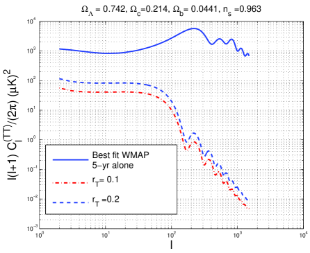
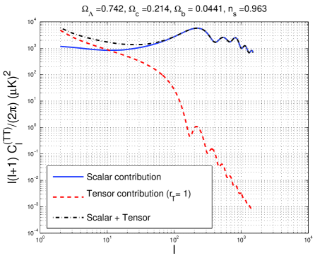
Figure 10: The temperature autocorrelations of the standard adiabatic scenario (full line) are compared with the TT angular power spectra induced by the tensor modes.

In both plots of Fig. 10 the full line denotes the TT angular power spectra corresponding to the best fit of the WMAP 5-yr data alone. In the plot at the left the dashed and dot-dashed lines illustrate, respectively, the cases $r_{\mathrm{T}}=0.1$ and $r_{\mathrm{T}}=0.2$. The tensor spectral index is fixed according to Eqs. (1.2) and (1.6) (see also Eqs. (6.4) and (6.5)). In both plots of Fig. 10 the spectral index does not run, i.e. $\alpha_{\mathrm{T}}=0$ in Eq. (1.6). Always in Fig. 10 (plot at the right) the dashed line denotes the tensor contribution in the case $r_{\mathrm{T}}=1$ while the dot-dashed line denotes the total TT angular power spectrum. The temperature and polarization observables can be obtained numerically (see, e.g. [91, 93]) but useful analytic results do exist in the literature [133, 134, 135, 136, 137]. An essential step for both approaches is to derive the angular power spectra in more explicit terms and as a function of the solution of the heat transfer equations. The solution of Eqs. (7.95), (7.96) and (7.97) can be formally written by using the integration along the line of sight which is also common to the scalar case (see, e.g. [119], for an introduction):

$$\Delta_{\mathrm{P}}(k,\mu,\tau_{0})=\int_{0}^{\tau_{0}}d\tau S_{\mathrm{P}}(k,\tau)e^{-i\mu x},$$ (7.126)

$$\Delta_{\mathrm{T}}(k,\mu,\tau_{0})=\int_{0}^{\tau_{0}}d\tau S_{\mathrm{T}}(k,\tau)e^{-i\mu x},$$ (7.127)

where $x=k(\tau_{0}-\tau)$. Note that $S_{\mathrm{T}}(k,\tau)$ and $S_{\mathrm{P}}(k,\tau)$ are related to the source terms of, respectively, Eqs. (7.95) and (7.96), i.e.

$$S_{\mathrm{P}}(k,\tau)=-{\mathcal{K}}(\tau)\,S(k,\tau),\qquad S_{\mathrm{T}}(k,\tau)=-h^{\prime}e^{-\epsilon(\tau,\tau_{0})}+{\mathcal{K}}(\tau)\,S(k,\tau),$$ (7.128)

where $S(k,\tau)$ is given by Eq. (7.97) and where

$${\mathcal{K}}(\tau)=\epsilon^{\prime}e^{-\epsilon(\tau,\tau_{0})},\qquad\epsilon(\tau,\tau_{0})=\int_{\tau}^{\tau_{0}}a\tilde{n}_{\mathrm{e}}\,x_{\mathrm{e}}\sigma_{\mathrm{T}}\,d\tau,\qquad\epsilon^{\prime}=a\tilde{n}_{\mathrm{e}}\,x_{\mathrm{e}}\sigma_{\mathrm{T}}.$$ (7.129)

is the visibility function expressed in terms of the differential optical depth $\epsilon^{\prime}$ and in terms of the optical depth $\epsilon(\tau,\tau_{0})$. The visibility function ${\mathcal{K}}(\tau)$ gives that probability that a photon is last scattered between $\tau$ and $\tau+d\tau$. In loose terms the visibility function is peaked around the redshift of recombination. In analytic discussions the visibility function is often approximated by means of a Gaussian profile (see, e. g., [120, 137, 119] and also [138, 139, 140, 141]):

$${\mathcal{K}}(\tau)={\mathcal{N}}(\sigma_{\mathrm{rec}})e^{-\frac{(\tau-\tau_{\mathrm{rec}})^{2}}{2\sigma_{\mathrm{rec}}^{2}}},\qquad\int_{0}^{\tau_{0}}{\mathcal{K}}(\tau)d\tau=1.$$ (7.130)

As indicated in Eq. (7.130), ${\mathcal{N}}(\sigma_{\mathrm{rec}})$ is determined by requiring that the integral of ${\mathcal{K}}(\tau)$ over $\tau$ is normalized to $1$. The WMAP data suggest a thickness (in redshift space) $\Delta z_{\mathrm{rec}}\simeq 195\pm 2$ [8] which would imply that $\sigma_{\mathrm{rec}}$, in units of the (comoving) angular diameter distance to recombination, can be estimated as $\sigma_{\mathrm{rec}}/\tau_{0}\simeq 1.43\times 10^{-3}$. When $\tau_{0}\gg\tau_{\mathrm{rec}}$ and $\tau_{0}\gg\sigma_{\mathrm{rec}}$ the normalization appearing in Eq. (7.130) can be estimated as ${\mathcal{N}}(\sigma_{\mathrm{rec}})\to\sigma_{\mathrm{rec}}^{-1}\,\sqrt{2/\pi}$. In [137] it has been suggested that a better approximation, for the case of the tensor modes, is to assume that ${\mathcal{K}}(\tau)$ has two different widths, respectively, for $\tau<\tau_{\mathrm{rec}}$ and for $\tau>\tau_{\mathrm{rec}}$. Recalling now Eq. (2.44) and (2.49) the $a_{\ell\,m}^{(\mathrm{T})}$ can be written as

$$a_{\ell\,m}^{(\mathrm{T})}=\int d\hat{n}\,Y_{\ell m}^{*}\,\Delta_{\mathrm{I}}(\hat{n})$$

$$=\frac{1}{(2\pi)^{3/2}}\int d^{3}k\,\int_{0}^{2\pi}d\varphi\int_{-1}^{1}\,d\mu(1-\mu^{2})[e^{2i\varphi}e_{1}(\vec{k})+e^{-2i\varphi}e_{2}(\vec{k})]Y_{\ell\,m}^{*}(\mu,\varphi)\Delta_{\mathrm{T}}(k,\mu,\tau_{0}),$$ (7.131)

where the second equality follows from the Fourier transform of $\Delta_{\mathrm{I}}(\hat{n})$ and by using Eq. (7.98) in the obtained expression. The angular integrations can now be performed with the approach already exploited in previous subsection for the polarization observables. It is however useful to solve Eq. (7.131) with a slightly different method (see, e. g. [91]) where explicit use is made of the solutions (7.126) and (7.127).

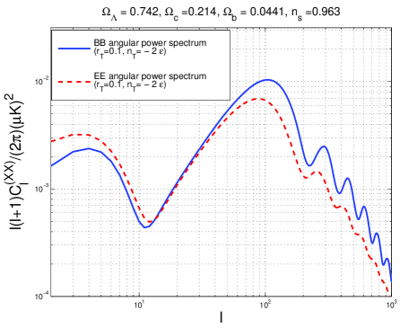
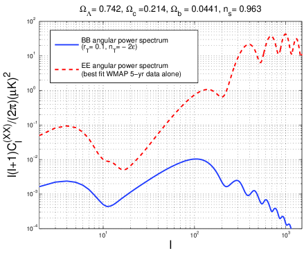
Figure 11: The polarization autocorrelations induced by the tensor modes are compared among themselves and with the EE angular power spectra produced by the adiabatic mode.

Indeed, inserting Eq. (7.126) into Eq. (7.131) $a^{(\mathrm{T})}_{\ell\,m}$ can be written as

$$a_{\ell\,m}^{(\mathrm{T})} = \frac{1}{(2\pi)^{3/2}}\int d^{3}k\,\int_{0}^{\tau_{0}}d\tau\,S_{\mathrm{T}}(k,\tau)[{\mathcal{I}}^{(\mathrm{T})}_{+}(\ell,m,x)e_{1}(\vec{k})+{\mathcal{I}}^{(\mathrm{T})}_{-}(\ell,m,x)e_{2}(\vec{k})],$$ (7.132)

$${\mathcal{I}}^{(\mathrm{T})}_{\pm}(\ell,m,x) = \int_{0}^{2\pi}d\varphi Y_{\ell\,m}^{*}(\mu,\varphi)(1-\mu^{2})e^{\pm 2i\varphi}e^{-i\mu x}.$$ (7.133)

In ${\mathcal{I}}^{(\mathrm{T})}_{\pm}$ the integration over $\varphi$ is trivial since the (ordinary) spherical harmonics depend upon $\varphi$ as $e^{im\varphi}$ (see, e. g., Eqs. (2.54) and (2.55)). Thus, as expected on the basis of the results of the previous subsection, ${\mathcal{I}}^{(\mathrm{T})}_{\pm}\propto 2\pi\delta_{m,\,\pm 2}$. The latter results allows for a simplification so that, for instance,

$${\mathcal{I}}^{(\mathrm{T})}_{+}(\ell,m,x) = 2\pi\delta_{m,\,2}\,\sqrt{\frac{2\ell+1}{4\pi}}\,\sqrt{\frac{(\ell-2)!}{(\ell+2)!}}\int_{-1}^{1}d\mu(1-\mu^{2})^{2}\,\frac{d^{2}P_{\ell}}{d\mu^{2}}e^{-i\mu x}$$ (7.134)

$$= -4\pi(-i)^{\ell}\delta_{m,\,2}\,\sqrt{\frac{2\ell+1}{4\pi}}\,\sqrt{\frac{(\ell-2)!}{(\ell+2)!}}(1+\partial_{x}^{2})^{2}[x^{2}j_{\ell}(x)],$$

where the second equality follows by first integrating by parts and by then expanding $e^{-i\mu x}$ in series of Legendre polynomials. Indeed, in Eq. (7.134), $j_{\ell}(x)$ are the spherical Bessel functions. Note, finally that, inside the integral of Eq. (7.134) expressions like $(1-\mu^{2})^{2}e^{-i\mu x}$ can be traded for $(1+\partial_{x}^{2})^{2}\,e^{-i\mu x}$. Recalling the properties of the associated Legendre (see second relation of Eq. (2.55)) the other integral, i.e. ${\mathcal{I}}^{(\mathrm{T})}_{-}(\ell,m,x)$ can be performed exactly in the same way. By making explicit the ensemble averages and by using Eq. (2.49), the angular power spectrum illustrated in Fig. 10 can be obtained and it is given by:

$$C_{\ell}^{(\mathrm{TT})} = 4\pi\int\frac{dk}{k}{\mathcal{P}}_{\mathrm{T}}(k)|\Delta_{\mathrm{T}\ell}(k,\tau_{0})|^{2},$$

$$\Delta_{\mathrm{T}\ell}(k,\tau_{0}) = \overline{N}_{\ell}\int_{0}^{\tau_{0}}S_{\mathrm{T}}(k,\tau)\frac{j_{\ell}(x)}{x^{2}},$$ (7.135)

where, as in Eq. (2.46), $\overline{N}_{\ell}=\sqrt{(\ell-2)!/(\ell+2)!}$. Having discussed the temperature autocorrelation induced by the long wavelength gravitons it is now the moment of discussing the polarization observables. In Fig. 11 (plot at the left) the EE angular power spectra (full line) are compared with the B-mode autocorrelations (dashed line) induced by the tensor modes in the case $r_{\mathrm{T}}=0.1$ while the other cosmological parameters are fixed to the best-fit values of the WMAp 5-yr data alone. Always in Fig. 11 (plot at the right) the full line illustrates the B-mode autocorrelation in the case $r_{\mathrm{T}}=0.1$ while the dashed line illustrated the EE angular power spectrum stemming from the standard adiabatic mode. In Fig. 12 (plot at the left) the BB angular power spectra are illustrated for different values of $r_{\mathrm{T}}$ compatible with current bounds on $r_{\mathrm{T}}$ (see Tabs. 1 and 2).

The E-mode and the B-mode angular power spectra can be obtained from Eqs. (7.99) and (7.100) by carefully following all the steps leading to the temperature autocorrelation of Eq. (7.135). The crucial difference will be, of course, that $a_{\ell\,m}^{(\mathrm{E})}$ and $a_{\ell\,m}^{(\mathrm{B})}$ arise, respectively, in the expansion of $\Delta_{\mathrm{E}}(\hat{n})$ and $\Delta_{\mathrm{B}}(\hat{n})$ as reported in Eq. (2.46). To compute $a_{\ell\,m}^{(\mathrm{E})}$ and $a_{\ell\,m}^{(\mathrm{B})}$ in terms of $S_{\mathrm{P}}(k,\tau)$ the steps are, in short, the following:

• $a_{\ell\,m}^{(\mathrm{E})}$ and $a_{\ell\,m}^{(\mathrm{B})}$ should be first expressed in terms of $\Delta_{\mathrm{E}}(\hat{n})$ and $\Delta_{\mathrm{B}}(\hat{n})$ as in Eq. (2.46);

• then Eqs. (7.99) and (7.100) should be inserted into Eqs. (2.65) and (2.66);

• the evolution for $\Delta_{\mathrm{P}}(k,\mu,\tau)$ can then be solved in Fourier space as in Eq. (7.126).

The first and the second step has been already (partially) performed in the previous subsection and the results have been given in Eqs. (7.103)–(7.104) with the difference that, now, the two polarizations can be treated simultaneously so that, in Fourier space,

$$\Delta_{\mathrm{Q}}(\vec{k},\tau,\mu,\varphi) = (1+\mu^{2})[e^{2i\varphi}e_{1}(\vec{k})+e^{-2i\varphi}e_{2}(\vec{k})]\Delta_{\mathrm{P}}(k,\tau,\mu),$$ (7.136)

$$\Delta_{\mathrm{U}}(\vec{k},\tau,\mu,\varphi) = 2\mu i[e^{2i\varphi}e_{1}(\vec{k})-e^{-2i\varphi}e_{2}(\vec{k})]\Delta_{\mathrm{P}}(k,\tau,\mu).$$ (7.137)

Note that Eqs. (7.136) and (7.137) follow directly from Eqs. (7.99) and (7.100) by definition of $\Delta_{\pm}(\vec{k},\tau,\mu,\varphi)$. It should be appreciated that one derivation with respect to $\varphi$ changes the azimuthal structure of $\Delta_{\mathrm{Q}}(\vec{k},\tau,\mu,\varphi)$ and $\Delta_{\mathrm{U}}(\vec{k},\tau,\mu,\varphi)$, i.e.

$$\partial_{\varphi}\Delta_{\mathrm{U}}=-4\mu[e^{2i\varphi}e_{1}(\vec{k})+e^{-2i\varphi}e_{2}(\vec{k})]\Delta_{\mathrm{P}}(k,\tau,\mu),$$ (7.138)

$$\partial_{\varphi}\Delta_{\mathrm{Q}}=2i(1+\mu^{2})[e^{2i\varphi}e_{1}(\vec{k})-e^{-2i\varphi}e_{2}(\vec{k})]\Delta_{\mathrm{P}}(k,\tau,\mu).$$ (7.139)

Using now Eqs. (7.136)–(7.137) and (7.138)–(7.139) inside Eqs. (7.103) and (7.104) we do get, after Fourier transform,

$$a^{(\mathrm{B})}_{\ell m} = -2i\frac{\overline{N}_{\ell}}{(2\pi)^{3/2}}\int d^{3}k\,\int_{0}^{2\pi}d\varphi\int_{-1}^{1}\,d\mu[e^{2i\varphi}e_{1}(\vec{k})-e^{-2i\varphi}e_{2}(\vec{k})]Y_{\ell\,m}^{*}(\mu,\varphi)$$ (7.140)

$$\times (1-\mu^{2})[\mu\partial_{\mu}^{2}+4\partial_{\mu}]\Delta_{\mathrm{P}}(k,\mu,\tau_{0}),$$

$$a^{(\mathrm{E})}_{\ell m} = -\frac{\overline{N}_{\ell}}{(2\pi)^{3/2}}\int d^{3}k\,\int_{0}^{2\pi}d\varphi\int_{-1}^{1}\,d\mu[e^{2i\varphi}e_{1}(\vec{k})+e^{-2i\varphi}e_{2}(\vec{k})]Y_{\ell\,m}^{*}(\mu,\varphi)$$ (7.141)

$$\times (1-\mu^{2})[(1+\mu^{2})\partial_{\mu}^{2}+8\mu\partial_{\mu}+12]\Delta_{\mathrm{P}}(k,\mu,\tau_{0}).$$

According to Eq. (7.126) $\Delta_{\mathrm{P}}(k,\mu,\tau_{0})$ can be related to $S_{\mathrm{P}}(k,\tau)$ and the resulting coefficients are:

$$a_{\ell\,m}^{(\mathrm{B})} = -\frac{\overline{N}_{\ell}}{(2\pi)^{3/2}}\int_{0}^{2\pi}d\varphi\int_{-1}^{1}d\mu Y_{\ell\,m}^{*}(\mu,\varphi)\int d^{3}k[e^{2i\varphi}e_{1}(\vec{k})-e^{-2i\varphi}e_{2}(\vec{k})]$$ (7.142)

$$\times (1-\mu^{2}){\mathcal{O}}_{\mathrm{B}}(x)\int_{0}^{\tau_{0}}S_{\mathrm{P}}(k,\tau)\,e^{-i\mu x}d\tau$$

$$a_{\ell\,m}^{(\mathrm{E})} = -\frac{\overline{N}_{\ell}}{(2\pi)^{3/2}}\int d\hat{n}Y_{\ell\,m}^{*}(\mu,\varphi)\int d^{3}k[e^{2i\varphi}e_{1}(\vec{k})+e^{-2i\varphi}e_{2}(\vec{k})]$$ (7.143)

$$\times (1-\mu^{2}){\mathcal{O}}_{\mathrm{E}}(x)\int_{0}^{\tau_{0}}S_{\mathrm{P}}(k,\tau)\,e^{-i\mu x}d\tau,$$

where ${\mathcal{O}}_{\mathrm{B}}(x)$ and ${\mathcal{O}}_{\mathrm{E}}(x)$ are two differential operators, i.e.

$${\mathcal{O}}_{\mathrm{B}}(x)=2x^{2}\partial_{x}^{2}+8x,\qquad{\mathcal{O}}_{\mathrm{E}}(x)=x^{2}(1-\partial_{x}^{2})-8x\partial_{x}-12.$$ (7.144)

Now Eqs. (7.142) and (7.143) can be used into Eqs. (2.48) and the angular power spectra become:

$$C_{\ell}^{(\mathrm{BB})}=4\pi\int\frac{dk}{k}{\mathcal{P}}_{\mathrm{T}}(k)|\Delta_{\mathrm{B}\ell}(k,\tau_{0})|^{2},$$ (7.145)

$$C_{\ell}^{(\mathrm{EE})}=4\pi\int\frac{dk}{k}{\mathcal{P}}_{\mathrm{T}}(k)|\Delta_{\mathrm{E}\ell}(k,\tau_{0})|^{2},$$ (7.146)

where

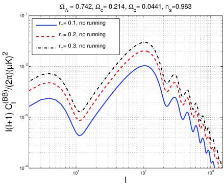
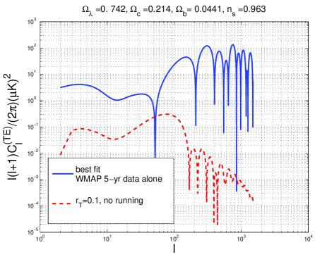
Figure 12: The B-mode autocorrelation for different values of $r_{\mathrm{T}}$ (plot at the left). The TE cross correlation induced by the tensor modes is compared with the corresponding angular power spectrum induced by the standard adiabatic mode.

$$\Delta_{\mathrm{E}\ell}(k,\tau_{0})=\biggl{[}\frac{4}{x}\partial_{x}j_{\ell}(x)+\frac{2}{x^{2}}j_{\ell}(x)+\partial^{2}_{x}j_{\ell}(x)-j_{\ell}(x)\biggr{]}\int_{0}^{\tau_{0}}d\tau S_{\mathrm{P}}(k,\tau),$$ (7.147)

$$\Delta_{\mathrm{B}\ell}(k,\tau_{0})=\biggl{[}2\partial_{x}j_{\ell}(x)+\frac{4}{x^{2}}j_{\ell}(x)\biggr{]}\int_{0}^{\tau_{0}}d\tau S_{\mathrm{P}}(k,\tau).$$ (7.148)

The tensor modes also induce a TE angular power spectrum (i.e. a cross-correlation between the temperature and the E-mode polarization). In Fig. 12 (plot at the right) the absolute value of the TE (tensor) angular power spectrum is compared with the corresponding angular power spectrum induced by the standard adiabatic mode. The cross-correlation between temperature and polarization can be obtained inserting Eqs. (7.133) and (7.141) into Eq. (2.49) and the result is

$$C_{\ell}^{(\mathrm{TE})}=4\pi\int\frac{dk}{k}{\mathcal{P}}_{\mathrm{T}}(k)\Delta_{\mathrm{E}\ell}(k,\tau_{0})\Delta_{\mathrm{T}\ell}(k,\tau_{0}),$$ (7.149)

where, $\Delta_{\mathrm{T}\ell}(k,\tau_{0})$ and $\Delta_{\mathrm{E}\ell}(k,\tau_{0})$ are given, respectively, by Eqs. (7.135) and (7.147). It should finally be mentioned that the derivatives with respect to $x$ appearing in Eqs. (7.147) and (7.148) can be transformed into derivatives with respect to $\tau$ by making use of integration by parts [91]. This step is carried on in full analogy with what happens with the scalar modes of the geometry [119].

Various experiments provided, so far, direct limits on the B-mode polarization.

Experiments	Years	Pivot frequencies	Upper limits on BB
Dasi [21, 22, 23]	2000-2003	$26$–$36$ GHz	$\ell(\ell+1)C_{\ell}^{(\mathrm{BB})}(2\pi)\leq 50\,(\mu\,\mathrm{K})^{2}$
Boomerang [142]	2003	$145$ GHz	$\ell(\ell+1)C_{\ell}^{(\mathrm{BB})}/(2\pi)\leq 8.6\,(\mu\,\mathrm{K})^{2}$
Maxipol [143, 144]	2003	$140$ GHz	$\ell(\ell+1)C_{\ell}^{(\mathrm{BB})}/(2\pi)\leq 112.3\,(\mu\,\mathrm{K})^{2}$
Quad [28, 29, 30]	2007	$100$/ $150$ GHz	$\ell(\ell+1)C_{\ell}^{(\mathrm{BB})}/(2\pi)\leq 10\,(\mu\,\mathrm{K})^{2}$
Cbi [26, 27]	2002-2005	$26$–$36$ GHz	$\ell(\ell+1)C_{\ell}^{(\mathrm{BB})}/(2\pi)\leq 3.76\,(\mu\,\mathrm{K})^{2}$
Capmap [24, 25]	2004-2005	$35$–$46$/$84$–$100$ GHz	$\ell(\ell+1)C_{\ell}^{(\mathrm{BB})}/(2\pi)\leq 4.8\,(\mu\,\mathrm{K})^{2}$
Wmap [3, 4, 6]	2001-2006	$23$–$94$ GHz	$\ell(\ell+1)C_{\ell}^{(\mathrm{BB})}/(2\pi)\leq 0.15\,(\mu\,\mathrm{K})^{2}$

Table 3: The main polarization experiments, their typical observational frequencies, and the upper limits on the B-mode polarization are illustrated.

The limits on $r_{\mathrm{T}}$ reported in Tabs. 1 and 2 follow from a combined analysis of the TT, EE and TE angular power spectra which allows for a tensor contribution. As Tab. 3 indicates the upper limits on the B-mode polarization are still rather loose and, often, derived on the basis of a limited range of harmonics.

8 High-frequency spikes in the relic graviton background

In the $\Lambda$CDM paradigm long wavelength gravitons can affect the CMB polarization. As the frequency increases towards the region accessible to wide band interferometers, the $\Lambda$CDM signal can only decrease for number of independent reasons:

• in the $\Lambda$CDM paradigm the spectral energy density is only approximately scale-invariant (see, e.g. Fig. 2) but the scaling violations always tend to make the spectral energy density smaller at high frequencies;

• there are various secondary effects associated, for instance, with the variation of the effective number of relativistic degrees of freedom, with the neutrino anisotropic stress and with the transition to a phase dominated by the dark-energy contribution: all these features reduce the spectral energy density in different frequency regions;

• the addition of supplementary scalar fields driving the inflationary phase does not change the two previous statements.

The previous conclusions are all based (either directly or indirectly) on the assumption that the thermal history of the Universe is minimal in the sense that, after inflation, the Universe soon becomes dominated by relativistic particles so that the sound speed of the plasma soon reaches values $c_{\mathrm{st}}=1/\sqrt{3}$. The post-inflationary thermal history might not be minimal. For instance it could happen that the transition to the radiation-dominated regime is not instantaneous [75]. More specifically it can happen that, after inflation, the sound speed of the plasma is such that $c_{\mathrm{st}}>1/\sqrt{3}$. When the sound speed is larger than $1/\sqrt{3}$, the fluid is said to be stiff. In the system of units used in the present paper the speed of light is such that $c=1$. A natural upper limit for the sound speed is exactly $1$ which is the maximally stiff fluid compatible with causality [124] (see, however, also [125]). If the thermal history of the Universe contemplates a post-inflationary phase stiffer than radiation, a spike in the relic graviton spectrum is expected at high frequencies [75] (see also [76, 77] as well as Eqs. (6.29)–(6.30) and discussion therein). The possibility of having a post-inflationary phase stiffer than radiation has been also investigated in different contexts such as in [146, 147, 148].

In the early Universe, the dominant energy condition might be violated and this observation will also produce scaling violations in the spectral energy density [149]. If we assume the validity of the $\Lambda$CDM paradigm, a violation of the dominant energy condition implies that, during an early stage of the life of the Universe, the effective enthalpy density of the sources driving the geometry was negative and this may happen in the presence of bulk viscous stresses [149] (see also [150, 151] for interesting reprises of this idea). In what follows the focus will be on the more mundane possibility that the thermal history of the plasma includes a phase where the speed of sound was close to the speed of light.

Absent any indirect tests on the thermal history of the Universe prior to the formation of light nuclear elements, it is legitimate to investigate situations where, before nucleosyntheis, the sound speed of the plasma was larger than $1/\sqrt{3}$, at most equalling the speed of light. In this plausible extension of the current cosmological paradigm, hereby dubbed Tensor-$\Lambda$CDM (i.e. T$\Lambda$CDM) scenario, high-frequency gravitons are copiously produced [40, 41]. Without conflicting with the bounds on the tensor to scalar ratio stemming from the combined analysis of the three standard cosmological data sets (i.e. cosmic microwave background anisotropies, large-scale structure data and observations of type Ia supenovae), the spectral energy density of the relic gravitons in the T$\Lambda$CDM scenario can be potentially observable by wide-band interferometers (in their advanced version) operating in a frequency window which ranges between few Hz and few kHz.

The presence of a stiff phase increases the spectral energy density for frequencies larger than a pivotal frequency $\nu_{\mathrm{s}}$ which is related to the total duration of the stiff phase. If the stiff phase takes place before BBN, then $\nu_{\mathrm{s}}>10^{-2}$ nHz. If the stiff phase takes place for equivalent temperatures larger than $100$ GeV, then $\nu_{\mathrm{s}}\geq\mu\mathrm{Hz}$. If the stiff phase takes place for $T\geq 100$ TeV, then $\nu_{\mathrm{s}}>\mathrm{mHz}$. The frequency $\nu_{\mathrm{s}}$ marks the beginning of a branch of the spectrum where the tilt of the spectral energy density is blue (i.e. increasing in slope) rather than nearly scale invariant or slightly red (as it is the case in the conventional scenario).

8.1 Scaling violations

In the $\Lambda$CDM paradigm, for frequencies larger than $\nu_{\mathrm{eq}}$ the spectral energy density of the relic gravitons is, approximately, scale invariant (see Fig. 2). In the context of the T$\Lambda$CDM scenario the approximate scale-invariance of the flat plateau is violated. This situation is illustrated, for instance, in Fig. 4. In the present subsection a more detailed account of the typical frequencies of the problem will be presented. If there is some delay between the end of inflation and the onset of radiation the maximal wavenumber of the spectrum will be given by:

$$k_{\mathrm{max}}=M_{\mathrm{P}}\biggl{(}\frac{H}{M_{\mathrm{P}}}\biggr{)}^{1-\alpha}\biggr{(}\frac{H_{\mathrm{r}}}{M_{\mathrm{P}}}\biggl{)}^{\alpha-1/2}\biggl{(}\frac{H_{\mathrm{eq}}}{M_{\mathrm{P}}}\biggr{)}^{1/2}\biggl{(}\frac{a_{\mathrm{eq}}}{a_{0}}\biggr{)}$$ (8.1)

where $\alpha=2/[3(w_{\mathrm{t}}+1)]$ (with $w_{\mathrm{t}}>1/3$) is related to the specific kind of stiff dynamics. Equation (8.1) can also be written as

$$k_{\mathrm{max}}=M_{\mathrm{P}}\Sigma^{-1}\biggl{(}\frac{H_{\mathrm{eq}}}{M_{\mathrm{P}}}\biggr{)}^{1/2}\biggl{(}\frac{a_{\mathrm{eq}}}{a_{0}}\biggr{)}.$$ (8.2)

where

$$\Sigma=\biggl{(}\frac{H}{M_{\mathrm{P}}}\biggr{)}^{\alpha-1}\biggr{(}\frac{H_{\mathrm{r}}}{M_{\mathrm{P}}}\biggl{)}^{1/2-\alpha}.$$ (8.3)

In the case $\Sigma={\mathcal{O}}(1)$ (as it happens in the case $\alpha=1/3$ if the initial radiation is in the form of quantum fluctuations) $\nu_{\mathrm{max}}=k_{\mathrm{max}}/(2\pi)\simeq 100\,\,\mathrm{GHz}$, more precisely:

$$\nu_{\mathrm{max}}=1.177\times 10^{11}\Sigma^{-1}\biggl{(}\frac{h_{0}^{2}\Omega_{\mathrm{R}0}}{4.15\times 10^{-5}}\biggr{)}^{1/4}\,\,\mathrm{Hz}.$$ (8.4)

On top of the standard parameters of the $\Lambda$CDM scenario (see, e. g., Eq. (2.7)) the minimal T$\Lambda$CDM scenario demands two supplementary parameters

• the frequency $\nu_{\mathrm{s}}$ defining the region of the spectrum at which the scaling violations take place;

• the slope of the spectrum arising during the stiff phase.

The frequency $\nu_{\mathrm{s}}$ can be dynamically related to the frequency of the maximum and, consequently, the first parameter can be trated for $\Sigma$. As it will be shown in a moment, typical values for $\Sigma$ range between $0.01$ and $0.5$. The slope of the spectrum during the stiff phase depends upon the total barotropic index and can therefore be traded for $w_{\mathrm{t}}$. The curvature scale $H_{\mathrm{r}}$ determines $k_{\mathrm{s}}$ (or $\nu_{\mathrm{s}}$), i.e. the frequency at which the spectral energy density starts increasing. Supposing that from the end of inflation there is a single stiff phase (as it is natural to assume in a minimalistic persepective) the value of $k_{\mathrm{s}}$ is

$$k_{\mathrm{s}}=M_{\mathrm{P}}\biggl{(}\frac{H_{\mathrm{eq}}}{M_{\mathrm{P}}}\biggr{)}^{1/2}\biggl{(}\frac{a_{\mathrm{eq}}}{a_{0}}\biggr{)}\sqrt{\frac{H_{\mathrm{r}}}{M_{\mathrm{P}}}}.$$ (8.5)

Using the relation of $H_{\mathrm{r}}$ to $\Sigma$, Eq. (8.5) can also be written as

$$k_{\mathrm{s}}=M_{\mathrm{P}}\biggl{(}\frac{H_{\mathrm{eq}}}{M_{\mathrm{P}}}\biggr{)}^{1/2}\biggl{(}\frac{a_{\mathrm{eq}}}{a_{0}}\biggr{)}\Sigma^{1/(1-2\alpha)}\biggl{(}\frac{H}{M_{\mathrm{P}}}\biggr{)}^{(\alpha-1)/(2\alpha-1)}.$$ (8.6)

and as

$$\nu_{\mathrm{s}}=1.173\times 10^{11}\Sigma^{1/(1-2\alpha)}\,\,(\pi\epsilon{\mathcal{A}}_{{\mathcal{R}}})^{\frac{\alpha-1}{2(2\alpha-1)}}\,\,\biggl{(}\frac{h_{0}^{2}\Omega_{\mathrm{R}0}}{4.15\times 10^{-5}}\biggr{)}^{1/4}\,\,\mathrm{Hz}.$$ (8.7)

The quantity $\Sigma$ which parametrizes the location, in the spectrum, where the scaling violations appear must be smaller than $1$ or, at most, of order $1$. This is what happens within specific models. For instance, if the radiation present at the end of inflation comes from amplified quantum fluctuations (i.e. Gibbons-Hawking radiation), quite generically, at the end of inflation $\rho_{\mathrm{r}}\simeq H^{4}$. More specifically

$$\rho_{\mathrm{r}}=\frac{\pi^{2}}{30}N_{\mathrm{eff}}T_{H}^{4}=\frac{N_{\mathrm{eff}}H^{4}}{480\pi^{2}}.$$ (8.8)

In Eq. (8.8) $N_{\mathrm{eff}}$ is the number of species contributing to the quantum fluctuations during the quasi-de Sitter stage of expansion. In [128] (see also [76, 77, 78]) it has been argued that this quantity could be evaluated using a perturbative expansion valid in the limit of quasi-conformal coupling. It should be clear that $N_{\mathrm{eff}}$ is conceptually different from the number of relativistic degrees of freedom $g_{\rho}$. Given $H$ and $N_{\mathrm{eff}}$ the length of the stiff phase is fixed, in this case, by [78]

$$\lambda H^{4}\biggl{(}\frac{a_{\mathrm{i}}}{a_{\mathrm{r}}}\biggr{)}^{4}=H^{2}M_{\mathrm{P}}^{2}\biggl{(}\frac{a_{\mathrm{i}}}{a_{\mathrm{r}}}\biggr{)}^{3(w+1)}=H^{2}M_{\mathrm{P}}^{2}\biggl{(}\frac{a_{\mathrm{i}}}{a_{\mathrm{r}}}\biggr{)}^{2/\alpha},$$ (8.9)

where we used the fact that $\alpha=2/[3(w+1)]$ and where we defined $\lambda=N_{\mathrm{eff}}/(480\pi^{2})$. Equation (8.9) implies that

$$\biggl{(}\frac{a_{\mathrm{i}}}{a_{\mathrm{r}}}\biggr{)}=\lambda^{\frac{\alpha}{2-4\alpha}}\biggl{(}\frac{H}{M_{\mathrm{P}}}\biggr{)}^{\frac{\alpha}{1-2\alpha}}.$$ (8.10)

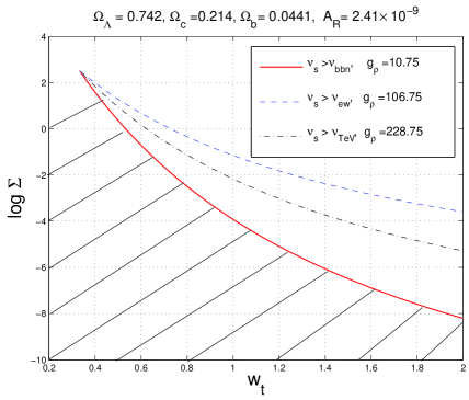
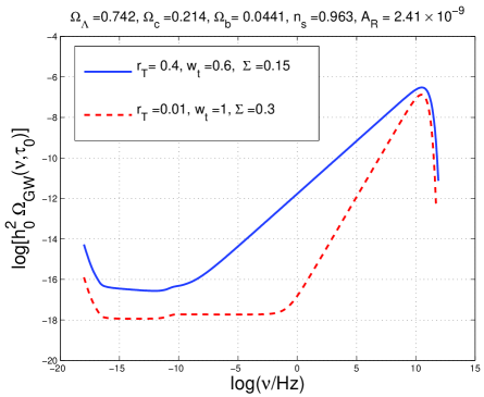
Figure 13: The bounds on $\nu_{\mathrm{s}}$ in the $(\Sigma,w_{\mathrm{t}})$ plane; the spectral energy density of the relic gravitons in the T$\Lambda$CDM scenario.

Recalling that $H_{\mathrm{r}}=H(a_{\mathrm{i}}/a_{\mathrm{r}})^{1/\alpha}$, we also have that Eq. (8.10) implies

$$\biggl{(}\frac{H_{\mathrm{r}}}{M_{\mathrm{P}}}\biggr{)}=\lambda^{\frac{1}{2(1-2\alpha)}}\biggl{(}\frac{H}{M_{\mathrm{P}}}\biggr{)}^{\frac{2(1-\alpha)}{(1-2\alpha)}}.$$ (8.11)

Using Eq. (8.11) and the definition of $\Sigma$ (see Eq. (8.3)) it turns out that $\Sigma=\lambda^{1/4}$, which is always smaller than $1$ and, at most, ${\mathcal{O}}(1)$.

Instead of endorsing an explicit model by pretending to know the whole thermal history of the Universe in reasonable detail, it is more productive to keep $\Sigma$ as a free parameter and to require that the scaling violations in the spectral energy density will take place before BBN. Consequently the variation of $\Sigma$, $w$ and $r_{\mathrm{T}}$ can be simultaneously bounded [40, 41]. If the stiff dynamics takes place before big-bang nucleosynthesis, then $\nu_{\mathrm{s}}>\nu_{\mathrm{bbn}}$ (see also Eq. (6.61)). This requirement guarantees that the stiff dynamics will be over by the time light nuclei start being formed. In a complementary approach one might also require that $\nu_{\mathrm{s}}>\nu_{\mathrm{ew}}$ where $\nu_{\mathrm{ew}}$ corresponds to the value of the Hubble rate at the electroweak epoch, i.e.

$$k_{\mathrm{ew}} = 2.5764\times 10^{9}\biggl{(}\frac{g_{\rho}}{106.75}\biggr{)}^{1/4}\biggl{(}\frac{T_{*}}{100\,\,\mathrm{GeV}}\biggr{)}\biggl{(}\frac{h_{0}^{2}\Omega_{\mathrm{R}0}}{4.15\times 10^{-5}}\biggr{)}^{1/4}\,\,\mathrm{Mpc}^{-1}$$ (8.12)

$$\nu_{\mathrm{ew}} = 3.998\times 10^{-6}\biggl{(}\frac{g_{\rho}}{106.75}\biggr{)}^{1/4}\biggl{(}\frac{T_{*}}{100\,\,\mathrm{GeV}}\biggr{)}\biggl{(}\frac{h_{0}^{2}\Omega_{\mathrm{R}0}}{4.15\times 10^{-5}}\biggr{)}^{1/4}\,\,\mathrm{Hz}.$$ (8.13)

Finally, yet a different requirement could be to impose that $\nu>\nu_{\mathrm{Tev}}$ where $\nu_{\mathrm{TeV}}$ is defined as

$$\nu_{\mathrm{TeV}}=4.819\times 10^{-3}\biggl{(}\frac{g_{\rho}}{228.75}\biggr{)}^{1/4}\biggl{(}\frac{T_{*}}{100\,\,\mathrm{TeV}}\biggr{)}\biggl{(}\frac{h_{0}^{2}\Omega_{\mathrm{R}0}}{4.15\times 10^{-5}}\biggr{)}^{1/4}\,\,\mathrm{Hz}.$$ (8.14)

The latter requirement would imply that the stiff age is already finished by the time the Universe has a temperature of the order of $100$ TeV when, presumably, the number of relativistic degrees of freedom was much larger than in the minimal standard model (in Eq. (8.14) the typical value of $g_{\rho}$ is the one arising in the minimal supersymmetric extension of the standard model).

In Fig. 13 (plot at the left) the constraints on $\Sigma$, $w_{\mathrm{t}}$ are illustrated. The value of $\Sigma$ controls the position of the frequency at which the nearly scale-invariant slope of the spectrum will be violated. The barotropic index $w_{\mathrm{t}}$ is taken to be always larger than $1/3$ and with a maximal value of $1$. The shaded region corresponds to the region excluded in the most constraining case, i.e. the one demanding $\nu_{\mathrm{s}}>\nu_{\mathrm{bbn}}$. Also the values of $r_{\mathrm{T}}$ are bounded by the same kind of considerations. Indeed, $\nu_{\mathrm{s}}$ depends upon $\epsilon$ which is related to $r_{\mathrm{T}}$ (see, e.g., Eq. (8.7)). Therefore, a lower bound on $\nu_{\mathrm{s}}$ also implies a bound in the ($r_{\mathrm{T}},\,w_{\mathrm{t}}$) plane.

8.2 Spectral energy density in the minimal T$\Lambda$CDM scenario

In Fig. 13 (plot at the right) two examples of the scaling violations on the spectral energy density are illustrated. Both examples are compatible with the bounds illustrated in the plot at the left. Similar examples have been already illustrated in Fig. 4. These examples will now be discussed in greater detail. The spectral energy density has been computed by using the numerical approach presented in section 6.

In the two examples of Fig. 13 (plot at the right) the $\Lambda$CDM parameters are fixed to the values reported in Eq. (2.7) (see [3, 4, 5, 6, 7]). The spectral index has been allowed to run, i.e. $\alpha_{\mathrm{T}}\neq 0$ (see Eqs. (1.6) and (6.53)). The two supplementary parameters should be identified with the sound speed during the stiff phase (i.e. $c_{\mathrm{st}}$) and the threshold frequency (i.e. $\nu_{\mathrm{s}}$). Besides $c_{\mathrm{st}}$ and $\nu_{\mathrm{s}}$, there will also be $r_{\mathrm{T}}$ which controls, at once, the normalization and the slope of the low-frequency branch of the spectral energy density. At the moment wide band interferometers have sensitivities which are insufficient for cutting through the phenomenologically interesting region [63, 64, 65]. In the near future, however, there is the hope of a dramatic improvement of the sensitivity: even 5 or 6 orders of magnitude at least heeding the original design (see e.g. [55]) together with the recent proposals for an advanced Ligo program.

As specifically discussed in Eqs. (8.5)–(8.6) the frequency of the elbow, i.e. $\nu_{\mathrm{s}}$, is fully determined by $\Sigma$ (see Eq. (8.3) and discussion therein). The two supplementary parameters $\nu_{\mathrm{s}}$ and $c_{\mathrm{st}}$ can be traded for $\Sigma$ and $w_{\mathrm{t}}$ as already done in Fig. 13 (plot at the left). In doing so there is also a potential advantage since, according to Eq. (8.4), $\Sigma$ shifts the maximal frequency of the spectrum.

As soon as the frequency increases from the aHz up to the nHz (and even larger) the spectral energy density increases sharply in comparison with the nearly scale-invariant case where the spectral energy density was, for $\nu>\mathrm{nHz}$, at most ${\mathcal{O}}(10^{-16})$. In the case of Fig. 13 the spectral energy density is clearly much larger. The accuracy in the determination of the infra-red branch of the spectrum is a condition for the correctness of the estimate of the spectral energy density of the high-frequency branch. The plots of Fig. 13 (see also Fig. 4) demonstrate that the low-frequency bounds on $r_{\mathrm{T}}$ do not forbid a larger signal at higher frequencies.

A decrease of $r_{\mathrm{T}}$ implies a suppression of the nearly scale-invariant plateau in the region $\nu_{\mathrm{eq}}<\nu<\nu_{\mathrm{s}}$. At the same time the amplitude of the spectral energy density still increases for frequencies larger than the frequency of the elbow (i.e. $\nu_{\mathrm{s}}$). The latter trend can be simply understood since, at high frequency, the transfer function for the spectral energy density grows faster than the power spectrum of inflationary origin. For instance, in the case $w_{\mathrm{t}}=1$ and neglecting logarithmic corrections, $\Omega_{\mathrm{GW}}(\nu,\tau_{0})\propto\nu^{n_{\mathrm{T}}+1}$ for $\nu\gg\nu_{\mathrm{s}}$. Now, recall that $n_{\mathrm{T}}$ is given by Eq. (1.4). If $r_{\mathrm{T}}\to 0$, the combination $(n_{\mathrm{T}}+1)$ will be much closer to $1$ than in the case when, say, $r_{\mathrm{T}}\simeq 0.3$. This aspect can be observed in Fig. 4 where different values of $r_{\mathrm{T}}$ have been reported. By decreasing the $w_{\mathrm{t}}$ from $1$ to, say, $0.6$ the extension of the nearly flat plateau gets narrower. This is also a general effect which is particularly evident by comparing the two curves of Fig. 13 (plot at the right).

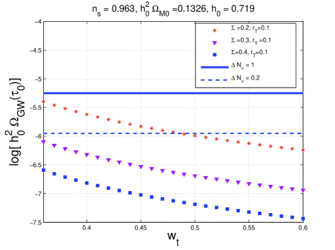
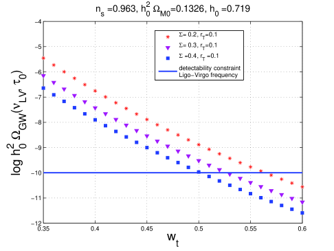
Figure 14: The bounds stemming from the amount of extra-relativistic species at the epoch of the synthesis of light nuclei are applied to the relic graviton spectra from the stiff epoch (plot at the left). The detectability constraint (full line in the plot at the right) stemming from the putative sensitivities of wide-band interferometers in their advanced version. The points corresponding to the spectral energy density should lie above the full lines to be potentially interesting for those instruments.

The slope of the high-frequency branch of the graviton energy spectrum can be easily deduced with analytic methods and it turns out to to be

$$\frac{d\ln{\Omega_{\mathrm{GW}}}}{d\ln{\nu}}=\frac{6w_{\mathrm{t}}-2}{3w_{\mathrm{t}}+1},\qquad\nu>\nu_{\mathrm{s}},$$ (8.15)

up to logarithmic corrections. The result of Eq. (8.15) stems from the simultaneous integration of the background evolution equations and of the tensor mode functions according to the techniques described in section 3. The semi-analytic estimate of the slope (see [75]) agrees with the results obtained by means of the transfer function of the spectral energy density.

To conclude the discussion it is appropriate to elaborate on the interplay between the stiff spectra and the phenomenological bounds mentioned in subsection 1.6. Let us start with millisecond pulsar bound of Eq. (1.14).

Assuming the maximal growth of the spectral energy density and the minimal value of $\nu_{\mathrm{s}}$, i.e. $\nu_{\mathrm{bbn}}$ we will have

$$h_{0}^{2}\Omega_{\mathrm{GW}}(\nu,\tau_{0})\propto\nu,\qquad\nu\geq\nu_{\mathrm{s}}\simeq\nu_{\mathrm{bbn}}.$$ (8.16)

Since $\nu_{\mathrm{pulsar}}\simeq 10^{3}\nu_{\mathrm{bbn}}$, Eq. (8.16) implies that $h_{0}^{2}\Omega_{\mathrm{GW}}(\nu_{\mathrm{pulsar}},\tau_{0})\simeq 10^{-13}$ or even $10^{-14}$ depending upon $r_{\mathrm{T}}$. But this value is always much smaller than the constraint stemming from pulsar timing measurements (see Eq. (1.14)). If either $\nu_{\mathrm{s}}\gg\nu_{\mathrm{bbn}}$ or $c_{\mathrm{st}}<1$ the value of $h_{0}^{2}\Omega_{\mathrm{GW}}(\nu_{\mathrm{pulsar}},\tau_{0})$ will be even smaller. Consequently, even in the extreme cases when the frequency of the elbow is close to $\nu_{\mathrm{bbn}}$, the spectral energy density is always much smaller than the requirement of Eq. (1.14).

As noticed in the past [121, 75], the most significant constraint on the stiff spectra stems from BBN. The models illustrated in Fig. 13 (plot at the right) are on the verge of saturating the bounds of Eqs. (1.18)–(1.19). This conclusion stems directly from the form of spectral energy density: the broad spike dominates the (total) energy density of relic gravitons which are inside the Hubble radius at the time of big bang nucleosynthesis. For consistency with the low-frequency determinations of the tensor power spectrum $r_{\mathrm{T}}$ must be bounded from above according to the values reported, for instance, in Tabs. 1 and 2. Once the the value of $r_{\mathrm{T}}$ has been selected, the constraints of Eqs. (1.18)–(1.19) can be imposed. From Fig. 13 a large signal is expected for $\nu_{\mathrm{LV}}\simeq 100$ Hz for $0.35<w_{\mathrm{t}}<0.6$. This range turns out to be compatible with the bounds of Eqs. (1.18)–(1.19). In the opposite limit (e. g. $w_{\mathrm{t}}\simeq 1$) the spike becomes narrower, the elbow frequency augments and the signal at the interferometer scale diminishes.

In Fig. 14 the energy density of the relic gravitons inside the Hubble radius at the nucleosynthesis epoch is reported in the case $r_{\mathrm{T}}=0.1$ and for different values of $\Sigma$. In the plot at the left $n_{\mathrm{s}}=0.963$ as implied by the WMAP 5-yr data alone. The acceptable region of the parameter space must stay below the horizontal lines which illustrate different values of $\Delta N_{\nu}$ (see Eqs. (1.18)–(1.19)). As the scalar spectral index diminishes, the constraints are better satisfied since $n_{\mathrm{s}}$ controls $\alpha_{\mathrm{T}}$ and, consequently, the frequency dependence of the tensor spectral index $n_{\mathrm{T}}$ (see Eq. (1.4)) in the case $\alpha_{\mathrm{T}}\neq 0$.

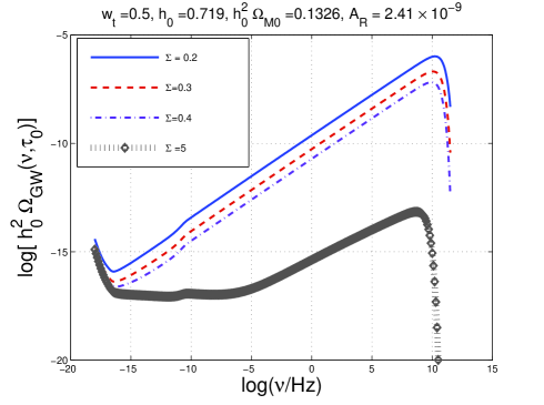
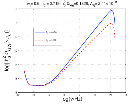
Figure 15: The spectral energy density is illustrated for small values of $w_{\mathrm{t}}$ and different values of $\Sigma$ (plot at the left). In the plot at the right $\Sigma=0.2$ and $w_{\mathrm{t}}=0.6$.

8.3 Detectability prospects

By lowering $w_{\mathrm{t}}$, $h_{0}^{2}\Omega_{\mathrm{GW}}(\nu,\tau_{0})$ increases for $\nu=\nu_{\mathrm{LV}}\simeq 0.1\,\mathrm{kHz}$. This trend can be inferred from Fig. 14 (plot at the right) where the spectral energy density is evaluated exactly for $\nu=\nu_{\mathrm{LV}}$. To be detectable by wide band interferometers the parameters of the T$\Lambda$CDM must lie above the full lines. The region of low barotropic indices emerging neatly from Fig. 14, leads to spectral energy densities which are progressively flattening as $w_{\mathrm{t}}$ diminishes towards $1/3$. Low values of $w_{\mathrm{t}}$ bring the frequency of the elbow, i.e. $\nu_{\mathrm{s}}$ below $10^{-10}$ Hz which is unacceptable since it would mean that, during nucleosynthesis, the Universe was dominated by the stiff fluid. In Fig. 13 (plot at the left) the region above the full line corresponds to a range of parameters for which $\nu_{\mathrm{s}}>\nu_{\mathrm{bbn}}$: in such a range a decrease of $w_{\mathrm{t}}$ demands an increase of $\Sigma$. The latter occurrence is illustrated in Fig. 15 where, at the left, $w_{\mathrm{t}}=0.5$. The full, dashed and dot-dashed curves illustrated in Fig. 15 (plot at the left) are incompatible with the phenomenological constraints since the frequency of the elbow is systematically smaller than $\nu_{\mathrm{bbn}}$. Once more, this choice of parameters would contradict the bounds of Fig. 13 and would imply that the stiff phase is not yet finished at the BBN time. In the left plot of Fig. 15 the diamonds denote a model which is compatible with BBN considerations but whose signal at the frequency of interferometers is rather small (always three orders of magnitude larger than in the case of conventional inflationary models).

The compatibility with the phenomenological constraints demands that the parameters of the T$\Lambda$CDM paradigm must lie above the full lines of Fig. 13 (plot at the left). The requirements of Fig. 13 suggest, therefore, that $\Sigma$ should be raised a bit. In this case the frequency of the elbow gets shifted to the right but, at the same time, the overall amplitude of the spike diminishes. The putative amplitude remains still much larger than the conventional inflationary signal reported, for instance, in Fig. 3.

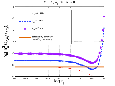
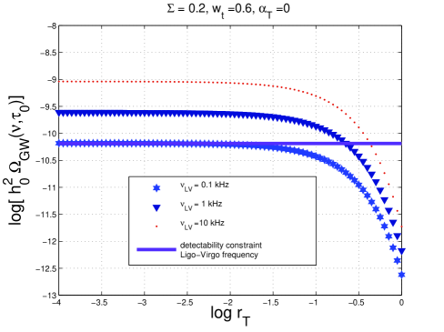
Figure 16: The graviton energy spectrum is illustrated, in the T$\Lambda$CDM scenario, for $\nu=\nu_{\mathrm{LV}}$ and as a function of $r_{\mathrm{T}}$ (plot at the left) in the case $\alpha_{\mathrm{T}}\neq 0$. In the plot at the right $\alpha_{\mathrm{T}}=0$.

In Fig. 16 the spectral energy density of the relic gravitons is illustrated as a function of $r_{\mathrm{T}}$ for a choice of parameters which is compatible with all the bounds applicable to the stochastic backgrounds of the relic gravitons. The three curves refer to three different frequencies, i.e. $0.1$ kHz, $1$ kHz and $10$ kHz. Indeed, if the spectrum is nearly scale-invariant (as in the case o Fig. 3) we can compare the potential signal with the central frequency of the window. If the signal increases with frequency it is interesting to plot the same curve for some significant frequencies inside the window of wide-band interferometers. Even if the frequency window extends from few Hz to $10$ kHz the maximal sensitivity is in the central region and depends upon various important factors which will now be briefly discussed.

To illustrate more quantitatively this point we remind the expression of the signal-to-noise ratio (SNR) in the context of optimal processing required for the detection of stochastic backgrounds:

$${\rm SNR}^{2}\,=\,\frac{3H_{0}^{2}}{2\sqrt{2}\,\pi^{2}}\,F\,\sqrt{T}\,\left\{\,\int_{0}^{\infty}\,{\rm d}\nu\,\frac{\gamma^{2}(\nu)\,\Omega^{2}_{{\rm GW}}(\nu,\tau_{0})}{\nu^{6}\,S_{n}^{\,(1)}(\nu)\,S_{n}^{\,(2)}(\nu)}\,\right\}^{1/2}\;,$$ (8.17)

($F$ depends upon the geometry of the two detectors and in the case of the correlation between two interferometers $F=2/5$; $T$ is the observation time). In Eq. (8.17), $S_{n}^{\,(k)}(f)$ is the (one-sided) noise power spectrum (NPS) of the $k$-th $(k=1,2)$ detector. The NPS contains the important informations concerning the noise sources (in broad terms seismic, thermal and shot noises) while $\gamma(\nu)$ is the overlap reduction function which is determined by the relative locations and orientations of the two detectors. In [68] Eq. (8.17) has been used to assess the detectability prospects of gravitons coming from a specific model of stiff evolution with $w_{\mathrm{t}}=1$. At that time the various suppressions of the low-frequency amplitude as well as the free-streaming effects were not taken into account. Furthermore, the evaluation of the energy transfer function was obtained, in [70], not numerically but by matching of the relevant solutions. We do know, by direct comparison, that such a procedure is justified but intrinsically less accurate than the one proposed here. It would be interesting to apply Eq. (8.17) for the (more accurate) assessment of the sensitivities of different instruments to a potential signal stemming from the stiff age .

Equation (8.17) assumes that the intrinsic noises of the detectors are stationary, Gaussian, uncorrelated, much larger in amplitude than the gravitational strain, and statistically independent on the strain itself [71, 72, 73, 74]. The integral appearing in Eq. (8.17) extends over all the frequencies. However, the noise power spectra of the detectors are defined in a frequency interval ranging from few Hz to $10$ kHz. In the latter window, for very small frequencies the seismic disturbances are the dominant source of noise. For intermediate and high frequencies the dominant sources of noise are, respectively, thermal and electronic (i.e. shot) noises. The wideness of the band is very important when cross-correlating two detectors: typically the minimal detectable $h_{0}^{2}\Omega_{\mathrm{GW}}$ will become smaller (i.e. the sensitivity will increase) by a factor $1/\sqrt{\Delta\nu T}$ where $\Delta\nu$ is the bandwidth and $T$, as already mentioned, is the observation time. Naively, if the minimal detectable signal (by one detector ) is $h_{0}^{2}\Omega_{\mathrm{GW}}\simeq 10^{-5}$, then the cross-correlation of two identical detector with overlap reduction $\gamma(\nu)=1$ will detect $h_{0}^{2}\Omega_{\mathrm{GW}}\simeq 10^{-10}$ provided $\Delta\nu\simeq 100$ Hz and $T\simeq{\mathcal{O}}(1\mathrm{yr})$ (recall that $1\mathrm{yr}=3.15\times 10^{7}\mathrm{Hz}^{-1}$). The achievable sensitivity of a pair of wide band interferometers crucially depends upon the spectral slope of the theoretical energy spectrum in the operating window of the detectors. So, a flat spectrum will lead to an experimental sensitivity which might not be similar to the sensitivity achievable in the case of a blue or violet spectra. Previous calculations [68, 69, 70] showed that, however, to get a reasonable idea of the potential signal it is sufficient to compare the signal with the sensitivity to flat spectrum which has been reported in Eq. (1.13). Of course any experimental improvement in comparison with the values of Eq. (1.13) will widen the detectability region by making the prospects of the whole discussion more rosy.

In the T$\Lambda$CDM paradigm the maximal signal occurs in a frequency region between the MHz and the GHz. This intriguing aspect led to the suggestion [68, 69] that microwave cavities [152] can be used as GW detectors precisely in the mentioned frequency range. Prototypes of these detectors [153] have been described and the possibility of further improvements in their sensitivity received recently attention [154, 155, 156, 157, 158, 159]. Different groups are now concerned with high-frequency gravitons. In [155] the ideas put forward in [152, 153, 154] have been developed by using electromagnetic cavities (i.e. static electromagnetic fields). In [156, 157, 158] dynamical electromagnetic fields (i.e. wave guides) have been studied always for the purpose of detecting relic gravitons. Yet a different approach to the problem has been described in [159]. In [158] an interesting prototype detector was described with frequency of operation of the order of $100$ MHz (see also [160]). It is not clear if, in the near future, the improvements in the terrestrial technologies will allow the detection of relic gravitons for frequencies, say, larger than the MHz. It is, however, a rather intriguing possibility.

9 Final remarks

The incoming score year might witness direct experimental evidences of relic gravitons either from small frequency experiments or from high-frequency experiments. By low-frequency experiments we mean, as in the bulk of this review, the CMB experiments possibly analyzed together with the two remaining cosmological data sets (i.e. large-scale structure determinations of the matter power spectrum and type Ia supernova observations). By high-frequency experiments we mean the appropriately advanced versions of wide band interferometers such as Ligo, Virgo, Geo and Tama.

The main observables related to relic gravitons have been reviewed in a self-contained manner and in the framework of the $\Lambda$CDM paradigm with specific attention to the complementarity between the low-frequency and the high-frequency branches of the relic graviton spectrum. Any model claiming a signal coming from high-frequency gravitons should be compatible with the $\Lambda$CDM paradigm in the low-frequency branch of the relic graviton spectrum.

It is instructive to go back to the comparison drawn, in Fig. 1, between the electromagnetic spectrum and the relic graviton spectrum. The gap between the graviton frequencies explored by CMB experiments and the graviton frequencies probed by wide-band interferometers is of the order of the frequency gap between radio waves and $\gamma$-rays.

A detection of long wavelength gravitons in CMB experiments can be direct (i.e. from the B-mode polarization) or indirect (i.e. from some global fit of CMB observables including the tensor contribution). In the context of the $\Lambda$CDM paradigm the CMB detection of long wavelength gravitons will fix the overall normalization of the spectral energy density. Even in the absence of such a direct detection, the current upper limits on the contribution of long wavelength gravitons to CMB observables implies a minute signal at higher frequencies. The (hoped) sensitivities achievable by the advanced wide-band interferometers are still insufficient for a direct detection of high-frequency gravitons.

The latter statement summarizes the standard lore of the problem which may well be realized. At the same time it might be unwise to assume (or presume) that the current success of the $\Lambda$CDM paradigm also fixes the whole thermal history of the Universe for temperatures larger than the MeV. The general ideas conveyed in the present review suggest that the high-frequency branch of the relic graviton spectrum is rather sensitive to the whole post-inflationary thermal history of the Universe. If the post-inflationary evolution is dominated by stiff sources, for instance, it is not impossible, as explicitly shown, to have positive detection of relic gravitons both at small and high frequencies even enforcing the current bounds on the tensor contribution to CMB observables.

If we assume (or strongly believe) the standard lore (i.e. that relic gravitons will probably not be seen by wide-band detectors) it is useless to demand theoretical accuracy. For instance it is useless to ask what would be the effect of changing $\Omega_{\Lambda}$ on a signal which is anyway $6$ or even $7$ orders of magnitude smaller than the most optimistic sensitivities. A positive detection of relic graviton backgrounds at high-frequencies would demand, however, more accurate estimates of the theoretical signal in different models. Absent a direct detection of relic gravitons by wide-band inteferometers, accurate theoretical calculations can be used to set bounds on possible deviations of the post-inflationary thermal history.

References

- [1] G. F. Smoot, Rev. Mod. Phys. 79, 1349 (2007).
- [2] A. Songaila et al., Nature 371, 43 (1994).
- [3] G. Hinshaw et al. [WMAP Collaboration], arXiv:0803.0732 [astro-ph].
- [4] J. Dunkley et al. [WMAP Collaboration], arXiv:0803.0586 [astro-ph].
- [5] B. Gold et al. [WMAP Collaboration], arXiv:0803.0715 [astro-ph].
- [6] E. Komatsu et al. [WMAP Collaboration], arXiv:0803.0547 [astro-ph].
- [7] M. R. Nolta et al. [WMAP Collaboration], arXiv:0803.0593 [astro-ph].
- [8] D. N. Spergel et al. [WMAP Collaboration], Astrophys. J. Suppl. 148, 175 (2003).
- [9] H. V. Peiris et al. [WMAP Collaboration], Astrophys. J. Suppl. 148, 213 (2003).
- [10] C. L. Bennett et al. [WMAP Collaboration], Astrophys. J. Suppl. 148, 1 (2003).
- [11] D. N. Spergel et al. [WMAP Collaboration], Astrophys. J. Suppl. 170, 377 (2007).
- [12] L. Page et al. [WMAP Collaboration], Astrophys. J. Suppl. 170, 335 (2007).
- [13] W. L. Freedman et al., Astrophys. J. 553, 47 (2001); S. Cole et al. [The 2dFGRS Collaboration], Mon. Not. Roy. Astron. Soc. 362 , 505 (2005).
- [14] D. J. Eisenstein et al. [SDSS Collaboration], Astrophys. J. 633, 560 (2005); M. Tegmark et al. [SDSS Collaboration], Astrophys. J. 606, 702 (2004).
- [15] P. Astier et al. [The SNLS Collaboration], Astron. Astrophys. 447, 31 (2006).
- [16] A. G. Riess et al. [Supernova Search Team Collaboration], Astrophys. J. 607, 665 (2004); B. J. Barris et al., Astrophys. J. 602, 571 (2004).
- [17] T. E. Montroy et al., Astrophys. J. 647, 813 (2006).
- [18] C. l. Kuo et al., Astrophys. J. 600, 32 (2004).
- [19] A. C. S. Readhead et al., Astrophys. J. 609, 498 (2004).
- [20] C. Dickinson et al., Mon. Not. Roy. Astron. Soc. 353, 732 (2004).
- [21] J. M. Kovac et al., Nature 420 772 (2002) .
- [22] E. M. Leitch et al., Astrophys. J. 624, 10 (2005).
- [23] G. Bernardi et al., Mon. Not. R. Astron. Soc. 370, 2064 (2006).
- [24] D. Barkats et al., Astrophys. J. 619, L127 (2005).
- [25] C. Bischoff et al., Astrophys. J. 684, 771 (2008).
- [26] A. C. S. Readhead et al., arXiv:astro-ph/0409569.
- [27] J. L. Sievers et al. , Astrophys. J. 660, 976 (2008).
- [28] P.Ade et al. [QUaD collaboration], Astrophys. J. 674, 22 (2008).
- [29] C. Pryke et al. [QUaD collaboration], arXiv:0805.1944 [astro-ph].
- [30] E. Y. S. Wu et al. [QUaD collaboration], arXiv:0811.0618 [astro-ph].
- [31] See, for instance, http://www.rssd.esa.int/index.php?project=PLANCK.
- [32] A. Taylor et al., New Astron. Rev. 50, 993 (2006);
- [33] G. Polenta et al., New Astron. Rev. 51, 256 (2007).
- [34] http://quiet.uchicago.edu/.
- [35] B. P. Crill et al., arXiv:0807.1548 [astro-ph].
- [36] S. Weinberg, Phys. Rev. D 69, 023503 (2004).
- [37] D. A. Dicus and W. W. Repko, Phys. Rev. D 72, 088302 (2005).
- [38] L. A. Boyle and P. J. Steinhardt, Phys. Rev. D 77, 063504 (2008).
- [39] Y. Watanabe and E. Komatsu, Phys. Rev. D 73, 123515 (2006).
- [40] M. Giovannini, Phys. Lett. B 668, 44 (2008).
- [41] M. Giovannini, Thermal history of the plasma and high-frequency gravitons, arXiv:0807.4317 [astro-ph] (Class. and Quant. Grav., in press).
- [42] L. P. Grishchuk, Zh. Éksp. Teor. Fiz. 67, 825 (1974)[Sov. Phys. JETP 40, 409 (1975)].
- [43] A. A. Starobinsky, JETP Lett. 30, 682 (1979).
- [44] V. A. Rubakov, M. V. Sazhin and A. V. Veryaskin, Phys. Lett. 115B, 189 (1982).
- [45] R. Fabbri and M. D. Pollock, Phys. Lett. 125B, 445 (1983).
- [46] L. F. Abbott and M. B. Wise, Nucl. Phys. 224, 541 (1984).
- [47] B. Allen, Phys. rev. D 37, 2078 (1988).
- [48] V. Sahni, Phys. Rev. D 42, 453 (1990).
- [49] L. P. Grishchuk and M. Solokhin, Phys.Rev. D 43, 2566 (1991).
- [50] M. Gasperini and M. Giovannini, Phys.Lett. 282B, 36 (1992).
- [51] K. S. Thorne, in 300 Years of Gravitation, edited by S. W. Hawking and W. Israel (Cambridge University Press, Cambridge, England, 1987)
- [52] L. P. Grishchuk, Usp. Fiz. Nauk. 156, 297 (1988) [Sov. Phys. Usp. 31, 940 (1988)].
- [53] B. Allen, in Proc. of the Les Houches School on Astrophysical Sources of Gravitational Waves, edited by J. Marck and J.P. Lasota (Cambridge University Press, Cambridge England, 1996).
- [54] L. P. Grishchuk, Class. Quant. Grav. 10, 2449 (1993).
- [55] A. Abramovici et al., Science 256, 325 (1992); http://www.ligo.org.
- [56] B. Caron et al., Class. Quant. Grav. 14, 1461 (1997); http://www.virgo.infn.it.
- [57] M. Ando et al., Phys. Rev. Lett. 86, 3950 (2001); http://tamago.mtk.nao.ac.jp.
- [58] H. Lück et al., Class. Quant. Grav. 14, 1471 (1997); http://www.geo600.uni-hannover.de
- [59] P. R. Saulson, Fundamentals of interferometric gravitational wave detectors, (World Scientific, Singapore, 1994).
- [60] http://www.lisa-science.org.
- [61] G. M. Harry, P. Fritschel, D. A. Shaddock, W. Folkner and E. S. Phinney, Class. Quant. Grav. 23, 4887 (2006) [Erratum-ibid. 23, 7361 (2006)].
- [62] S. Kawamura et al., Class. Quant. Grav. 23, S125 (2006).
- [63] B. Abbott et al. [LIGO Collaboration], Astrophys. J. 659, 918 (2007).
- [64] B. Abbott et al. [LIGO Scientific Collaboration], Phys. Rev. D 76, 082003 (2007).
- [65] B. Abbott et al. [ALLEGRO Collaboration and LIGO Scientific Collaboration], Phys. Rev. D 76, 022001 (2007).
- [66] G. Cella, C. N. Colacino, E. Cuoco, A. Di Virgilio, T. Regimbau, E. L. Robinson and J. T. Whelan, Class. Quant. Grav. 24, S639 (2007).
- [67] L. Baggio et al. [AURIGA Collaboration], Class. Quant. Grav. 25, 095004 (2008).
- [68] D. Babusci and M. Giovannini, Phys. Rev. D 60, 083511 (1999).
- [69] D. Babusci and M. Giovannini, Class. Quant. Grav. 17, 2621 (2000).
- [70] D. Babusci and M. Giovannini, Int. J. Mod. Phys. D 10, 477 (2001).
- [71] P. Michelson, Mon. Not. R. Astron. Soc. 227, 933 (1987).
- [72] N. Christensen, Phys. Rev. D 46, 5250 (1992); Phys. Rev. D 55, 448 (1997).
- [73] E. Flanagan, Phys. Rev. D 48, 2389 (1993).
- [74] B. Allen and J. Romano, Phys. Rev. D 59, 102001 (1999).
- [75] M. Giovannini, Phys. Rev. D 58, 083504 (1998).
- [76] M. Giovannini, Class. Quant. Grav. 16, 2905 (1999).
- [77] M. Giovannini, Phys. Rev. D 60, 123511 (1999).
- [78] P. J. E. Peebles and A. Vilenkin, Phys. Rev. D 59, 063505 (1999).
- [79] V. M. Kaspi, J. H. Taylor, and M. F. Ryba, Astrophys. J. 428, 713 (1994).
- [80] F. A. Jenet et al., Astrophys. J. 653, 1571 (2006) [arXiv:astro-ph/0609013].
- [81] V. F. Schwartzmann, JETP Lett. 9, 184 (1969).
- [82] M. Giovannini, H. Kurki-Suonio and E. Sihvola, Phys. Rev. D 66, 043504 (2002)
- [83] R. H. Cyburt, B. D. Fields, K. A. Olive, and E. Skillman, Astropart. Phys. 23, 313 (2005).
- [84] J. D. Jackson, Classical Electrodynamics, (Wiley, New York, 1975).
- [85] J. M. Blatt and V. F. Weisskopf, Theoretical Nuclear Physics, (John Wiley and Sons, New York, 1952), p. 798.
- [86] A. R. Edmonds, Angular Momentum in Quantum Mechanics, (Princeton University Press, Princeton, New Jersey, 1968), p.81.
- [87] L. C. Biedenharn and J. D. Louck, Angular Momentum in Quantum Physics, (Addison-Wesley, Reading, Massachusetts, 1981) p. 442.
- [88] D. A. Varshalovich, A. N. Moskalev, and V. K. Khersonskii, Quantum Theory of Angular Momentum, (World Scientific, Singapore, 1988) p. 228.
- [89] E. Newman and R. Penrose, J. Math. Phys. 7 , 863 (1966).
- [90] J. Goldberg, A. Macfarlane, E. Newman, F. Rohrlich, and E. Sudarshan J. Math. Phys. 7, 863 (1966).
- [91] M. Zaldarriaga and U. Seljak, Phys. Rev. D 55, 1830 (1997).
- [92] W. Hu and M. J. White, Phys. Rev. D 56, 596 (1997).
- [93] M. Kamionkowski, A. Kosowsky and A. Stebbins, Phys. Rev. D 55, 7368 (1997).
- [94] P. Cabella and M. Kamionkowski, arXiv:astro-ph/0403392.
- [95] J. R. Pritchard and M. Kamionkowski, Annals Phys. 318, 2 (2005).
- [96] J. J. Sakurai, Modern Quantum Mechanics, (Addison-Wesley, New York, 1985).
- [97] R. Loudon, The Quantum Theory of Light, (Oxford University Press, 1991).
- [98] L. Mandel and E. Wolf, Optical Coherence and Quantum optics, (Cambridge University Press, Cambridge, England, 1995).
- [99] A. O. Barut and L. Girardello, Commun. Math. Phys. 21, 41 (1971).
- [100] D. Stoler, Phys. Rev. D 1, 3217 (1970).
- [101] H. P. Yuen, Phys. Rev. A 13, 2226 (1976).
- [102] B. L. Shumaker, Phys. Rep. 135, 317 (1986).
- [103] J. Grochmalicki and M. Lewenstein, Phys. Rep. 208, 189 (1991).
- [104] M. Gasperini and M. Giovannini, Phys. Lett. B 301, 334 (1993).
- [105] M. Gasperini, M. Giovannini and G. Veneziano, Phys. Rev. D 48, 439 (1993).
- [106] M. Gasperini and M. Giovannini, Class. Quant. Grav. 10, L133 (1993).
- [107] D. Polarski and A. A. Starobinsky, Class. Quant. Grav. 13, 377 (1996).
- [108] C. Kiefer, D. Polarski and A. A. Starobinsky, Int. J. Mod. Phys. D 7, 455 (1998).
- [109] L. H. Ford and L. Parker, Phys. Rev. D 16,1601 (1977).
- [110] L. H. Ford and L. Parker, Phys. Rev. D 16, 245 (1977).
- [111] E. M. Lifshitz and L. D. Landau, The Classical Theory of Fields, (Pergamon Press, Oxford, 1975).
- [112] R. Isaacson, Phys. Rev. 166, 1263 (1968).
- [113] R. Isaacson, Phys. Rev. 166, 1272 (1968).
- [114] V. F. Mukhanov, L. R. W. Abramo and R. H. Brandenberger, Phys. Rev. Lett. 78, 1624 (1997); Phys. Rev. D 56, 3248 (1997).
- [115] L. R. Abramo, Phys Rev. D 60, 064004 (1999).
- [116] S. V. Babak and L. P. Grishchuk, Phys. Rev. D 61, 024038 (2000).
- [117] M. Abramowitz and I. A. Stegun, Handbook of Mathematical Functions (Dover, New York, 1972).
- [118] A. Erdelyi, W. Magnus, F. Obehettinger, and F. Tricomi, Higher Trascendental Functions (Mc Graw-Hill, New York, 1953).
- [119] M. Giovannini, A Primer on the Physics of the Cosmic Microwave Background, (World Scientific, Singapore, 2008).
- [120] M. S. Turner, M. J. White and J. E. Lidsey, Phys. Rev. D 48, 4613 (1993).
- [121] M. Giovannini, Phys. Rev. D 73, 083505 (2006).
- [122] Y. B. Zeldovich, Mon. Not. Roy. Astron. Soc. 160, 1P (1972).
- [123] L. P. Grishchuk, Ann. (N.Y.) Acad. Sci. 302, 439 (1977).
- [124] G. Ellis, R. Maartens and M. A. H. MacCallum, Gen. Rel. Grav. 39, 1651 (2007).
- [125] E. Babichev, V. Mukhanov and A. Vikman, JHEP 0802, 101 (2008).
- [126] B. Spokoiny, Phys. Lett. B 315, 40 (1993).
- [127] M. Giovannini, Phys. Rev. D 78, 087301 (2008)
- [128] L. H. Ford, Phys. Rev. D 35, 2955 (1987).
- [129] N. D. Birrel and P. C. W. Davies, Quantum fields in curved space (Cambridge University Press, Cambridge 1982).
- [130] J. Garriga and E. Verdaguer, Phys. Rev. D 39, 1072 (1991).
- [131] L. Page et al. [WMAP Collaboration], Astrophys. J. Suppl. 170, 335 (2007).
- [132] S. Chongchitnan and G. Efstathiou, Phys. Rev. D 73, 083511 (2006); Prog. Theor. Phys. Suppl. 163, 204 (2006).
- [133] A. Polnarev, Sov. Astron. 29, 6 (1985).
- [134] D. Harari and M. Zaldarriaga, Phys. Lett. B 310, 96 (1993).
- [135] K. L. Ng and K. W. Ng, Astrophys.J. 445, 521 (1995).
- [136] B. Keating et al., Astrophys.J. 495 (1998) 580.
- [137] W. Zhao and Y. Zhang, Phys. Rev. D 74, 043503 (2006).
- [138] R. A. Sunyaev and Y. B. Zeldovich, Astrophys. Space Sci. 7, 3 (1970).
- [139] B. Jones and R. Wyse, Astron. Astrophys. 149, 144 (1985).
- [140] P. Naselsky and I. Novikov, Astrophys. J. 413, 14 (1993).
- [141] H. Jorgensen, E. Kotok, P. Naselsky, and I Novikov, Astron. Astrophys. 294, 639 (1995).
- [142] T. E. Montroy et al., Astrophys. J. 647, 813 (2006).
- [143] J.H.P. Wu et al. , Astrophys. J. 665, 55 (2007).
- [144] B.R. Johnson et al., Astophys. J. 665, 42 (2007).
- [145] Y. Zhang, Y. Yuan, W. Zhao and Y. T. Chen, Class. Quant. Grav. 22, 1383 (2005); Y. Zhang, X. Z. Er, T. Y. Xia, W. Zhao and H. X. Miao, Class. Quant. Grav. 23, 3783 (2006).
- [146] V. Sahni, M. Sami and T. Souradeep, Phys. Rev. D 65, 023518 (2002).
- [147] H. Tashiro, T. Chiba and M. Sasaki, Class. Quant. Grav. 21, 1761 (2004).
- [148] T. J. Battefeld and D. A. Easson, Phys. Rev. D 70, 103516 (2004).
- [149] M. Giovannini, Phys. Rev. D 59, 121301 (1999); Phys. Rev. D 61, 108302 (2000).
- [150] M. Cataldo and P. Mella, Phys. Lett. B 642, 5 (2006).
- [151] W. Zimdahl and D. Pavon, Phys. Rev. D 61, 108301 (2000).
- [152] F. Pegoraro, L. A. Radicati, Ph. Bernard, and E. Picasso, Phys. Lett. A 68, 165 (1978).
- [153] C. E. Reece, P. J. Reiner, and A. C. Melissinos, Nucl. Inst. and Methods, A245, 299 (1986); Phys. Lett. 104 A, 341 (1984).
- [154] P. Bernard, G. Gemme, R. Parodi and E. Picasso, Rev. Sci. Instrum. 72, 2428 (2001).
- [155] R. Ballantini, P. Bernard, A. Chincarini, G. Gemme, R. Parodi and E. Picasso, Class. Quant. Grav. 21, S1241 (2004).
- [156] A. M. Cruise, Class. Quantum Grav. 17 , 2525 (2000).
- [157] A. M. Cruise and R. M. Ingley, Class. Quantum Grav. 22 No 10, S479 (2005).
- [158] A. M. Cruise and R. M. Ingley, Class. Quantum Grav. 23, 6185 (2006).
- [159] F. Y. Li, M. X. Tang and D. P. Shi, Phys. Rev. D 67, 104008 (2003); F. Y. Li, Z. H. Wu and Y. Zhang, Chin. Phys. Lett. 20, 1917 (2003).
- [160] A. Nishizawa et al., Phys. Rev. D 77, 022002 (2008).