Stability of asymmetric tetraquarks in the minimal-path linear potential

Abstract

The linear potential binding a quark and an antiquark in mesons is generalized to baryons and multiquark configurations as the minimal length of flux tubes neutralizing the color, in units of the string tension. For tetraquark systems, i.e., two quarks and two antiquarks, this involves the two possible quark–antiquark pairings, and the Steiner tree linking the quarks to the antiquarks. A novel inequality for this potential demonstrates rigorously that within this model the tetraquark is stable in the limit of large quark-to-antiquark mass ratio.

The quark–antiquark confinement in ordinary mesons is often described by a linear potential $V_{2}=r$, in units where the string tension is set to unity. For a given interquark separation $r$, it can be interpreted as the minimal gluon energy if the field is localized in a flux tube of constant section linking the quark to the antiquark.

The natural extension to describe the confinement of three quarks in a baryon is the so-called $Y$-shape potential

$$V_{3}(v_{1},v_{2},v_{3})=\min_{s}(d_{1}+d_{2}+d_{3})~{},$$ (1)

where $d_{i}$ is the distance of the $i^{\text{th}}$ quark located at $v_{i}$ ($i=1,\,2,\,3$) to a junction $s$ whose location is adjusted to minimize $V_{3}$. This potential has been proposed in Refs. Artru:1974zn ; Hasenfratz:1980ka ; Dosch:1982ep ; Bagan:1985zn ; FabreDeLaRipelle:1988zr ; Kuzmenko:2000rt ; Takahashi:2000te , among others. It has been used, e.g., in Refs. Richard:1983mu ; Carlson:1982xi for studying the spectroscopy of baryons. See, also SilvestreBrac:2003sa . The optimization in (1) corresponds to the well-known problem of Fermat and Torricelli to link three points with the minimal network. See Fig. 1(a).

We now turn to the tetraquark systems $(Q,Q,\bar{q},\bar{q})$, with the notation $(v_{1},v_{2},v_{3},v_{4})$ for the locations, and $(M,M,m,m)$ for the masses which will be used shortly. The potential is assumed to be (with $d_{ij}=\|v_{i}v_{j}\|$)

$$U =\min\left\{d_{13}+d_{24},d_{14}+d_{23},V_{4}\right\}~{},$$ (2)

$$\qquad V_{4} =\min_{s_{1},s_{2}}\left(\,\|v_{1}s_{1}\|+\|v_{2}s_{1}\|+\|s_{1}s_{2}\|+\|s_{2}v_{3}\|+\|s_{2}v_{4}\|\,\right)~{}.$$

The first two terms of $U$ describe the two possible quark–antiquark links, and their minimum is sometimes referred to as the “flip–flop” model, schematically pictured in Fig. 1(b). It was introduced by Lenz et al. Lenz:1985jk , who used, however, a quadratic instead of linear rise of the potential as a function of the distance. The last term, $V_{4}$, is represented in Fig. 1(c) and corresponds to a connected flux tube. It is given by a Steiner tree, i.e., it is minimized by varying the location of the Steiner points $s_{1}$ and $s_{2}$. The choice of this potential is inspired by Refs. Chan:1978nk ; Montanet:1980te ; Dosch:1982ep ; Martens:2006ac , and has been discussed in the context of lattice QCD Okiharu:2004ve ; Suganuma:2008ej .

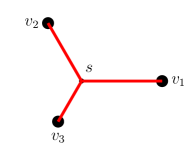
(a)  Baryons

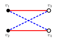
(b)  Tetraquarks: flip–flop

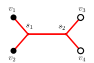
(c)  Tetraquarks: Steiner

Figure 1: Generalization of the linear quark–antiquark potential of mesons to baryons (left) and to tetraquarks, where the minimum is taken of the flip–flop (center) and Steiner tree (right) configurations.

The four-body problem in quantum mechanics is notoriously difficult. For instance, Wheeler proposed in 1945 the existence of a positronium molecule $(\rm e^{+},e^{+},e^{-},e^{-})$ which is stable in the limit where internal annihilation is neglected, i.e., lies below its threshold for dissociation into two positronium atoms. In 1946, Ore published a four-body calculation of this system PhysRev.70.90 and concluded that his investigation “counsels against the assumption that clusters of this (or even of higher) complexity can be formed”. However, in 1947, Hylleraas and the same Ore published an elegant analytic proof that this molecule is stable PhysRev.71.493 . It has been discovered recently 2007Natur.449..195C .

Similarly, the above model (2), in its linear version, was considered by Carlson and Pandharipande, who entitled their paper Carlson:1991zt “Absence of exotics in the flux tube model”, i.e., did not find stable tetraquarks. However, Vijande et al. Vijande:2007ix used a more systematic variational expansion of the wave function and in their numerical solution of the four-body problem found a stable tetraquark ground state. Moreover, unlike Carlson:1991zt , they considered the possibility of unequal masses, and found that stability improves if the quarks are heavier (or lighter) than the antiquarks, in agreement with previous investigations (see, e.g., Vijande:2007ix for Refs.).

It is thus desirable to check whether this minimal-path model supports or not bound states. The present attempt is based on an upper bound on the potential, which leads to an exactly solvable four-body Hamiltonian.

With the Jacobi vector coordinates

$$x=v_{2}-v_{1}~{},\quad y=v_{4}-v_{3}~{},\quad z=\frac{v_{3}+v_{4}-v_{1}-v_{2}}{2}~{},$$ (3)

and their conjugate momenta, the relative motion is described by the Hamiltonian

$$H=\frac{p_{x}^{2}}{M}+\frac{p_{y}^{2}}{m}+\frac{p_{z}^{2}}{4\mu}+U(x,y,z)~{},$$ (4)

where $\mu$, given by $\mu^{-1}=m^{-1}+M^{-1}$, is the quark–antiquark reduced mass. Using the scaling properties of $H$, one can set $m=1$ without loss of generality.

The simplest bound on the potential $U$ is

$$U\leq V_{4}\leq\|x\|+\|y\|+\|z\|~{},$$ (5)

as the tree with optimized Steiner points $s_{1}$ and $s_{2}$ is shorter than if the junctions are set at the middles of the quark separation $v_{1}v_{2}$ and antiquark separation $v_{3}v_{4}$. This leads to a separable upper bound for the Hamiltonian

$$H\leq H^{\prime}=\frac{p_{x}^{2}}{M}+\|x\|+p_{y}^{2}+\|y\|+\frac{p_{z}^{2}}{4\mu}+\|z\|~{}.$$ (6)

Now, the ground state $e_{0}$ of $p_{x}^{2}+\|x\|$ corresponds to the radial equation $-u^{\prime\prime}(r)+ru(r)=e_{0}u(r)$ with $u(0)=u(\infty)=0$ and is the negative of the first zero of the Airy function, $e_{0}=2.3381\ldots$ By scaling, the ground state of $\alpha p_{x}^{2}+\beta\|x\|$, with $\alpha>0$ and $\beta>0$ is $\alpha^{1/3}\beta^{2/3}e_{0}$. Thus the lowest eigenvalue of $H^{\prime}$ is

$$E^{\prime}=e_{0}\left[M^{-1/3}+1+(4\mu)^{-1/3}\right]~{},$$ (7)

with $\mu=M/(1+M)$. By comparison, the threshold of $(QQ\bar{q}\bar{q})$ is made of two identical $(Q\bar{q})$ mesons, each governed by the Hamiltonian $h=p^{2}/(2\mu)+\|r\|$, where $p$ is conjugate to the quark–antiquark separation $r$. Thus the threshold energy is

$$E_{\text{th}}=2\,e_{0}(2\mu)^{-1/3}~{},$$ (8)

and it is easily seen that $E^{\prime}>E_{\text{th}}$ for any value of the quark-to-antiquark mass ratio $M$, i.e., the bound (5) cannot demonstrate binding.

A better bound will be proved below. If there is a genuine Steiner tree linking the quarks to the antiquarks, then

$$V_{4}\leq\frac{\sqrt{3}}{2}\left(\|x\|+\|y\|\right)+\|z\|~{}.$$ (9)

But if $V_{4}$ is not associated to a genuine Steiner tree, this inequality is often violated. Consider for instance a rectangular configuration with $||v_{1}v_{2}||=||v_{3}v_{4}||\gg||v_{1}v_{3}||=||v_{2}v_{4}||$ (in this case the mathematical Steiner tree problem would require a Steiner point linking $v_{1}$ and $v_{3}$, another Steiner point linking $v_{2}$ and $v_{4}$, but the corresponding fluxes are not permitted by the color coupling in QCD), then $\|z\|\sim 0$ and $V_{4}\sim\|x\|+\|y\|$, so (9) does not hold.

However, it will be shown that

$$U\leq\frac{\sqrt{3}}{2}\left(\|x\|+\|y\|\right)+\|z\|~{},$$ (10)

for any configuration of the quarks and antiquarks, i.e., for any $x$, $y$ and $z$. Then the ground state of $H$ is bounded as

$$E<E^{\prime\prime}=e_{0}\left[\left(\frac{3}{4}\right)^{1/3}\!\left(M^{-1/3}+1\right)+(4\mu)^{-1/3}\right]~{},$$ (11)

As shown in Fig. 2, this bound $E^{\prime\prime}$ significantly improves the previous one, $E^{\prime}$. It is easily seen than $E^{\prime\prime}$ becomes smaller than $E_{\text{th}}$ for very large values of the mass ratio, more precisely for $M>6402$, and thus that the tetraquark is bound at least in this range of $M$. The numerical estimate of Vijande:2007ix actually indicates stability for all values of $M$, even $M=1$.

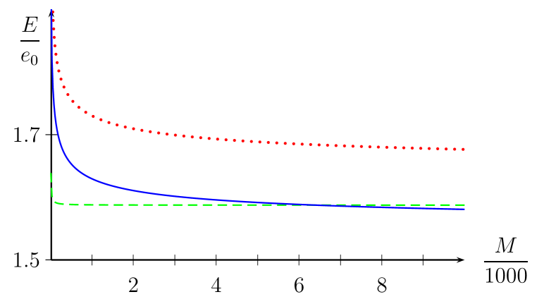
Figure 2: Simple bound $E^{\prime}$ (Eq. (7), dotted line) and improved upper bound $E^{\prime\prime}$ (Eq. (11),solid line) on the tetraquark ground-state energy as a function of quark-to-antiquark mass ratio $M$. Also shown is the threshold energy $E_{\text{th}}$ (Eq. 8), dashed line). The energies are in units of $e_{0}$, the ground state of $-\Delta+\|r\|$.

To summarize, we obtained an analytic upper bound on the ground state energy of tetraquarks systems with two units of open flavor, $(QQ\bar{q}\bar{q})$, using a model of linear confinement inspired by the strong-coupling regime of QCD. The key is an inequality on the length of a Steiner tree with four terminals. The bound confirms a recent numerical investigation, in which this potential was shown to bind these tetraquarks below the threshold for dissociation into two mesons. It remains to investigate whether this stability survives refinements in the dynamics, such as short range corrections, spin-dependent forces, etc.

It is our intention to extend this investigation to the case of the pentaquark (one antiquark and four quarks) and hexaquark configurations (six quarks), which have been much debated in recent years.

Appendix: Results on the Steiner problem

Before deriving Eq. (10), let us review some basic properties of the string potentials $V_{3}$ and $V_{4}$.

Three terminals

The three-point problem is very much documented in textbooks Coxeter:100457 ; Courant:397053 ; Hwang:1992 ; Proemel:2002 ; 0842.90116 . Let $v_{1}v_{2}v_{3}$ be the triangle, with side lengths $a_{1}=||v_{2}v_{3}||$, … and angles $\alpha_{1}=\angle{v_{1}v_{2}v_{3}}$, etc. The problem of finding a path of minimal length $\|sv_{1}\|+\|sv_{2}\|+\|sv_{3}\|$ linking the three vertices has been solved by Fermat and Torricelli. See, e.g., Coxeter:100457 . The result is the following: if one of the angles, say $\alpha_{1}$, is larger than $120^{\circ}$, $s$ coincides with $v_{1}$, otherwise each side of the triangle is seen from $s$ with an angle of $120^{\circ}$. The Steiner point $s$ is thus at the intersection of three arcs of circles, see Fig. 3.

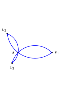
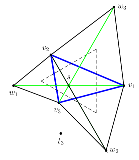
(a)

Figure 3: Left: the junction lies on each arc from which a side is seen under $120^{\circ}$. Right: the three-terminal Steiner problem as a side product of Napoleon’s theorem

The three-terminal problem is also linked to Napoleon’s theorem, which states that if one draws external equilateral triangles on each side, $v_{1}v_{2}w_{3}$, $v_{1}v_{3}w_{1}$ and $v_{1}v_{1}w_{2}$, the centers of these triangles form an equilateral triangle (dashed lines in Fig. 3(a)), a nice example of symmetry restoration. The junction $s$ is just the intersection of $v_{1}w_{1}$, $v_{1}w_{2}$ and $v_{3}$. Note that $\|sv_{1}\|+\|sv_{2}\|=\|sw_{3}\|$, and similar relations, and thus the potential is simply $V_{3}=\|v_{1}w_{1}\|=\|v_{2}w_{2}\|=\|v_{3}w_{3}\|$.

The point $w_{3}$ and its symmetric with respect to $v_{1}v_{2}$, $t_{3}$ form the toroidal domain associated to the subset $\{v_{1},v_{2}\}$. The length of the minimal Steiner tree is the maximal distance between $v_{3}$ and the domain $\{w_{3},t_{3}\}$.

From the above properties, one can estimate the string potential in a closed form. If $\alpha_{1}\geq 120^{\circ}$, then $V_{3}=a_{2}+a_{3}$, and similarly for large $\alpha_{2}$ or $\alpha_{3}$. Otherwise, $V_{3}=\sum\ell_{i}$, where $\ell_{i}=\|sv_{i}\|$. From $\hat{s}=120^{\circ}$ in the triangle $sv_{2}v_{3}$, $a_{1}^{2}=\ell_{2}^{2}+\ell_{3}^{2}+\ell_{2}\ell_{3}$, and by summation

$$2(\ell_{1}^{2}+\ell_{2}^{2}+\ell_{3}^{2})+(\ell_{1}\ell_{2}+\ell_{2}\ell_{3}+\ell_{3}\ell_{1})=a_{1}^{2}+a_{2}^{2}+a_{3}^{2}~{}.$$ (12)

Now, $\ell_{1}\ell_{2}$ being four times the area of the $sv_{1}v_{2}$ triangle, the second term in the above equation is four times the whole area of $v_{1}v_{2}v_{3}$, which is given by the Henon theorem. Altogether, in the case of a genuine Steiner tree Takahashi:2000te

$$V_{3}=\ell_{1}+\ell_{2}+\ell_{3}=\sqrt{a_{1}^{2}+a_{2}^{2}+a_{3}^{2}+\sqrt{3(a_{1}+a_{2}+a_{3})(a_{1}+a_{2}-a_{3})(a_{1}-a_{2}+a_{3})(-a_{1}+a_{2}+a_{3})}}~{},$$ (13)

which can be computed quickly.

The planar tetraquark problem.

For the four-point problem, there are many special cases, which can be treated by inspection. If, for instance the quark $v_{2}$ is on the back of $v_{1}$, as in Fig. 4(a), the problem reduces to the Steiner problem for $\{v_{1},v_{3},v_{4}\}$. Another special case is shown in Fig. 4(b), where the quarks are close to the antiquarks. For the standard Steiner problem of geometry, the solution would correspond to the Steiner tree shown as a dotted line, with a Steiner point $s_{3}$ linked to $v_{1}$ and $v_{3}$ and another one, $s_{4}$, linked to $v_{2}$ and $v_{4}$. This is not allowed by the different color properties of quarks and antiquarks, hence our best tree, shown as a solid line, has only one junction. But in estimating the potential $U$ of Eq. (2) for this configuration, the minimum is the flip–flop term $d_{13}+d_{24}$.

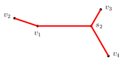
(a)  Large angle in $v_{1}$

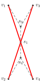
(b)  Elongated rectangle

Figure 4: Examples of special configurations. Left: one junction coincides with $v_{1}$. Right: the two junctions merge (the dotted gray line corresponds to the Steiner tree if the four points $v_{i}$ play the same role, unlike the tetraquark problem with quarks and antiquarks having conjugate colors. )

Let us turn to the case of a genuine Steiner tree $(v_{1}v_{2})s_{1}s_{2}(v_{3}v_{4})$ as in Fig. 5.

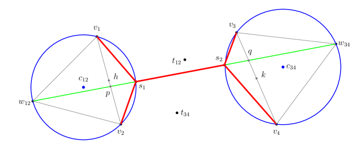
Figure 5: Construction of the minimal string in the planar case.

The string of Fig. 1(c) is minimized with respect to $s_{1}$ and $s_{2}$. Hence for fixed $s_{2}$, it assumes the Fermat–Torricelli minimization of $v_{1}v_{2}s_{1}$, a well-known iteration property of Steiner trees. Hence $\angle{v_{1}s_{1}v_{2}}=120^{\circ}$ and $v_{1}v_{2}$ is the bissector of $\angle{v_{1}s_{1}v_{2}}$ and passes through the point $w_{12}$ which completes an equilateral triangle $v_{1}v_{2}w_{12}$ in the quark sector. Similarly, it also passes through $w_{34}$ which makes $v_{3}v_{4}w_{34}$ equilateral in the antiquark sector.

The junction points $s_{1}$ and $s_{2}$ are just the other intersections of the straight line $w_{12}w_{34}$ with the circumcircles of $v_{1}v_{2}w_{12}$ and $v_{3}v_{4}w_{34}$, as shown in Fig. 5. There is a possible ambiguity about on which side $s_{1}$ or $s_{2}$ should be, but this is easily solved by the requirement that the total length of the string is minimum. Crucial is the observation that $V=\|w_{12}w_{34}\|$, so that the determination of the Steiner points $s_{1}$ and $s_{2}$ is not required to compute $V_{4}$.

A variant is that is $t_{12}$ is the symmetric of $w_{12}$ with respect to $v_{1}v_{2}$, the set $\{w_{12}t_{12}\}$ is the toroidal domain associated to the quarks, and similarly $\{w_{34}t_{34}\}$ for the antiquarks, the length of the Steiner trees is the maximal distance between these two sets.

This construction, which is a special case of the Melzak’s algorithm 0101.13201 , leads to a very easy computation. If each vector $v_{i}$ is identified with its affix (complex number) $v_{i}$, etc., then those of $w_{12}$ and $w_{34}$ are easily deduced, for instance $w_{12}=-j^{2}v_{1}-jv_{2}$ or $-jv_{1}-j^{2}v_{2}$ (depending on which side is $w_{12}$), if one uses the familiar root of unity $j=\exp(2i\pi/3)$. Once $w_{12}$ and $w_{34}$ are determined, $V=\|w_{12}w_{34}\|$. If one wishes to locate the Steiner points, it is sufficient to remark that $w_{12}s_{2}.w_{12}w_{34}=\|w_{12}c_{34}\|^{2}-r_{34}^{2}$ and $w_{34}s_{1}.w_{34}w_{12}=\|w_{34}c_{12}\|^{2}-r_{12}^{2}$, where $c_{12}$ is the center of the circle $v_{1}v_{2}w_{12}$ and $r_{12}=d_{12}\sqrt{3}/2$ its radius and $c_{34}$ and $r_{34}$ are defined similarly in the antiquark sector.

The spatial tetraquark problem

In general, the four constituents do not belong to the same plane. The minimum is achieved for $v_{1}v_{2}s_{1}s_{2}$ coplanar, and $v_{3}v_{4}s_{1}s_{2}$ also coplanar, but in a different plane. The toroidal domain to which the point $w_{12}$ belongs is the Melzak circle, of axis $v_{1}v_{2}$ and radius $r_{12}=\|v_{1}v_{2}\|\sqrt{3}/2$, and similarly for $w_{34}$ in the antiquark sector. The straight line $w_{12}w_{34}$ has to intersect these two circles as well as the lines $v_{1}v_{2}$ and $v_{3}v_{4}$. The problem consists of constructing such a straight line.

The reasoning can be made on Fig. 5, if one imagines that $v_{3}v_{4}s_{2}$ is not coplanar to $v_{1}v_{2}s_{1}$. As stressed in Rubinstein:2002 , the key is to determine $p$ and $q$, the intersections of $s_{1}s_{2}$ with $v_{1}v_{2}$ and $v_{3}v_{4}$, respectively. In this paper, the following coupled equations are derived

$$x_{p}={m\sqrt{h^{2}+x_{q}^{2}\sin^{2}\phi}+r_{12}v\cos\phi\over r_{34}+\sqrt{h^{2}+x_{q}^{2}\sin^{2}\phi}}~{},\quad x_{q}={n\sqrt{h^{2}+x_{p}^{2}\sin^{2}\phi}+r_{34}v\cos\phi\over r_{12}+\sqrt{h^{2}+x_{p}^{2}\sin^{2}\phi}}~{},$$ (14)

for the abscissa $x_{p}$ of $p$ along $v_{1}v_{2}$ and $x_{q}$ of $q$ along $v_{3}v_{4}$. These abscissas are from the common perpendicular $uv$ to $v_{1}v_{2}$ and $v_{3}v_{4}$ ($u\in v_{1}v_{2}$and $v\in v_{3}v_{4}$), with $\|uv\|=h$, $\|uh\|=m$ and $\|vk\|=n$, where $h$ is the middle of $v_{1}v_{2}$ and $k$ that of $v_{3}v_{4}$. The equations (14) can be solved by iterations, with remarkably fast convergence. Once $x_{p}$ and $x_{q}$, i.e., $p$ and $q$, are determined, the Steiner points are determined by imposing they are on the circles $v_{1}v_{2}w_{12}$ and $v_{3}v_{4}w_{34}$, respectively. For instance, if $s_{1}=p+t(q-p)$, $t$ obeys a second order equation.

If one is interested only in the length of the Steiner tree and not in the position of the Steiner points, an alternative formalism consists of locating $p$ through $p=h+x\,(v_{2}-h)$ and $q=k+y\,(v_{4}-k)$. With this notation, the length of the tree is simply

$$V_{4}=\min_{x,y}\left[\|pq\|+{r_{ab}\over\sqrt{3}}\sqrt{3+x^{2}}+{r_{cd}\over\sqrt{3}}\sqrt{3+y^{2}}\right]~{},$$ (15)

which is easily minimized by varying $x$ and $y$. The minimisation is equivalent to solving the coupled equations

$$x=\sqrt{3+x^{2}}{{v_{1}v_{2}}.{pq}\over\|v_{1}v_{2}\|\,\|pq\|}~{},\quad y=\sqrt{3+y^{2}}{{v_{3}v_{4}}.{qp}\over\|v_{3}v_{4}\|\,\|pq\|}~{},$$ (16)

which expresses that $w_{12}$, $p$, $s_{1}$, $s_{2}$, $q$ and $w_{34}$ are collinear. These equations are easily solved by iteration or any other means.

We believe that, besides checking the particular cases with large angles or a single Steiner point, the fastest computation of the connected four-quark potential consists of minimising (15) or solving (16). We expect a dramatic improvement in computing time from the above algorithm.

However, it is aesthetically appealing to attempt a further reduction of the number of variables to be determined numerically, and to provide an almost analytic estimate of the interaction as a function of the coordinates of the quarks and antiquarks. Finding $V_{4}=\|w_{12}w_{34}\|$, the maximal distance between the Melzak circles $\mathcal{C}_{12}$ and $\mathcal{C}_{34}$, is very similar to the problem of the minimal distance beween two circles in space, as addressed e.g., in 106259 ; Eberly . Neff 106259 has shown that with the help of Lagrange multipliers and Gröbner type of elimination performed by computer-algebra sofware, the squared stationary distance $V_{4}^{2}$ obeys an eighth-order polynomial equation whose coefficients are rational functions of the coordinates of $v_{1}$, $v_{2}$, $v_{3}$ and $v_{4}$.

Eberly Eberly showed that if $m$ is associated to an angle $\theta$ along $\mathcal{C}_{12}$, and $n$ to $\phi$ along $\mathcal{C}_{34}$, then imposing $\|mn\|^{2}$ to be stationary, results in two equations of the type

$$\alpha_{i}\cos\theta+\beta_{i}\sin\theta+\gamma_{i}=0~{},\qquad i=1,2~{},$$ (17)

where $\alpha_{i}$, $\beta_{i}$ and $\gamma_{i}$ contain constants and terms linear in $\cos\phi$ and $\sin\phi$. Solving (17) as two linear equations, as if $\cos\theta$ and $\sin\theta$ were independent, and then imposing $\cos\theta^{2}+\sin\theta^{2}=1$ gives an equation for $\cos\phi$ and $\sin\phi$, which is transformed into an 8^th order equation in $\cos\phi$.

It is slightly faster to rewrite (17) using $t=\tan(\theta/2)$ and $u=\tan(\phi/2)$ as

$$\delta_{i}t^{2}+\eta_{i}t+\epsilon_{i}=0~{},\qquad i=1,2~{},$$ (18)

where the coefficients are quadratic in $u$. The compatibility of two such equations is simply

$$W(\delta,\eta)W(\eta,\epsilon)=W(\delta,\epsilon)^{2}~{},\qquad W(x,y)=x_{1}y_{2}-x_{2}y_{1}~{},$$ (19)

and is directly a polynomial in $u$, of order 8.

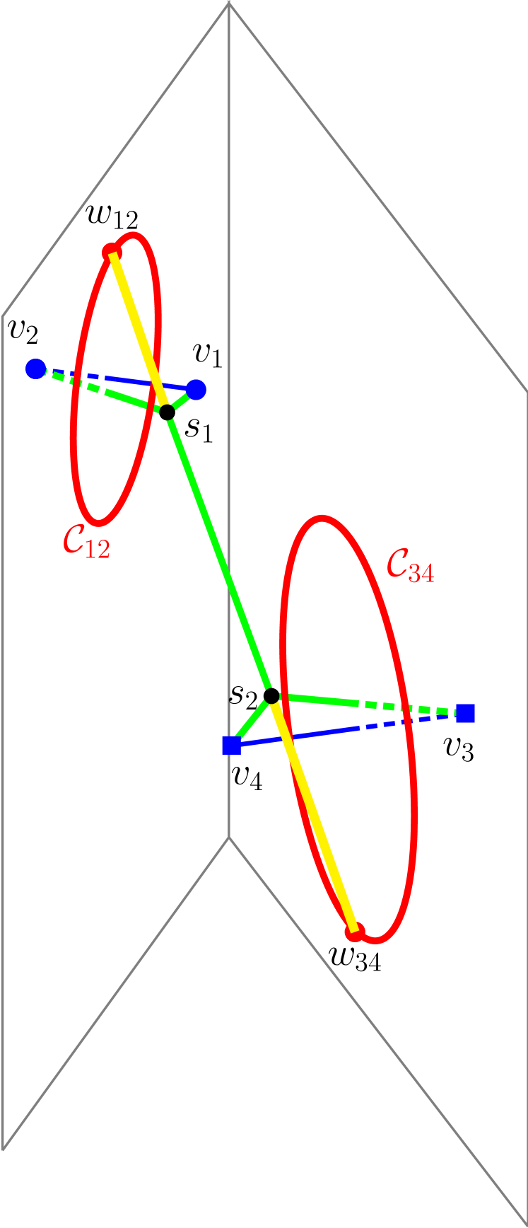
Figure 6: The confining potential $V_{4}$ for the tetraquark system $(v_{1}v_{2}v_{3}v_{4})$ is the minimal length of the tree $\|v_{1}s_{1}\|+\|v_{2}s_{1}\|+\|s_{1}s_{2}\|+\|s_{2}v_{3}\|+\|s_{2}v_{4}\|$ when $s_{1}$ and $s_{2}$ are varied. It is also the maximal distances between the circles $\mathcal{C}_{12}$ and $\mathcal{C}_{34}$, i.e., the distance $w_{12}w_{34}$. The Melzak circle $\mathcal{C}_{12}$ is centered at the middle of $v_{1}$ and $v_{2}$, has $v_{1}v_{2}$ as axis and a radius $\|v_{1}v_{2}\|\sqrt{3}/2$, and $\mathcal{C}_{34}$ has analogous properties in the antiquark sector.

Proof of the inequality (10)

If we have a positively oriented edge from $s_{1}$ to $s_{2}$, i.e., the Steiner tree is non degenerate, then we have

$$V_{4}\leq(\|x\|+\|y\|){\sqrt{3}}/2+\|z\|=B$$

using Melzak circles.

However the bound required is for $U=$ min $\{d_{13}+d_{24},d_{14}+d_{23},V_{4}\}$. So we want to confirm that

$$U\leq(\|x\|+\|y\|){\sqrt{3}}/2+\|z\|=B$$

is valid, regardless of whether $V_{4}$ is a degenerate or non degenerate Steiner tree.

We follow the variational method introduced in 0734.05040 . The problem is formulated as a global optimisation problem as follows;

Define $L$ as the length of the formal Steiner tree spanned by the four vertices. This length is obtained from the distance between the farthest points on the two Melzak circles. In terms of the usual Steiner tree components, $L=\|v_{1}s_{1}\|+\|v_{2}s_{1}\|\pm\|s_{1}s_{2}\|+\|v_{3}s_{2}\|+\|v_{4}s_{2}\|$). We get the positive sign for $\|s_{1}s_{2}\|$ if there is a real Steiner tree. On the other hand, if the Steiner vertices have interchanged position, so that on the line between the two farthest Melzak points, $s_{2}$ is closer to the Melzak point for $v_{1},v_{2}$ than $s_{1}$, then we have the negative sign for $\|s_{1}s_{2}\|$. So we can construct a formal tree on the six vertices $v_{1},v_{2},v_{3},v_{4},s_{1},s_{2}$ where the edge joining the two Steiner vertices is ‘negatively oriented’.

Now it is easy to see that $L\leq(\|x\|+\|y\|){\sqrt{3}}/2+\|z\|$. So if $V=L$ then the desired inequality follows trivially. So we only need to consider the situation where $L<V$, i.e the Steiner tree is formal rather than a real Steiner tree. Now by the inequality above, if either of $d_{13}+d_{24},d_{14}+d_{23}$ is not larger than $L$, then clearly the required inequality follows. So we only need to consider the case when $d_{13}+d_{24}>L$ and $d_{14}+d_{23}>L$.

We can parametrise the points $v_{1}$, $v_{2}$, $v_{3}$, $v_{4}$ by the numbers $\|v_{1}s_{1}\|$, $\|v_{2}s_{1}\|$, $\pm\|s_{1}s_{2}\|$, $\|v_{3}s_{2}\|$, $\|v_{4}s_{2}\|$. (It is easy to see that these four points are determined up to rotation, translation by five parameters.) By rescaling, we can assume that the sum of these five numbers is $1$, without loss of generality for the inequality. It is easy to see that all the numbers are then bounded so the domain becomes compact. So we seek a maximum of the ratio of $R=\min\{d_{13}+d_{24},d_{14}+d_{23}\}$ and $(\|x\|+\|y\|){\sqrt{3}}/2+\|z\|=B$ over this domain.

Now suppose that we rotate the triangles $v_{1}v_{2}v_{3}$ and $v_{1}v_{2}v_{4}$ around an axis line through $v_{1}v_{2}$. Clearly we can think of one triangle as being fixed and the other as moving relative to the first one. The quantity $R$ does not change by this rotation, but obviously $B$ does. Hence a maximum of the ratio $R/B$ corresponds to a minimum for $B$ under such a rotation.

Now an elementary argument shows that such a minimum for $B$ occurs for the configuration being planar, i.e when the vertex $v_{4}$ moves into the plane of $v_{1},v_{2},v_{3}$. Now assume that some initial configuration satisfies $R/B>1$ and the Steiner tree is formal rather than real. As the triangle $v_{1}v_{2}v_{4}$ rotates around an axis line through $v_{1}v_{2}$, it is easy to see that the two Melzak circles move apart. At some intermediate point, if they cross, then we find that the Steiner tree changes from being formal to being real. At this intermediate point, it is trivial to see that $R/B<1$. But this is impossible, since we have initially $R/B>1$ and $R/B$ is increasing, since $B$ is decreasing and $R$ is fixed.

On the other hand, if the Melzak circles never intersect, then this must be true for the planar configuration. So we would have such a configuration for which the Steiner tree is still formal but $R/B>1$. It is elementary to prove that this is impossible. So this completes the argument.

References

- (1) X. Artru, Nucl. Phys. B85, 442 (1975).
- (2) P. Hasenfratz, R. R. Horgan, J. Kuti and J. M. Richard, Phys. Lett. B94, 401 (1980).
- (3) H. G. Dosch, Phys. Rev. D28, 412 (1983).
- (4) E. Bagan, J. I. Latorre, S. P. Merkurev and R. Tarrach, Phys. Lett. B158, 145 (1985).
- (5) M. Fabre De La Ripelle, Phys. Lett. B205, 97 (1988).
- (6) D. S. Kuzmenko and Y. A. Simonov, Phys. Atom. Nucl. 64, 107 (2001), [hep-ph/0010114].
- (7) T. T. Takahashi, H. Matsufuru, Y. Nemoto and H. Suganuma, Phys. Rev. Lett. 86, 18 (2001), [hep-lat/0006005].
- (8) J. M. Richard and P. Taxil, Ann. Phys. 150, 267 (1983).
- (9) J. Carlson, J. B. Kogut and V. R. Pandharipande, Phys. Rev. D27, 233 (1983).
- (10) B. Silvestre-Brac, C. Semay, I. M. Narodetskii and A. I. Veselov, Eur. Phys. J. C32, 385 (2003), [hep-ph/0309247].
- (11) F. Lenz et al., Ann. Phys. 170, 65 (1986).
- (12) H.-M. Chan et al., Phys. Lett. B76, 634 (1978).
- (13) L. Montanet, G. C. Rossi and G. Veneziano, Phys. Rept. 63, 149 (1980).
- (14) G. Martens, C. Greiner, S. Leupold and U. Mosel, Phys. Rev. D73, 096004 (2006), [hep-ph/0603100].
- (15) F. Okiharu, H. Suganuma and T. T. Takahashi, Phys. Rev. D72, 014505 (2005), [hep-lat/0412012].
- (16) H. Suganuma et al., 0802.3500.
- (17) A. Ore, Phys. Rev. 70, 90 (1946).
- (18) E. A. Hylleraas and A. Ore, Phys. Rev. 71, 493 (1947).
- (19) D. B. Cassidy and A. P. Mills, Nature 449, 195 (2007).
- (20) J. Carlson and V. R. Pandharipande, Phys. Rev. D43, 1652 (1991).
- (21) J. Vijande, A. Valcarce and J. M. Richard, Phys. Rev. D76, 114013 (2007), [0707.3996].
- (22) H. S. M. Coxeter, Introduction to geometry (Wiley, New York, NY, 1969).
- (23) R. Courant and H. Robbins, What is mathematics: an elementary approach to ideas and methods (Oxford Univ. Press, London, 1958).
- (24) F. Hwang, D. Richards and P. Winter, The Steiner tree problem (North-Holland, Amsterdam, 1992).
- (25) H. J. Prömel and A. Steger, The Steiner tree problem: a tour through graphs, algorithms, and complexity (Vieweg, Wiesbaden, 2002).
- (26) A. O. Ivanov and A. A. Tuzhilin, Minimal networks: the Steiner problem and its generalizations. (Boca Raton, FL: CRC Press. xviii, 414 p. $ 78.00 , 1994).
- (27) Z. Melzak, Can. Math. Bull. 4, 143 (1961).
- (28) J. H. Rubinstein, D. Thomas and J. Weng, Geometriae Dedicata 93, 57 (2002).
- (29) C. A. Neff, IBM J. Res. Dev. 34, 770 (1990).
- (30) Dave Eberly, www.geometrictools.com/Documentation/DistancePoint3Circle3.pdf .
- (31) J. Rubinstein and D. Thomas, Ann. Oper. Res. 33, 481 (1991).