Determining the Distance of Cyg X-3 with its X-ray Dust Scattering Halo

Abstract

Using a cross-correlation method, we study the X-ray halo of Cyg X-3. Two components of dust distributions are needed to explain the time lags derived by the cross-correlation method. Assuming the distance as 1.7 kpc for Cyg OB2 association (a richest OB association in the local Galaxy) and another uniform dust distribution, we get a distance of $7.2^{+0.3}_{-0.5}$ kpc (68$\%$ confidence level) for Cyg X-3. When using the distance estimation of Cyg OB2 as 1.38 or 1.82 kpc, the inferred distance for Cyg X-3 is $3.4^{+0.2}_{-0.2}$ or $9.3^{+0.6}_{-0.4}$ kpc respectively. The distance estimation uncertainty of Cyg X-3 is mainly related to the distance of the Cyg OB2, which may be improved in the future with high-precision astrometric measurements. The advantage of this method is that the result depends weakly on the photon energy, dust grain radius, scattering cross-section, and so on.

1 Introduction

The X-ray dust scattering halo was first discussed by Overbeck in 1965. From then on, many authors developed the theory of scattering. However, there was no direct evidence for this phenomenon until 1980s when Rolf (1983) first observed the X-ray halo by analyzing the data of GX339-4 with the imaging proportional counter (IPC) instrument onboard the Einstein X-ray Observatory. There are two groups of methods to study the X-ray scattering halo. The first is evaluating the halo surface brightness distribution around the point source. During the past quarter century, X-ray halos can be found in the data of Einstein, ROSAT, XMM-Newton, Chandra and Swift. Predehl & Schmitt (1995) analyzed the data of ROSAT and found a strong correlation between the visual extinction and the hydrogen column density of 25 point sources. Vaughan et al. (2004, 2006) found ring structures in two gamma-ray burst (GRB) observations with XMM-Newton and Swift. Smith, Edgar & Shafer (2002) reported the halo of GX 13+1 between 50^′′ and 600^′′ with the data of Advanced CCD Imaging Spectrometer (ACIS) onboard the Chandra X-ray Observatory. Yao et al. (2003) determined that the halo of Cyg X-1 is as close to the point source as 1^′′, using a reconstruction method with the data of Continuous Clocking Mode of ACIS. Xiang, Zhang & Yao (2005) reconstructed the halo’s surface brightness of 17 bright sources and deduced the dust distribution along the line of sight (LOS) with the data from ACIS-S array.

The other way is to study the effect of delay and broadening of the light curve. Tr$\mathrm{\ddot{u}}$mper & Sch$\mathrm{\ddot{o}}$nfelder (1973) first proposed to use the delay and smearing property to determine the distances of the X-ray sources. Predehl et al. (2000) first used the delay property in determining the distance of Cyg X-3 with the data of ACIS. Hu, Zhang & Li (2004) developed a method of using the power density spectra to determine the distances of X-ray sources. Xiang, Lee & Nowak (2007) used the delay property to determine the distance of 4U 1624-490. Vaughan et al. (2004, 2006) evaluated the distances of some dust molecular clouds by the delayed ring structures in two GRB observations with XMM-Newton and Swift. Thompson & Rothschild (2008) used the eclipse data determining the distance of Cen X-3 to be 5.7 $\pm$ 1.5 kpc. Ling et al. (2009) first used the cross-correlation method to study the light curves of the X-ray halo of Cyg X-1. They found obvious time lag peaks in the cross-correlation curves. All those peaks revealed a dust concentration at a distance of 1.76 kpc from us.

Actually, the first method uses the halo surface brightness distribution to study the dust distribution and dust model, whereas the second method studies the dust distribution and source distance. The goals from each type of study are usually different. Both techniques require careful point-spread function (PSF) subtraction during the analysis.

In this work, we re-analyze the data of Cyg X-3 with the cross-correlation method described in Section 2. We discuss the multiple scatterings in Section 4. After obtaining the cross-correlation curves from 15^′′ to 80^′′, we use two dust distributions to explain the time lags. Assuming the distance as 1.7 kpc for Cyg OB2 and another uniform dust distribution, we get a distance of $7.2^{+0.3}_{-0.5}$ kpc (68$\%$ confidence level) for Cyg X-3 in Section 5. When using the distance estimation of Cyg OB2 as 1.38 or 1.82 kpc, the inferred distance for Cyg X-3 is $3.4^{+0.2}_{-0.2}$ or $9.3^{+0.6}_{-0.4}$ kpc respectively. We summarize our results in Section 6.

2 Method and Data preparation

The details of X-ray dust scattering can be found in Van de Hulst (1957), Overbeck (1965), Tr$\mathrm{\ddot{u}}$mper & Sch$\mathrm{\ddot{o}}$nfelder (1973), and Smith & Dwek (1998). Here, we just show some equations used in this work.

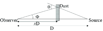
Figure 1: X-ray dust scattering geometry.

As shown in Figure 1, an X-ray source is located at a distance of $\mathit{D}$. The dimensionless number $\mathit{x}$ is the ratio of the distance of scattering and that of the source from us. So the lag time of scattered photons at $\mathit{x}$ can be expressed as

$$t_{\mathrm{Delay}}(\phi,x)=\left(\frac{x}{\cos\phi}+\sqrt{(1-x)^{2}+(x\tan\phi)^{2}}-1\right)\times\frac{D}{c}.$$ (1)

Let $\mathit{I(t)}$ denote the observed flux of the source at $x=0$, the observed halo intensity at different observational angle $\phi$ is given by

$$H(\phi,t)=\int_{0}^{1}{{\mathrm{d}x}}\times{D}\times\frac{I(t-t_{\mathrm{Delay}}(\phi,x))\times{\rho(x)}}{(1-x)^{2}}\times\frac{d\sigma(\theta)}{d\Omega},$$ (2)

where the scattering cross section $\frac{d\sigma(\theta)}{d\Omega}$ depends on the energy of the X-ray photon and the radius of the dust grain. $\rho(x)$ is the density (in units of $\mathrm{cm^{-3}}$) of the dust grain at $\mathit{x}$. If $\mathit{I(t)}$ equals to a delta function, equation 2 would evolve to be a response function of a delta function (we denote this function by $\mathit{R(\phi,t)}$ hereafter). This is the situation of a GRB, hence equation 2 would be an ideal observed light curve of a halo at a given observational angle $\mathit{\phi}$. For the other situations, the light curve of the halo at angle $\phi$ equals to the convolution of $\mathit{I(t)}$ and $\mathit{R(\phi,t)}$. This process can also be understood by Figure 1. The light curve of the halo at observational angle $\phi$ is an integral effect of scattering from the dust near the observer to the source. From this process, the light curve of the halo would be lagged and smeared from the light curve of the source.

We can study the delay property directly with the cross-correlation method (Ling et al. 2009). The definition of cross-correlation coefficient is given by

$$c(\Delta t)=\frac{1}{N-\arrowvert{\Delta t}\arrowvert}\sum_{t=0}^{N-\arrowvert{\Delta t}\arrowvert-1}(L_{h}(t+\Delta t)-\mu_{h})(L_{s}(t)-\mu_{s}),$$ (3)

here $\mathit{L_{s}}$ and $\mathit{L_{h}}$ are the light curves of the X-ray source and halo (at a given observational angle $\phi$) in the same energy band. $\mu_{s}$ and $\mu_{h}$ are the average values of $\mathit{L_{s}}$ and $\mathit{L_{h}}$ respectively.

Table 1: Observations of Cyg X-3 we used.

ObsID	Exposure (ks)	Start date	Instrument
1456	20.8	1999-10-20	ACIS-S
425	21.53	2000-04-04	ACIS-S
426	18.32	2000-04-06	ACIS-S

3 Data extraction and Result

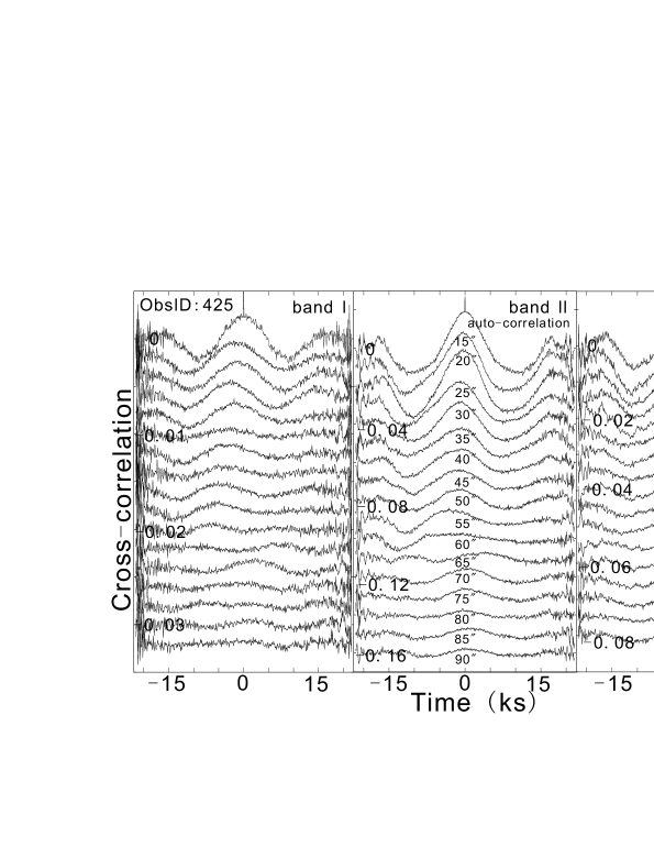
Figure 2: Cross-correlation curves of ObsID425. The top curve in each panel is the autocorrelation of the light curve of the source; all other curves are the cross-correlation curves from 15^′′ to 90^′′ with a step of 5^′′. For clarity, the cross-correlation coefficients have been lowered by a same amount successively for each curve.

Three observational data sets, listed in table 1, are used in our analysis. The CIAO version 3.4 and CALDB version 3.4.1 are used to process the observational data. The main process in this study is similar to the way described in Ling et al. (2009). Here, we just give a brief description. First, we divide the observational data into three energy bands: below 3 keV (band I), 3 keV-5 keV (band II), and above 5 keV (band III). Second, we get the light curve of the point source by the photons in the region of the streak. Third, the light curve of the halo at each bin (the bin width is 5^′′) of observational angle is obtained from the photons of different annuli around the point source. All background contributions have been excluded for all the light curves above. After extracting all light curves, we make cross-correlation curves between the light curves of the halo and the light curve of the source in Figure 2-4. The top curve in each panel is the autocorrelation of the light curve of the source; all other curves are the cross-correlation curves from 15^′′ to about 90^′′ with a step of 5^′′. For clarity, the cross-correlation coefficients have been lowered by a same amount successively for each curve. The auto-correlation curves have a peak because of the intrinsic variations of 4.8 hr of the source. The peaks of the cross-correlation curves of the halo below 50^′′ lagged a little from the center; however the peaks of 60^′′ and 65^′′ advanced ahead of the center obviously. The relationship between the lag time and the observational angle of Cyg X-3 is quite different from that of Cyg X-1 (Ling et al. 2009), of which the lag times moved longer gradually with the increasing angles. Therefore, the lag times of Cyg X-3 cannot be explained by the scattering of a single dust wall, as suggested by the data of Cyg X-1. The moving effect is not clear in band III because of the low cross section of scattering for high energy photons. Because of its low count rate, the curves of ObsID1456 show peaks less clearly than the other two observations.

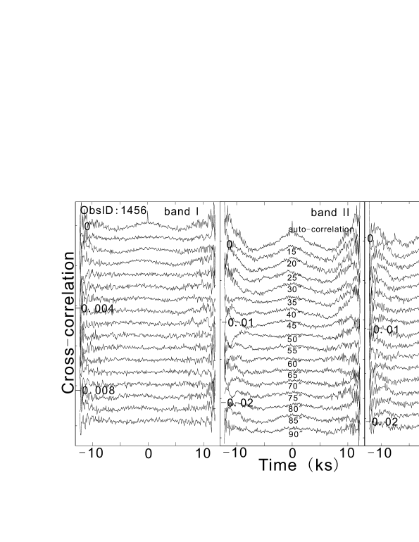
Figure 4: Cross-correlation curves of ObsID1456.

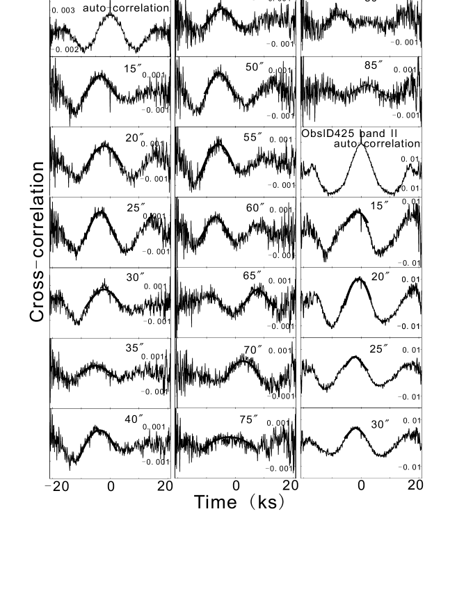
Figure 5: Cleaned cross-correlation curves used in this work. The fitting results of the peaks are shown as the solid lines, with a simple Gaussian function.

In Figure 2-4, the cross-correlation curves are contaminated by the instrument because of the PSF effect. As described in Ling et al. (2009), ChaRT and Marx are used to simulate the contaminated factor of the PSF. After obtaining those factors of contamination, we could get a cleaned cross-correlation curve. The cleaned cross-correlation curves are shown in Figure 5-8. By fitting the peaks with a simple Gaussian function, we get the time lag at each angle. The dashed lines in each panel show the fitting result of a Gaussian function. Those four figures show the result of all of the data that have obvious lag in the cross-correlation curves. We list the time lags obtained from the cross-correlation curves in Table 2. The curves of ObsID1456 have no peaks at angles greater than 50^′′ because of its lower count rate. The band I of this observation also has no peak (as can be seen in Figure 4 directly). From those figures, we find that the lag time of the cross-correlation method of band I are similar with the uncleaned cross-correlation curves of Figure 2 and 3. This also happened in the study of Cyg X-1 (Ling et al. 2009). The reason is that the PSF of the low energy band is narrower than the high energy band.

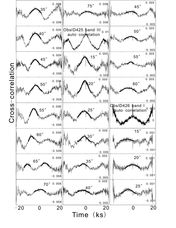
Figure 6: Fig.5 continued.

In the panel of 65^′′ in band II of ObsID425 (Figure 6, left side), there are two obvious peaks in the cleaned cross-correlation curves. The left peak with a time lag of about 10 ks and the right peak with a time lag of about $-$6 ks. The interval between those two peak is about 17 ks, which equals to the period of the light curve of source, i.e., 4.8 hr. This result confirms that the time lag derived by cross-correlation method is real but not noise. There are many other curves that show this property: from 50^′′ to 65^′′ in band II of ObsID425 and ObsID426 show two peaks. The curve of band III is not clear because the low efficiency of the scattering. Consequently, this phenomenon confirms that the time lags of 50^′′-65^′′ we derived from the cross-correlation curves are reliable. For the data of 80^′′ and 85^′′, there is only one lag time from band I of ObsID425; thus we do not use those data for further analysis in the following section.

Table 2: Time lag of cross-correlation curve (in Units of Second).

Angle	ID425	ID425	ID425	ID426	ID426	ID426	ID1456	ID1456	mean
Band	BandI	BandII	BandIII	BandI	BandII	BandIII	BandII	BandIII	-
15′′	3467	1424	975	5303	2281	1513	410	889	2032$\pm$621
20′′	2011	931	915	146	677	882	82	390	754$\pm$233
25′′	3508	2241	1548	4081	2456	2391	1109	426	2220$\pm$459
30′′	2121	1918	1483	3906	2873	2102	160	-	2080$\pm$477
35′′	5069	3028	2327	4899	3792	2956	8043	546	3833$\pm$852
40′′	3723	3840	3070	4937	4441	3617	1935	-	3652$\pm$643
45′′	4844	3402	1903	2152	5789	3116	2613	-	3403$\pm$733
50′′	5604	2839	1862	4058	3076	1657	-	-	2735$\pm$667
55′′	5866	4670	1885	4727	5046	3965	-	-	3745$\pm$616
60′′	6834	6797	4240	4930	5893	4669	-	-	4775$\pm$505
65′′	9558	10450	-	9129	9427	11617	-	-	10036$\pm$516
70′′	14617	16297	-	-	13829	15084	-	-	14957$\pm$620
75′′	19370	15961	-	-	-	18833	-	-	18055$\pm$1397
80′′	24833	-	-	-	-	-	-	-	-
85′′	32488	-	-	-	-	-	-	-	-

4 Multiple Scatterings

Before the analysis of the data of table 2, we estimate the influence of the multiple scatterings. Because of its high hydrogen column density, the multiple-scattered photons may contaminate the observed light curve of the halo. The details of multiple scatterings can be found in Mathis $\&$ Lee (1991). The conclusion in their study was that the single scattering dominates at small angles ($\theta<60^{\prime\prime}$ for $\tau_{\mathrm{sca}}=2$ at E = 1 keV).

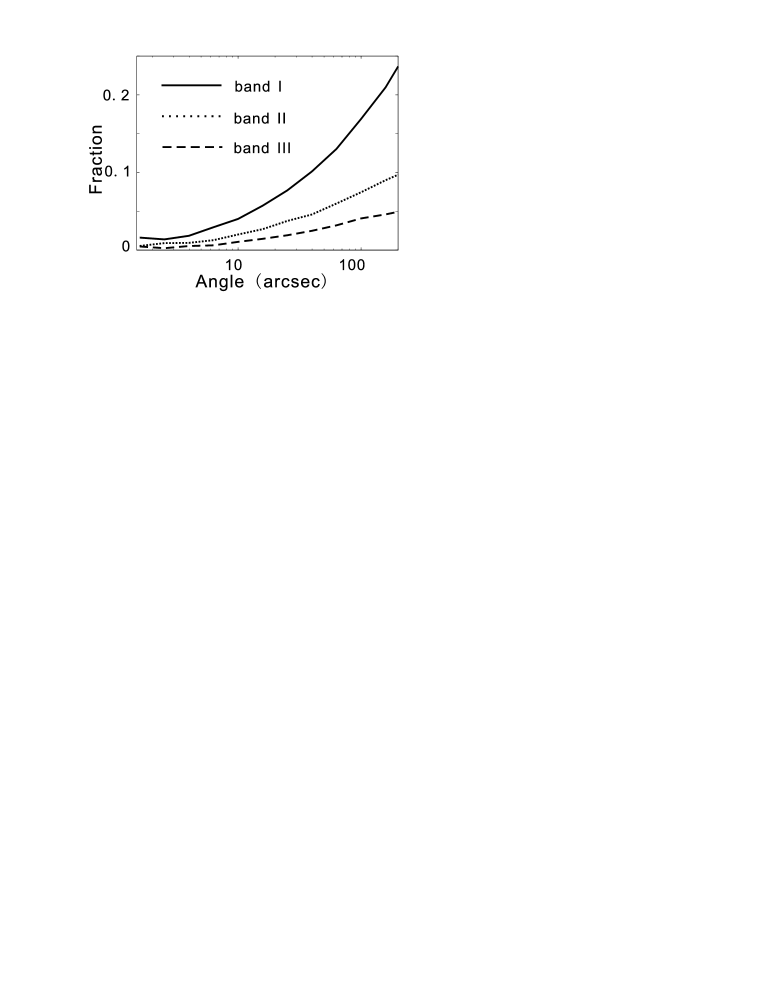
Figure 9: Simulated fractions of multiple-scattered photons to the total halo photons within each energy band as functions of the observational angle. The parameters we used are $\tau_{\mathrm{sca}}=2$ at E = 1 keV and a = 0.1 $\mu$m. The solid line shows the fraction of multiple-scattered photons for band I (below 3 keV). The dotted line shows the fraction of multiple-scattered photons for band II (3 to 5 keV). The dashed line shows the fraction of multiple-scattered photons for band III (above 5 keV).

A Monte Carlo simulation is conducted to estimate the effect of multiple scatterings. The parameters we used are $\tau_{\mathrm{sca}}=2$ at E = 1 keV and a = 0.1 $\mu$m. The simulated fractions of multiple-scattered photons to the total halo photons are shown in Figure 9. The solid line shows the fraction of multiple-scattered photons for band I (below 3 keV). The dotted line shows the fraction of multiple-scattered photons for band II (3-5 keV). The dashed line shows the fraction of multiple-scattered photons for band III (above 5 keV). From Figure 9, in band I the fraction of multiple-scattered photons is 8$\%$, 13$\%$, and 15$\%$ at observational angles of 30^′′, 60^′′, and 80^′′, respectively. Compared with the uncertainties for the lag times derived in table 2, the influence of multiple-scattered photons can be ignored in our analysis.

5 Analysis and Discussion

5.1 Uniform dust distribution

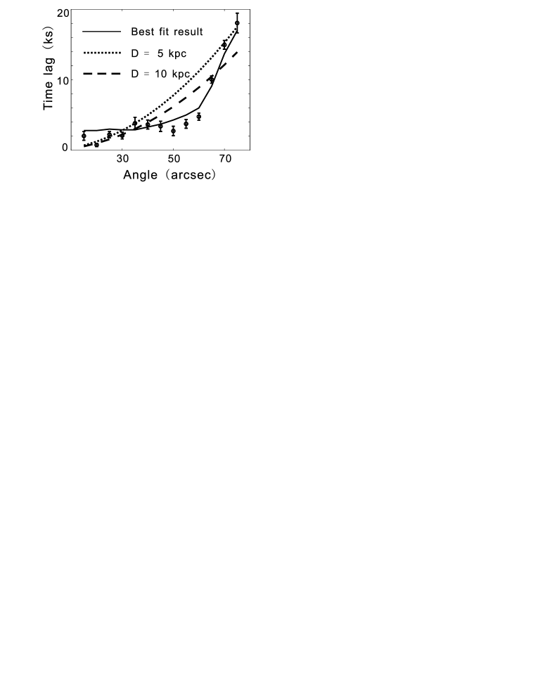
Figure 10: Observed time lag vs. observational angles. The solid line shows the best-fit result obtained in Section 4.3. The dashed line shows a model assuming a dust wall located at 1.7 kpc from the Sun and a distance of 5 kpc to the source. The dotted line shows the same model with a distance of 10 kpc to the source.

Predehl et al. (2000) analyzed the data of Cyg X-3 previously. They compared the light curve of the halo within about 10^′′ and the light curve of the point source. They found a lag of about 2 ks in the light curve directly. Assuming a uniform dust distribution, they got a distance of $9^{+4}_{-2}$ kpc for Cyg X-3. In our study, three observations are used to determine the lag time up to 75^′′. Figure 10 shows the result of lag time at each observational angle. From our result, the time lags of 60^′′-75^′′ show significant increase compared to the other time lags.

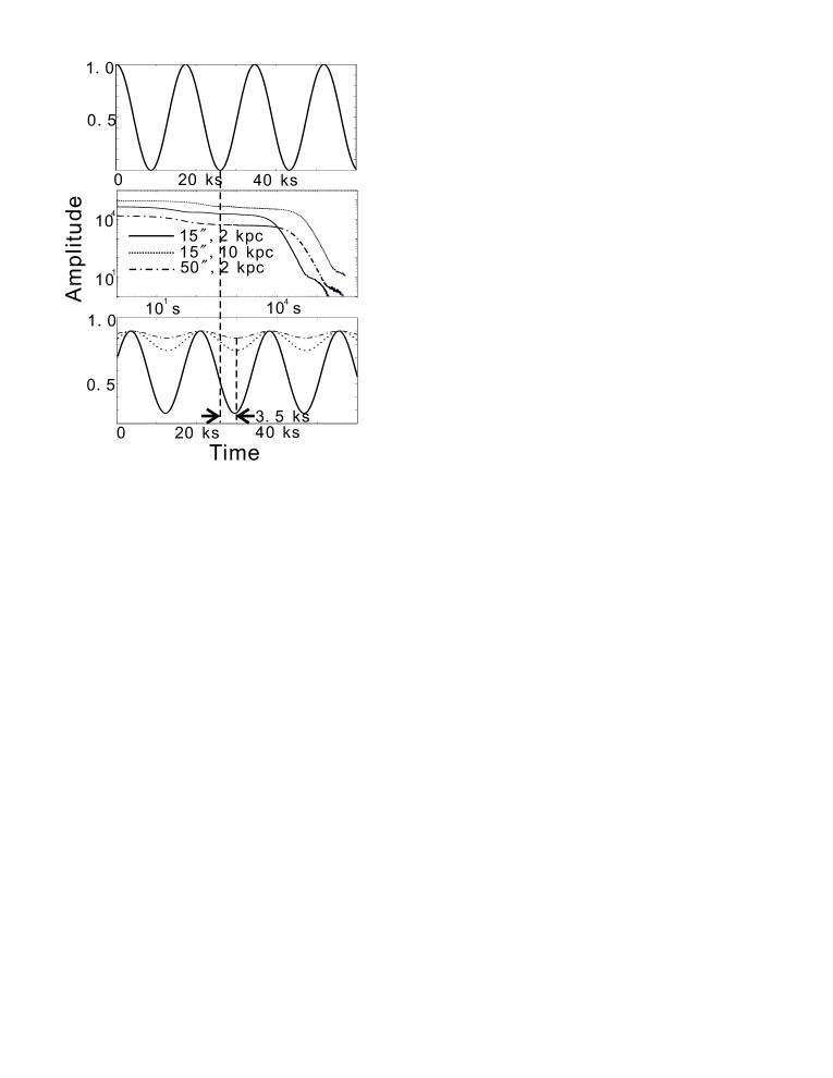
Figure 11: Convolution process with different parameters. The top panel shows a sinusoidal wave, representing the light curve of the source. The middle panel shows three curves of $\mathit{R(\phi,t)}$ in logarithm scale with a uniform dust distribution. The solid line shows the $\mathit{R(\phi,t)}$ with the parameter of $\mathit{D}=2$ kpc and $\phi=$15^′′, the dotted line shows the $\mathit{R(\phi,t)}$ of $D=10$ kpc and $\phi$ = 15^′′, and the dashed line shows the $\mathit{R(\phi,t)}$ of $D=2$ kpc and $\phi=50$^′′. The bottom panel shows the result of convolution with these three different $\mathit{R(\phi,t)}$. These three curves are treated as the light curves of halo at different observational angles. The vertical axis of the bottom panel is normalized to unity for clarity. A lag of 3.5 ks is seen in these light curves directly.

First, we try to fit the data with the same model described by Predehl et al. (2000). A uniform dust distribution is used to produce an $\mathit{R(\phi,t)}$. By convoluting the $\mathit{R(\phi,t)}$ with an ideal sinusoidal wave, we get a simulated light curve of halo at observational angle $\phi$. The dust model we used here is proposed by Mathis, Rumpl & Nordsiech 1977 (MRN hereafter). We show the process and the result in Figure 11. The top panel shows a sinusoidal wave, representing the light curve of the source. The middle panel shows three curves of $\mathit{R(\phi,t)}$ in logarithm scale. The solid line shows the $\mathit{R(\phi,t)}$ with the parameter of $\mathit{D}=2$ kpc and $\phi=$15^′′, the dotted line shows the $\mathit{R(\phi,t)}$ of $D=10$ kpc and $\phi$ = 15^′′, and the dashed line shows the $\mathit{R(\phi,t)}$ of $D=2$ kpc and $\phi=50$^′′. The bottom panel shows the result of convolution of the sinusoidal wave with these three different $\mathit{R(\phi,t)}$. These three curves are treated as the light curves of halo at different angles. The vertical axis of the bottom panel is normalized to unity for clarity. The three simulated light curves of the halo show different magnitude but have the same lag time. This result shows that if the distance of the source exceeds 2 kpc, the time lag between the light curve of the halo and that of the source will be a constant: around 3.5 ks (less than $T$/4 of the sinusoidal wave). This is also the situation for any angle larger than 15^′′. The main reason is that the profile of $\mathit{R(\phi,t)}$ is much longer than the period of the sinusoidal wave.

5.2 Single dust wall model: Cyg Ob2 association

From the discussion of Cyg X-1 (Ling et al. 2009), we found that the dust distribution is quite nonuniform toward Cyg X-1: a dust concentration at a distance of 2.0 kpc $\times$ (0.876 $\pm$ 0.002) from the Earth is found. Thus, we try to find some dust cloud around the region of Cyg X-3 to explain the time lag of 65^′′ and the greater than 65^′′.

A likely candidate for the dust concentration is the Cyg OB2 association. Cyg OB2 is one of the richest OB associations in the local Galaxy; it houses many of the hottest and most luminous stars known in our Galaxy. Cyg X-3 lies in the field of Cyg OB2 (Kn$\mathrm{\ddot{o}}$dlseder 2003). Hutchings (1981) assumed an absolute distance modulus (m$-$M) = 10.7, converting to $\mathit{d}$ = 1.38 kpc. Humphreys (1978) adopted $d$ = 1.82 kpc, while Torres-Dodgen et al. (1991) and Massey & Thompson (1991) determined $d$ = 1.74 kpc ((m - M) = 11.2). Kn$\mathrm{\ddot{o}}$dlseder (2000) assumed a distance $d=$ 1.7 kpc. In this work, a distance of 1.7 kpc for Cyg OB2 is used in the following analysis.

Assuming the distance of Cyg X-3 to be 10 kpc, the time lag of 65^′′ reveals that a dust concentration exists at a distance of about 2 kpc. This result is consistent with the distance of Cyg OB2. Then taking the distance of Cyg OB2 to be 1.7 kpc, we use a single dust wall model to fit the observed time lag. The result is shown in Figure 10, in which the dashed line shows the shows a model assuming a dust wall 1.7 kpc from the Sun and a distance of 5 kpc to the source. The dotted line shows the same model with a distance of 10 kpc to the source. Those two curves cannot fit the observed lags.

5.3 Uniform distribution plus dust wall

Combining the results of Section 5.1 and 5.2, we propose to use two components to fit the observed time lags. We divide the observed time lags into two parts: below 60^′′ and above 65^′′. The first part mainly comes from the component of a uniform dust distribution and the second part is mostly due to a dust concentration of Cyg OB2 at the distance of around 1.7 kpc, reflecting that the small angle halo tends to explore the dust near the source (Mathis $\&$ Lee 1991). The new two-components dust distribution model needs two parameters to fit the observed time lags. The first parameter is the distance $D$ of the point source and the other parameter is the fraction of the dust concentrated in Cyg OB2. The solid line of Figure 10 shows the best-fitting result. From this result, we get a distance of $7.2^{+0.3}_{-0.5}$ kpc (68$\%$ confidence level) of Cyg X-3. The fraction of dust concentrated in Cyg OB2 is $7^{+1.0}_{-0.5}\%$ (68$\%$ confidence level). The uncertainty of the distance is calculated by $\Delta\chi^{2}=2.3$ (Avni 1976). At the same time, we refit the data with the distance assumption of Cyg Ob2 to be 1.38 and 1.82 kpc away from us. The fitting results are $3.4^{+0.2}_{-0.2}$ and $9.3^{+0.6}_{-0.4}$ kpc, respectively.

Alternatively, a new way is proposed to give a range for the distance of Cyg X-3. We define the response function of a uniform dust distribution with $\mathit{R_{u}(t)}$, and the response function of the dust wall with $\mathit{R_{w}(t)}$ for simplicity. Then, the light curve of the halo is given by

$$H(t)=L(t)\otimes(R_{u}(t)+R_{w}(t)),$$ (4)

here $\otimes$ stands for convolution. Equation 4 can be decomposed to

$$H(t)=L(t)\otimes R_{u}(t)+L(t)\otimes R_{w}(t).$$ (5)

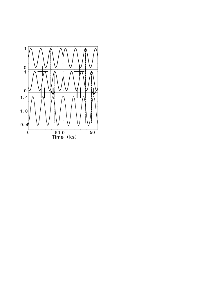
Figure 12: Illustration of the sum of two sinusoidal functions. The top panel represents the light curve of $L(t)\otimes R_{u}(t)$, the middle panel represents the light curve of $L(t)\otimes R_{w}(t)$. The left part of the middle panel has a lag of less than $T/2$ with respect to the top panel, and the right part has a lag of larger than $T/2$ with respect to the top panel. The bottom panel shows the sum of the above two panels. The arrows show the lag of the summed curves.

Equation 5 can be understood as the light curve of the halo being the sum of the two components from the two dust distributions. We use $H_{u}(t)$ and $H_{w}(t)$ hereafter to identify those two components. As pointed out in Section 5.1, the $H_{u}(t)$ may cause a lag of about 3.5 ks (of course it must also have a period of $T$, the same as the $L(t)$). The time lag of the $H_{w}(t)$ depends on the distance of Cyg X-3, but obviously $H_{w}(t)$ has a period of $T$ too. As a result, the phase of $H(t)$ is related to these two components: $H_{u}(t)$ and $H_{w}(t)$. As shown in Figure 12, the top panel represents the light curve of $L(t)\otimes R_{u}(t)$, the middle panel represents the light curve of $L(t)\otimes R_{w}(t)$. The left part of the middle panel has a lag of less than $T/2$ with respect to the top panel, and the right part has a lag of larger than $T/2$ with respect to the top panel. The bottom panel shows the sum of the above two panels. The arrows show the lag of the summed curves. The sum of those two components can cause two possible results: if

$$Lag(H_{u}(t))=3.5\ \mathrm{ks}<Lag(H_{w}(t))<12\ \mathrm{ks}=Lag(H_{u}(t))+T/2,$$ (6)

then

$$3.5\ \mathrm{ks}<Lag(H(t))<12\ \mathrm{ks},Lag(H(t))<Lag(H_{w}(t));$$ (7)

Alternatively if

$$12\ \mathrm{ks}<Lag(H_{w}(t))<12\ \mathrm{ks}+T/2,$$ (8)

then

$$12\ \mathrm{ks}<Lag(H(t))<12\ \mathrm{ks}+T/2,Lag(H(t))>Lag(H_{w}(t)).$$ (9)

The first situation means that when the lag time of $H_{w}(t)$ is less than the time lag of $H_{u}(t)$ plus $T$/2, i.e., about 12 ks, the time lag of $H(t)$ will be between 3.5 and 12 ks. The second case means that if the time lag of $H_{w}(t)$ is between 12 and 20.5 ks, the time lag of the summed curve will be greater than the time lag of $H_{w}(t)$. In other words, the second situation means that the observed time lag of the halo could be longer than the time lag caused by the dust wall.

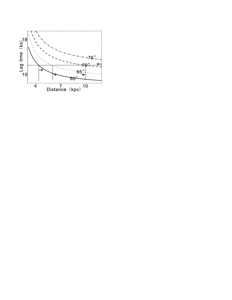
Figure 13: Geometrical lag time caused by the dust wall distribution as a function of the distance of the point source. The distance of dust wall is assumed to be 1.7 kpc for all cases. The solid line shows the lag time at 60^′′, the dotted line shows the lag time at 65^′′, the dashed line shows the lag time at 70^′′, and the dashed dotted line shows the lag time at 75^′′. The four arrows indicate the distance upper or lower limits from those four angles. Finally, a distance range of [6, 10] kpc is obtained for Cyg X-3.

Let us apply these results to the observed time lags of Figure 10. The time lag at 65^′′ is around 10 ks, less than 12 ks. Therefore, the time lag of $H_{w}(t)$ must be less than 12 ks, as we illustrated in Figure 13. In Figure 13, the solid line is the lag time at 60^′′, the dotted line is the lag time at 65^′′, the dashed line is the lag time at 70^′′, and the dashed dotted line is the lag time at 75^′′. With the constraint of 12 ks, the distance of the source must be greater than 4.5 and 6 kpc by the data of 60^′′ and 65^′′. The maximum of the distance can be derived by the data of 70^′′, of which the time lag of the dust wall must exceed 20.5 ks; a distance upper limit of 10 kpc is derived at this angle. The time lag of 75^′′ would give an upper limit of 15 kpc. Using all these result, we give a range of [6, 10] kpc for Cyg X-3. The best-fit result of $7.2^{+0.3}_{-0.5}$ kpc is among this range obviously.

5.4 Halo surface brightness of Cyg X-3

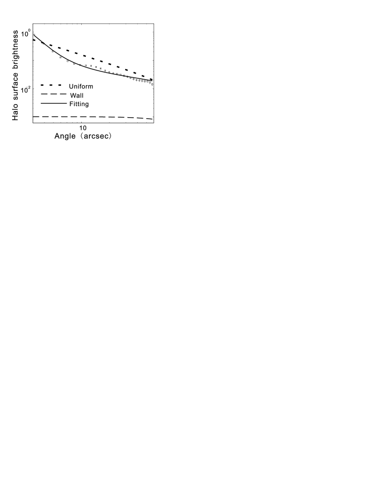
Figure 14: Halo surface brightness of Cyg X-3. The dotted line shows the predicted surface brightness of a uniform distribution, and the dashed line shows the predicted surface brightness caused by Cyg OB2. The total $\mathit{N_{H}}$ used here is $3.0\times 10^{22}$ $\mathrm{cm^{-2}}$, and the fraction of the dust existing in Cyg OB2 is 7$\%$, according to the result obtained with the cross-correlation method. The solid line shows the fitting result of a three-components dust distribution. The column density $\mathit{N_{H}}$ of the uniform distribution, the dust wall and the dust near the source (at x $>$ 0.99) are 7.0 $\pm$ 0.3 $\times 10^{21}$ $\mathrm{cm^{-2}}$, 32.0 $\pm$ 1.7 $\times 10^{21}$ $\mathrm{cm^{-2}}$ and 3.04 $\pm$ 0.06 $\times 10^{21}$ $\mathrm{cm^{-2}}$, respectively. The total $\mathit{N_{H}}$ from the fitting is consistent with the result of Predehl and Schmitt (1995).

After obtaining the ratio between the two dust components, we can predict a halo surface brightness distribution with a dust grain model. We find that the halo surface brightness distribution predicted by the MRN dust model and the two-components dust distribution cannot fit the observed halo surface brightness derived in Xiang, Zhang & Yao (2005). In Figure 14, the dotted line shows the predicted surface brightness of a uniform distribution, and the dashed line shows the predicted surface brightness caused by Cyg OB2. The total $\mathit{N_{H}}$ used here is $3.0\times 10^{22}$ $\mathrm{cm^{-2}}$ (the $\mathit{N_{H}}$ derived by Predehl and Schmitt (1995) is $3.31\times 10^{22}$ $\mathrm{cm^{-2}}$), and the fraction of the dust in Cygnus OB2 is 7$\%$; clearly the dust wall has almost no influence on the halo surface brightness. The predicted halo surface brightness of source cannot fit the observed surface brightness of Cyg X-3 obviously. Similar discrepancy has been found in our previous work on Cyg X-1 (Ling et al. 2009). To fit the halo surface brightness of angles smaller than 10^′′, we add a new dust component between x = 0.99 and x = 1.0. The fitting result is shown by the solid line in Figure 14. The column density $\mathit{N_{H}}$ of the uniform distribution, the dust wall and the dust near the source are 7.0 $\pm$ 0.3 $\times 10^{21}$ $\mathrm{cm^{-2}}$, 32.0 $\pm$ 1.7 $\times 10^{21}$ $\mathrm{cm^{-2}}$ and 3.04 $\pm$ 0.06 $\times 10^{21}$ $\mathrm{cm^{-2}}$ respectively. The total $\mathit{N_{H}}$ from the fitting is consistent with the result of Predehl and Schmitt (1995). Our fitting shows that the ratio of $N_{H}$ in the dust wall to the $N_{H}$ of the uniform dust distribution is 4.6, conflicting significantly from our result of 0.075 derived with the cross-correlation method which is almost independent of the dust size distribution model. As a result, we conclude that the MRN dust model must be modified before it is used in the X-ray regime.

5.5 Independence of dust grain model

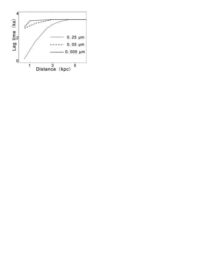
Figure 15: Lag time of $H_{u}(t)$ of 15^′′ vs. the distance of the source. The solid line shows the lag time of $H_{u}(t)$ with a dust radius of 0.005 $\mu$m, the dashed line shows the lag time of $H_{u}(t)$ with a dust radius of 0.05 $\mu$m, and the dotted line shows the lag time of $H_{u}(t)$ with a dust radius of 0.25 $\mu$m. The lag time approaches to 3.5 ks when the distance of the source exceeds 5 kpc for any dust radius.

In Section 5.4, we have shown that the MRN model is not sufficient in modeling the halo surface brightness distribution along the LOS of Cyg X-3. However, in the analysis of Section 5.1, the MRN dust grain model was used to produce $R_{u}(t)$, the response function of a uniform dust distribution. Here, we address the question whether our result is dependent of the dust grain model. From equation 2, we can get $R_{u}(t)$ with different dust radii directly. Then, we could get a simulated $H_{u}(t)$ for any dust radius. After comparing the phase of the light curve of source and $H_{u}(t)$, we get the lag time in different dust radii. Figure 15 shows the lag time of $H_{u}(t)$ of 15^′′ versus the distance of the source. The solid line represents the lag time of $H_{u}(t)$ with a dust radius of 0.005 $\mu$m, the dashed line represents the lag time of $H_{u}(t)$ with a dust radius of 0.05 $\mu$m, and the dotted line represents the lag time of $H_{u}(t)$ with a dust radius of 0.25 $\mu$m. The lag time approaches to 3.5 ks when the distance of the source exceeds 5 kpc for any dust radius. The range of grain radii used in the MRN model is [0.005, 0.25] $\mu$ m, and the range of grain radii used in the Weingartner $\&$ Drain (2001; WD01) model is also similar. Therefore, the different $R_{u}(t)$, with different dust grain radii, would produce a lag of 3.5 ks for $H_{u}(t)$. The conclusion is that the result of Section 5.1 is independent with the dust grain model. At the same time, we fit the lag time and with a single dust grain radius instead of the MRN dust grain model of Section 5.3. The best-fit result is $7.2^{+0.2}_{-0.4}$ kpc for 0.25 $\mu$m, $6.1^{+0.4}_{-0.2}$ kpc for 0.05 $\mu$m, and $6.5^{+0.4}_{-0.2}$ kpc for 0.005 $\mu$m. The uncertainty from the dust model almost equals to the uncertainty of the statistical error of the distance of Section 4.3. By these results, we conclude that the distance of Cyg X-3 we derived in this work is independent of the dust grain model.

6 Summary and Discussion

We applied the cross-correlation method to the light curves of Cyg X-3 and found the time lag from the cross-correlation curves between the angles of 15^′′ to about 90^′′. The time lags reveal that there are two components of dust distributions in the LOS toward Cyg X-3: a uniform distribution and a dust concentration. A likely candidate for the dust concentration is the Cyg OB2 association. Assuming the distance as 1.7 kpc for Cyg OB2 another uniform dust distribution, we obtain a distance of $7.2^{+0.3}_{-0.5}$ kpc for Cyg X-3. Multiple scattering makes no influence for the distance estimation in our analysis. The systematic uncertainty may come from the uncertainty of the distance of the Cyg OB2. When using the distance estimation of Cyg OB2 as 1.38 or 1.82 kpc, the inferred distance for Cyg X-3 is $3.4^{+0.2}_{-0.2}$ or $9.3^{+0.6}_{-0.4}$ kpc, respectively.

As discussed by Predehl et al. 2000, the distance of Cyg X-3 has been a puzzle for a long time. Dickey (1983) has found a lower limit of 9.2 kpc using 21 cm wavelength absorption data. Predehl & Schmitt (1995) derived 8 kpc as the distance through the galactic dust layer from their comparison of X-ray scattering and absorption. A distance of $7.2^{+0.3}_{-0.5}$ kpc is only about 3/4 to the previous result. For example, the estimation of velocity of the radio jet of Cyg X-3 decrease from 0.5c to 0.36c (Martí et al. 2001). The new velocity is comparable with SS433, which has a radio jet velocity of 0.26c (Milgrom 1979). From our discussion, at small observational angle (below 100) the cross-correlation method is only weakly dependent of the photon energy, dust grain radius, scattering cross-section, and so on. Therefore, the time lag derived by this method rests almost purely on geometry. For Cyg X-3, the distance estimation uncertainty is mainly related to the distance of the Cyg OB2 association, which may be improved in the future with high-precision astrometric measurements.

Consequently, our results can be used to determine the parameter of the dust grain models in the future, when combined with the spatial distribution of the X-ray dust scattering halo; currently no dust grain model can describe simultaneously the time lag and spatial distribution of X-ray dust scattering halo.

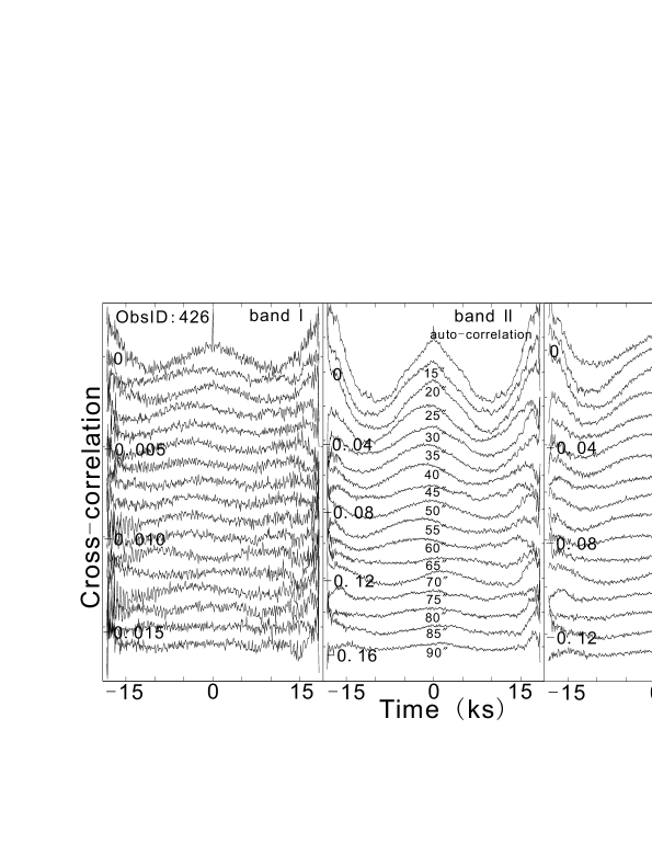
Figure 3: Cross-correlation curves of ObsID426.

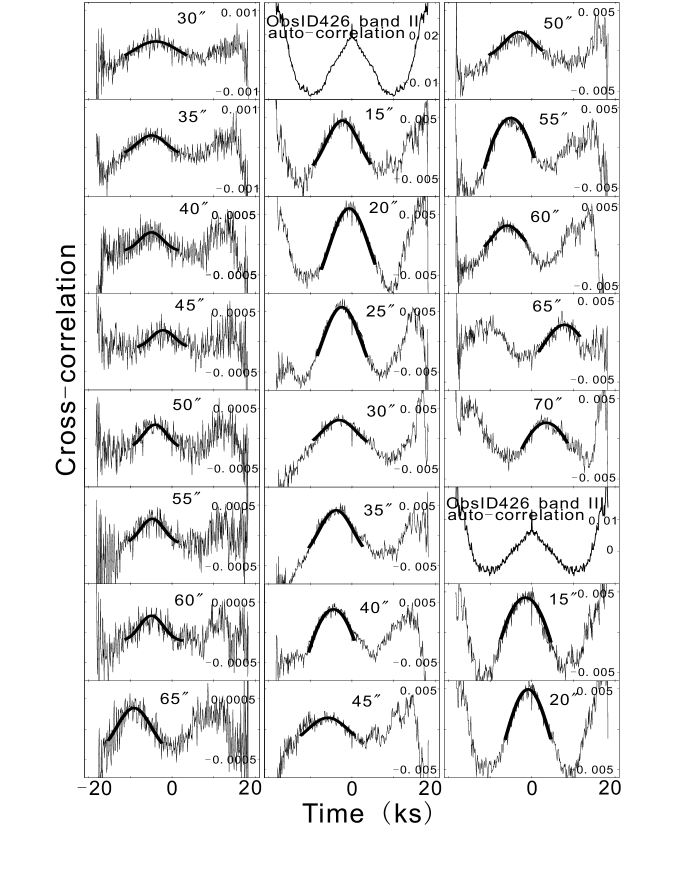
Figure 7: Fig.5 continued.

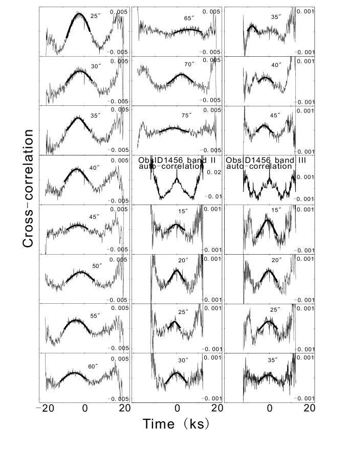
Figure 8: Fig.5 continued.

References

- (1) Avni, Y., 1976, ApJ, 210, 642
- (2) Dickey, J.M., 1983, ApJ, 273, L71
- (3) Hu, J., Zhang, S. N., & Li, T. P. 2004, ApJ, 614, L45
- (4) Humphreys, R. M. 1978, ApJS, 38, 309
- (5) Hutchings, J. B. 1981, PASP, 93, 50
- (6) Kndlseder, J. 2000, A&A, 360, 539
- (7) Kndlseder, J. 2003, in IAU Symp. 212,A Massive Star Odyssey fromMain Sequence to Supernova, ed. K. A. van der Hucht, A. Herrero, & C. Esteban (San Francisco: ASP), 505
- (8) Ling, Z. X., Zhang, S. N., Xiang, J. G., & Tang, S. C. 2009, ApJ, 690, 224
- (9) Matri, J., Paredes, J. M., & Peracaula, M. 2001, A&A, 375, 476
- (10) Massey, P., & Thompson, A. B. 1991, AJ, 101, 1408
- (11) Mathis, J. S., & Lee, C. -W. 1991, ApJ, 376, 490
- (12) Mathis, J. S., Rumpl, W., & Nordsieck, K. H. 1977, ApJ, 217, 425 (MRN)
- (13) Milgrom, M., 1979, A&A, 76, L3
- (14) Overbeck, J. W. 1965, ApJ, 141, 864
- (15) Predehl, P., Burwitz, V., Paerels, F., & Trmper, J. 2000, A&A, 357, L25
- (16) Predehl, P., & Schmitt, J. H. M. M. 1995, A&A, 293, 889
- (17) Rolf, D. P. 1983, Nature, 302, 46
- (18) Smith, R. K., & Dwek, E. 1998, ApJ, 503, 831
- (19) Smith, R. K., Edgar, R. J., & Shafer, R. A. 2002, ApJ, 581, 562
- (20) Thompson, T. W., & Rothschild, R. E. 2009, ApJ, 691, 1744
- (21) TorresDodGen, A. V., Carroll, M., & Tapia, M. 1991, MNRAS, 249, 1
- (22) Trmper, J., & Schnfelder, V. 1973, A&A, 25, 445
- (23) van de Hulst, H.C. 1957, Light Scattering by Small Particle (New York: Dover)
- (24) Vaughan, S., et al. 2004, ApJ, 603, L5
- (25) Vaughan, S., et al. 2006, ApJ, 639, 323
- (26) Weingartner, J. C., & Draine, B. T. 2001, ApJ, 548, 296 (WD01)
- (27) Xiang, J. G., Lee, J. C., & Nowak, M. A. 2007, ApJ, 660, 1309
- (28) Xiang, J. G., Zhang, S. N., & Yao, Y. S. 2005, ApJ, 628, 769
- (29) Yao, Y. S., Zhang, S. N., Zhang, X. & Feng, Y. 2003, ApJ, 59, L43