A noise-driven attractor switching device

Abstract

Problems with artificial neural networks originate from their deterministic nature and inevitable prior learnings, resulting in inadequate adaptability against unpredictable, abrupt environmental change. Here we show that a stochastically excitable threshold unit can be utilized by these systems to partially overcome the environmental change. Using an excitable threshold system, attractors were created that represent quasi-equilibrium states into which a system settles until disrupted by environmental change. Furthermore, noise-driven attractor stabilization and switching were embodied by inhibitory connections. Noise works as a power source to stabilize and switch attractors, and endows the system with hysteresis behavior that resembles that of stereopsis and binocular rivalry in the human visual cortex. A canonical model of the ring network with inhibitory connections composed of class 1 neurons also shows properties that are similar to the simple threshold system.

I introduction

Sensory nerves of several biological systems including cricketscricket , crayfishescrayfish and paddlefishespaddlefish exploit the phenomenon of stochastic resonance (SR) for weak signal detection within a noisy environmentSR . Previous studies concerning cerebral physiology have provided evidence of SR following analysis of hippocampal slices from ratrat_hippocampus and humanhuman_brain1 ; human_brain2 brains. For an adaptive system to successfully operate in an environment, it would be preferable to utilize a certain number of attractors, which represent quasi-equilibrium states into which the system settles until disrupted by environmental change, and an autonomous selection mechanism for one appropriate attractor in the environment. However, the conventional view of SR phenomena lacks the concept that a process switches stochastically to the most preferable attractor. Recently, the concept of neuronal computations with stochastic network states in the brain has also been acceptedneuronal_computation . However, the functional role of noise in neuronal activity remains unknown. In this article, we assembled attractors composed of reverberating electronic circuits in order to investigate the functional role of noise. The results obtained using an SR system based on an excitable threshold systemMP revealed a higher-order function of the SR system and noise-driven attractor switching with a hysteresis phenomenon, which is beyond the well-known functions of noise-driven enhancement on both sensitivity to weak signal detection and signal propagation. In order to examine whether the higher-order function can be extended to more general neuronal models than the simple excitable threshold system, we also performed a numerical simulation for a canonical model of a class 1 neural networkErmentrout ; Ermentrout2 ; Izhikevich1999 ; Izhikevich2 ; Kanamaru1 ; Kanamaru2 ; Kanamaru3 .

II Methods

II.1 A simple excitable threshold unit by an analog electronic circuit

Fig. 1 shows an example of an analog operational amplifier circuit of the simple excitable threshold unit. The circuit is composed of seven functional parts: multiple signal inputs, adder, inverter, comparator, inverter, negative clipper, and an output port. The negative feedback circuits of operational amplifiers with a gain of unity were used for the adder and inverters. We used quad operational amplifiers, TL084 (Texas Instruments, Inc.). The positive and negative electric power source used for the amplifiers was $\pm$ 12 V. The diode for the negative clipper was 1S1558 (Toshiba, Corp., Japan). All the resistors used here are standard metal-film resistors.

II.2 Implementation of an inhibitory connection by an analog electronic circuit

Localization of neuronal excitations is a basic feature of brain function. In order to select an appropriate attractor in a certain environment, inhibitory connections are crucial to the localization of neuronal excitations. It would also be important for the connection to realize attractor switching against environmental change. An inhibitory connection was realized using the variable threshold of the excitable unit. The shutdown of noise generators that is triggered by the output of the other units can also be used as an inhibitory connection. Alternatively, the signal input of the inverted output of the other unit will be available for this purpose.

II.3 Electronic circuit experiments

All data of output voltage for the attractor switching electronic circuit (Figs. 1 and 3) were collected by a multifunction data logger (USB-6008; 12-bit longitudinal digital resolution; maximum sampling rate of 10 kS/sec, National Instruments, Corp.), which was controlled through a general purpose interface bus (GPIB) via a high-speed universal serial bus (USB 2.0). The GPIB and data logger were handled using a graphical user interface built using LabVIEW 8.2 (National Instruments, Corp.). Input signals and threshold voltages were synthesized by standard function generators (WF1974, NF, Corp., Japan). Gaussian white noise was synthesized using a function generator (33120A, Agilent Technologies, Inc.) and fed into the input port of the simple excitable units through an eighth-order Butterworth low-pass filter with a cutoff frequency of 50kHz(two VT-4BLA in box #3334, NF, Corp., Japan). The sampling rate of data collection was 1 k/sec. The average firing rate was determined by averaging digitized output signals during 0.1 s (100 points). The response to the sinusoidal input signal (0.1 V$\times\sin(\omega t)$; $\omega/2\pi$ = 0.3 Hz) was recorded for 18 cycles (only data for the first three cycles is shown in Fig. 3b). The parameters used in Fig. 3b were shown in Table.1.

II.4 Numerical simulation for the network of simple excitable units

The numerical simulation for simple excitable threshold systems was performed using McCulloch-Pitts neuronsMP . Let us consider a ring circuit (Fig. 2c) of $M$ modules(Fig. 2b), where each module is composed of $N$ parallel neurons(Fig. 2a). The output of the $m$-th module with $N$ parallel neurons in ring $X$, $V^{X}_{m}(t)$, at time $t$ is calculated using the following equation:

$$V^{X}_{m}(t) = \frac{1}{N}\sum^{N}_{n=1}{\cal H}[x^{X}_{mn}(t)-V^{\rm Th}_{X}(t)]$$ (6)

$$\left\{\begin{array}[]{l}x^{X}_{\rm 1n}(t)=x^{\rm s}_{1n}(t)+\epsilon^{X}_{\rm M}V^{X}_{\rm M}(t-\tau)+\xi^{X}_{1n}(t)\\ \quad\quad\quad\quad\quad\quad\quad\quad\quad\mbox{if $m=1$}\\ x^{X}_{\rm mn}(t)=\epsilon^{X}_{\rm m-1}V^{X}_{\rm m-1}(t-\tau)+\xi^{X}_{mn}(t)\\ \quad\quad\quad\quad\quad\quad\quad\quad\quad\mbox{if $1<m\leq M$},\end{array}\right.$$

where ${\cal H}[u]$ is a Heaviside step function:

$${\cal H}[u] = \left\{\begin{array}[]{ll}1&\mbox{if $u>0$}\\ 0&\mbox{otherwise}.\end{array}\right.$$ (9)

$V^{\rm Th}_{X}(t)$, $x^{\rm s}_{mn}(t)$, $\xi^{X}_{mn}(t)$ and $\tau$ are the threshold value, sensory signal input, noise for the $n$-th excitable unit in the $m$-th module, and delay time, respectively. For simplicity, all the threshold units in a ring $X$ have the same threshold value($V^{\rm Th}_{X}(t)$). Note that the delay time is important to realize the recurrent network. $\epsilon^{X}_{m}$ is the coupling constant between the $m$-th and $(m+1)$-th modules and is defined as the ratio of the input amplitude of $(m+1)$-module to the output amplitude of the $m$-th module. Noise is represented by the mutually independent and uncorrelated functions

$$\langle\xi^{X}_{mn}(t)\xi^{X}_{pq}(t^{\prime})\rangle = D\delta_{mp}\delta_{nq}\delta(t-t^{\prime})$$ (10)

$$\langle\xi^{X}_{mn}(t)\rangle = 0.$$ (11)

where $\langle\cdot\rangle$ denotes time autocorrelation. The distribution function, $p(x)$, with $\xi^{X}_{mn}(t)=x$ is defined as follows:

$$p(x) = \left\{\begin{array}[]{ll}\mbox{const.}&\mbox{:uniform noise}\\ \frac{1}{\sqrt{\pi D}}\exp(-\frac{x^{2}}{D})&\mbox{:Gaussian noise}\\ \end{array}\right.$$ (14)

The numerical simulations for simple excitable threshold systems were performed on a personal computer with a Core 2 processor (1.86 GHz) and 1 GB of random access memory. A simulation program was written using GNU Octave (version.2.1.73) under the Vine Linux OS (version 3.3.6). All the parameters used in the simulation were dimensionless and summarized in Table. 1.

II.5 Numerical simulation for the ring network with asymmetric inhibitory connections using a canonical model for class 1 neurons

A canonical model of class 1 neurons was employed to further investigate the properties of a two-ring system of stochastically excitable threshold units with inhibitory connections (vide infra). Based on the theory by ErmentroutErmentrout ; Ermentrout2 , IzhikevichIzhikevich1999 ; Izhikevich2 , and KanamaruKanamaru1 ; Kanamaru3 , we interpreted the Langevin equation in the Stratonovich’s sense:

$$\dot{\theta}^{X}_{mn}(t)=(1-\cos\theta^{X}_{mn}(t))+(1+\cos\theta^{X}_{mn}(t))$$

$$\ \ \ \ \times(r_{X}+\xi^{X}_{mn}(t)+K^{{\rm ring},X}_{m}(t)$$

$$\ \ \ \ \ \ \ \ \ +K^{{\rm inh},X}_{m}(t)+K^{{\rm stim},X}_{m}(t)),$$ (15)

where $X=A$ or $B$ and $\theta_{mn}^{X}(t)$, $r_{X}$ and $\xi_{mn}^{X}(t)$ are internal states of the $n$-th neuron in the $m$-th module, the bifurcation parameter for ring $X$, and noise applied for the $n$-th neuron in the $m$-th module, respectively. $\xi_{mn}^{X}(t)$ is uniform white noise with a correlation of

$$\langle\xi_{mn}^{X}(t)\xi_{m^{\prime}n^{\prime}}^{Y}(t^{\prime})\rangle=D\delta_{XY}\delta_{mm^{\prime}}\delta_{nn^{\prime}}\delta(t-t^{\prime}),$$ (16)

where $m,m^{\prime}=1,\cdots,M$ and $n,n^{\prime}=1,\cdots,N$. $\delta_{XY}$, $\delta_{mm^{\prime}}$, and $\delta_{nn^{\prime}}$ are Kronecker delta and $\delta(t-t^{\prime})$ is Dirac’s delta function. $D$ is the noise amplitude. $K_{m}^{{\rm ring},X}(t)$, $K_{m}^{{\rm inh},X}(t)$ and $K_{m}^{{\rm stim},X}(t)$ are signal inputs from the module of the upper stream in the ring, inhibitory signals from ring B to ring A, and the external sinusoidal input, respectively.

$$\left\{\begin{array}[]{l}K_{m}^{{\rm ring},X}(t)=\epsilon_{\rm ex}^{X}I_{m-1}^{X}(t){\rm\ \ \ \ (if\ m\ \neq\ 1)}\\ K_{m=1}^{{\rm ring},X}(t)=\epsilon_{\rm ex}^{X}I_{M}^{X}(t),\\ \end{array}\right.$$ (19)

where $\epsilon_{ex}^{X}$ is the excitatory coupling constant between modules in ring $X$. The asymmetric inhibitory connection is expressed as follows:

$$\left\{\begin{array}[]{l}K_{m}^{{\rm inh},A}(t)=-\ \epsilon_{\rm inh}\sum^{M}_{m^{\prime}=1}I_{m^{\prime}}^{B}(t)\\ K_{m}^{{\rm inh},B}(t)=0,\\ \end{array}\right.$$ (22)

where output current of the $m$-th module, $I_{m}^{X}(t)$, is expressed as an averaging over individual output currents, $I_{mn}^{X}(t)$, of the $n$-th neuron in the $m$-th module of ring X because of the parallel structure of modules (see Fig. 2b),

$$I_{m}^{X}(t) = \frac{1}{N}\sum^{N}_{n=1}I_{mn}^{X}(t)$$ (23)

$$\dot{I_{mn}^{X}(t)} = -\frac{1}{\kappa_{X}}(I_{mn}^{X}(t)-\delta(\theta_{mn}^{X}-\pi)),$$ (24)

and $\epsilon_{\rm inh}$ is the inhibitory coupling constant between rings. A sinusoidal sensory input is applied to the first module ($m=1$) in each ring.

$$K_{m}^{{\rm stim},X}(t)=A_{\rm sig}\sin(\omega t){\rm\ \ \ \ (if\ m=1)},$$ (25)

where $A_{\rm sig}$ and $\omega$ are the amplitude and angular frequency of the sinusoidal input signal, respectively. From Eq.15, 23 and 24, the dynamics of $\theta_{mn}^{X}$ was numerically calculated using an ordinary differential equation solver, ”LSODE”LSODE . All the parameters in the simulation were given in Table. 2.

III Results and Discussion

We focus on a simplified version of a recurrent neural network: a ring circuit. In this architecture, positive feedback is localized to a single ring, which is the minimum component of a complex web of the neural network. We first assembled a memory ring circuit driven by noise. The ring circuit shows a fundamental property of positive feedback that is found in the hierarchy of complex information processing in the human brainAmit ; Iyengar . We explored the properties of a single-ring circuit (Fig. 2c) of $M$ modules (Fig. 2b), where each module was composed of $N$ parallel threshold excitable units (Fig. 2a). This module is the so-called Collins modelCollins with time delay, and it enhances the system’s sensitivity to weak inputs without adjusting the non-zero level of noise amplitude, leading to enhancement of weak signal detection and therefore signal propagation in sensory neurons. The numerical simulation for simple excitable threshold systems was performed using McCulloch-Pitts neuronsMP with uniform white noise, and dimensionless parameters were used to maintain the generality of the problem. The threshold and output amplitudes are defined as $V^{\rm Th}_{m}$ and $V_{m}$, respectively, and the details of the simulation are shown in Sec.II.D and the caption of Fig. 2. We looked at the stochastic response of the ring as a function of the number of parallels ($N$) in each module(Fig. 2d). In Fig. 2d, the pulsed sinusoidal signal is stored in the ring as a form of summed neuronal spikes if independent noise with appropriate amplitude is applied to each unit. An extended lifetime of the stored signal was observed with increasing $N$ (Fig. 2d).

In addition to the structural factor of ring circuits, we found that the noise amplitude and inter-module coupling constant were important in determining the decay rate of transient memory storage. Phase diagrams of the decay rate of memory (Fig. 2e) and signal-to-noise ratio (SNR) of the peak at a frequency of sinusoidal input in the Fourier power spectrum (Fig. 2f) were obtained by numerical simulation (see Sec.II.D) as functions of the inter-module coupling constant ($\epsilon$) and noise amplitude ($D$) for the single ring of $(M,N)$ = (4,100). The rate was determined from the full-width at half-maximum ($\Delta\omega$) of the peak at the dimensionless input frequency ($\omega/2\pi=6.25\times 10^{-2}$) of a fast Fourier power spectrum, and the value of SNR was defined as the ratio of the peak intensity with the averaged noise intensity at 100 points of the proximate baseline over the higher frequency than $\omega+\Delta\omega$. A transient memory domain appears between the non-firing domain (”NF”) and the reverberating domain (”R”) (Fig. 2e). The SNR under conditions of a noise amplitude comparable to the perithreshold signal tends to be largely irrelevant with regard to the coupling constant when $\epsilon>0.05$ (Fig. 2f), and $\epsilon$-slice (slice at the constant $\epsilon(0.05<\epsilon<0.20)$) of Fig. 2f indicates the typical property of stochastic resonance, where application of noise with non-zero amplitude enhances SNR of the spectrumSR . Apparently, variation of the decay rate depended on the noise amplitude, suggesting that noise plays an important role for signal transmission in the ring and that the various energetic states of the reverberating circuit can be defined using the firing rate, leading to the creation and stabilization of attractors (vide infra).

Taking into account the behavior of transient memory storage of the ring, we designed an attractor switching electronic circuit integrated with inhibitory connections (Fig. 3a). Inhibitory connections are important in various neural functions such as binocular rivalry in the visual cortexWilson and dynamical encoding of an olfactory systemLaurent . In particular, the spatio-temporal dynamics of the locust olfactory system are important for the coding of odor intensity and identityStopfer . Our device is composed of two ring circuits with excitable modules. The output of ring B ($\epsilon V^{\rm B}_{m}=0.25$V) is inhibitory and connected to ring A via feeding into the threshold setting port of ring A (Fig. 3a; see also Sections II.A and II.B for details), insuring that either ring A or B can fire. From the electronic circuit experiment and numerical simulation, the behavior of transient memory storage brings about a switching effect in the device (Figs. 3b and 4a–c). The default threshold value of ring A ($V_{\rm A}^{\rm Th}=0.03$V for the experiment and 0.05 for the simulation) was set much lower than that of ring B ($V_{\rm B}^{\rm Th}=0.06$V for the experiment and 0.20 for the simulation), which forces ring A to be more likely to fire than ring B. If the input signal amplitude or mean pulse input rate is large enough to fire ring B, then output A is depressed. Even if the input signal decreases to subthreshold for ring B, ring B reverberates for a while due to its transient nature. But ring A is disinhibited after the rest of ring B. In such a system, we can define a two-dimensional attractor as ($R_{\rm A}$, $R_{\rm B}$) in the phase space, where $R_{\rm A}$ and $R_{\rm B}$ are the firing rates of rings A and B, respectively.

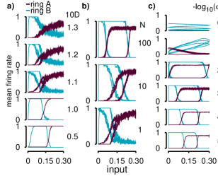
Figure 4: (Color online) (a) The simulated mean firing rate for the devices with ($M,N$) = (4,1). The parameters for the simulation were as follows: $V^{\rm Th}_{\rm{}_{A}}$: 0.05, $V^{\rm Th}_{\rm B}$: 0.20, $\epsilon V^{\rm A}_{m}$: 0.30, and $\epsilon V^{\rm B}_{m}$: 0.30. $D$ was set to 0.05, 0.10, 0.11, 0.12, and 0.13. The other parameters were set to values as indicated in Fig. 2 and also in Table 1 in Appendix. The inhibitory connection was implemented by varying the threshold amplitude: $V^{\rm Th}_{\rm{}_{A}}$ = 0.05 at the disinhibition state and 2.00 at the inhibition state. (b) The response of the device was explored as a function of $N$ while $D$ was fixed at 0.11. (c) The frequency response of the device with $N=100$ and $D=0.11$ is shown. The moderate sweep frequency was necessary for hysteresis behaviors.

The application of noise with an appropriate amplitude endows the electronic circuit with a hysteresis effect (Fig. 3b), and the numerical simulation of the device qualitatively reproduced this experimental tendency (Fig. 4a). Interestingly, noise with an appropriate amplitude (see the curves for $D=2.2$ and $2.4$V in Fig. 3b and for $D=0.11$ and $0.12$ in Fig. 4a) is required for the device to show a clear hysteresis curve. The hysteresis effect is due to the noise-driven transient memory storage effect of ring B and the asymmetric inhibitory connection. During the down-sweeping process of the input signal amplitude, the switching voltage becomes much lower than $V_{\rm B}^{\rm Th}$ because of the above-mentioned reverberation of ring B. During the up-sweeping process, the onset voltage of the firing of ring B can be determined only by $V_{\rm B}^{\rm Th}$ and the noise amplitude, giving a higher switching voltage than that of the down-sweeping process. Thus, the ring network circuit of the excitable threshold system with inhibitory connections allows attractor switching with a hysteresis phenomenon. Additionally, the number of $N$ greatly affected the hysteresis (Fig. 4b). A device with the larger $N$ produced the larger coercivity in the hysteresis loop, indicating that the device would be tied to past memory rather than new environmental sensory input. Furthermore, the device with larger $N$ behaved more deterministically and less probabilistically, and vice versa. From the above discussion, we found the higher-order function that originated from SR; that is, noise-driven signal propagation causes the transient memory effect of the ring, which in turn provides the function of a noise-driven attractor switching effect with hysteresis.

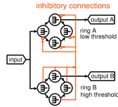
Figure 5: (Color online) A circuit diagram of the attractor switching device. The output signals of all the modules in ring B were fed into the signal input ports of all the modules of ring A.

In order to investigate whether the above-mentioned property of the two-ring system with asymmetric inhibition can be generalized to other neuronal models, we performed the similar simulation using a canonical model of a class 1 neural networkErmentrout ; Izhikevich1999 ; Kanamaru2 . Details of the conditions for the simulation are given in the caption of Fig. 6 and Sec.II.E. Figs. 6a-c show the variation of dependence of mean firing rate for the fourth module ($m=4$) of rings A and B on noise amplitude ($D$), the number of parallels ($N$) in a module, and input frequency ($\omega$), respectively (see Fig. 5 for device architecture). The qualitative tendencies with respect to $D$, $N$ and $\omega$ were the same as those for the simple threshold system described above (Fig. 4); that is, i) noise with proper amplitude is required for the device to show clear hysteresis, and ii) the larger the number of $N$ and input frequency, the larger the coercivity of hysteresis, and iii) the moderate sweep frequency is required to draw clear hysteresis.

The results shown by the simple threshold system and the canonical model of a class 1 neural network are phenomenologically consistent with recent results showing hysteresis effects in stereopsis and binocular rivalry in humansWilson_hysteresis . In the literature, hysteresis is measured as a function of orientation disparity in tilted gratings in which a transition is perceived between stereopsis and binocular rivalry. A fast tilting rate, which corresponds to high-frequency input in our case, results in enhancement of coercivity. Furthermore, a smaller optical Michelson contrast of a sinusoidal grating causes a larger coercivity. A previous functional magnetic resonance imaging study concerning a general mechanism for perceptual decision-making indicated that several brain regions associated with the attentional network show a greater response when the task becomes more difficultdecision_making . Since a test with a smaller grating contrast involves a more difficult task, the region requires more attentional resources for correct performance; that is, the number of neurons (corresponding to $N$) associated with the task could be larger. This is consistent with our result that the device with larger $N$ gives larger coercivity.

The current type of stochastically excitable threshold device in our study essentially requires two parts: a noise generator and comparator. If these components are represented by novel materials beyond silicon materials, novel bio-inspired devices will be realized. Critical dynamics near the phase transition point at ambient temperature will be available to the noise generator if the dynamics are coupled to physical properties such as electric conductivity. Furthermore, field-induced phase transition will be of practical importance in realizing the comparator. Future development on suitable materials for the comparator with a threshold voltage much lower than that of conventional analog operational amplifiers (namely, conventional transistors) will yield attractor switching devices with ultra-low energy consumption like the brain.

IV Conclusion

Problems with artificial neural networks originate from their deterministic nature and inevitable prior learnings, resulting in inadequate adaptability against unpredictable, abrupt environmental change. In this article we showed that a stochastically excitable threshold unit can be utilized by these systems to partially overcome the environmental change; that is, timing of attractor switching is varied depending on not only on the sensory input but also on the memory stored in the ring. Noise-driven attractor stabilization and switching were embodied by a multiple ring network with inhibitory connections. Noise works as a power source to stabilize and switch attractors, and endows the system with hysteresis behavior that resembles that of stereopsis and binocular rivalry in the human visual cortex. In order to further investigate the property of the multiple ring network with inhibitory connections, we performed the numerical simulation of a canonical model of class 1 neurons, where the result showed properties that were similar to the simple threshold system. The device shown in this article will also inspire the material science and engineering in fabrication of noise generators and comparators using functional materials with critical dynamics near the phase transition at ambient temperature and/or field-induced phase transition.

V Acknowledgments

This research was supported by “Special Coordination Funds for Promoting Science and Technology: Yuragi Project” of the Ministry of Education, Culture, Sports, Science and Technology, Japan.

VI Appendix

VI.1 Parameters for numerical simulation and electric circuit experiments

Here we provide all the parameters for the numerical simulations. For the simulation of simple threshold units, the parameters for the simulations in Figs. 2d-f and 4a-c were tabulated in Table1.

For the sumulation of the canonical model of a class 1 neurons(Fig. 6), All the parameters are tabulated in Table 2.

Table 1: Parameters for the numerical simulation of simple threshold units shown in Figs. 2d-f and 4a-c.

	numerical simulations					elec.circuit
figure number	2d	2e and f	4a	4b	4c	3b
$M$	4					4
$N$	1 – 1000	100	1	1 – 100	100	1
$V^{\rm Th}_{m}$	0.10	0.20	-	-	-	-
$\epsilon V_{m}$	0.16	0 – 0.50	-	-	-	-
$t_{\rm pw}$	128		-	-	-	-
$V^{\rm Th}_{A}$	-	-	0.05			0.03V
$V^{\rm Th}_{B}$	-	-	0.20			0.06V
$\epsilon V^{A}_{m}$	-	-	0.30			0.16V
$\epsilon V^{B}_{m}$	-	-	0.30			0.25V
$\omega/2\pi$	6.25$\times 10^{-2}$(=1/16)				10-5 – $10^{0}$	0.3Hz
$D$	0.10	0 – 0.50	0.05 – 0.13	0.11		1.6V – 2.8V
$\tau$	16					-
time-step	1					1$\times 10^{-3}$s
averaging time	64					0.1s

Table 2: Parameters for the numerical simulation shown in Fig. 6.

figure number	6a	6b	6c
$M$	4
$N$	50	1,4,10,25,50	50
$r_{A}$	-0.008
$r_{B}$	-0.020
$\epsilon_{ex}^{A}$	0.5
$\epsilon_{ex}^{B}$	0.5
$\epsilon_{inh}$	3.0
$A_{\rm sig}$	0.019
$\omega/2\pi$	1.0$\times 10^{-3}$		$2.0\times 10^{-4}$ – $5.0\times 10^{-3}$
$D$	6.0$\times$10-4 – 1.4$\times$10-3	1.0$\times$10-3	1.0$\times$$10^{-3}$
$\kappa_{A}$	1.5
$\kappa_{B}$	1.5
time-step	0.05
averaging time	50

Figure 1: Analog electric circuit diagram of a simple excitable threshold unit (McCulloch-Pitts neuronMP ). The unit consists of external signal inputs including sensory signals and signals from the other modules or rings, external noise input, a summation of these components, a successive comparator and an output port. The negative clipper is inserted between the comparator and output port in order to insure that an output with asymmetric voltage is obtained. $R_{1}$ and $R_{2}$ are 10 k$\Omega$ and 100 k$\Omega$, respectively. We used quad operational amplifiers, TL084 (Texas Instruments, inc.). The positive and negative electric power source used for the amplifiers was $\pm$ 12 V.

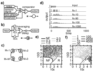
Figure 2: (a) An excitable unit is composed of the following four parts: signal input ports (an external sensory input, the signals from the other units, and external noise), summation of these input signals, a successive comparator, and an output port. The dimensionless output amplitude of the comparator is set to unity. (b) A summing parallel network module (number of units: $N$) of the excitable units of (a), with time delay. This is a version of the so-called Collins-type excitable networkCollins with time delay. The input signal is fed into the input port of each unit. Signal averaging is performed prior to the delay. (c) A ring circuit consists of $M$ directionally coupled modules (b). The value $\epsilon$ denotes the coupling constant between rings, which scales the output voltage of the rings. (d) Variation of transients of the output signal of the ring circuit of $M=4$ as a function of the number of parallels in a module, $N$. The other parameters used for the simulation were as follows and summarized in Table 1 in Appendix: $\epsilon V_{m}$ ($V_{m}$: output amplitude): 0.16, threshold amplitude of comparators ($V^{\rm Th}_{m}$): 0.10, noise amplitude ($D$): 0.10, signal delay at each excitable unit: 16, input signal function: $\cos(2\pi t/16)$, input pulse width($t_{\rm pw}$): 128, and time-step for all simulations: 1. (e,f) Simulated ($\epsilon,D$) phase diagrams for relaxation rate (e) and signal-to-noise ratio (SNR) (f) for the ring with ($M,N$) = (4,100) are shown. $V^{\rm Th}_{m}$ was 0.20. “NF” at the scale bar of (e) stands for “non-firing.” Note that the scale bar of (f) is nonlinear.

Figure 3: (Color online) (a) A circuit diagram of the attractor switching device. A detailed electric circuit design is presented in Sec.II.A. (b) The experimental result of the device with ($M,N$) = (4,1) rings. The firing rates of the fourth module in both rings was monitored as functions of the input signal and noise amplitudes. The parameters for the experiment were as follows: $\epsilon V^{\rm A}_{m}$: 0.16 V, $\epsilon V^{\rm B}_{m}$: 0.25 V, $V^{\rm Th}_{\rm A}$: 0.03 V, and $V^{\rm Th}_{\rm{}_{B}}$: 0.06 V. $D$ was varied from 1.6 V to 2.8 V with a step of 0.2 V. See Sec.II.C for the details of the experiments.

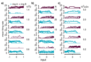
Figure 6: (Color online) The simulated mean firing rate for the canonical model of class 1 neurons as a function of noise amplitude ($D$)(a), the number of $N$(b), and input frequency ($\omega$)(c). $(M,N)$=(4,4), $r_{A}$=-0.008, and $r_{B}$=-0.020. The excitatory coupling constants ($\epsilon_{\rm ex}^{A}$ and $\epsilon_{\rm ex}^{B}$) were 0.5 and the inhibitory connection ($\epsilon_{\rm inh}$) from ring B to ring A was 3.0. For a) and b), the input sinusoidal signal is 0.019$\times$ $\sin(\omega t)$, where $\omega/2\pi$=1.0$\times$10^-3. For b) and c), $D$=1.0$\times$10^-4. For a) and c), $N$=50 The network is composed of slowly connected class 1 neurons with the time constant $\kappa_{A}$=$\kappa_{B}$=1.5. Details of the simulation are given in Sec.II.E and Table 2 in Appendix.

References

- (1) J. E. Levin and J. P. Miller, Nature 380, 165 (1996).
- (2) J. K. Douglas, L. Wilkens, E. Pantazelou, and F. Moss, Nature 365, 337 (1993).
- (3) D. F. Russel, L. A. Wilkens, and F. Moss, Nature 402, 291 (1999).
- (4) L. Gammaitoni, P. Hnggi, P. Jung, and F. Marchesoni, Rev.Mod.Phys. 70, 223 (1998).
- (5) B. J. Gluckman, T. I. Netoff, E. J. Neel, W. L. Ditto, M. L. Spano, and S. J. Schiff, Phys.Rev.Lett. 77, 4098 (1996).
- (6) T. Mori and S. Kai, Phys.Rev.Lett. 88, 218101 (2002).
- (7) K. Kitajo, D. Nozaki, L. M. Ward, and Y. Yamamoto, Phys.Rev.Lett. 90, 218103 (2003).
- (8) A. Destexhe and D. Contreras, Science 314, 85 (2006).
- (9) W. S. McCulloch and W. Pitts, Bull.Math.Biophys. 5, 115 (1943).
- (10) B.Ermentrout, Neural Comput. 8, 979(1996).
- (11) G.B.Ermentrout, Neural Comput. 10, 1047(1998).
- (12) E.M.Izhikevich, IEEE Trans.Neural Networks 10, 499 (1999).
- (13) E.M.Izhikevich, Int.J.Bifurcation and Chaos 10, 1171(2000).
- (14) T.Kanamaru and M.Sekine, Neural Comput. 17, 1315 (2005).
- (15) T.Kanamaru and M.Sekine, Phys.Rev.E 67, 031916(2003).
- (16) T.Kanamaru and M.Sekine, Int.J.Bifurcation and Chaos 16, 3309(2006).
- (17) A.C.Hindmarsh, ACM-SIGNUM Newsletter 15, 10(1980).
- (18) D. J. Amit, Behav.Brain Sci. 18, 617 (1995).
- (19) U. S. Bhalla and R. Iyengar, Science 283, 381 (1999).
- (20) J. J. Collins, C. C. Chow, and T. T. Imhoff, Nature 376, 236 (1995).
- (21) H.R.Wilson, Proc.Natl.Acad.Sci.U.S.A. 100, 14499(2003).
- (22) M.Rabinovich, A.Volkovskii, P.Lecanda, R.Huerta, H.D.I.Abarbanel, and G.Laurent, Phys.Rev.Lett. 87, 068102(2001).
- (23) M.Stopfer, V.Jayaraman, and G.Laurent, Neuron 39, 991 (2003).
- (24) A.Buckthought, J.Kim, H.R.Wilson, Vision Res. 48, 819(2008).
- (25) H. R. Heekeren, S. Marrett, P. A. Bandettini, and L. G. Ungerleider, Nature 431, 859 (2004).