Magnetic Yang-Mills Theory as an Effective Field Theory of the Gluon Plasma

Abstract

We propose magnetic $SU(N)$ pure gauge theory as an effective field theory describing the long distance nonperturbative magnetic response of the deconfined phase of Yang-Mills theory. The magnetic non-Abelian Lagrangian, unlike that of electrodynamics where there is exact electromagnetic duality, is not known explicitly, but here we regard the magnetic $SU(N)$ Yang-Mills Lagrangian as the leading term in the long distance effective gauge theory of the plasma phase. In this treatment, which is applicable for a range of temperatures in the interval $T_{c}\,<\,T\,<\,3\,T_{c}$ accessible in heavy ion experiments, formation of the magnetic energy profile around a spatial Wilson loop in the deconfined phase parallels the formation of an electric flux tube in the confined phase. We use the effective theory to calculate spatial Wilson loops and the magnetic charge density induced in the plasma by the corresponding color electric current loops. These calculations suggest that the deconfined phase of Yang-Mills theory has the properties of a closely-packed fluid of magnetically charged composite objects.

1 Introduction

The confined phase of $SU(N)$ Yang-Mills theory can be described by an effective theory coupling magnetic $SU(N)$ gauge potentials ${\bf C}_{\mu}$ to three adjoint representation Higgs fields [1]. In the confined phase the magnetic gauge symmetry is completely broken via a dual Higgs mechanism in which all particles become massive. The value $\phi_{0}$ of the magnetic Higgs condensate is determined by the location of the minimum in the Higgs potential, and the dual gluon acquires a mass

$$M_{g}\sim g_{m}\phi_{0}\,,$$ (1)

where $g_{m}$ is the magnetic gauge coupling constant. The coupling of the potentials ${\bf C}_{\mu}$ to the magnetically charged Higgs fields generates color magnetic currents which, via a dual Meissner effect, confine $Z_{N}$ electric flux to narrow tubes connecting a quark-antiquark pair [2]. For $SU(3)$, the dual gluon mass $M_{g}\,\sim\,1.95\sqrt{\sigma}$ [3]. The effective theory is applicable at distances greater than the flux tube radius $R_{FT}\sim\frac{1}{M_{g}}\sim 0.3fm$. Since $SU(3)$ lattice simulations [4] yield a deconfinement temperature $T_{c}\,\approx\,0.65\sqrt{\sigma}$, the scale $M_{g}\,\sim\,3T_{c}$. Thus there is a range of temperatures within the interval $T_{c}\,<\,T\,<3\,T_{c}$ where the effective theory should also be applicable in the deconfined phase.

2 Effective Magnetic Yang-Mills Theory of the Deconfined Phase.

Above $T_{c}$ the Higgs condensate vanishes, so the magnetic gluon becomes massless. We assume that the Higgs fields do not play an essential role in the deconfined phase [5]. The effective theory then reduces to pure SU(N) Yang-Mills theory of magnetic gauge potentials ${\bf C}_{\mu}\equiv({\bf C}_{0},{\vec{\bf C}})$. This theory has the same form as the microscopic electric theory, but with a fixed gauge coupling constant $g_{m}\,\sim\,3.91$ and fixed ultraviolet cutoff $M_{g}\,\sim\,3T_{c}\,\sim\,800MeV$, values determined by the effective theory description of the confined phase. The resulting long wavelength magnetic gluons, which at $T=0$ confine $Z_{N}$ electric flux, are the elementary degrees of freedom for $T\,>\,T_{c}$.

We regard magnetic $SU(N)$ gauge theory as an effective field theory appropriate for calculating the long distance magnetic response of the gluon plasma. The dual effective Lagrangian $L_{eff}({\bf C}_{\mu})$ contains all combinations of ${\bf C}_{\mu}$ invariant under magnetic non-Abelian gauge transformations:

$$L_{eff}({\bf C}_{\mu})=2tr\left[-\frac{1}{4}{\bf G^{\mu\nu}G_{\mu\nu}}+\cdots\right]\,,$$ (2)

where

$${\bf G_{\mu\nu}}=\partial_{\mu}{\bf C_{\nu}}-\partial_{\nu}{\bf C_{\mu}}-ig_{m}[{\bf C_{\mu},C_{\nu}}]\,.$$ (3)

Here we retain only the leading term in $L_{eff}$, pure magnetic Yang-Mills theory.

We use effective magnetic Yang-Mills theory to calculate spatial Wilson loops measuring $Z_{N}$ magnetic flux $k$ passing through a loop $L$. These loops are obtained from the partition function of the magnetic theory in the presence of a current of $k$ quarks circulating around the loop $L$, producing a steady current $\frac{2\pi T}{g_{m}}{\bf Y}_{k}$, where ${\bf Y}_{k}$ is a diagonal matrix with the property $e^{2\pi i{\bf Y}_{k}}=e^{2\pi i\frac{k}{N}}$ [6]. This current is the source of an external magnetostatic scalar potential, ${\bf C}_{0}^{ext}=\frac{2\pi T}{g_{m}}{\bf Y}_{k}\frac{\Omega_{S}({\vec{x}})}{4\pi}$, where $\Omega_{S}({\vec{x}})$ is the solid angle subtended at the point ${\vec{x}}$ by a surface $S$ bounded by the loop $L$. Then $\vec{\nabla}{\bf C}_{0}^{ext}=\vec{\bf B}_{BS}$, the Biot-Savart magnetic field of the current loop. (The color magnetic field ${\vec{\bf B}_{j}}={\bf G}_{0j}$.) The spatial Wilson loop of Yang-Mills theory, calculated in the effective magnetic gauge theory, is then the partition function of the magnetic theory in the presence of the external potential ${\bf C}_{0}^{ext}$.

3 The Spatial Wilson Loop Calculated in the Magnetic Theory.

To evaluate the partition function of the magnetic theory in the deconfined phase, where there is no Higgs potential, we must calculate the one loop effective potential $U({\bf C}_{0})$ of magnetic Yang-Mills theory in the background of a static magnetic scalar potential ${\bf C}_{0}$:

$$e^{-\int{d{\vec{x}}\frac{U({\bf C}_{0})}{T}}}\equiv e^{-S^{1-loop}({\bf C}_{0})}=Det\left(-D^{2}_{adj}({\bf C}_{0})\right)\,.$$ (4)

$U({\bf C}_{0})$ is the counterpart in the deconfined phase of the classical Higgs potential generating electric flux tube solutions in the confined phase, and gives rise to the spontaneous breakdown of the $Z_{N}$ symmetry of the effective magnetic gauge theory. We evaluate $U({\bf C}_{0})$ integrating over the massless modes of magnetic Yang-Mills theory, introducing a Pauli-Villars regulator mass $M$. This mass should approximately be equal to the dual gluon mass $M_{g}$ determining the maximum energy of the modes included in the effective theory. Aside from the presence of the regulator, the calculation of $U({\bf C}_{0})$ mimics the calculation [7, 8] of the one loop effective potential $U({\bf A}_{0})$ in Yang-Mills theory used [10, 11] to calculate the spatial ’t Hooft loop [12, 13] . We assume that the background potential ${\bf C}_{0}$ has the same Abelian color structure as ${\bf C}_{0}^{ext}$, i.e., ${\bf C}_{0}=\frac{2\pi T}{g_{m}}C_{0}(\vec{x}){\bf Y}_{k}$. The corresponding dimensionless effective potential $U(C_{0},\frac{T}{M})$ is then a periodic function of $C_{0}$ with period $1$. The resulting expression for the one loop effective action $S^{1-loop}(C_{0})$ is given by [5]

$$S^{1-loop}(C_{0})=\frac{4\pi^{2}\sqrt{3}\,k(N-k)}{N^{3/2}g_{m}^{3}}\int{d{\vec{x}}U(C_{0},\frac{T}{M})}\,,$$ (5)

where

$$U(C_{0},\frac{T}{M})=\left[{[C_{0}]}^{2}(1-[C_{0}])^{2}-\frac{3}{4\pi^{4}}I(C_{0},\frac{T}{M})\right]\,,$$ (6)

and

$$I(C_{0},\frac{T}{M})=\int_{0}^{\infty}{dy\,\,y^{2}log\left(\frac{cosh\sqrt{y^{2}+(\frac{M}{T})^{2}}-cos(2\pi C_{0})}{cosh\sqrt{y^{2}+(\frac{M}{T})^{2}}-1}\right)}\,,$$ (7)

with $[C_{0}]\equiv{|C_{0}|}_{mod1}$. The integral $I(C_{0},\frac{T}{M})$ suppresses the short distance contribution to $U(C_{0})$.

We separate the background scalar potential $C_{0}$ into the contribution $\frac{\Omega_{S}}{4\pi}$ of the external potential and a remaining contribution $c_{0}$ whose sources are the magnetic charges of the plasma:

$$C_{0}=c_{0}+\frac{\Omega_{S}}{4\pi}\,.$$ (8)

Then making the replacement (8) in $S^{1-loop}$ and adding the magnetic energy $(\vec{\nabla}c_{0})^{2}$ of the induced magnetic charges gives the effective action $S_{eff}(c_{0})$:

$$S_{eff}(c_{0})=\frac{4\pi^{2}\sqrt{3}\,k(N-k)}{N^{3/2}g_{m}^{3}}\int{d{\vec{x}}\left[(\vec{\nabla}c_{0})^{2}+{U}(c_{0}+\frac{\Omega_{S}}{4\pi})\right]}\,.$$ (9)

The action (9) generates a mass scale $\frac{Ng_{m}T}{3}$ and a corresponding distance scale which is used in Eqs. (5) and (9). For $T\,>\,T_{c}$ the scale $\frac{Ng_{m}T}{3}$ is greater than the cutoff $M$ so that we can use $S_{eff}$ at the classical level to determine the leading long distance behavior of spatial Wilson loops in the deconfined phase in the same manner that the classical gauge-Higgs action was used to evaluate temporal Wilson loops in the confined phase.

The minimization of $S_{eff}(c_{0})$ yields ”Poisson’s equation” for $c_{0}$:

$$\nabla^{2}c_{0}(\vec{x})=\rho_{mag}(\vec{x})\,,$$ (10)

where

$$\rho_{mag}(\vec{x})=\frac{1}{2}\frac{dU(c_{0}+\frac{\Omega_{S}}{4\pi},\frac{T}{M})}{dc_{0}}$$ (11)

is the color magnetic charge density induced in the vacuum by the current loop. The boundary conditions on $c_{0}$ are: for $\vec{x}$ on $L$, $c_{0}(\vec{x})\rightarrow 0$, and as $\vec{x}\rightarrow\infty$, $c_{0}(\vec{x})\rightarrow-\frac{\Omega_{S}(\vec{x})}{4\pi}$. The latter condition means that the induced magnetic charges screen the external field so that the total field $\vec{B}(\vec{x})=\vec{\nabla}{c_{0}}+\vec{B}_{BS}$ has an exponential falloff determined by the ”Debye” magnetic screening mass $m_{mag}(T)$. In unscaled units

$$m_{mag}^{2}(T)=\frac{N{g_{m}}^{2}T^{2}}{6}\frac{d^{2}U(C_{0},\frac{T}{M})}{dC_{0}^{2}}\bigg{|}_{C_{0}=0}\,.$$ (12)

The value $S_{eff}(L)$ of $S_{eff}(c_{0})$ at its minimum determines the spatial Wilson loop $W(L)=e^{-S_{eff}(L)}$.

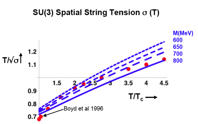
Figure 1: Comparison of $SU(3)$ 4d lattice data (dots) [14] for the spatial string tension $\sigma(T)$ with the prediction of the effective magnetic Yang-Mills theory for four values of the Pauli-Villars regulator mass $M$.

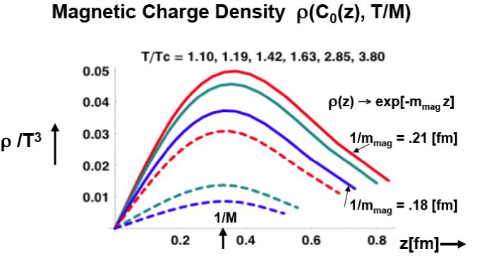
Figure 2: Induced magnetic charge densities $\rho(z)$ outside a large Wilson loop for varying temperatures.

4 Spatial String Tension and Induced Magnetic Charge Density

As $L\rightarrow\infty$ , $S_{eff}(L)\rightarrow L^{2}\sigma_{k}(T)$, determining the spatial string tension $\sigma_{k}(T)$. In this limit the solid angle $\Omega_{S}=-2\pi$ for $z>0$ and $2\pi$ for $z<0$, where $z=0$ is the plane of the loop $L$. The boundary condition at large distances becomes $c_{0}\rightarrow\pm\frac{1}{2}$ as $z\rightarrow\pm\infty$, and $c_{0}$ becomes a function only of $z$. Evaluating $S_{eff}(c_{0})$ at the ”classical” solution $c_{0}(z)$ yields:

$$\frac{\sigma_{k}(T)}{T^{2}}=\frac{8\pi^{2}k(N-k)\int_{0}^{1}dC_{0}\sqrt{U(C_{0},\frac{T}{M})}}{g_{m}{\sqrt{3N}}}\,.$$ (13)

Eq. (13) is valid for any $SU(N)$ group, but the values of $g_{m}$ and $M_{g}$ have been determined only for $SU(3)$ where the effective theory has been applied in the confined phase. The temperature dependence of the ratio $\frac{\sigma_{k}(T)}{T^{2}}$ comes from the Pauli-Villars cutoff, which suppresses the contributions of momenta greater than $M$ to the effective potential (6) and consequently to $\sigma_{k}(T)$. Since the Pauli-Villars regulator is rather ”soft”, allowing substantial contributions from momenta greater than $M$, we have also evaluated the string tension using values of $M$ smaller than $M_{g}\sim 800MeV$. In Fig. 1 we plot $\frac{T}{\sqrt{\sigma(T)}}$, Eq. (13) for $SU(3)$, as a function of $\frac{T}{T_{c}}$ for a range of values of $M$ and compare with the results of 4d lattice simulations [14]. (Values of $M$ lying between $600MeV$ and $650MeV$ give the best fits to the lattice data in the temperature interval $T_{c}\,<\,T\,<\,3\,T_{c}$.)

In Fig. 2 we plot, for a range of temperatures using $M=600MeV$, the magnetic charge density (11) induced by a large Wilson loop as a function of the distance from the loop. For these temperatures the induced distributions $\rho(z)$ of magnetic charge have maxima for values of $z$ close to $\frac{1}{M}\sim 0.33fm$. This can be understood since $\frac{1}{M}$ is the shortest wavelength of the quanta contributing to $U$ and hence determines the spatial extension of the magnetically charged objects described by effective theory. Their ”size” $\frac{1}{M}$ is greater than the magnetic screening length $\frac{1}{m_{mag}(T)}$ determining the exponential tail of the charge distributions as $z\rightarrow\infty$.

In a dilute plasma of charged ions the size of the ion cloud is determined by the Debye screening length which is much larger than the mean separation between the ions. By contrast, in the gluon plasma the mean distance between the extended charges, determined by their intrinsic size $\sim\frac{1}{M}$, is greater than the screening length characterizing the tail of the distribution. This gives a physical picture of the gluon plasma as a dense (closely-packed) liquid of extended magnetically charged objects. Comparison of the plots in Fig. 2 with correlation functions calculated in lattice simulations of Yang-Mills theory [15, 16] could check this picture.

5 Summary

According to our picture, the plasma phase of $SU(N)$ Yang-Mills theory in a temperature range included the interval $T_{c}\,<\,T\,<\,3\,T_{c}$ is described by effective magnetic $SU(N)$ gauge theory. Integrating out the long wavelength non-Abelian degrees of freedom gives rise to extended magnetic charges confining magnetic flux, which are the counterpart in the deconfined phase of magnetic currents confining electric flux in the confined phase. Extension of our work to calculate non-equilibrium quantities would make it possible to use effective magnetic gauge theory to analyze experiments on heavy ion collisions.

References

- [1] M. Baker, J. S. Ball and F. Zachariasen, Phys. Rev. D 44, 3328 (1991).
- [2] S. Mandelstam, Phys. Rep. 23C, 245 (1976); G. ‘t Hooft, , Proceedings of the European Physical Society Conference, Palermo, 1975, ed. A. Zichichi (Bologna, 1976).
- [3] M. Baker, J. S. Ball and F. Zachariasen, Phys. Rev. D 56, 4400 (1997).
- [4] B. Lucini, M. Teper and U. Wenger, Phys. Lett. B 545, 197 (2002) (arXiv:hep-lat/0206029v1).
- [5] M. Baker, Phys. Rev. D 78, 014009 (2008).
- [6] P. Giovannangeli and C. P. Korthals Altes, Nucl. Phys. B608, 203 (2001) (arXiv:hep-ph/0102022v3).
- [7] D. Gross, R. D. Pisarski and L. Yaffe, Rev. Mod. Phys. 53, 43 (1981).
- [8] T. Bhattacharya, A.Gocksch, C. P. Korthals Altes and R. D. Pisarski, Nucl. Phys. B383, 497 (1992); Phys. Rev. Lett. 66, 998 (1991).
- [9] Ph. de Forcrand, B. Lucini and D. North, arXiv:hep-lat/0510081v1.
- [10] C. P. Korthals Altes, A. Kovner and M. Stephanov, Phys. Lett. B346, 94 (1999).
- [11] P. Giovannangeli and C. P. Korthals Altes, Nucl. Phys. B721, 1 (2005) (arXiv:hep-ph/0212298v3); Nucl. Phys. B721, 25 (2005) (arXiv:hep-ph/0412322v2).
- [12] G.’t Hooft Nucl. Phys., B138, 1 (1978); B153, 141 (1979).
- [13] Ph. de Forcrand, M.d’Elia and M. Pepe, Phys. Rev. Lett. 86, 1438 (2001).
- [14] G. Boyd, J. Engels, F. Karsch, E. Laermann, C. Legeland, M. Lütgemeier and B. Petersson, Nucl. Phys. B469, 419 (1996) (arXiv:hep-lat/9602007v1).
- [15] M.N. Chernodub and V.I. Zakharov, Phys. Rev. Lett. 98, 082002 (2007) (arXiv:hep-ph/0611228v2).
- [16] A. D’Alessandro and M. D”Elia, arXiv:hep-lat/0711.1262v2.