A window to quantum gravity phenomena in the emergence of the seeds of cosmic structure

Abstract

Inflationary cosmology has, in the last few years, received a strong dose of support from observations. The fact that the fluctuation spectrum can be extracted from the inflationary scenario through an analysis that involves quantum field theory in curved space-time, and that it coincides with the observational data has lead to a certain complacency in the community, which prevents the critical analysis of the obscure spots in the derivation. We argue here briefly, as we have discussed in more detail elsewhere, that there is something important missing in our understanding of the origin of the seeds of Cosmic Structure, as is evidenced by the fact that in the standard accounts the inhomogeneity and anisotropy of our universe seems to emerge from an exactly homogeneous and isotropic initial state through processes that do not break those symmetries. This article gives a very brief recount of the problems faced by the arguments based on established physics. The conclusion is that we need some new physics to be able to fully address the problem. The article then exposes one avenue that has been used to address the central issue and elaborates on the degree to which, the new approach makes different predictions from the standard analyses. The approach is inspired on Penrose’s proposals that Quantum Gravity might lead to a real, dynamical collapse of the wave function, a process that we argued has the properties needed to extract us from the theoretical impasse described above.

1 Introduction

One of the big problems facing the search for a unification of Quantum Theory and Gravitation is the almost complete absence of experimental data to be used as guidance by theorists. In fact there is up to this date no single man made experiment in which the realms of Quantum Mechanics and Gravitation intersect, i.e. are simultaneously needed to account for the results. The famous COW experiments [1] and the recent “cold neutron” experiments [2] that are some times exhibited as examples of tests of the interface of gravity and quantum mechanics, can not be taken as such when viewed from within the relativistic paradigm, as they can be fully accounted for in terms of physics within a single inertial reference frame, and thus Einsteinian gravity can not be said to be playing any role (for a more detailed discussion of this point see for instance [3]). There exists however one single situation offered to us by nature, which satisfies the two criteria of, being observationally accessible and requiring, for a complete understanding, both general relativity and quantum physics. That is: the origin of the seeds of cosmic structure.

Among the most important achievements in observational cosmology we have the precision measurements of the anisotropies in the CMB[4]. These together with an extensive set of observational studies of large scale matter distribution, led to a very satisfactory picture of the evolution of structure our universe based on a detailed understanding of the physics behind it. In fact it is nowadays widely accepted that the origin of structure in of our universe has its natural explanation within the context of the inflationary scenarios: Inflation takes relatively arbitrary initial conditions presumably emerging from a Planck Era and leads to an almost de-Sitter phase of accelerated expansion that essentially erases all memories of the initial conditions. At this point inflation has lead to a featureless universe, which seems to lack even a small degree of inhomogeneity and anisotropy that is necessary to lead to the subsequent structure formation. At this point quantum mechanics is thought to provide this essential ingredient: The quantum fluctuations of the inflaton field, which has been put by inflation in its “ground state”. These are thought to provide the seeds of the anisotropies and inhomogeneities that eventually evolve into the structure we first see in the CMB and eventually into the obvious features of our universe such as galaxy clusters, galaxies, stars, etc. The remarkable fact is that the calculations based on the above scheme seem to lead naturally to the correct spectrum of these primordial fluctuations.

There is however a serious hole in this seemingly blemish-less picture: The description of our Universe– or the relevant part thereof- starts with an initial condition which is homogeneous and isotropic both in the background space-time and in the quantum state that is supposed to describe the “fluctuations”, and it is quite easy to see that the subsequent evolution through dynamics that do not break these symmetries can only lead to an equally homogeneous and anisotropic universe.

In fact many arguments have been put forward in order to deal with this issue, that is often phrased in terms of the Quantum to Classical transition –without focusing on the required concomitant breakdown of homogeneity and isotropy in the state– the most popular ones associated with the notion of decoherence [16]. These the alternatives have been critically discussed in[5, 6]. One of the main obstacles is that in order to justify any explanation based on decoherence, one has to argue that certain degrees of freedom must be traced over because they are unobservable, and this in turn can only be justified by relying on the limitations we humans currently have, in making certain measurements. The problem is that in so doing we would be using our existence as input, but what cosmology is all about is understanding the evolution of the universe and its structure including the emergence of the conditions that make humans possible. In other words, in order to understand the emergence of an inhabitable universe, we would be relying on the existence and limitations of such inhabitants. Therefore any explanation based purely on standard decoherence becomes circular by definition. There are further problems in each of the specific proposals, and we direct the reader to the above references for extended discussion of this issues. There are other cosmologists that have acknowledged that there is problem here, and that quantum mechanics as we know it needs modifications to be applicable to the cosmology [17], with one of them explicitly stating that decoherence does not offer a complete and satisfactory resolution to this problem [18].

Moreover, if we were to think in terms of first principles, we would start by acknowledging that the correct description of the problem at hand would involve a full theory of quantum gravity coupled to a theory of all the matter quantum fields, and that there, the issue would be whether we start with a quantum state that is homogeneous and isotropic or not?. Even if these notions do not make sense within that level of description, a fair question is whether or not, the inhomogeneities and anisotropies we are interested on, can be traced to aspects of the description that have no contra-part in the approximation we are using. Recall that such description involves the separation of background vs. fluctuations and thus must be viewed only as an approximation, that allows us to separate the nonlinearities in the system–as well as those aspects that are inherent to quantum gravity– from the linear part of problem represented by the fluctuations, which are treated in terms of linear quantum field theory. In this sense, we might be tempted to ignore the problem and view it as something inherent to such approximation. This would be fine, but we should recognize then that we could not argue that we understand the origin of the CMB spectrum, if we view the asymmetries it embodies as arising from some aspect of the theory we do not know, rely on, or touch upon. In fact, in the treatment which we describe next, the proposal is to bring up one particular element or aspect, that we view as part of the quantum gravity realm, to the forefront of the treatment, in order to modify –in a minimalistic way– the semiclassical treatment, that, as we said, we find lacking, and provide a setting in which the obscure issues can at least be focus on. It is of course not at all clear that the problem we are discussing should be related to quantum gravity, but the later is the only sphere which is now believed capable of leading to a radical change in the paradigm of fundamental physics which is of course what we are considering here.

The approach taken in [5] is influenced by Penrose’s suggestion that quantum gravity might play a role in triggering a real dynamical collapse of the wave function of systems [12]. His proposals would have a system collapsing whenever the gravitational interaction energy between two alternative realizations that appear as superposed in a wave function of a system reaches a threshold naturally identified with $M_{Planck}$. We will show that these ideas can, in principle, be investigated in the present context , and that they could lead to observable effects. In fact the very early universe can be seen as a case for which there exists already a wealth of empirical information and one which, as we have argued can not be fully understood without involving some New Physics, with features that would seem to be quite close to those of Penrose’s proposals. There are of course alternatives settings in which modifications of quantum theory, in principle unrelated to Quantum Gravity, could play the role of the New Physics[19] that we have argued is needed in order to account for the seeds of cosmic structure, but we will limit ourselves here to a rather generic setting motivated by the first set of ideas.

2 Quantum Gravity and its effective semiclassical description

Before we present the treatment we are proposing, which should be consider as being of phenomenological nature it is worthwhile to see how would it fit within the context of a fundamental theory such as a quantum theory of gravity.

The first thing one should note is that the notions of space-time are likely to change dramatically when considered in a fully quantum theory of gravitation[7]. A fundamental theory of quantum gravity (with or without matter) is naturally expected to be a timeless theory, but General Relativity is certainly not.

In fact we have a good example of this arising in the past and current attempts to apply the canonical quantization procedure to the theory of General Relativity: In all such schemes one ends with a timeless theory in which the wave functionals $\Psi[h_{ab}]$ depend on (see [10]) a spatial metric $h_{ab}$ associated with a slice $\Sigma$ of space-time (its canonical conjugate momentum $\pi^{ab}$ is a closely related to the extrinsic curvature of such slice $K_{ab}$), or, equivalent variables such as triads and connections as in the modern incarnation of the program known as Loop Quantum Gravity (see for example [11]).

The recovery of the usual space-time notions –that in the appropriate limit should be GR– is thus expected to proceed trough a rather indirect way which involves the identification of one of the variables of the formalism with something playing the role of a physical clock[13], and in fact this seems to be more easily achieved in a theory involving not only the gravitational degrees of freedom, but also some suitable matter fields [14], for instance a scalar field $\phi$, where one would have a wave functional $\Psi[h_{ab},\phi]$. The idea is then that upon the identification of $\phi$ as a physical clock variable, one would be able to talk about the probability that the space-time metric and its conjugate variable take such and such value when the clock takes a given value, and from such information one would presumably be able to estimate the most likely space-time, correlations and so forth. Examples of application of such approach can be seen in [15]. These effective descriptions can be expected quite generally to incorporate some degree of breakdown in unitary evolution [13].

Our point here is that the recovering of the usual space-time picture is expected, to be a complex procedure even if we have a complete theory of quantum gravity in interaction with all matter fields. It should be said that in the LQG program, even the simpler spatial notions as distance volumes and to a lesser degree areas, turn out to be also a rather involved procedure.

The recovery of the standard evolution of physical degrees of freedom in space-time can be expected to involve an even more cumbersome procedure including suitable approximations and averaging. It is thus not unnatural to consider that those might include what we would call “jumps”, and in general the sort of general behavior that would look as an effective collapse of “the wave-function” as seen from the stand point of the effective description. Needless is to say that we have at this time no hope of being able to describe the above procedure in any detail, among other reasons because we do not have at the moment a fully satisfactory and workable theory of quantum gravity.

On the other hand the effective description is expected to lead in the appropriate limit to General Relativity as the description of space-time, and in the corresponding appropriate limit, to quantum field theory for the description of matter fields. We assume that the situation of interest (the inflationary regime of the early universe) lies in a region where both these descriptions are approximately valid, but where some modifications tied to the fact that these picture is only an effective one, need to be incorporated in a seemingly ad hoc manner. Of course we would be complete loss if we did not have any other guidance as to the nature of these modifications, but here is where we look in the opposite direction and guide ourselves on some empirical facts: The inflationary account of the origin of the seeds of cosmic structure works ”almost well” and its defects might be dealt with by the introduction of one such additional feature to the picture. What is required is the assumption of the existence of a process that can take a symmetric (i.e H&I) state of a close system (the Universe), into a state with small departures from a symmetric state while the standard evolution would have preserved those symmetries. As we will see, a quantum mechanical collapse of a wave function seems to have the required characteristics, except that it is usually assumed to be associated with the interaction of the quantum mechanical system with an external classical “apparatus” or “observer”. It is clear that in the situation at hand we can not call upon any such feature so we will assume that the feature in question appears as a self induced collapse, along the lines that have been suggested, based on quite different arguments, as a likely feature of quantum gravity by R. Penrose.

These observations and ideas lead us to consider, situations where a quantum treatment of other fields would be appropriate but an effective classical treatment of gravitation would be justified. That is the realm of semi-classical gravity that we will assume to be valid in our context except at those instants where would break down in association with the jumps or collapses of the state of the quantum field that we considered to be part of the effective description of underlying fundamental quantum theory containing gravitation.

In accordance with the ideas above we will use a semi-classical description of gravitation in interaction with quantum fields as reflected in the semi-classical Einstein’s equation $R_{ab}-(1/2)g_{ab}R=8\pi G\langle T_{ab}\rangle$ whereas the other fields are treated in the standard quantum field theory (in curved space-time) fashion. As indicated this could not hold when a quantum gravity induced collapse of the wave function occurs, at which time, the excitation of the fundamental quantum gravitational degrees of freedom must be taken into account, with the corresponding breakdown of the semi-classical approximation. The possible breakdown of the semi-classical approximation is formally represented by the presence of a term $Q_{ab}$ in the semi-classical Einstein’s equation which is supposed to become nonzero only during the collapse of the quantum mechanical wave function of the matter fields. Thus we write

$$R_{ab}-(1/2)g_{ab}R+Q_{ab}=8\pi G\langle T_{ab}\rangle$$ (1)

Thus, we consider the development of the state of the universe during the time at which the seeds of structure emerge to be initially described by a H.& I. state for the gravitational and matter D.O.F. At some time, $\eta_{c}$, the quantum state of the matter fields reaches a stage whereby the corresponding state for the gravitational D.O.F. is forbidden, and a quantum collapse of the matter field wave function is triggered. This new state of the matter fields does no longer need to share the symmetries of the initial state, and by its connection to the gravitational D.O.F. now accurately described by Einstein’s semi-classical equation leads to a geometry that is no longer homogeneous and isotropic.

That is the approach that is taken in the work presented here, where the intent will be to emphasize the phenomenology potential and the lessons that can be extracted from it in order to make it clear that the proposal can be viewed as a viable path to investigate aspects of the physical world that have for long seemed absolutely beyond reach.

3 The quantum origin of the seeds of cosmic structure

Next we give a short description of the analysis of the origin of the primordial cosmological inhomogeneities and anisotropies based on the ideas outlined above. The staring point is as usual the action of a scalar field coupled to gravity.

$$S=\int d^{4}x\sqrt{-g}[\frac{1}{16\pi G}R[g]-1/2\nabla_{a}\phi\nabla_{b}\phi g^{ab}-V(\phi)],$$ (2)

where $\phi$ stands for the inflaton and for its potential $V$. One then splits both, metric and scalar field into a spatially homogeneous “background” part and an inhomogeneous part “fluctuation”, i.e. the scalar field is written $\phi=\phi_{0}+\delta\phi$, while the perturbed metric can, (after appropriate gauge fixing and by focusing on the scalar perturbation) be written

$$ds^{2}=a(\eta)^{2}\left[-(1+2\Psi)d\eta^{2}+(1-2\Psi)\delta_{ij}dx^{i}dx^{j}\right],$$ (3)

where $\Psi$ is the relevant perturbation called the ”Newtonian potential”.

The background solution corresponds to the standard inflationary cosmology during the inflationary era has a scale factor $a(\eta)=-\frac{1}{H_{\rm I}\eta},$ with $H_{I}^{2}\approx(8\pi/3)GV$while the scalar $\phi_{0}$ field in the slow roll regime so $\dot{\phi}_{0}=-(a^{3}/3\dot{a})V^{\prime}$.

The perturbation of the scalar field leads to a perturbation of the energy momentum tensor, and thus Einstein’s equations at lowest order lead to

$$\nabla^{2}\Psi=4\pi G\dot{\phi}_{0}\delta\dot{\phi}\equiv s\delta\dot{\phi}$$ (4)

where $s=4\pi G\dot{\phi}_{0}$.

We must now write the quantum theory of the rescaled the field $y=a\delta\phi$. For definiteness we consider the field in a box of side $L$, and write the field and momentum operators as

$$\hat{y}(\eta,\vec{x})=\frac{1}{L^{3}}\sum_{\vec{k}}\ e^{i\vec{k}\cdot\vec{x}}\hat{y}_{k}(\eta),\qquad{\hat{\pi}^{(y)}}(\eta,\vec{x})=\frac{1}{L^{3}}\sum_{\vec{k}}\ e^{i\vec{k}\cdot\vec{x}}\hat{\pi}_{k}(\eta),$$ (5)

where the sum is over the wave vectors $\vec{k}$ satisfying $k_{i}=2\pi n_{i}/L$ for $i=1,2,3$ with $n_{i}$ integers, then, we write the fields in terms of the annihilation and creation operators $\hat{y}_{k}(\eta)\equiv y_{k}(\eta)\hat{a}_{k}+\bar{y}_{k}(\eta)\hat{a}^{\dagger}_{-k}$ and $\hat{\pi}_{k}(\eta)\equiv g_{k}(\eta)\hat{a}_{k}+\bar{g}_{k}(\eta)\hat{a}^{\dagger}_{-k}$ with

$$y^{(\pm)}_{k}(\eta)=\frac{1}{\sqrt{2k}}\left(1\pm\frac{i}{\eta k}\right)\exp(\pm ik\eta),\qquad g^{\pm}_{k}(\eta)=\pm i\sqrt{\frac{k}{2}}\exp(\pm ik\eta).$$ (6)

Given that we are interested in considering a kind of self induced collapse which operates in close analogy with a “measurement” which normally involves self adjoint operators, we work find it convenient with the real and imaginary components of the fields and thus we write $\hat{y}_{k}(\eta)=\hat{y}_{k}{}^{R}(\eta)+i\hat{y}_{k}{}^{I}(\eta)$ and $\hat{\pi}_{k}(\eta)=\hat{\pi}_{k}{}^{R}(\eta)+i\hat{\pi}_{k}{}^{I}(\eta)$ where the operators $\hat{y}_{k}^{R,I}(\eta)$ and $\hat{\pi}_{k}^{R,I}(\eta)$ are hermitian. Let $|\Xi\rangle$ be any state in the Fock space of $\hat{y}$,and assign to each such state the following quantity: $d_{k}^{R,I}=\langle\hat{a}_{k}^{R,I}\rangle_{\Xi}.$ The expectation values of the modes of the fundamental field operators are then expressible as

$$\langle{\hat{y}_{k}{}^{R,I}}\rangle_{\Xi}=\sqrt{2}\Re(y_{k}d_{k}^{R,I}),\qquad\langle{{\hat{\pi}^{(y)}}_{k}{}^{R,I}}\rangle_{\Xi}=\sqrt{2}\Re(g_{k}d_{k}^{R,I}).$$ (7)

For the vacuum state $|0\rangle$ we have of course: $\langle{\hat{y}_{k}{}^{R,I}}\rangle_{0}=0,\langle{\hat{\pi}^{(y)}}_{k}{}^{R,I}\rangle_{0}=0,$ while their corresponding uncertainties are

$$(\Delta\hat{y}_{k}{}^{R,I})^{2}_{0}=(1/2)|{y_{k}}|^{2}(\hbar L^{3}),\qquad(\Delta\hat{\pi}_{k}{}^{R,I})^{2}_{0}=(1/2)|{g_{k}}|^{2}(\hbar L^{3}).$$ (8)

The collapse: Next we provide a simple specification of what we mean by “the collapse of the wave function” by stating the form collapsed state in terms of its collapse time. We assume the collapse to be analogous to some sort of imprecise measurement of the operators $\hat{y}_{k}^{R,I}(\eta)$ and $\hat{\pi}_{k}^{R,I}(\eta)$. In order to describe is the state $|\Theta\rangle$ after the collapse we must specify $d^{R,I}_{k}=\langle\Theta|\hat{a}_{k}^{R,I}|\Theta\rangle$. This is done by making the following assumption about the state $|\Theta\rangle$ after collapse:

$$\langle{\hat{y}_{k}^{R,I}(\eta^{c}_{k})}\rangle_{\Theta}=x^{R,I}_{k,1}\sqrt{(\Delta\hat{y}^{R,I}_{k})^{2}_{0}}=x^{R,I}_{k,1}|y_{k}(\eta^{c}_{k})|\sqrt{\hbar L^{3}/2},$$ (9a)

$$\langle{{\hat{\pi}^{(y)}}_{k}{}^{R,I}(\eta^{c}_{k})}\rangle_{\Theta}=x^{R,I}_{k,2}\sqrt{(\Delta\hat{\pi}^{(y)R,I}_{k})^{2}_{0}}=x^{R,I}_{k,2}|g_{k}(\eta^{c}_{k})|\sqrt{\hbar L^{3}/2},$$ (9b)

where $x_{k,1},x_{k,2}$ are selected randomly from within a Gaussian distribution centered at zero with spread one. We note that our universe, corresponds to a single realization of the random variables, and thus each of the quantities $x^{R,I}{}_{k,1,2}$ has a single specific value. Later, we will see how to make relatively specific predictions, despite these features.

The connection to gravitational sector is at the semi-classical level so Eq.(4) turns into

$$\nabla^{2}\Psi=s\langle\delta\dot{\phi}\rangle.$$ (10)

We note that before the collapse, the expectation value on the right hand side is zero. Next we determine what happens after the collapse: To this end, we need to solve the equations (9) for $d_{k}$ and then substitute this in (7) and then in the Fourier transform of Eq.(10) and obtain

$$\Psi_{k}(\eta)=\frac{-s}{k^{2}}\langle\delta\dot{\phi}_{k}\rangle_{\Theta}=\frac{-s}{k^{2}}\sqrt{\hbar L^{3}k}\frac{1}{2a}F(k),$$ (11)

where

$$F(k)=(1/2)[A_{k}(x^{R}_{k,1}+ix^{I}_{k,1})+B_{k}(x^{R}_{k,2}+ix^{I}_{k,2})],$$ (12)

with

$$A_{k}=\frac{\sqrt{1+z_{k}^{2}}}{z_{k}}\sin(\Delta_{k}),\qquad B_{k}=\cos(\Delta_{k})+(1/z_{k})\sin(\Delta_{k}),$$ (13)

and where $\Delta_{k}=k\eta-z_{k}$ with $z_{k}=\eta_{k}^{c}k$.

Turning to the observational quantities we recall that the quantity that is measured is $\frac{\Delta T}{T}$ as a function of $(\theta,\varphi)$, the coordinates on the celestial two-sphere which is expressed as $\sum_{lm}\alpha_{lm}Y_{l,m}(\theta,\varphi)$. The angular variations of the temperature are then identified with the corresponding variations in the “Newtonian Potential” $\Psi$, by the understanding that they are the result of gravitational red-shift in the CMB photon frequency $\nu$ so $\frac{\delta T}{T}=\frac{\delta\nu}{\nu}=\frac{\delta(\sqrt{g_{00}})}{\sqrt{g_{00}}}\approx\Psi$ (we are ignoring, for simplicity the complications of the late time physics such as reheating or acoustic oscillations). Thus, the quantity of interest is the “Newtonian potential” on the surface of last scattering: $\Psi(\eta_{D},\vec{x}_{D})$, from where one extracts $a_{lm}=\int\Psi(\eta_{D},\vec{x}_{D})Y_{lm}^{*}d^{2}\Omega.$ To evaluate the expected value for the quantity of interest we use (11) and (12) to write

$$\Psi(\eta,\vec{x})=\sum_{\vec{k}}\frac{s}{k^{2}}\sqrt{\frac{\hbar k}{L^{3}}}\frac{1}{2a}F(\vec{k})e^{i\vec{k}\cdot\vec{x}},$$ (14)

then, after some algebra we obtain

$$\alpha_{lm} = s\sqrt{\frac{\hbar}{L^{3}}}\frac{1}{2a}\sum_{\vec{k}}\frac{U(k)\sqrt{k}}{k^{2}}F(\vec{k})4\pi i^{l}j_{l}((|\vec{k}|R_{D})Y_{lm}(\hat{k}),$$ (15)

where $\hat{k}$ indicates the direction of the vector $\vec{k}$. It is in this expression that the justification for the use of statistics becomes clear. The quantity we want to evaluate is the result of the combined contributions of an ensemble of collapsing harmonic oscillators each one contributing with a complex number to the sum, leading to what is in effect a bi-dimensional random walk whose total displacement corresponds to the observational quantity. We can not of curse evaluate such total displacement but only its most likely value We do so and then take the continuum limit and which after rescaling the variable of integration to $x=kR_{D}$, becomes

$$|\alpha_{lm}|^{2}_{M.L.}=\frac{s^{2}\hbar}{2\pi a^{2}}\int\frac{C(x/R_{D})}{x^{4}}j^{2}_{l}(x)x^{3}dx,$$ (16)

where

$$C(k)\equiv 1+(2/z_{k}^{2})\sin(\Delta_{k})^{2}+(1/z_{k})\sin(2\Delta_{k}).$$ (17)

In the exponential expansion regime where $\mu$ vanishes and in the limit $z_{k}\to-\infty$ where $C=1$, we find:

$$|\alpha_{lm}|^{2}_{M.L.}=\frac{s^{2}\hbar}{2a^{2}}\frac{1}{l(l+1)}.$$ (18)

which has the standard functional result. However we must consider the effect of the finite value of times of collapse $\eta^{c}_{k}$ codified in the function $C(k)$. We note is that in order to get a reasonable spectrum there is a single simple option: That $z_{k}$ be essentially independent of $k$ that is the time of collapse of the different modes should depend on the mode’s frequency according to $\eta_{k}^{c}=z/k$. There are of course other possible schemes of collapse and we have investigated the most natural ones and their corresponding effects on the primordial fluctuation spectrum, with results that to a large extent confirm that the above conclusion is rather robust (see figure 1, section 5 and specifically [21] for a deeper discussion). Thus we can conclude that the above pattern of times of collapse seems to be implied by the data (as far as our preliminary analysis has shown so far). In our view such conclusion represents one important and relevant piece of information about whatever the mechanism of collapse is.

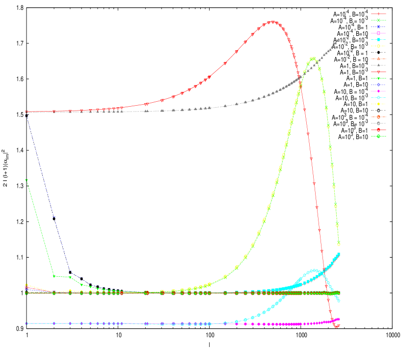
Figure 1: Semi-log plot of $|\alpha_{lm}|^{2}(C_{1}(k))$ assuming a small departure from the result “$z_{k}$ independent of $k$”. This small departure is represented by $\tilde{z}_{x}=A+Bx$, where $x=kR_{D}$, with $R_{D}$ standing for the radius of last scattering surface. Here, we are showing different values of $(A,B)$, representing how robust is the scheme of collapse under this circumstances. The abscissa ranges from $l=0$ to $l=2600$. See section 5 for more details about the meaning of the variables $A$ and $B$.

4 A version of ‘Penrose’s mechanism’ for collapse in the cosmological setting

Based on the analysis of the inadequacies of Quantum Mechanics as a complete theory of nature and the places from where solutions can arise, R. Penrose has argued that the collapse of quantum mechanical wave functions is an actual dynamical process, independent of observation, and that the fundamental physics is related to quantum gravity. More precisely, according to this suggestion, the collapse into one of several coexisting quantum mechanical alternatives would take place when the gravitational interaction energy between the alternatives exceeds a certain threshold. We have considered a naive realization of Penrose’s ideas appropriate for the present setting to be as follows: Each mode would collapse by the action of the gravitational interaction between it’s own possible realizations. In our case, one could estimate the interaction energy $E_{I}(k,\eta)$ by considering two representatives of the possible collapsed states on opposite sides of the Gaussian associated with the vacuum. We interpret $\Psi$, literally as the Newtonian potential and consequently , $\rho=a^{-2}\dot{\phi}_{0}\delta\dot{\phi}$ should be identified with matter density. Then the gravitational interaction energy between alternatives should be:

$$E_{I}(\eta)=\int\Psi^{(1)}\rho^{(2)}dV=(a/L^{3})\dot{\phi}_{0}\Sigma_{k}\Psi^{(1)}_{k}(\eta)\delta\dot{\phi}^{(2)}_{k}(\eta),$$ (19)

where $(1),(2)$ refer to the two different realizations chosen. Recalling that $\Psi_{k}=(-s/k^{2})\delta\dot{\phi}_{k}$, we find

$$E_{I}(\eta)=-4\pi G(a/L^{3})\dot{\phi}_{0}^{2}\Sigma_{k}(1/k^{2})\delta\dot{\phi}^{(1)}_{k}(\eta)\delta\dot{\phi}^{(2)}_{k}(\eta)\approx\Sigma_{k}(\pi\hbar G/ak)(\dot{\phi}_{0})^{2}.$$ (20)

Where we have used equation (8), to estimate $\delta\dot{\phi}^{(1)}_{k}(\eta)\delta\dot{\phi}_{k}^{(2)}(\eta)$ by $|<\delta\dot{\phi}_{k}>|^{2}=\hbar kL^{3}(1/2a)^{2}$.

This result can be interpreted as the sum of the contributions of each mode to the interaction energy of different alternatives. We view each mode’s collapse as occurring independently although at this point it is rather unclear if this can be fully justified, and thus, the collapse of mode $k$ would occur when this energy $E_{I}(k,\eta)=(\pi\hbar G/ak)(\dot{\phi}_{0})^{2}=\frac{\pi\hbar G}{9H_{I}^{2}}(a/k)(V^{\prime})^{2}$ reaches the value of the Planck Mass $M_{p}$. Thus the condition determining the time of collapse $\eta^{c}_{k}$ of the mode $k$ becomes,

$$z_{k}=\eta^{c}_{k}k=\frac{\pi}{9}(\hbar V^{\prime})^{2}(H_{I}M_{p})^{-3}=\frac{\epsilon}{8\sqrt{6\pi}}(\tilde{V})^{1/2}\equiv z^{c},$$ (21)

which is independent of $k$, and thus, as we saw in the previous section leads to a roughly scale invariant spectrum of fluctuations in accordance with observations.

5 Further phenomenological analysis

The scheme of collapse we have considered in section 3, and which will be referred as “the symmetric scheme” or scheme No 1, is evidently far from unique and other similarly natural schemes can be considered here we will briefly discuss two alternatives: “the momentum preferred scheme” or scheme No 2 and the “Wigner functional scheme” or scheme No 3. The first corresponds to the assumption that it is only the momentum conjugate mean value that changes during the collapse according to equation 9 while the field’s expectation value maintains its initial value during the collapse, namely zero. The scheme No 3 corresponds to the assumption that after the collapse the expectation values of field and momentum modes, follow the correlations in the corresponding uncertainties that existed in the of the pre-collapse state, namely:

$$\left\langle\hat{y}_{k}^{(R,I)}\left(\eta_{k}^{c}\right)\right\rangle_{\Omega}=x^{(R,I)}_{k}\Lambda_{k}\cos\Theta_{k}\,,\quad\left\langle\hat{\pi}_{k}^{(R,I)}\left(\eta_{k}^{c}\right)\right\rangle_{\Omega}=x^{(R,I)}_{k}\Lambda_{k}k\sin\Theta_{k},$$ (22)

where $\Lambda_{k}$ is given by the major semi-axis of the ellipse characterizing the bi dimensional Gaussian function (the ellipse corresponds to the boundary of the region in “phase space” where the Wigner function has a magnitude larger than $1/2$ its maximum value), and $\Theta_{k}$ is the angle between that axis and the $y_{k}^{R,I}$ axis.

The subsequent analysis proceeds in the same fashion as that presented in section 3 and the result has the same mathematical expression as in equation (16), with the sole exception being the exact expression of the function $C(k)$, which for the scheme no. 2 takes the form:

$$C_{2}(k)=1+\sin^{2}\Delta_{k}\left(1-\frac{1}{z_{k}^{2}}\right)-\frac{1}{z_{k}}\sin(2\Delta_{k}),$$ (23)

and in the scheme no. 3 is:

$$C_{3}(k)=\frac{32z_{k}^{2}}{\mathcal{A}(1+5z_{k}^{2}-\mathcal{A})}\times\\ \Bigg{\{}\left[\mathcal{A}-1+3z_{k}^{2}\right]\left(\cos\Delta_{k}-\frac{\sin\Delta_{k}}{z_{k}}\right)^{2}+\sin^{2}\Delta_{k}\left[\mathcal{A}-3z_{k}^{2}-7\right]+8z_{k}\cos\Delta_{k}\sin\Delta_{k}\Bigg{\}}.$$ (24)

with $\mathcal{A}=\sqrt{1+10z_{k}^{2}+9z_{k}^{4}}$. In [21] it was shown that, despite the fact that the expression for $C_{3}$ looks by far more complicated that $C_{2}$, their dependence in $z_{k}$ is very similar, except for the amplitude of the oscillations.

These in turn lead to particular forms of the primordial spectrum (i.e the spectrum which emerges from inflation and has not yet been modified to include the late time physics such as the acoustic oscillations responsible for the famous peaks). At the approximation level we are working here the spectra would be all identical to the standard ($n=1$) scale invariant Harrison-Zel’dovich (HZ) spectrum corresponding to a flat line in the graph of $2l(l+1)|\alpha_{lm}|^{2}$ vs. $l$, if we assume that $z_{k}$ is independent of $k$ (corresponding to a time of collapse of mode $k$ given by $\eta_{k}^{c}=z/k$). Therefore, at this level the different collapse schemes are not distinguishable.

We thus were let to considered the sensitivity of the resulting spectrum to small deviations of the “$z_{k}$ independent of $k$ pattern” by studying a linear departure from the $k$ independent $z_{k}$ characterized by $\tilde{z}_{x}$ as $\tilde{z}_{x}=A+Bx$ ($x=kR_{D}$ where $R_{D}$ stands for the radius of the surface of s last scattering) in order to examine the robustness of the various collapse schemes in as far as predicting the observational spectrum.

Some of the results of these analysis can be seen in the graphs 2, 3 in which we see that each collapse scheme leads to a particular pattern of modifications of the spectrum, clearly showing the potential of the present approach to teach us something about the effective collapse, or alternatively to account for possible deviations if anything of this sort were to be detected in future observations.

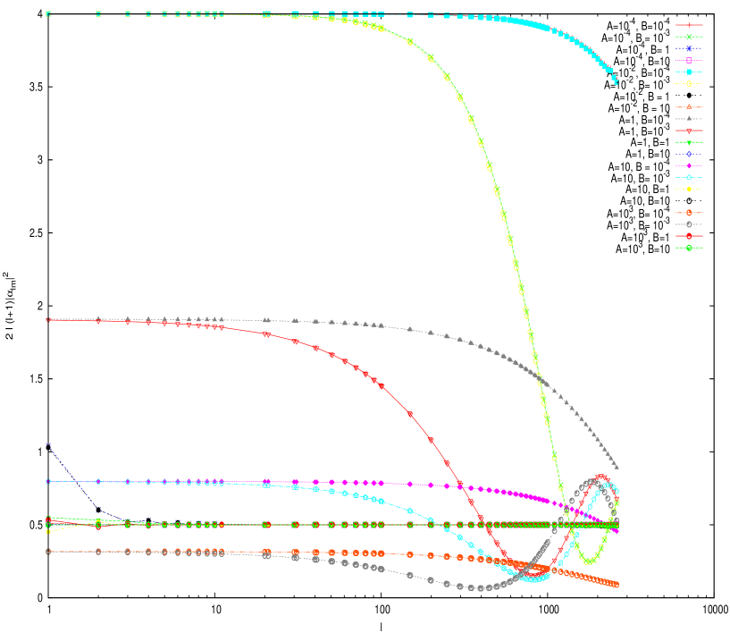
Figure 2: Semi-log plot of $|\alpha_{lm}|^{2}(C_{2}(k))$ for different values of $(A,B)$, representing how robust is the scheme of collapse when it departs from $z_{k}$ constant.The abscissa ranges from $l=0$ to $l=2600$

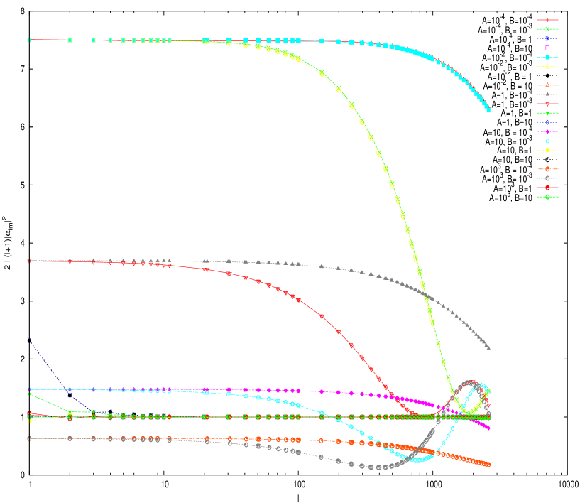
Figure 3: Semi-log plot of $|\alpha_{lm}|^{2}(C_{3}(k))$ for different values of $(A,B)$, representing how robust is the scheme of collapse when it departs from $z_{k}$ constant. The abscissa is $l$ up to $l=2600$.

One of the most important predictions of the scheme, is the absence of tensor modes, or at least their very strong suppression. This can be understood by considering the semi-classical version of Einstein’s equation and its role in describing the manner in which the inhomogeneities and anisotropies in the metric arise in our scheme. As indicated in the introduction, the metric is taken to be an effective description of the gravitational D.O.F., in the classical regime, and not as the fundamental D.O.F. susceptible to be described at the quantum level. It is thus the matter degrees of freedom (which in the present context are represented by the inflaton field) the ones that are described quantum mechanically and which, as a result of an hypothetical fundamental aspect of gravitation at the quantum level, would be subject to an effective quantum collapse (the reader should recall that our point of view is that gravitation at the quantum level will be drastically different from standard quantum theories, and that, in particular, it will not involve universal unitary evolution). This leads to a nontrivial value for $\langle T_{ab}\rangle$, which leads to the appearance of the metric fluctuations. The point is that the energy momentum tensor contains linear and quadratic terms in the expectation values of the quantum matter field fluctuations, which are the source terms determining the geometric perturbations. In the case of the scalar perturbations, there are first order contributions to the perturbed energy momentum tensor, which are proportional to $\dot{\phi}_{0}\langle\delta\dot{\phi}\rangle$, while there are no similar first order terms that would appear as source of the tensor perturbations (i.e. of the gravitational waves). In the usual treatment, and besides its conceptual shortcomings, no such natural suppression of the tensor modes can be envisaged. At the time of the writing of this article, the tensor modes had not been detected, in contrast with the scalar modes.

6 Discussion

We have presented the first steps in the proposal involving the introduction of novel aspect (a self induce collapse of the wave function) of physics in the description of the emergence from the quantum uncertainties in the state of the inflaton field, of the seeds of structure in our universe. We have argued that such novel aspect is likely to be associated to the connection of a fundamental theory of quantum gravity, with the effective description in terms of the equations of semi-classical general relativity. We find it quite remarkable that in doing so, we are able to obtain a relatively satisfactory picture. We do not know what exactly is the physics of collapse but we were nevertheless able to obtain some constraints on it (about the time of collapse of the different modes), and shown that a simplistic extrapolation of Penrose’s ideas satisfy this constraint. We have not investigated the possible connection of our proposal with other more developed schemes involving similar non unitary modifications of quantum theory such as the various schemes considered by colleagues participating in this meeting and others. Te reason for that is that we found it better to try to extract some information about what would be needed for the scheme to work in the cosmological case on which we have centered our interest, and would hope to be able to explore the connections of our proposal, with such schemes an their compatibility of their implications with the conclusions extracted in this initial analysis.

We have reviewed the serious shortcoming of the inflationary account of the origin of cosmic structure, and have given a brief account of the proposals to deal with them which were first reported in [5]. These lines of inquiry have lead to the recognition that something else seems to be needed for the whole picture to work and that it could be pointing towards an actual manifestation quantum gravity. We have shown that not only the issues are susceptible of scientific investigation based on observations, but also that a simple account of what is needed, seems to be provided by the extrapolation of Penrose’s ideas to the cosmological setting. Interestingly the scheme does in fact lead to some deviations from the standard picture where the metric and scalar field perturbations are quantized. For instance, as discussed in the last section, one is lead to expect no excitation of the tensor modes, something that we can expected to be able confront with relatively precise data in the near future.

We also find new avenues to address the fine tuning problem that affects most inflationary models, because one can follow in more detail the objects that give rise to the anisotropies and inhomogeneities, and by having the possibility to consider independently the issues relative to formation of the perturbation, and their evolution through the reheating era (for a more extended discussion of this point see [20]).

Other aspects that can, in principle, be tested, were discussed in the last section. The noteworthy fact is that what initially could have been thought to be essentially a philosophical problem, leads instead to truly physical issues.

Our main point is however that in our search for physical manifestations of new physics tied to quantum aspects of gravitation, we might have been ignoring what could be the most dramatic such occurrence: The cosmic structure of the Universe itself.

It is a pleasure to acknowledge very helpful conversations with J. Garriga, E. Verdaguer and A. Perez. This work was supported in part by DGAPA-UNAM IN108103 grant.

References

References

- [1] Colella R, Overhauser A W and Werner S 1975 Phys. Rev. Let. 34, 1472-1474
- [2] Abele H, Bässler S and Westphal A 2003 in Quantum Gravity From Theory to Experimental Search, ed D Giulini, C Kiefer, and C Lämmerzahl (Berlin: Springer Verlag).
- [3] Chryssomalakos C and Sudarsky D 2003 General Relativity and Gravitation 35, pp 605-617.
- [4] Lange A E et. al. 2001 Phys. Rev. D63, 042001; \nonumHinshaw G et. al. 2003 Astrophys. J. Supp. 148, 135; \nonumGorski K M et. al. 1996 Astrophys. J. 464, L11; \nonumBennett C L et. al. 2003 Astrophys. J. Suppl. 148, 1.
- [5] Perez A, Sahlmann H and Sudarsky D 2006 Class and Quant Gravity 23 2317-54 (Preprint gr-qc/0508100).
- [6] Perez A and Sudarsky A, in preparation Shortcomings in the Understanding of Why Cosmological Perturbations Look Classical .
- [7] Corichi A, Ryan M and Sudarsky D 2002 Modern Physics Letters A 17, 555; \nonumSudarsky D 2008 Int. J. Mod. Physics D17, 425, (Preprint gr-qc/0712.3242).
- [8] Polchinski J 1998 String Theory”, vol. 1: “An introduction to the Bosonic String” and String Theory vol. 2: “Superstring Theory and Beyond” Cambridge University Press, Cambridge.
- [9] Bombelli L, Lee J H, Meyer D and Sorkin R 1987 Phys.Rev.Lett. 59, 521; \nonumSorkin R 2002 in “Valdivia 2002, Lectures on quantum gravity”, pp 305-327, (Preprint gr-qc/0309009).
- [10] Dewitt B S 1967 Phys. Rev. 160, 1113 (1967); \nonumWheeler J A, 1968 in Battelle Rencontres: 1967 Lectures in Mathematics and Physics ed. DeWitt C and Wheeler J A W.A. Benjamin, New York.
- [11] Rovelli C 1998 Living Rev. Rel. 1, 1 (Preprint gr-qc/9710008); \nonumAshtekar A 2001 Quantum geometry and gravity: Recent advance Preprint gr-qc/0112038]; \nonumThiemann T 2001 Introduction to modern canonical quantum general relativity, Preprint gr-qc/0110034.
- [12] Penrose R 1989 The Emperor’s New Mind Oxford University Press; \nonumPenrose R 1996 On Gravity’s Role in Quantum State Reduction Gen. Rel. Grav. 28 pp 581-600 (reprinted in Physics meets philosophy at the Planck scale ed. Callender C. pp 290–304).
- [13] Gambini R and. Pullin J 2004 Phys.Rev.Lett. 93, 240401; \nonumGambini R, Porto R A and Pullin J 2004 Phys.Rev. D70:124001 (Preprint gr-qc/0408050).
- [14] James B. Hartle J B, Hawking S W and Hertog T 2008 Phys.Rev. D77:123537.
- [15] Gambini R, Porto R and Pullin J 2004 New J.Phys. 6 45 (Preprint gr-qc/0402118).
- [16] Halliwell J J 1989 Phys. Rev. D 39, 2912; \nonumKiefer C 2000 Nucl. Phys. Proc. Suppl. 88, 255; \nonumPolarski D and Starobinsky A A 1996 Semiclasicallity and decoherence of Cosmological perturbations Preprint gr-qc/9504030; \nonumZurek W H 1990, Environment Induced Superselection In Cosmology in Moscow 1990, Proceedings, Quantum gravity (QC178:S4:1990), 456-72 (see High Energy Physics Index 30 (1992) No. 624); \nonumLaflamme R and Matacz A 1993 Int. J. Mod. Phys. D 2, 171; \nonumCastagnino M and Lombardi O 2003 Int. J. Theor. Phys. 42, 1281; \nonumLombardo F C and. Lopez Nacir D 2005 Phys. Rev. D 72, 063506; \nonumMartin J 2005 Lect. Notes Phys. 669, 199. \nonumKeifer C, Lohmar I, Polarski D and Starobinsky A A 2006 Preprint astro-ph/0610700.
- [17] Padmanabhan T 1996 Cosmology and Astrophysics Through Problems, Cambridge University Press; \nonumHartle J B 2005 Generalized Quantum mechanics for Quantum Gravity Preprint gr-qc/0510126.
- [18] Mukhanov V 2005 Physical Foundations of Cosmology Cambridge University Press, p 348.
- [19] Ghirardi G C, Rimini A and Weber T 1986 Phys. Rev. D 34, 470 \nonumBassi A 2007 Dynamical Reduction Models: present status and future developments Preprint quant-ph/0701014v2. \nonumBassi A and Ghirardi G C 2003 Dynamical Reduction Models Preprint quant-ph/0302164v2
- [20] Sudarsky D 2007 J. Phys. Conf. Ser. 68, 012029, (Preprint gr-qc/0612005).
- [21] A. De Unanue A and Sudarsky D 2008 Phys. Rev. D 78, 043510 (Preprint gr-qc/0801.4702)