Random Field effects in field-driven quantum critical points

Abstract

We investigate the role of disorder for field-driven quantum phase transitions of metallic antiferromagnets. For systems with sufficiently low symmetry, the combination of a uniform external field and non-magnetic impurities leads effectively to a random magnetic field which strongly modifies the behavior close to the critical point. Using perturbative renormalization group, we investigate in which regime of the phase diagram the disorder affects critical properties. In heavy fermion systems where even weak disorder can lead to strong fluctuations of the local Kondo temperature, the random field effects are especially pronounced. We study possible manifestation of random field effects in experiments and discuss in this light neutron scattering results for the field driven quantum phase transition in CeCu_5.8Au_0.2.

1 Introduction

Disorder effects can strongly modify critical properties close to phase transitions. When investigating the role of disorder, one usually distinguishes two cases: in random-field systems, the disorder couples linearly to the order parameter, while in so-called random mass systems, the coupling is to the square of the order parameter.

Random fields effects are by far more dramatic compared to the random-mass case. As has been shown in a seminal paper by Imry and Ma Imry1 , weak random field even destroys completely long range order for magnets with xy or Heisenberg symmetry as the energy costs to form domain walls are smaller than the energy gain when the magnetic structure adapts locally to the random field. For magnets with Ising symmetry, long range order is stable in three dimensions (3D) as long as the random fields are weak but the properties close to the phase transition are strongly modified.

Random field criticality, and especially the Random Field Ising Model (RFIM), has attracted considerable interests in the last decades. Despite this broad activity reviews including numerical, analytical and experimental investigations, a complete understanding of the RFIM is still lacking. It is established by now that the results of the perturbative RG calculation (the so-called ”dimensional reduction” Aharony1 ; Grinstein ) are incorrect and a consistent theoretical treatment should necessarily rely on some sort of non-perturbative approach. Steps in this direction has been made recently with the help of the functional renormalization group Wiese ; Tarjus1 but the issue of the determination of the correct critical exponents is far from being settled. Moreover, the intrinsic ”glassiness” of the RFIM renders the problem hard to be tackled numerically Middleton1 and, to our knowledge, an unified view of the critical behavior is not yet available. All these complications also arise at a quantum-critical point in the presence of random fields as has been recently discussed by Senthil Senthil .

An important step towards the experimental realization of RFIM was made by Fishman and Ahrony Fishman who suggested to study doped Ising antiferromagnets in uniform magnetic fields. Remarkably, they showed that the net effect of the random moments induced by the non-magnetic doping plus the applied field naturally leads to the same critical behavior as the RFIM. This setup has the unique advantage that one can easily tune the effective strength of the random field just by changing the size of the external uniform field. These observations paved the way for many interesting experiments Belanger1 and for further theoretical work. For example, in a series of recent neutron scattering measures Ye1 ; Ye2 , the lightly-doped iron compound ${\rm Fe_{1-x}Zn_{x}F_{2}}$ showed all the expected features of the RFIM in and out of equilibrium. For this material, an accurate experimental determination of critical exponents was possible.

Recently, also the effects of random-mass disorder close to quantum phase transitions in metallic antiferromagnets have been studied theoretically by a number of authors vojta . Close to the critical point, disorder leads to the formation of magnetic domains. In contrast to the random-mass case these domains are not pinned by external fields and can have stronger fluctuations. This has been predicted to lead to pronounced Griffiths singularities, smeared transitions and glassy states vojta .

In the present paper, we investigate the role of random fields on quantum phase transitions of metallic magnets ignoring the (much smaller) role of random mass effects. As in the setup proposed by Fishman and Ahrony Fishman for classical systems, we consider field driven transition in weakly disordered metallic magnets with Ising symmetry. In these systems, where long range order can exist, the role of the magnetic field is two-fold. On the one hand, coupled to the (non-magnetic) impurities, it generates the random field; on the other hand, it induces a quantum phase transition at a certain critical strength. Field-driven quantum phenomena are today a major topic of experimental investigation, both in the context of magnetic insulators, where the field typically induces a Bose-Einstein condensation of magnons, and in the one of magnetic metals, where the field instead leads to the suppression of the long range order Inga .

Our analysis addresses the latter case. As an example, we have in mind the heavy-fermion compound ${\rm CeCu_{6-x}Au_{x}}$, for which many experimental data are already available in the literature Lohnesyan1 ; Lohnesyan2 . This material is a prototypical heavy-fermion system governed by the competition of Kondo screening and RKKY interactions. For a finite concentration of gold and below a certain critical field, antiferromagnetic Ising order appears at a finite Néel temperature $T_{N}$. For a doping $x>0.1$ the metal orders magnetically at low temperatures. For a doping larger than $0.1$, the magnetic order can be suppressed by a uniform magnetic field which allows a precise study of a field-driven quantum phase transition. The doping by Au atoms naturally induces disorder. For example, a doping $x=0.2$ reduces Lohnesyan1 the effective Kondo temperature on average by approximately 50%. This implies that also the Kondo temperatures will strongly vary locally. Therefore one expects in the presence of a uniform magnetic field rather strong fluctuations in the local magnetization. These static spatial fluctuations play the role of effective random fields and are expected to modify dramatically the properties close to the quantum phase transition. For example, magnetic domains will start to nucleate even on the non-magnetic side of the phase diagram. As we will discuss, recent elastic neutron scattering results from Stockert et al. Stockert appear to be consistent with this scenario.

In this paper, we will not try to describe the critical properties of field driven quantum phase transitions directly at or very close to the quantum critical point. In this regime one has to face all the (unsolved) problems well known from the classical RFIM as has been shown in Ref. Senthil . Instead we will focus on the much more simple, but nevertheless experimentally relevant question, in what regime the quantum-critical properties of the clean system are modified by the random field. What are the signatures of the onset of random-field physics? To answer this question we use standard perturbative renormalization group (RG) methods to determine the properties of the phase diagram and the location of the crossover lines. The perturbative approach is combined with phenomenological considerations based on the Imry-Ma Imry1 argument.

In the following, we first review the derivation of the RG equations Grinstein ; hertz ; Micnas ; Millis and we obtain the general phase diagram with the different physical regimes and crossover lines. Then, we focus on equilibrium and out-of-equilibrium experimental quantities and we list possible smoking guns for the onset of random field physics.

2 Model and perturbative RG equations

The starting point is the usual Landau-Ginzburg-Wilson functional for the order parameter hertz

$$\emph{S}(m) = \frac{1}{2}\sum_{\lambda}\Bigl{[}\Bigl{(}\delta+q^{2}+\frac{|\omega_{n}|}{\Gamma}\Bigr{)}m_{\lambda}m_{-\lambda}+h_{\mathbf{q}}m_{\lambda}\delta_{\omega_{n},0}\Bigr{]}$$ (1)

$$+\frac{u_{0}}{\beta}\sum_{\lambda,\lambda^{\prime},\lambda^{\prime\prime}}m_{\lambda}m_{\lambda^{\prime}}m_{\lambda^{\prime\prime}}m_{-\lambda-\lambda^{\prime}-\lambda^{\prime\prime}}$$

where $m$ is the Ising order parameter, $\lambda=(\omega_{n},\mathbf{q})$, $\Gamma$ is a characteristic energy scale (set to $\Gamma=1$ in the following) and $\delta$ is the critical tuning parameter (proportional to $B-B_{c}$ for a transition driven by a uniform field $B$). The momentum ${\mathbf{q}}={\mathbf{k}}-{\mathbf{Q}}$ is measured with respect to the ordering vector ${\mathbf{Q}}$ of the antiferromagnet and the $|\omega_{n}|$ describes the damping of spin fluctuations by a coupling to particle-hole pairs in a metal. Due to its presence, typical energies scale as $q^{2}$ in the clean system and therefore the dynamical critical exponent is $z=2$. For an insulator (or a metal with small Fermi surface, $2k_{F}<Q$) the $|\omega_{n}|$ is replaced by a $\omega_{n}^{2}$ term such that $z=1$ in this case.

$h(x)$ is the static random field that is assumed to be Gaussian correlated,

$$\langle h(\mathbf{q})\rangle=0\qquad{\rm and}\qquad\langle h(\mathbf{q})h(\mathbf{q}^{\prime})\rangle=h^{2}\delta(\mathbf{q}+\mathbf{q}^{\prime}),$$ (2)

with tunable strength $h$ which is typically proportional to the strength of non-magnetic disorder and, more importantly, to the external uniform field.

With the help of the standard replica trick, we can average over the disorder replicating the action

$$\emph{S}(m^{\alpha}) = \frac{1}{2}\sum_{\lambda,\alpha,\alpha^{\prime}}\Bigl{[}\Bigl{(}\delta+q^{2}+\frac{|\omega_{n}|}{\Gamma}\Bigl{)}\delta_{\alpha,\alpha^{\prime}}-\beta h^{2}\delta_{\omega_{n},0}\Bigr{]}\times$$ (3)

$$\times m_{\lambda}^{\alpha}m_{-\lambda}^{\alpha^{\prime}}+\frac{u_{0}}{\beta}\sum_{\lambda,\lambda^{\prime},\lambda^{\prime\prime}}m_{\lambda}^{\alpha}m_{\lambda^{\prime}}^{\alpha}m_{\lambda^{\prime\prime}}^{\alpha}m_{-\lambda-\lambda^{\prime}-\lambda^{\prime\prime}}^{\alpha}\qquad$$

where $\alpha=1,2..,n$ are the replica-indices. We have formally eliminated the random field and, in absence of the quartic interaction, the free propagator is given by

$$\langle m^{\alpha}_{\lambda}m^{\alpha^{\prime}}_{\lambda^{\prime}}\rangle = \delta_{\lambda,-\lambda^{\prime}}\Bigl{(}\delta+q^{2}+\frac{|\omega_{n}|}{\Gamma}\Bigl{)}^{-1}\Bigl{[}\delta_{\alpha,\alpha^{\prime}}+$$ (4)

$$+ \beta h^{2}\delta_{\omega_{n},0}\Bigl{(}\delta+q^{2}\Bigr{)}^{-1}\Bigr{]}.$$

Observe that already within the Gaussian approximation the propagator at $\omega_{n}=0$ is highly singular in the presence of the random field. Computing the diagrams in Fig. 1 for the replicated action in Eq. (3), we obtain the following closed set of one-loop RG equations (similar to the one obtain by Micnas and Chao Micnas )

$$\frac{d\delta}{d\log b} = 2\delta+6u\emph{f}_{1}(T)+6vf_{2}$$ (5)

$$\frac{dv}{d\log b} = (6-d)v-36uv\emph{f}_{3}(T)-72v^{2}\emph{f}_{4}$$ (6)

$$\frac{du}{d\log b} = [4-(d+z)]u-36u^{2}\emph{f}_{3}(T)-72uv\emph{f}_{4}$$ (7)

$$\frac{dT}{d\log b} = zT(b)$$ (8)

where we defined $v=uh^{2}$ as a renormalized disorder parameter and we introduced the functions $\emph{f}_{n}$ ($n=1,2,3,4$) defined in the appendix. Note that while $f_{1}$ and $f_{3}$ depend both on the renormalized $\delta(b)$ and $T(b)$, the functions $f_{2}$ and $f_{4}$ depend on $\delta(b)$ only as the disorder is static. The upper critical dimension $d=6$ is set by the renormalized disorder $v$. As the classical RG equations Grinstein , Eqns. (5-8) have to leading order in $\epsilon=6-d$ a stable fixed point, $v^{*}=\epsilon/72$, $u^{*}=0$. The critical exponents appear to be given by the ones of the equivalent clean system in dimensions $d^{*}=d-2$ (dimensional reduction, see above).

3 Phase diagram

As already pointed out in the introduction, the pertubative fixed point and the critical exponents are incorrect but they are not our main focus here. We consider instead small bare couplings, $h^{2}\ll 1$ and $u\ll 1$, studying the RG equations in the vicinity of the quantum critical point of the clean system, described by an unstable Gaussian fixed point. Following the flow of the coupling constants, we identify the different crossover lines by investigating for which parameters $\delta$, $v$ or $u$ become of order $1$.

Figure 1: The one-loop diagrams in the presence of disorder. The black dot indicates the random field contribution.

Linearizing Eqns. (5-8) around $u=v=\delta=0$, we obtain

$$\frac{d\delta}{d\log b} = 2\delta+6u\emph{f}_{1}(T)+6v\emph{f}_{2}$$ (9)

$$\frac{du}{d\log b} = [4-(d+z)]u$$ (10)

$$\frac{dv}{d\log b} = (6-d)v$$ (11)

$$\frac{dT}{d\log b} = zT,$$ (12)

where $f_{2}$ is now just a number, and we can write the formal solution

$$\delta(b) = b^{2}\Bigl{[}\delta_{0}+6u_{0}\int_{0}^{\log b}dxe^{[2-(d+z)]x}\emph{f}_{1}(Te^{zx})$$ (13)

$$+6v_{0}\emph{f}_{2}\int_{0}^{\log b}e^{(4-d)x}\Bigr{]}$$

$$u(b) = u_{0}b^{4-(d+z)}$$ (14)

$$v(b) = v_{0}b^{6-d}$$ (15)

$$T(b) = T_{0}b^{z}.$$ (16)

Here $u_{0},v_{0}$ are the bare values of the couplings. Correspondingly, $T_{0}$ is the bare, i.e. the physical temperature. The features of the function $\emph{f}_{1}(T)$ have been already discussed in Millis (see appendix). For our purposes, we only need to know that

$$\emph{f}_{1}(T) \approx \emph{f}_{1}(0)\qquad T\ll 1$$ (17)

$$\emph{f}_{1}(T) \approx CT\qquad T\gg 1$$ (18)

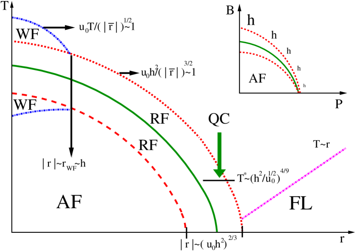
Figure 2: Main figure: Phase diagram for a quantum critical antiferromagnetic metal with Ising symmetry in $d=3$ as a function of temperature and control parameter $r\propto B-B_{c}$ in the presence of random field disorder $h$. Close to the phase transition line, where long-range order vanishes (solid green line), the effects of disorder become dominant (region enclosed by the two dotted red lines parallel to the solid green line). The crossover from the quantum critical to the Fermi liquid regime of the underlying clean system upon lowering $T$ occurs at $T\sim r$ (dotted magenta line). The Wilson Fisher regime of the classical phase transition in the clean limit is only present for $r<-h$ (dotted blue lines at the left part of the diagram). Inset: Phase diagram of a system (e.g. $\rm CeCu_{5.8}Au_{0.2}$) where magnetism can be suppressed either by pressure or an applied magnetic field. As the strength of the effective disorder is proportional to the applied uniform field, $h\propto B$, one can tune the effective strength of random-field disorder.

We first investigate the low-temperature “Fermi liquid” (FL) regime on the disordered side of the phase diagram, see Fig. 2. Here, $\delta(b)$ reaches the cutoff first in a regime where $T(b)\ll 1$ and $v(b)\ll 1$. Using Eq. (17) and expanding Eq. (13), we obtain for $d+z>4$ (we are mainly interested in the metallic, three-dimensional case, $d=3,z=2$)

$$1 = b^{2}[\delta_{0}+\frac{6u_{0}\emph{f}_{1}(0)}{d+z-2}+6v_{0}\emph{f}_{2}\frac{(b^{(4-d)}-1)}{4-d}]$$ (19)

$$\approx b^{2}[\delta_{0}+\frac{6u_{0}\emph{f}_{1}(0)}{d+z-2}]=b^{2}r$$

$$T = T_{0}b^{z}=T_{0}/r^{z/2}\ll 1$$ (20)

$$v = v_{0}r^{(d-6)/2}\ll 1$$ (21)

where $r$ describes the distance from the quantum-critical point of the underlying clean system,

$$r=\delta_{0}-\delta_{0}^{c}=\delta_{0}+\frac{6u_{0}\emph{f}_{1}(0)}{d+z-2}.$$ (22)

The first inequality (20) describes the crossover to the quantum critical regime, see Fig. 2, while the second (21) the onset of a regime, where the random field dominates the critical behavior (see discussion below).

A similar condition for the onset of random-field criticality can be obtained in the ordered phase. Here we use the phenomenological Imry-Ma argument Imry1 . The random field favors the proliferation of magnetic domain walls where each domain (of radius $L$) adjusts itself to the underlying random-field landscape. Far enough from the transition, the energy cost of a domain wall Chaikin is proportional to $\frac{|r|^{3/2}}{u}L^{d-1}$ for $L$ large compared to the correlation length $\xi$. The energy gain from the random field scales with $hmL^{d/2}$ where the size of the order parameter is given by $m=(|r|/u_{0})^{1/2}$. In $d>2$, the size of a random-field induced domain is therefore limited by

$$h\Bigl{(}\frac{|r|}{u}\Bigr{)}^{1/2}L^{d/2}>\frac{|r|^{3/2}}{u}L^{d-1}.$$ (23)

This inequality has an solution with $L>\xi\approx r^{-1/2}$ only for

$$|r|\lesssim(uh^{2})^{\frac{2}{6-d}}.$$ (24)

which is equivalent to the condition (21) obtained from perturbative RG for the disordered side of the phase diagram. Therefore if $|r|$ is sufficiently small, magnetic domains caused by the random field will proliferate while deep in the ordered phase only exponentially rare random-field configurations induce (small) domains.

In $d=2$, the long range magnetic order is always destroyed and fragments into domains. In this case, (24) describes the condition for a crossover from exponentially large domains for large negative $r$ to a disorder dominated regime for smaller $r$ binder .

The quantum critical (QC) regime is obtained when approaching the quantum phase transition by lowering the temperature. In this regime, the rescaled $T(b)=T_{0}b^{z}$ reaches the cutoff, $T(b=b^{*})=1$ where the RG flow changes its nature (but is not stopped). Therefore it is useful to split the RG flow in two steps, rewriting Eq. (13) as follows

$$\delta(b) = b^{2}\Bigl{[}\delta_{0}+6u_{0}\int_{0}^{\log b^{*}(T)}dxe^{[2-(d+z)]x}\emph{f}_{1}(Te^{zx})$$ (25)

$$+6u_{0}\int_{\log b^{*}(T)}^{\log b}dxe^{[2-(d+z)]x}\emph{f}_{1}(Te^{zx})$$

$$+6v_{0}\emph{f}_{2}\int_{0}^{\log b}e^{(4-d)x}\Bigr{]}$$

where we defined $b^{*}(T_{0})=T_{0}^{-1/z}$. Using Eqns. (17) and (18), we can perform the integrals in Eq. (25), to obtain

$$\delta(b) = b^{2}\Bigl{[}r+6u_{0}\bigl{(}\frac{\emph{f}_{1}(0)}{2-(d+z)}+\frac{C}{d-2}\bigr{)}T^{\frac{d+z-2}{z}}$$ (26)

$$+\frac{6v_{0}\emph{f}_{2}}{4-d}b^{4-d}\Bigr{]}.$$

The combination

$$\bar{r}=r+6u_{0}\bigl{(}\frac{\emph{f}_{1}(0)}{2-(d+z)}+\frac{C}{d-2}\bigr{)}T^{\frac{d+z-2}{z}},$$ (27)

can be identified with the distance from the finite-temperature phase transition line Millis .

To find the crossover lines to the random-field dominated regime, we have to investigate under which condition, the term proportional to $v_{0}$ dominates in (26) of the clean system. For $v_{0}=0$, $\delta(b)$ reaches $1$ for $\bar{b}=\bar{r}^{-1/2}$. As the RG flow stops for $\delta(b)>1$, we can obtain the crossover line from the condition $\bar{r}\approx\frac{6v_{0}\emph{f}_{2}}{4-d}{\bar{b}}^{4-d}$. Random field physics therefore dominates for

$$\bar{r}\lesssim(u_{0}h^{2})^{\frac{2}{6-d}}.$$ (28)

This is also the condition that $v(\bar{b})$ becomes of order $1$ (note that $\bar{b}$ and not $b^{*}$ enters here). This last equation is de facto a Ginzburg criterion for the on-set of the random field effects. Notice that Eq. (28) is the extension to finite temperature of Eq. (24) that followed directly from the Imry-Ma argument.

For $r=0$, i.e. in the quantum-critical region of the underlying clean system, the effects of random fields are weak for $T_{0}>T^{*}$ with

$$T^{*} \approx u^{\frac{z(d-4)}{(6-d)(d+z-2)}}h^{\frac{4z}{(6-d)(d+z-2)}}$$ (29)

$$\approx \Bigl{(}\frac{h^{2}}{u^{1/2}}\Bigr{)}^{4/9}\qquad{\rm for}\quad d=3,z=2.$$

according to Eq. (28).

The calculations given above are obviously not valid very close to the classical phase transition of the clean system where also $u$ is relevant. Very close to the QCP this Wilson-Fisher critical regime is never reached because the random field becomes relevant first. Comparing the Ginzburg criterium for the clean system

$$\frac{uoT_{0}}{\bar{r}^{(4-d)/2}}\approx 1.$$ (30)

with Eq. (28), we find that the system will enter the Wilson-Fisher regime of the clean system before the random fields becomes relevant only for $|r|>r_{WF}$ (see Fig. 2) with

$$r_{WF} \approx h^{\frac{8-2d}{6-d}\,\frac{d}{z}}u_{0}^{\frac{6z-dz-2d}{(6-d)z}}$$ (31)

$$= h\qquad{\rm for}\quad d=3,z=2$$

Combining the results for the various crossover lines, we obtain the phase diagram shown in Fig. 2.

4 Experimental probes

As pointed out in the introduction, field driven quantum phase transitions offer a high degree of tunability. An external magnetic field changes not only the distance to the quantum-critical point but also the effective strength of the random-field disorder, $h\propto B$. Ideally, one can use a combination of doping and magnetic field or, even better, of pressure and magnetic field to tune the random field strength and the distance from the QCP independently. For example, considering a system like CeCu_5.8Au_0.2, the quantum critical point can be reached either by applying moderate magnetic fields or a moderate pressure. By crossing the phase transition line in the $B,p$ plane for different values of the magnetic field (see inset of Fig. 2), one can systematically study how random fields modify the physics.

4.1 Elastic neutron scattering and comparison to CeCu_5.8Au_0.2

Elastic neutron scattering probes the static magnetization of the sample as a function of momentum. In a random field system there is always a finite, spatially-fluctuating static magnetization even far away from the transition. In contrast, in a clean system (or in the presence of only random-mass disorder), a finite-momentum static magnetization appears only in the ordered phase footnote .

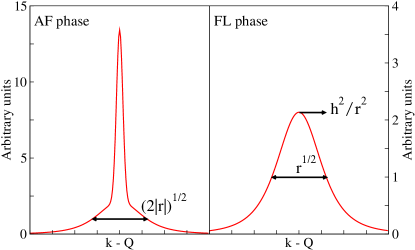
Figure 3: Sketch of the elastic neutron scattering signal in the ordered and disordered phases. Deep in the ordered phase, one expects a resolution limited peak of Gaussian shape at the ordering wave vector. Random fields induce a double-Lorenzian tail of width $\sqrt{2|r|}$, see Eq. (32). Upon approaching the random-field regime, the weight of the tail becomes of the order of the weight of the central peak. Also in the Fermi liquid regime, the random field gives a contribution to the neutron scattering signal described by Eq. (33).

Outside of the random-field regime, i.e for $|r|>(u_{0}h^{2})^{2/3}$ (assuming $d=3$ in this chapter) one can easily estimate the effects of the random field. Even deep in the antiferromagnetic phase, the random fields will induce an extra contribution to the magnetization, $\delta m_{q}\approx\chi_{q}h_{q}$, where $\chi_{q}\approx 1/(-2r+q^{2})$ is the susceptibility of the clean system in the ordered phase ($r<0$) and $q$ measures the distance from the ordering wave vector. Averaging over disorder, we obtain a corresponding contribution to elastic neutron scattering. The total elastic cross section

$$\sigma_{el}(q)\approx m_{0}^{2}\,\,\delta^{3}(q)+\frac{h^{2}}{(|2r|+q^{2})^{2}}$$ (32)

therefore obtains a contribution both from the long-range order and from the random fields. There is also an extra contribution (not shown above) from exponentially rare field-induced domains and the corresponding domain walls. These domains proliferate upon approaching the random-field regime. A schematic picture of the expected neutron signal (including resolution effects) is shown in Fig. 3.

Similarly, approaching the transition from the disordered side one obtains

$$\sigma_{el}(q)\approx\frac{h^{2}}{(r+q^{2})^{2}}$$ (33)

As above, there are some rare regions where the random fields are strong and for which (33) cannot be used but these give only sub-leading contributions for $r>(u_{0}h^{2})^{2/3}$.

For an experiment with finite resolution, it is not possible to separate the two contributions in (32) very close to the transition. In the random-field regime, the weight of the order parameter is always smaller than the weight of the disorder contribution. As a consequence, the phase transition appears to be ’smeared out’.

Qualitatively, such a behavior has been observed in recent neutron scattering experiments on the field-driven QPT in CeCu_5.8Au_0.2 by Stockert et al. Stockert . Upon approaching the transition, the elastic neutron scattering signal broadens and the weight of the signal is reduced. However, there are no sharp features and the integrated intensity remains finite well beyond the critical field. According to Eq. (33), the width of the signal should grow as $\sqrt{r}\sim\sqrt{B-B_{c}}$ while the total integrated intensity vanishes slowly with $h^{2}/\sqrt{r}$ (note that in Ref. Stockert the intensity was obtained by integrating over a rocking scan, i.e. a line in momentum space, leading to a more rapid decay $\sim h^{2}/r^{3/2}$). While the experimental results appear to be consistent with the predicted scenario, a fully quantitative comparison is not possible due to the limited statistics and momentum resolution of the experiment. For a quantitative comparison it would be useful to consider samples with different doping and different critical fields. Ideally, one would like to use both pressure and field to explore the phase diagram sketched in the inset of Fig. 2 using a single sample with fixed bare disorder strength. In such a case, the random field $h$ will be roughly proportional to the critical field $B_{c}$.

4.2 NMR

As a local probe, nuclear magnetic resonance (NMR) is a natural tool to investigate systems with magnetic textures and inhomogeneities. It is possible to measure directly the distribution of the local magnetization $M({\mathbf{r}})=M_{0}+\delta M$. Assuming a Gaussian distribution of the random fields, $p[h(r)]\sim\exp\!\!\left(-\int h(r)^{2}/(2h^{2})\right)$ as in Eq. (2), we can derive the corresponding distribution of magnetic moments outside of the random field regime using again $\delta m_{q}\approx\chi_{\mathbf{q}}h_{q}$ to obtain

$$P(\delta M) \approx \exp\!\!\left(-(\delta M)^{2}/(2\sigma^{2})\right)$$ (34)

$$\sigma^{2} = h^{2}\int\chi_{\mathbf{q}}^{2}\sim\frac{h^{2}}{r^{(4-d)/2}}$$ (35)

For a field-driven quantum phase transition in $d=3$, we therefore expect a width $\sigma$ proportional to $B/(B-B_{c})^{1/4}$.

4.3 Non-equilibrium effects

Probably the most direct way to detect random-field physics, is the observation of hysteretic behavior in the random-field regime which shares similarity to the properties of (spin-) glasses. This is well known both theoretically and experimentally for classical random-field systems. Upon approaching the classical critical point, the relevant relaxation rates grow exponentially Villain ; Fisher ; Nattermann with the correlation length,

$$\tau\sim\exp[c\,\xi^{\theta}/T],$$ (36)

where $\theta$ parameterizes the typical free energy of the system at the scale $\xi$, $F_{\xi}\sim\xi^{\theta}$. For conventional critical points one has $F_{\xi}\sim T\sim const.$. A divergence of $F_{\xi}$ leads to a violation of hyper-scaling, $(d-\theta)\nu=2-\alpha$ ($\nu$ and $\alpha$ are the correlation length and specific heat exponents). Therefore $\theta$ describes to what extent there is an effective dimensional reduction, $d\to d-\theta$. In Ref. Middleton1 , $\theta\approx 1.49\pm 0.03$ was estimated numerically for $d=3$.

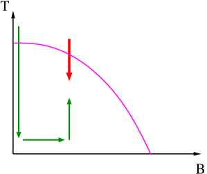
Figure 4: The two non-equivalent cooling procedures. The zero-field cooling path is indicated with the thin green arrows while the field cooling scheme uses a path along the thick red arrow.

Experimentally, the long relaxation rates lead to strong non-equilibrium effects. Neutron scattering experiments Ye2 ; Belanger1 and magnetization measurements Kleemann on diluted antiferromagnets in uniform magnetic fields show hysteretic behavior. It is, for example, useful to compare field-cooled with zero-field cooled samples. Zero field cooling (green arrows in Fig. 4) leads to a well-ordered antiferromagnetic state. Instead, field cooling causes a fragmentation of the antiferromagnet into non-equilibrated domains. The size of the domains depend on the strength of the random field Villain and logarithmically on the cooling rate, see Eq. (36). For example, experiments in field-cooled and zero-field-cooled $\rm Fe_{0.85}Zn_{0.15}F_{2}$, give distinct critical behavior Ye2 ; Belanger1 . Moreover, sweeping fast in temperature back and forth through the transition, can cause the onset of hysteresis phenomena in the intensity of the Bragg peak.

From energetic and renormalization group arguments, it is believed reviews ; Senthil that the static properties of the $T=0$ and finite-temperature random-field transitions are described by the same fixed point. The dynamics and therefore the non-equilibrium properties can, however, differ. For $T\to 0$, the dynamics is not any more governed by thermal fluctuations and thermal activation but instead by quantum tunneling. Nevertheless, the existence of extensive energy barriers, $E_{\xi}\sim\xi^{\theta}$, will lead again Senthil to exponentially long relaxation times

$$\tau\sim\exp[c^{\prime}\,\xi^{\Psi}],$$ (37)

with $\Psi\neq\theta$ for insulators. In a metal, one has furthermore to take into account, that quantum-tunneling can be suppressed Millis1 ; vojta by the coupling of the order parameter to the electrons. This will lead to an additional suppression of the tunneling rate proportional to $T^{c^{\prime\prime}\xi^{\gamma}}$

$$\tau\sim T^{-c^{\prime\prime}\xi^{\gamma}}\exp[c^{\prime}\,\xi^{\Psi}],$$ (38)

with a new (and unknown) exponent $\gamma$ such that $\tau(T=0)=\infty$ for sufficiently large domains.

Note that long relaxation times, smeared transitions and glassy effects can also arise in the absence of magnetic fields, i.e. in systems with random-mass disorder vojta . In general, these effects are expected to be much weaker (the bare scaling dimension of the random-mass disorder is $4-d$ rather than $6-d$). Furthermore, the (bare) strength of the random-mass disorder does not depend strongly on the strength of the external magentic field which allows to separate the two effects.

5 Conclusions

Field-driven quantum phase transitions of antiferromagnets offer a unique possibility to study the interplay of disorder and quantum criticality. Here one has to distinguish two cases: when the staggered magnetization is perpendicular to the applied field (the typical situation for a system with Heisenberg symmetry) and the opposite situation (for Ising symmetry). In the first case, disorder effects are usually weak, the disorder couples only to the square of the order parameter. This paper focuses on the second case, where effectively a random field is generated Aharony1 which couples linearly to the order parameter. In easy plane antiferromagnets, one can have both situations depending on the direction of the magnetic field.

As magnetic domains can nucleate and pin at random field configurations, the critical behavior of the system is radically changed by the presence of disorder. By comparing quantum critical points of the same material at different pressure, different doping or different field direction, one can directly observe how random-fields of different strengths affect quantum criticality.

With the help of perturbative renormalization group we have derived the generic features of the phase diagram for metallic Ising antiferromagnets in weak random fields. While this method is not able to investigate the regime, where random-field physics dominates, one can nevertheless extract the relevant crossover scales. This is especially of interest for the study of systems where the effective strength of random-field disorder can be tuned as described above and in the inset of Fig. 2.

One effect of random fields is that the phase transition appears to be “smeared”. We argue that this has been observed in recent elastic neutron scattering experiments in CeCu_5.8Au_0.2 where the elastic neutron scattering peak broadens and slowly diminishes in weight when the magnetic field is increased beyond the critical field.

The most direct way to detect random-field physics is the observation of hysteretic behavior as a function of temperature and, especially, field. In metals, these non-equilibrium effects are enhanced compared to their classical counterparts as quantum tunneling is inhibited by the coupling to the particle-hole pairs of the metal and thermal activation is suppressed by the low temperatures.

We hope that the high tunability of the random-field physics will motivate further theoretical and especially experimental studies of this very interesting problem.

Appendix A: $f_{n}$ functions

Referring to the case of an itinerant antiferromagnet, in accordance with Millis , the $f_{1}$ function is defined as

$$f_{1} = \frac{\Lambda^{d+z+2}\Omega^{d}}{\pi}\int_{0}^{\Gamma\Lambda^{z-2}}d\omega\coth\frac{\omega}{2T}\frac{\omega}{\Lambda^{2z}(\delta+\Lambda^{2})^{2}+\Lambda^{4}\omega^{2}}$$ (39)

$$+ \frac{2\Gamma^{2}}{\pi}\int_{0}^{\Gamma}\frac{d^{d}q}{(2\pi)^{d}}\coth\frac{\Gamma}{2T}\frac{q^{2+z}}{q^{4}\Gamma^{2}+q^{2z}(q^{2}+\delta)^{2}}$$

where $\Lambda$ is the momentum cut-off, $\Gamma$ is the frequency cut-off, $\Omega_{d}$ is the volume of the surface of unitary radius in $d$ dimensions and $z=2$ is the dynamical exponent. The other functions are instead given by Micnas :

$$f_{2} = \frac{\Omega^{d}\Lambda^{d}}{(2\pi)^{d}}\frac{1}{(\delta+\Lambda^{2})^{2}}$$ (40)

$$f_{3} = -\frac{\partial f_{1}}{\partial\delta}$$ (41)

$$f_{4} = \frac{\Omega^{d}\Lambda^{d}}{(2\pi)^{d}}\frac{1}{(\delta+\Lambda^{2})^{4}}.$$ (42)

References

- (1) Y. Imry and S.K. Ma, Phys. Rev. Lett. 35, 1399 (1975).
- (2) T. Nattermann in Spin Glasses and Random Fields, edited by A. P. Young (World Scientific, Singapure, 1997). T. Nattermann and J. Villain, Random-field Ising systems - A survey on current theoretical views, Phase Transition 11, 5 (1988).
- (3) A. Aharony, Y. Imry and S.K. Ma, Phys. Rev. Lett. 37, 1364 (1976).
- (4) G. Grinstein, Phys. Rev. Lett. 37, 944 (1976).
- (5) K.J. Wiese and P. Le Doussal, Markov Processes Rel. Fields 13, 777 (2007).
- (6) G. Tarjus and M. Tissier, Phys. Rev. B 78, 024203 (2008), M. Tissier and G. Tarjus, Phys. Rev. B 78, 024204 (2008).
- (7) A.A. Middleton, D. Fisher, Phys. Rev. B 65, 134411 (2002).
- (8) T. Senthil, Phys. Rev. B 57, 8375 (1998).
- (9) S. Fishman and A. Ahrony, J. Phys. C 12, 729 (1979).
- (10) D.P. Belanger, Braz. J. Phys. 30, 682 (2000).
- (11) F. Ye et al., Phys. Rev. Lett. 89, 157202 (2002).
- (12) F. Ye et al., Phys. Rev. B 74, 144431 (2006).
- (13) T. Vojta, Phys. Rev. Lett. 90, 107202 (2003); V. Dobrosavljevic and E. Miranda Phys. Rev. Lett. 94, 187203 (2005); T. Vojta and J. Schmalian, Phys. Rev. B 72, 045438 (2005); G. Schehr and H. Rieger, Phys. Rev. Lett. 96, 227201 (2006); J. A. Hoyos and T. Vojta, Phys. Rev. Lett. 100, 240601 (2008).
- (14) I. Fischer and A. Rosch, Phys. Rev. B 71, 184429 (2005).
- (15) H. von Löhneysen, A. Rosch, M. Vojta and P. Wölfle, Rev. Mod. Phys. 79, 1015 (2007).
- (16) H. von Löhneysen, J. Phys. Condens. Matter 8, 9689 (1996).
- (17) O. Stockert, M. Enderle and H. v. Löhneysen, Phys. Rev. Lett. 99, 237203 (2007).
- (18) J. A. Hertz, Phys. Rev. B 14, 1165 (1976).
- (19) R. Micnas and K.A. Chao, Phys. Rev. B 30, 6785 (1984).
- (20) A.J. Millis, Phys. Rev. B 48, 7183 (1993).
- (21) K. Binder, Z. Phys. B50, 343 (1983).
- (22) P.M. Chaikin and T.C. Lubensky, Principles of condensed matter physics, Cambridge (2000).
- (23) More precisely, in an actual experiment, the energy resolution is finite and can in principle also pick up small contributions from slowly fluctuating domains very close to the transition.
- (24) J. Villain, Phys. Rev. Lett. 52, 1543 (1984).
- (25) J. Villain, J. Phys. (Paris) 46, 1843 (1985).
- (26) T. Nattermann, Phys. Stat. Sol. B 129, 153 (1985); D. Fisher, Phys. Rev. Lett. 56, 416 (1986); T. Nattermann, Phys. Rev. Lett. 61, 223 (1988).
- (27) W. Kleemann, Int. J. Mod. Phys. B, 7, 2469 (1993).
- (28) A. J. Millis, D. K. Morr, and J. Schmalian, Phys. Rev. Lett. 87, 167202 (2001).