Sequential Markov coalescent algorithms for population models with demographic structure

Abstract

We analyse sequential Markov coalescent algorithms for populations with demographic structure: for a bottleneck model, a population-divergence model, and for a two-island model with migration. The sequential Markov coalescent method is an approximation to the coalescent suggested by McVean and Cardin, and Marjoram and Wall. Within this algorithm we compute, for two individuals randomly sampled from the population, the correlation between times to the most recent common ancestor and the linkage probability corresponding to two different loci with recombination rate $R$ between them. We find that the sequential Markov coalescent method approximates the coalescent well in general in models with demographic structure. An exception is the case where individuals are sampled from populations separated by reduced gene flow. In this situation, the gene-history correlations may be significantly underestimated. We explain why this is the case.

1 Introduction

Fast sequencing and genotyping techniques have facilitated the collection of genome-wide data sets of genetic variation in several organisms, including humans (Altshuler et al., 2005; The International HapMap Consortium, 2007), mice (Lindblad-Toh et al., 2000), maize (Yu and Buckler, 2006), and the flowering plant Arabidopsis thaliana (Nordborg et al., 2005). The empirically observed patterns of genetic variation are shaped by the genetic history of the population in question which in turn is determined by geographic, historical, and ecological factors. Together with mutations and linkage disequilibrium, these factors give rise to the observed patterns.

Today the most common theoretical tool for analysing empirical data of genetic variation is the coalescent algorithm (Kingman, 1982; Griffiths, 1981; Hudson, 1983). In its simplest form, the coalescent algorithm assumes a randomly mixing neutral population of constant size. The algorithm has been extended to include intragenic recombination, gene conversion, population structure (both geographic and demographic) and temporal variations of the population size, such as population expansions and bottlenecks (see, e.g., Nordborg, 2001, for a review). Last but not least, coalescent theory is now also routinely used in studying the effects of selection (The International HapMap Consortium, 2007).

Many sophisticated methods have been developed to analyze empirical genetic data, often based on sampling gene genealogies by means of coalescent theory under different population models (Marjoram and Tavare, 2006; Liang and Kelemen, 2008). In order to arrive at accurate inferences with these methods it is essential to sample the genealogies which are most likely to underly the observed data. As a consequence, the analysis typically requires very large numbers of samples to be generated (Marjoram and Tavare, 2006).

Experience shows that the standard implementations of the coalescent algorithm are very efficient for short genomic regions (of lengths of the order of a few hundred kb to a few Mb). For long genomic sequences, by contrast, little computational efficiency is gained by skipping over uninteresting generations, and substantial computational effort is expended tracking recombination events, their positions, and the many ancestral fragments of each sequence as they repeatedly recombine and coalesce with each other. As a consequence, the computational time increases rapidly with the size of the region of interest, and with the sample size.

Several authors have proposed solutions to this problem: Liang et al. (2007) have introduced a method for efficient simulation of many short sequences spread over a long chromosome. Rather than skipping over all generations where the ancestral lines remain unchanged, genealogies are traced generation by generation back through time, and several coalescent and recombination events are allowed to happen simultaneously in each generation. This leads to a significant improvement in performance over standard simulation packages. However, this method does not simulate a contiguous locus, but rather isolated loci spread over a large genomic region. Because the work necessary to simulate gene genealogies of large contiguous genomic regions is ultimately bound by the number of genealogical events during the history of the sample, it is not clear how efficient the method of Liang et al. (2007) would be if it were applied to large contiguous genomic regions.

The sequential Markov coalescent (SMC) method of McVean and Cardin (2005), and the related method of Marjoram and Wall (2006), called SMC’ method, are approximations to the coalescent algorithm. By construction, these methods result in the same marginal (single-locus) gene genealogies as the coalescent, but correlations between different loci are only approximately represented. The advantage of the SMC and SMC’ methods is that they are much more efficient than the standard coalescent algorithm, in particular when genome-wide gene genealogies must be sampled.

In the simplest case of a neutral, structureless population with constant population size, the SMC and SMC’ algorithms, while approximate, accurately reproduce the dependence of linkage on the recombination rate between two loci on the same chromosome (McVean and Cardin, 2005; Marjoram and Wall, 2006).

In this article we pose the question: what happens when the population size is not constant, or when the population exhibits demographic structure? To answer this question, we investigate three common alternatives to a neutral, structureless population with constant population size: (a) a population bottleneck model where the population size is taken to be piecewise constant, (b) a population-divergence model, and (c) a spatially structured model where the population is divided into two sub-populations connected by gene flow. For these three models we investigate the performance of the SMC’ algorithm. (Because the SMC and the SMC’ methods are so similar in their construction, and the SMC’ results are found to be significantly closer to the exact results of coalescent theory, we focus on SMC’ algorithm in this article.)

The remainder of this article is organised as follows: in Sec. 2, we review the coalescent algorithm, and briefly describe the SMC and SMC’ methods. In Sec. 3 we define the observables studied in this article: the probability of linkage and the correlation function of gene histories. We discuss the relation between these two quantities. Further, we describe our implementation of the SMC’ algorithm for the three models of population structure described above. In Sec. 4, we present our results and analysis. Finally, Sec. 5 concludes with a brief discussion.

2 Background

2.1 The coalescent

In this section we briefly describe the coalescent algorithm and its use in interpreting empirical data on genetic variation. The coalescent algorithm has a wide range of applications, including the inference of population history and structure from empirical observations of the genetic variation of short stretches of a chromosome by means of models of bottlenecks, population expansion (Tajima, 1989b, a; Slatkin and Hudson, 1991; Sano et al., 2004), gene-flow between sub-populations (Wakeley, 1996; Teshima and Tajima, 2003; Stumpf and Goldstein, 2003), and complex speciation (Patterson et al., 2006). The coalescent algorithm has also been successfully employed to investigate the effect of short-range variation of the recombination rate (recombination hotspots, e.g. Wiuf and Posada, 2003), and of (empirically observed) long-range changes of the recombination rate along the chromosomes in the human genome (Kong et al., 2002; Eriksson and Mehlig, 2005). Last but not least, a large number of authors have studied the effect of balancing selection (Hudson and Kaplan, 1988), and of directional selection (Kaplan et al., 1989; Krone and Neuhauser, 1997; Przeworski, 2002; Coop and Griffiths, 2004; Eriksson et al., 2007) on the genetic variation of a neutral locus on the same chromosome as the selected locus.

Standard implementations of the coalescent method sample the sequence of genealogical events backwards in time (Hudson, 1990). Usually, one is interested in the gene genealogy of a relatively small sample of a large population. In this case, direct simulations of the Wright-Fisher model are inefficient (note, however, the recent advances in direct forward simulations which may include more complex models of selection and population dynamics by, e.g., Hoggart et al., 2007; Carvajal-Rodriguez, 2008). Because all genetic variation is assumed to be selectively neutral, it is customary to first generate the gene genealogies of all loci and then simulate the mutation process in a second step, given a particular genealogy.

The genealogical events referred to above include the coalescence of two sequences into a single ancestral lineage, recombination with a the sequence, or migration between sub populations (gene flow). Coalescent theory builds upon the assumption that these events occur infrequently. It is therefore assumed that such events never occur simultaneously, and that many generations pass between consecutive events. The number of generations between genealogical events is explicitly computed, and is used to skip over generations where no genealogical events pertaining to the sample occur. The algorithm proceeds until all loci have coalesced to their most recent common ancestor in a given sample. The resulting genealogy is used to place mutation events according to an appropriate mutation model. It is usually assumed that mutations can be modeled by point processes introducing new genetic variation independently of the ancestral sequence, but more complex models have been studied which are argued to more accurately reflect the empirical distribution of nucleotide bases (Arenas and Posada, 2007).

In the absence of recombination within a contiguous section of a chromosome, all nucleotides in that section have the same genealogy, and this genealogy is a binary tree. Recombination breaks this association between neighbouring nucleotides because the nucleotides to the left of the recombination point have a different parent than the nucleotides to the right, so that the gene genealogies are no longer the same. Recombination events are assumed to occur according to a Poisson process along the chromosome. The recombination rate is usually given by $R=4Nr$ where $N$ is the population size and $r$ is the probability of recombination between a pair of neighbouring nucleotides in a single generation. In this case, the joint gene genealogy of a contiguous segment of a chromosome can be represented as a graph, called the ancestral recombination graph. In Fig. 1, the ancestral recombination graph for a sample of two individuals is shown for a stretch of DNA represented by the interval $[0,1]$. Two recombination events occurred in the gene genealogy of the sample, at positions $x_{1}=0.3$ and $x_{2}=0.8$ along the stretch $[0,1]$. The recombination events separate the gene genealogies into three different groups. If $G(x)$ denotes the gene genealogy of the nucleotides at position $x$ of the chromosome, then $G(x)$ is a piecewise constant function of $x$. It is constant on the intervals $[0,x_{1})$, $[x_{1},x_{2})$ and $[x_{2},1]$.

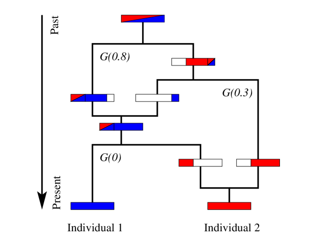
Figure 1: Illustration of the ancestral recombination graph of a contiguous locus for a sample of two individuals in the coalescent, after (Hudson, 1990). The locus is represented by the interval $[0,1]$, and $G(x)$ denotes the genealogy at position $x$. Two recombination events in the ancestral recombination graph, the more recent one at $x_{2}=0.8$ and the older one at $x_{1}=0.3$, partition the locus into three consecutive regions, $0\leq x<0.3$, $0.3\leq x<0.8$, and $0.8\leq x\leq 1$, with a different gene genealogy in each region [denoted $G(0)$, $G(0.3)$, and $G(0.8)$, respectively]. $G(0.3)$ is the genealogy resulting from taking the right branch in the first recombination event and the left branch in the second recombination event in the ancestral recombination graph. Similarly, the genealogy $G(0.8)$ corresponds to taking the rightmost branch in both recombination events.

This concludes our brief description of coalescent methods. Tab. 1 lists a number of different implementations of the coalescent algorithm. The first widely spread implementation was the ms program by (Hudson, 2002), and it is still one of the most widely used programs. In addition to the unstructured coalescent model, this implementation also supports simple models of population expansion and allows for sub-populations connected by migration. The extension of the coalescent framework to include different aspects of evolution is reflected in a large number of simulation programs which have emerged over the last few years (Tab. 1).

Program	Authors
ms	Hudson (2002)
SimCoal 2.0	Laval and Excoffier (2004)
SelSim	Spencer and Coop (2004)
CoaSim	Mailund et al. (2005)
CoSi	Schaffner et al. (2005)
SMC	McVean and Cardin (2005)
SMC’	Marjoram and Wall (2006)
FreGene	Hoggart et al. (2007)
Recodon	Arenas and Posada (2007)
Genome	Liang et al. (2007)
msHOT	Hellenthal and Stephens (2007)
GenomePop	Carvajal-Rodriguez (2008)

Table 1: Simulation packages for the coalescent (the list is not complete). Note that the ms package of Hudson (2002) is much older than the publication date indicates.

2.2 The sequential Markov coalescent method for an unstructured population

An important property of the coalescent process is that the marginal (single-locus) distribution of gene genealogies is independent of the position of the locus and thus independent of the recombination model (correlations between genealogies at different loci, by contrast, depend on the recombination model). Based on this observation, Wiuf and Hein (1999b, a) introduced an equivalent formulation of the coalescent process where the local gene-genealogical tree is followed along the chromosome, rather than tracing the ancestry of all loci back through time, as in the coalescent with recombination.

The procedure for generating the joint gene genealogies of a contiguous stretch of DNA is as follows: generate the genealogical tree corresponding to the left-most nucleotide of the stretch for all individuals in the sample. Let $T$ be the total length of this tree (the sum of the lengths of all branches in the tree), measured in generations. Generate the location of the next recombination event on the chromosome by moving an exponentially distributed number of nucleotides to the right. The expected value of the exponential distribution is $(rT)^{-1}$. If the location is beyond the right end of the stretch, the procedure terminates. If not, consider the genealogy for the nucleotides at the recombination location. Pick a point on this genealogy randomly uniformly. At this point (in time) the recombination event is assumed to occur. Trace a line starting from this point (the ‘recombination point’) back through time, and allow it merge with the ancestral recombination graph $G(x)$ with the standard coalescent rates. This new line is added to the ancestral recombination graph, the genealogy is updated, and correspondingly its total length $T$. In this way one continues to generate recombination events on the chromosome until the right end of the stretch is reached.

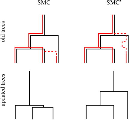
Figure 2: Illustration of the SMC and SMC’ approximations for a sample of three individuals. The top row shows the line re-attachment process. The given tree is drawn in black, the resulting tree using red lines. The re-attached line is dashed. In the SMC method, the line to be re-attached cannot be joined to its old path, whereas it can do so in the SMC’ method. The bottom row shows the resulting gene genealogies after the re-attachment process.

The method of Wiuf and Hein results in the same gene genealogies as the coalescent process. But it is also equally computationally demanding for large sample sizes and large genomic regions. To address this problem, McVean and Cardin (2005) sought an approximation to the method by Wiuf and Hein. As before, gene genealogies are constructed by moving along the chromosome (from left to right). When a recombination event occurs, the gene genealogy is updated. This update is illustrated in Fig. 2a. As usual, the recombination event causes one of the lines in the ancestral recombination graph to detach from the graph. The part of the line above the point of detachment (referred to as the recombination point in the preceding paragraph) is deleted from the ancestral recombination graph (see Fig. 2). Up to this step, the algorithm does not differ from the one proposed by Wiuf and Hein. The difference lies in the following simplification: instead of allowing the line to attach to any line of the ancestral recombination graph, it is only allowed to attach to lines in the local gene tree (see Fig. 2). It is thus no longer necessary to keep track of the full ancestral recombination graph. Hence, the work necessary to simulate a long contiguous stretch of DNA is significantly reduced compared to the coalescent process. The drawback of this simplification is that gene histories decorrelate faster as a function of the distance along the chromosome as compared with the exact coalescent process. The reason for this deviation lies in restricting the re-attachment process.

An improvement over the SMC method was suggested by Marjoram and Wall (2006). In their algorithm (SMC’ method) the line separated by a recombination event is allowed to attach also to its old path (see Fig. 2). While retaining the speed and memory efficiency of the SMC method, it was found to be significantly more accurate when compared to the exact coalescent process.

3 Methods

The SMC’ method in its original form (Marjoram and Wall, 2006) applies to unstructured populations with constant population size. In this section, we describe how the SMC’ method can be extended to models with population structure and changing population size. Figs. 3a-c show the three models for which we compare the standard coalescent to the SMC’ method. More complex models include combinations of population divergence and expansion, bottlenecks, and migration. As an example of such models, Fig. 3d depicts the out-of-Africa scenario for human history used by Schaffner et al. (2005), see also (Eriksson and Mehlig, 2004). Schaffner et al. (2005) implement a model of population structure, bottlenecks, and variable recombination rates along the chromosomes, tuned to match observed of allelic spectrums of different populations (African, Indo-European, Asian, and American).

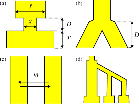
Figure 3: Scenarios of population history and structure. (a) Population bottleneck model. (b) The population-divergence model. (c) Two-island model. (d) A more complex scenario.

3.1 Bottleneck model

The population bottleneck model is illustrated in Fig. 3a. The population was of constant size $Ny$ until $2N(T+D)$ generations ago, when the population decreased to $Nx$ individuals during $2ND$ generations. After the bottleneck, the population quickly expanded to the present population size, $N$ individuals. It is straightforward to extend the SMC’ algorithm to this model. First, a gene genealogy for the leftmost locus is generated using the standard coalescent method for the model. Second, the position of the next recombination event is generated as in the SMC’ model. Third, the recombining line is re-attached using the same procedure as in the SMC’ method, but where the coalescent rate now depends on time, reflecting the changing population size.

3.2 Population divergence

Fig. 3b shows a model of population divergence. In this model, the population was of constant size of $N$ until $2ND$ generations ago, when it diverged into two parts with no gene flow between the two branches, which each grow to population size $N$. The branches may correspond to different species, or may correspond to sub-populations of the same species separated by e.g. a geographical barrier. If two individuals are sampled from the same branch, the population size is effectively constant. We therefore only consider the case where the individuals are sampled from different branches. In this case, the SMC’ algorithm is run separately for the two branches, from the present back to the time of the divergence. Some ancestral lines may merge during the divergence. The surviving ancestral lines are pooled in a single population, and the original SMC’ algorithm for constant population size is used to find the gene genealogies.

3.3 Island model

We consider the standard island model of population structure due to Wright (1931), see Fig. 3c. The population consists of two sub-populations, each with $N$ individuals, connected by a gene flow corresponding to $m$ migration events per generation. The scaled migration rate is $M=4Nm$.

The implementation of the SMC’ method in this model is more complicated than for the models of population bottlenecks and divergence shown in Fig. 3a and b. For this reason, the discussion in this subsection is restricted to sample size two (the algorithms described above apply to arbitrary sample sizes).

In contrast to the previous models, in the island model it is not sufficient to keep track of the total height of a genealogy in order to update the gene genealogies in the SMC’ algorithm. This is because the rate of attachment depends on the number of existing lines present in the island where the line to be attached resides. Hence, it is necessary to record also the sequence of migration events in the genealogy.

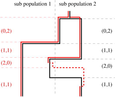
Figure 4: A sample genealogy of genes for the migration model in the $SMC^{\prime}$ algorithm. The black solid lines refer to the genealogy before recombination occurred, the red lines to the new genealogy. The re-attached line is drawn as a red dashed line. Also shown are the sequences of states, both according to the old and to the new genealogy (in black and red, respectively).

The re-attachment procedure for this population model is implemented as follows. First, let $n_{1}$ and $n_{2}$ be the number of ancestral lines sub populations 1 and 2, respectively ($n_{i}\in\{0,1,2\}$). Note that the variables $n_{i}$ are piecewise constant functions of time (Fig. 4). When a recombination event occurs, the breaking time (referred to as the recombination point above) is chosen uniformly randomly on the tree corresponding to the location of the recombination event. The detached line (the dashed line in Fig. 4) is re-attached to the old tree (black lines) applying standard rates of coalescence, and of migration between sub populations.

3.4 Gene-history correlations and probability of linkage

In order to compare the accuracy of the SMC’ approximation to the coalescent method, we study the correlation $\rho$ of the times to the most recent common ancestor for a sample of two individuals, at two loci separated by recombination rate $R$. This correlation underlies empirical measures of genetic variation, such as the variance of the number of segregating sites in a contiguous locus. Hence, if the models differ with respect to the correlation $\rho$, they are likely to differ also with respect to other observables (see, e.g. Hudson, 2001, for a review of properties of genetic variation in a sample which can be described by the two-locus statistics).

In the some population models, the correlation $\rho$ is found to be equal to the probability $p_{L}$ of linkage between the two loci in question. This is the case, for instance, in the constant population-size model and in the population-divergence model (but not in the population bottleneck and two-island models). In some cases (see below) we have been able to compute $p_{L}$ in closed form in the SMC’ approximation. The corresponding results are described in Sec. 4, but we first review the known results for the exact coalescent and for the SMC approximation.

For the constant population-size model, Hudson (1983) obtained the by now well-known exact result

$$p_{L}(R) =\rho(R)=\frac{R+18}{R^{2}+13R+18}\,.$$ (1)

Within the SMC approximation, the probability of linkage is found to be (McVean and Cardin, 2005)

$$p_{L}(R) =\frac{1}{1+R}.$$ (2)

Hence, in the simplest, constant population-size model, the exact probability of linkage and the one obtained within the SMC approximation are similar for small and large values of $R$. But they differ for intermediate values of $R$.

In the population-divergence model, the probability of linkage and the correlation can be calculated exactly using the method described in (Eriksson and Mehlig, 2004). One finds:

$$p_{L}(R)=\rho(R)=\frac{4(R^{2}+7R+18)}{(R+2)^{2}(R^{2}+13R+18)}\,\\ +\,\frac{8(R+6)R\,e^{-D(R+2)/2}+(R+10)R^{2}\,e^{-D(R+2)}}{(R+2)^{2}(R^{2}+13R+18)}.$$ (3)

It should be noted that this result differs from Eq. (14) in (Eriksson and Mehlig, 2004). The reason is that here we have conditioned on both individuals being in different sub populations at the present time, whereas the result in (Eriksson and Mehlig, 2004) was averaged over all four possibilities (both individuals in the same or in different sub populations).

4 Results

In this section we describe the results obtained when applying the SMC’ algorithm to the models of population structure described in Fig. 3a-c.

4.1 Population bottlenecks

In the population bottleneck model, the correlation $\rho$ differs from the probability of linkage $p_{L}$. Therefore we only study the former. Fig. 5 shows the correlation $\rho$ of the time to the most recent common ancestor for two loci separated by recombination rate $R$ in a sample of two individuals for the population bottleneck model [see Fig. 3a]. The correlation $\rho$ is shown as a function of the population size $x$ during the bottleneck. The symbols correspond to the SMC’ approximation, and the coloured lines to the coalescent algorithm. Results for three different recombination rates are shown: $R=0.5$ (green line, squares), $R=3.5$ (blue line, circles), and $R=15$ (red line, triangles). The other parameters are: $T=0.36$, $D=0.18$, and $y=1$.

Fig.  5 makes it clear that in the bottleneck model, the SMC’ approximation give very similar results to the coalescent. The largest deviations occur for relatively small widths of the bottleneck ($x\approx 0.1$) and for intermediate values of the recombination rate $R$.

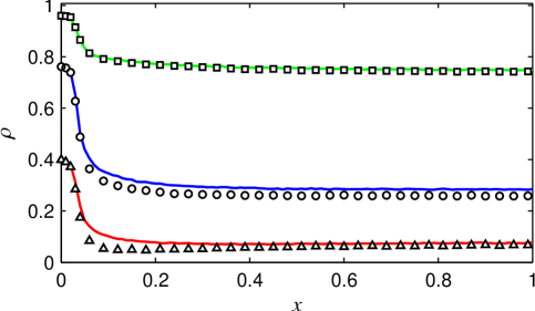
Figure 5: The correlation $\rho$ of the time to the most recent common ancestor for two loci separated by recombination rate $R$ in a sample of two individuals for the population bottleneck model (see Fig. 3a), for the SMC’ method (symbols) and the coalescent (colored lines), as a function of the population size $x$ during the bottleneck, for three recombination rates; $R=0.5$ (green line, squares), $R=3.5$ (blue line, circles), and $R=15$ (red line, triangles). The other parameters are: $T=0.36$, $D=0.18$, and $y=1$. All data points are calculated from simulations of $10^{6}$ independent realisations.

4.2 Population divergence model

Fig. 6 shows the correlation $\rho$ of the time to the most recent common ancestor for two loci separated by recombination rate $R$ for a sample of two individuals in the population-divergence model. Shown are the SMC’ approximation (symbols) and for the standard coalescent (solid lines), as a function of the recombination rate $R$ between the loci.

The upper panel shows how the correlation decrease as a function of $R$, for two values of the duration $D$ of the divergence. For $D=0$, corresponding to the standard constant population size, we confirm that the SMC’ approximation gives a correlation $\rho(R)$ which is very similar to that of the coalescent (blue solid line and circles). For $D=10$ (red solid line and triangles), however, SMC’ approxoimation differs significantly from the coalescent: the correlations decrease more rapidly in the SMC’ approximation than in the coalescent. While the correlations in the coalescent decrease as a power law, they decrease exponentially in the SMC’ approximation (as will be shown analytically below) when $D>0$. The largest differences occur for intermediate values of the recombination rate $R$.

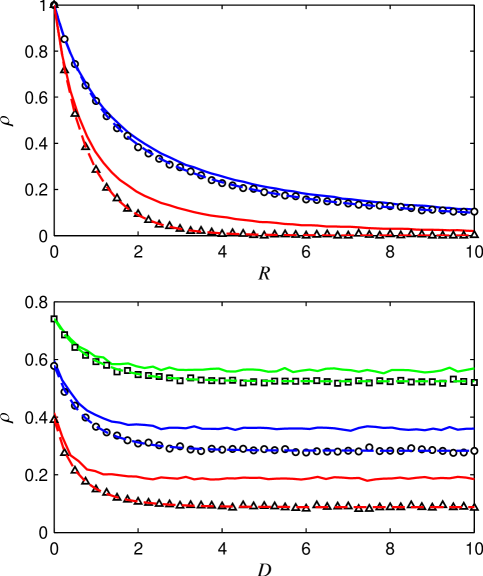
Figure 6: Top: the correlation $\rho$ of the time to the most recent common ancestor for two loci separated by recombination rate $R$ for a sample of two individuals in the population-divergence model (Fig. 3b); SMC’ approximation (symbols) and coalescent (lines), both as a function of the recombination rate $R$. All data points are calculated from simulations of $10^{\,5}$ independent realisations. The dashed lines represent the probability of linkage in the SMC’ model, Eq. (5). Two choices of the time $D$ since the divergence are shown: $D=0$ (no divergence, blue lines and circles), and $D=10$ (long divergence, red lines and triangles). Bottom: The correlation $\rho$ of the time to the most recent common ancestor of the two loci in the population-divergence model, for the SMC’ method (symbols) and the coalescent (lines), as a function of the duration $D$ of the divergence. All data points are calculated from simulations of $10^{5}$ independent realisations. Again, the dashed lines represent the probability of linkage in the SMC’ model. From top to bottom: $R=0.5$, $R=1$, and $R=2$.

A similar pattern can be seen in the lower panel, where the correlation $\rho$ is shown as a function of $D$ for different values of the recombination rate. The correlation is a decreasing function of $D$, but for large values of $D$ the decrease is very slow (we show below that the correlations approach a constant level for large values of $D$). For small values of $D$ the SMC’ approximation yields correlations $\rho$ which are close to those of the coalescent. The accuracy of the SMC’ approximation declines with increasing values of $D$, but for large values of $D$ the error approaches a constant.

It is very difficult to obtain an analytical expression for the correlation $\rho$ in the SMC’ approximation. However, a comparison in Fig. 6 of the probability of linkage $p_{L}$ to the correlation $\rho$ in the SMC’ approximation shows that, for the parameter values investigated, both appear to be identical (to within stochastic fluctuations).

In the following we show how to analytically calculate $p_{L}$. We first derive a general relation between the single-locus distribution function of the time $\tau$ to the most recent common ancestor, $f(\tau)$, and the probability of linkage, $p_{L}$. Let $\phi(\tau)$ be the probability that a line re-attaches to the same branch when started from a point uniformly on $[0,\tau]$. We refer to the probability $\phi(\tau)$ as the ‘loop probability’. Because the number of recombination events separating two loci is Poisson distributed, and since each recombination event leaves the genealogy intact with probability $\phi(\tau)$, we find that the probability of linkage is

$$p_{L}(R) =\int_{0}^{\infty}d\tau\,f(\tau)\sum_{k=0}^{\infty}[\phi(\tau)]^{k}\frac{(R\tau)^{k}}{k!}e^{-R\tau}$$

$$=\int_{0}^{\infty}d\tau\,f(\tau)\,e^{-[1-\phi(\tau)]R\tau}.$$ (4)

Thus, in order to obtain the probability of linkage for a given population model, one needs to calculate the loop probability.

In Appendix A we summarise this calculation for the population divergence model (and, as a special case, for a freely mixing population of constant size). The result is:

$$p_{L} =\frac{e^{-R/2}}{2}\int_{0}^{1}ds\,s^{(R-2)/4}\exp\left[-\frac{R(1-2e^{-D})(1+s)}{4}\right]\,.$$ (5)

This result can be expressed in closed form in terms of the incomplete Gamma function (see Appendix A for details). In Appendix A.2.1 we derive a bound for this probability:

$$p_{L} \leq\frac{8e^{-(3-2e^{-D})R/4}}{R^{2}+8R+12}+\frac{2e^{-(1-e^{-D})R}}{R+6}\,.$$ (6)

Eq. (6) shows that the linkage probability falls off exponentially with increasing $R$ for all values of $D>0$. Now consider the exact probability of linkage in the coalescent algorithm, Eq. (3). According to this expression, $p_{L}$ falls off at a rate $\sim 4/R^{2}$ when $RD\gg 1$, and not exponentially as in the SMC’ approximation.

Note, however, that when $D=0$ (corresponding to a freely mixing population of constant size), the bound (6) for $p_{L}$ in the SMC’ approximation does not decrease exponentially but as $2/(R+6)$ for large values of $R$. A lower bound for this case, $p_{L}\geq 1/(1+R)$, is derived in Appendix A.2.2 and confirms that for $D=0$ the probability of linkage decreases inversely proportional to $R$.

In summary, for the population divergence model we have found the following. For sufficiently large duration of the divergence (for a large value of $D$), there may be significant differences in the correlation $\rho$ between the coalescent and the SMC’ approximation. The main reason for this discrepancy is that in the coalescent, the ancestral lines may merge and break several times during the divergence, but in the SMC’ approximation the probability this to happen is much lower. In addition, we have established numerically that in the SMC’ approximation, the correlation $\rho$ and the probability of linkage appear to be identical (this is known to strictly hold in the coalescent, c.f. the discussion in the methods section). Last but not least, our analytical results within SMC’ approximation show that the probability of linkage decreases exponentially with increasing recombination rate, in contrast the exact coalescent where the probability of linkage decreases as a power law in $R$.

4.3 Two-island model

In Fig. 7 we show the correlation $\rho$ of the time to the most recent common ancestor for two loci separated by recombination rate $R$ in a sample of two individuals for the two-island model (Fig. 3c), as function of $R$ for three different migration rates: $M=0.01$ (green line and triangles), $M=0.2$ (blue line and circles), and $M=10$ (red line and diamonds). The results are based on $10^{4}$ simulations of the standard two-island coalescent with migration, and the two-island extension of the SMC’ method described in Section 4.3.

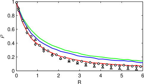
Figure 7: Correlation $\rho$ of the time to the most recent common ancestor for two loci separated by recombination rate $R$ in a sample of two individuals for the two-island model (see Fig. 3c), as function of $R$ for $M=0.01$ (green line and triangles), $M=0.2$ (blue line and circles), and $M=10$ (red line and diamonds). The lines corresponds to from simulations of the coalescent, and the symbols to simulations of the SMC’ model, from $10^{4}$ independent realisations.

When the migration rate is large, the SMC’ approximation gives results very similar to those of the coalescent. This is expected since in this case the population behaves as a single panmictic unit. For intermediate and small migration rates, however, differences are observed. These differences increase with decreasing migration rates.

5 Discussion

In this article we have investigated the accuracy of the SMC’ approximation to the coalescent for the population models depicted in Fig. 3a-c. This is an important question since many populations show deviations in their allelic distributions consistent with historic population expansions, bottlenecks, and structure from geographic separation or preferential mating. To determine the accuracy we have computed the correlation of the time to the most recent common ancestor for two loci in a sample of two individuals in the SMC’ approximation. We have compared these results to the corresponding exact coalescent results. In this section we briefly discuss the results for the three different models, and put them in a wider context.

In the population-bottleneck model (Fig. 3a) we have found that the SMC’ approximation works well. This result can be understood more generally as follows. Consider a general model of time-dependent population-size variations, where $N(t)$ is the population size as a function of time. The coalescent for this model can be mapped to the constant population-size model by introducing a (possibly nonlinear) transformation of the time $\tau$ to a ‘stretched’ time

$$\tau^{\prime}=\int_{0}^{\tau}{\rm d}t\,N(0)/N(t)\,.$$ (7)

Because of the construction of the SMC’ algorithm, the coalescent and the corresponding SMC’ approximation are transformed in the same way by this transformation. Hence, it may be expected that the SMC’ approximation works well for arbitrary models of population expansions and bottlenecks. We have verified this expectation for the particular case of the bottleneck model depicted in Fig. 3a.

In the population-divergence model (Fig. 3b) the situation is different. We have calculated the linkage probability $p_{L}$ (which is equal to $\rho$ in this model) both exactly and within the SMC’ approximation of the coalescent. Our analytical results show that when the expected number of recombination events during the divergence becomes large, the accuracy of the SMC’ approximation deteriorates: the exact correlation decreases as a power law as a function of $R$, whereas in the SMC’ approximation it decreases exponentially.

In order to better understand this difference, let us compare how the divergence affects the gene genealogies in the coalescent to how it affects gene genealogies in the SMC’. In the coalescent, recombination can cause the genetic material to spread out over different ancestral lines during the divergence. The probability of linkage depends on whether the genetical material is spread over two, three or four lines at the onset of the divergence. In each case, however, the coalescent results in a probability of linkage which decreases as a power law with increasing $R$.

In the SMC’ approximation, by contrast, the probability of linkage is a function of the loop probability. As explained in Section 4.2, the cause of the exponential decrease of the probability of linkage in the SMC’ approximation can be traced back to how the loop probability depends on the duration of the divergence. Hence, the different behaviours of the coalescent and the SMC’ approximation can be attributed to the lack of memory of past gene genealogies within the SMC’ approximation.

Note also that if there is a severe population bottleneck during the divergence, we expect that the differences between the coalescent and the SMC’ will be smaller, since the bottleneck increases the chances that the genes will be linked right before the divergence. This means that as far as the correlation of times to the most recent common ancestor is concerned, bottlenecks right after the divergence have the same effect as decreasing the time $D$ to the divergence.

The third model we have considered is the two-island model with migration (Fig. 3c). The extension of the SMC’ approximation to this model turned out to be more complicated than in the other two models, since it is necessary to keep track of not only the time to the most recent common ancestor in the genealogy, but also of the sequence of migration events. Simulations of the exact coalescent and the SMC’ approximation showed that when the migration rate is large, the SMC’ approximation is accurate. For small and intermediate values of the migration rate, by contrast, significant differences were found. The magnitude of the relative deviations between the exact result and the SMC’ approximation is similar to those in the population divergence model. Numerical analysis shows that when the recombination rate $R$ between the two loci is sufficiently large, $\rho$ decreases exponentially with increasing $R$ in the SMC’, whereas in the coalescent it is approximately inversely proportional to $R$ in this regime.

It follows from our results that in a more complex scenario such as that depicted in Fig. 3d, one may expect the SMC’ approximation to work well when individuals are sampled from the same sub population. When the individuals are sampled from different geographical locations, however, or more generally when one may expect reduced gene flow between the different sample locations, the accuracy of the SMC’ needs to be carefully investigated. We have found that the accuracy depends upon the amount of gene flow within and between sub populations, on how recently divergences may have occurred, and upon the genetic distance between the loci in question. These dependencies are summarised in Figs. 5, 6, and 7.

Acknowledgments. We acknowledge support from Vetenskapsrådet and from the Centre for Theoretical Biology at Gothenburg University.

Appendix A Probability of linkage

In this appendix we summarise how to calculate the probability of linkage in the SMC’ approximation, for a freely mixing population of constant size, and for the population-divergence model. We begin by discussing the constant population-size model, and then turn to the population divergence.

A.1 Constant population size

Consider a freely mixing population of constant size. To determine the linkage probability of two loci in a sample of size two, the first step is to calculate the loop probability $\phi(\tau)$, the probability that the detached line re-attaches to the line it originated from before the two lines in the genealogy coalesce at time $\tau$ (upper right panel of Fig. 2). Suppose that the recombination point occurs at time $t$ (with $0<t<\tau$). Since there are two lines to attach to, the time to attachment is exponentially distributed with rate two. Given that the line attaches before time $\tau$, it attaches to the original line with probability $1/2$. Hence, the probability of a loop occuring from recombination point at time $t$ is

$$\frac{1}{2}\int_{t}^{\tau}dt^{\prime}2e^{-2(t^{\prime}-t)}.$$

In SMC’ approximation, the recombination point $t$ is chosen from a uniform distribution over the gene genealogy. Hence, the probability that a recombination event re-attaches to the same line and thus leaves the gene genealogy intact (this is the loop probability) is found by averaging over all recombination points $t\in[0,\tau]$:

$$\phi(\tau) =\frac{1}{\tau}\int_{0}^{\tau}dt\,\frac{1}{2}\int_{t}^{\tau}dt^{\prime}2e^{-2(t^{\prime}-t)}=\frac{2\tau-1+e^{-2\tau}}{4\tau}\,.$$ (8)

In the second step, we use the loop probability (8) in combination with the distribution of the time to the most recent common ancestor for a single locus to calculate the probability of linkage. In a freely mixing population of constant size, the time to the most recent common ancestor is exponentially distributed with unit mean,

$$f(\tau) =e^{-\tau}\,.$$ (9)

Inserting Eqs. (8) and (9) into the general formula, Eq. (4), results in:

$$p_{L}(R) =\int_{0}^{\infty}d\tau\exp\Big{[}\!-\tau-\left(2\tau+1-e^{-2\tau}\right)R/4\Big{]}$$

$$=\frac{1}{2}\int_{0}^{1}ds\,s^{(R-2)/4}e^{-R(1-s)/4}$$

$$=2^{R/2}\,e^{-R/4}\,(-R)^{-(R-2)/4}\,\gamma\Big{(}(R+2)/4,-R/4\Big{)}\,.$$ (10)

Here $\gamma$ is the so-called ‘lower incomplete Gamma function’ defined as $\gamma(a,b)=\int_{0}^{b}{\rm d}t\,t^{a-1}{\rm e}^{-t}$. Eq. (A.1) is our result for the probability of linkage for two loci in a sample of two individuals for a freely mixing population of constant size in the SMC’ approximation.

A.2 Population divergence model

For the case of a population divergence, the calculation is complicated by the difference in population structure during different stages of the history. We assume that the two individuals are sampled from different sub-populations, so that the most recent common ancestor occurred before the divergence. The time to the most recent common ancestor for the left-most locus has a shifted exponential distribution:

$$f(\tau)=\left\{\begin{array}[]{ll}e^{-(\tau-D)}&\mbox{for $\tau>D$}\\ 0&\mbox{otherwise}\,.\end{array}\right.$$ (13)

If recombination and re-attachment occur during the divergence the result must be a loop, because the line corresponding to the other individual resides in the other sub-population. If recombination or re-attachment do not occur during the divergence, the re-attachment process is the same as in Sec. A.1: the line attaches with rate $2$ until the most recent common ancestor is reached.

Let $\psi(t,\tau)$ be the probability of a loop occuring, where $t$ is the time of the recombination event and $\tau$ is the time of the most recent common ancestor. First, consider the case of $t<D$. During the interval $[t,D]$, the line re-attaches to the ancestral recombination graph with rate one, and if it re-attaches it is to the original line it detached from. Within the time interval $[D,\tau]$, the line re-attaches with rate 2, and the probability that the re-attachment point is on the original line is $1/2$. This gives the contribution

$$\psi(t,\tau) =1-e^{-(D-t)}+\frac{1}{2}e^{-(D-t)}\left[1-e^{-2(\tau-D)}\right]$$ (14)

to the loop probability. When the recombination point is before the divergence ($D<t<\tau$), we obtain

$$\psi(t,\tau) =\frac{1}{2}\left[1-e^{-2(\tau-t)}\right]$$ (15)

using the same arguments as for $t<D$. Since the starting point is chosen uniformly from the gene genealogy, the loop probability $\phi(\tau)$ is

$$\phi(\tau) =\frac{1}{\tau}\int_{0}^{\tau}dt\,\psi(t,\tau)$$

$$=\frac{2(D+\tau)-3+2e^{-D}-\left(1-2e^{-D}\right)e^{-2(\tau-D)}}{4\tau}\,.$$ (16)

We insert Eqs. (13) and (A.2) into the general expression for the loop probability, Eq. (4). Further, we perform a change of integration variable from $\tau$ to $s=\exp[-2(\tau-D)]$. This leads to Eq. (5).

A.2.1 Upper bound for $p_{L}$

We now show how the bound (6) was obtained. We make use of the fact that the exponential function is convex and obtain the following inequality valid for $0\leq s\leq 1$, with equality only at the end points:

$$e^{-R(1-2e^{-D})(1+s)/4} \leq e^{-R(1-2e^{-D})/4}(1-s)+e^{-R(1-2e^{-D})/2}s\,.$$ (17)

Inserting this expression into Eq. (5) results in Eq. (6). Plotting the right-hand side and comparing to the exact integral in Eq. (5) shows that the inequality Eq. (6) is very close to being an equality for the parameters used in Fig. 6.

A.2.2 Lower bound for $p_{L}$ at $D=0$

For $D=0$, the upper bound does not decrease exponentially with $R$, but in order to say that $p_{L}$ does not decrease exponentially we need a lower bound. We can obtain one such by writing (A.1) as

$$p_{L}=\frac{1}{2}\int_{0}^{1}dt\,(1-t)^{(R-2)/4}e^{-Rt/4}\,.$$ (18)

Using the inequality $e^{-\alpha t}\geq(1-t)^{\alpha}$, which is valid for all $\alpha\geq 0$ and $0\leq t\leq 1$, we obtain

$$p_{L}\geq\frac{1}{2}\int_{0}^{1}dt\,(1-t)^{(R-1)/2}=\frac{1}{1+R}$$ (19)

which we recognize as the probability of linkage in the SMC model. From this bound it is clear that $p_{L}$ decreases as $1/R$ for large values of $R$, rather than decreasing exponentially as the exact result does, compare Eqs. (3) and (6).

References

- Altshuler et al. (2005) Altshuler, D., Brooks, L., Chakravarti, A., Collins, F., Daly, M., Donnelly, P., 2005. A haplotype map of the human genome. Nature 437 (7063), 1299–1320.
- Arenas and Posada (2007) Arenas, M., Posada, D., 2007. Recodon: Coalescent simulation of coding dna sequences with recombination, migration and demography. BMC Bioinformatics 8, 458.
- Carvajal-Rodriguez (2008) Carvajal-Rodriguez, A., 2008. Genomepop: A program to simulate genomes in populations. BMC Bioinformatics 9, 223.
- Coop and Griffiths (2004) Coop, G., Griffiths, R. C., 2004. Ancestral inference on gene trees under selection. Theor. Popul. Biol. 66, 219–232.
- Eriksson et al. (2007) Eriksson, A., Fernström, P., Mehlig, B., Sagitov, S., 2007. An accurate model for genetic hitch-hiking. Genetics 178, 1–13.
- Eriksson and Mehlig (2004) Eriksson, A., Mehlig, B., 2004. Gene-history correlation and population structure. Physical Biology 1, 220–228.
- Eriksson and Mehlig (2005) Eriksson, A., Mehlig, B., 2005. On the effect of fluctuating recombination rates on the decorrelation of gene histories in the human genome. Genetics 169, 1175–1178.
- Golding (1984) Golding, G. B., 1984. The sampling distribution of linkage disequilibrium. Genetics 108, 257–274.
- Griffiths (1981) Griffiths, R. C., 1981. Neutral 2-locus multiple allele models with recombination. Theor. Pop. Biol. 19, 169–186.
- Hellenthal and Stephens (2007) Hellenthal, G., Stephens, M., 2007. mshot: modifying hudson’s ms simulator to incorporate crossover and gene conversion hotspots. Bioinformatics 23 (4), 520–521.
- Hoggart et al. (2007) Hoggart, C. J., Chadeau-Hyam, M., Clark, T. G., Lampariello, R., Whittaker, J. C., De Iorio, M., Balding, D. J., 2007. Sequence-level population simulations over large genomic regions. Genetics 177 (3), 1725–1731.
- Hudson (1983) Hudson, R. R., 1983. Properties of a neutral allele model with intragenic recombination. Theoretical Population Biology 23, 183–201.
- Hudson (1990) Hudson, R. R., 1990. Gene genealogies and the coalescent process. In: Futuyma, D., Antonovics, J. (Eds.), Oxford Surveys in Evolutionary Biology. Oxford University Press, Oxford, pp. 1–43.
- Hudson (2001) Hudson, R. R., 2001. Two-locus sampling distributions and their application. Genetics 159, 1805–1817.
- Hudson (2002) Hudson, R. R., 2002. Generating samples under a Wright-Fisher neutral model of genetic variation. Bioinformatics 18 (2), 227–338.
- Hudson and Kaplan (1988) Hudson, R. R., Kaplan, N. L., 1988. The coalescent process in models with selection and recombination. Genetics 120, 831–840.
- Kaplan et al. (1989) Kaplan, N. L., Hudson, R. R., Langley, C. H., 1989. The “hitchhiking effect” revisited. Genetics 123, 887–899.
- Kingman (1982) Kingman, J. F. C., 1982. On the genealogy of large populations. Journal of Applied Probability 19A, 27–43.
- Kong et al. (2002) Kong, A., Gudbjartsson, D. F., Sainz, J., Jonsdottir, G. M., Gudjonsson, S. A., Richardsson, B., Sigurdardottir, S., Barnard, J., Hallbeck, B., Masson, G., Shlien, A., Palsson, S. T., Frigge, M. L., Thorgeirsson, T. E., Gulcher, J. R., Stefansson, K., 2002. A high-resolution recombination map of the human genome. Nature 31, 241–247.
- Krone and Neuhauser (1997) Krone, S. M., Neuhauser, C., 1997. Ancestral processes with selection. Theoretical Population Biology 51, 210–237.
- Laval and Excoffier (2004) Laval, G., Excoffier, L., 2004. Simcoal 2.0: a program to simulate genomic diversity over large recombining regions in a subdivided population with a complex history. Bioinformatics 20 (15), 2485–2487.
- Liang et al. (2007) Liang, L., Zollner, S., Abecasis, G. R., 2007. Genome: a rapid coalescent-based whole genome simulator. Bioinformatics 23 (12), 1565–1567.
- Liang and Kelemen (2008) Liang, Y., Kelemen, A., 2008. Statistical advances and challenges for analyzing correlated high dimensional snp data in genomic study for complex diseases. Statistics Surveys 2, 43–60.
- Lindblad-Toh et al. (2000) Lindblad-Toh, K., Winchester, E., Daly, M. J., Wang, D. G., Hirschhorn, J. N., Laviolette, J.-P., Ardlie, K., Reich, D. E., Robinson, E., Sklar, P., Shah, N., Thomas, D., Fan, J.-B., Gingeras, T., Warrington, J., Patil, N., Hudson, T. J., Lander, E. S., 2000. Large-scale discovery and genotyping of single-nucleotide polymorphisms in the mouse. Nature Genetics 24, 381–386.
- Mailund et al. (2005) Mailund, T., Schierup, M. H., Pedersen, C. N. S., Mechlenborg, P. J. M., Madsen, J. N., Schauser, L., 2005. Coasim: a flexible environment for simulating genetic data under coalescent models. BMC Bioinformatics 6, 252.
- Marjoram and Tavare (2006) Marjoram, P., Tavare, S., 2006. Modern computational approaches for analysing molecular genetic variation data. Nature Reviews Genetics 7 (10), 759–770.
- Marjoram and Wall (2006) Marjoram, P., Wall, J., 2006. Fast ”coalescent” simulation. BMC Genetics 7, 16.
- McVean and Cardin (2005) McVean, G. A. T., Cardin, N. J., 2005. Approximating the coalescent with recombination. Phil. Trans. R. Soc. B 360, 1387–1393.
- Nordborg (2001) Nordborg, M., 2001. Coalescent theory. In: Balding, D. J., Bishop, M., Cannings, C. (Eds.), Handbook of Statistical Genetics. John Wiley & Sons, Ch. 7, pp. 179–212.
- Nordborg et al. (2005) Nordborg, M., Hu, T., Ishino, Y., Jhaveri, J., Toomajian, C., Zheng, H., Bakker, E., Calabrese, P., Gladstone, J., Goyal, R., Jakobsson, M., Kim, S., Morozov, Y., Padhukasahasram, B., Plagnol, V., Rosenberg, N., Shah, C., Wall, J., Wang, J., Zhao, K., Kalbfleisch, T., Schulz, V., Kreitman, M., Bergelson, J., 2005. The pattern of polymorphism in arabidopsis thaliana. Plos Biology 3 (7), 1289–1299.
- Patterson et al. (2006) Patterson, N., Richter, D. J., Gnerre, S., Lander, E. S., Reich, D., 2006. Genetic evidence for complex speciation of humans and chimpanzees. Nature 441, 1103–1108.
- Przeworski (2002) Przeworski, M., 2002. The signature of positive selection at randomly chosen loci. Genetics 160, 1179 – 1189.
- Sano et al. (2004) Sano, A., Shimizu, A., Iizuka, M., 2004. Coalescent process with fluctuating population size and its effective size. Theor. Pop. Biol. 65, 39–48.
- Schaffner et al. (2005) Schaffner, S., Foo, C., Gabriel, S., Reich, D., Daly, M., Altshuler, D., 2005. Calibrating a coalescent simulation of human genome sequence variation. Genome Research 15 (11), 1576–1583.
- Slatkin and Hudson (1991) Slatkin, M., Hudson, R. R., 1991. Pairwise comparisons of mitochondrial dna sequences in stable and exponentially growing populations. Genetics 129, 555–562.
- Spencer and Coop (2004) Spencer, C. C. A., Coop, G., 2004. Selsim: a program to simulate population genetic data with natural selection and recombination. Bioinformatics 20 (18), 3673–3675.
- Stumpf and Goldstein (2003) Stumpf, M. P. H., Goldstein, D. L., 2003. Demography, recombination hotspot intensity, and the block structure of linkage disequilibrium. Curr. Biol.. 13, 1–8.
- Tajima (1989a) Tajima, F., 1989a. The effect of change in population size on dna polymorphism. Genetics 123, 597–601.
- Tajima (1989b) Tajima, F., 1989b. Statistical method for testing the neutral mutation hypothesis by DNA polymorphism. Genetics 123, 585–595.
- Teshima and Tajima (2003) Teshima, K. M., Tajima, F., 2003. The effect of migration during the divergence. Theor. Pop. Biol. 62, 81–95.
- The International HapMap Consortium (2007) The International HapMap Consortium, 2007. A second generation human haplotype map of over 3.1 million SNPs. Nature 449 (7164), 851–U3.
- Wakeley (1996) Wakeley, J., 1996. The variance of pairwise nucleotide differences in two populations with migration. Theor. Pop. Biol. 49, 39–57.
- Wiuf and Hein (1999a) Wiuf, C., Hein, J., 1999a. The ancestry of a sample of sequences subject to recombination. Genetics 151, 1217–1228.
- Wiuf and Hein (1999b) Wiuf, C., Hein, J., 1999b. Recombination as a point process along sequences. Theor. Pop. Biol. 55, 248–259.
- Wiuf and Posada (2003) Wiuf, C., Posada, D., 2003. A coalescent model of recombination hotspots. Genetics 164, 407–417.
- Wright (1931) Wright, S., 1931. Evolution in Mendelian populations. Genetics 16 (2), 97–159.
- Yu and Buckler (2006) Yu, J., Buckler, E., 2006. Genetic association mapping and genome organization of maize. Current Opinion In Biotechnology 17 (2), 155–160.