The ground state magnetic phase diagram of the ferromagnetic Kondo-lattice model

Abstract

The magnetic ground state phase diagram of the ferromagnetic Kondo-lattice model is constructed by calculating internal energies of all possible bipartite magnetic configurations of the simple cubic lattice explicitly. This is done in one dimension (1D), 2D and 3D for a local moment of $S=\frac{3}{2}$. By assuming saturation in the local moment system we are able to treat all appearing higher local correlation functions within an equation of motion approach exactly. A simple explanation for the obtained phase diagram in terms of bandwidth reduction is given. Regions of phase separation are determined from the internal energy curves by an explicit Maxwell construction.

I Introduction

The ferromagnetic Kondo lattice model (FKLM), also referred to as $s$-$d$ model or double exchange model, is the basic model for understanding magnetic phenomena in systems where local magnetic moments couple ferro-magnetically to itinerant carriers. This holds for a wide variety of materials.

In the context of transition metal compounds Zener proposed the double exchange mechanism to explain ferromagnetic (FM) metallic phase in the manganites Zener (1951a, b). In these materials the Mn $5d$ shells are split by the crystal field into three degenerate $t_{2g}$ orbitals which are localized and form a total spin $S=\frac{3}{2}$ according to atomic selection rules and two $e_{g}$ orbitals providing the itinerant electrons. These electrons couple via Hund exchange coupling ferro magnetically with the localized spins. Therefore the FKLM is a basic ingredient to describe the rather complex physics of the manganites Dagotto (2003); Stier and Nolting (2007, 2008).

Another nearly ideal field of application of the FKLM is the description of the rare earth materials Gd and EuX (X=O,S,Se,Te). These materials have a half filled $4f$ shell in common that is strongly localized and the electrons in this shell couple to a total spin momentum of $S=\frac{7}{2}$. The FKLM was then used successfully to explain the famous redshift of the absorption edge of the optical $4f$-$5d$ transition in the ferromagnetic semiconductor EuOBusch et al. (1964); Rys et al. (1967). In [Santos et al., 2004] a many-body analysis of the FKLM in combination with a band structure calculation was used to get a realistic value for the Curie temperature of the ferromagnetic metal Gd that is in good agreement with experiment.

Although it is necessary to extent the FKLM in order to get a realistic description of the above mentioned examples knowledge of the properties of the pure (single band) FKLM is crucial for understanding these materials.

To reveal the ground state magnetic phases one has to solve the many-body problem of the FKLM. This was already done in previous works by using different techniques. Dynamical mean field theory (DMFT) was used by several authors [Yunoki et al., 1998; Kagan et al., 1999; Chattopadhyay et al., 2001; Lin and Millis, 2005] to get information about different magnetic domains. In [Pekker et al., 2005] a continuum field theory approach was used to derive the 2D phase-diagram at $T=0$. Classical Monte Carlo simulations were performed in [Yunoki et al., 1998; Dagotto et al., 1998]. For 1D systems numerical exact density-matrix renormalization group calculations were done in [Garcia et al., 2004]. In [Kienert and Nolting, 2006] the authors have used a Green function method to test the validity of assuming the quantum localized spins to be classical objects. Extended FKLMs including more material specific effects were for instance investigated in [Peters and Pruschke, 2007; Stier and Nolting, 2008].

In this work we will compare all bipartite magnetic configurations for the simple cubic (sc) lattice by calculating their respective internal energies. To this end the electronic Green function has to be determined. This is done by an equation of motion approach and, assuming that the local moment system is saturated, we are able to show that all appearing local higher correlation functions can be treated exactly. From the calculated internal energies the phase-diagram is constructed and region of phase-separation are determined.

The paper is organized as follows. In Sec. II the model Hamiltonian and details of the calculation are presented. In Sec. III we discuss the phase-diagrams and give an explanation for the sequence of phases obtained by looking at the quasi-particle density of states. In Sec. IV we summarize the results and give an outlook on possible directions for further research.

II Model and Theory

II.1 Model Hamiltonian

For a proper description of different (anti-) ferromagnetic alignments of localized magnetic moments it is useful to divide the full lattice into two or more sub-lattices (primitive cells) each ordering ferro magnetically.
In this work we only consider simple cubic bipartite lattices, i.e. anti-ferromagnetic configurations that can be obtained by dividing the simple cubic lattice into two sub-lattices. In Fig.(1) all possible decompositions in two and three dimensions are shown. In case of 1D only the ferromagnetic and g-type anti-ferromagnetic phase remain.

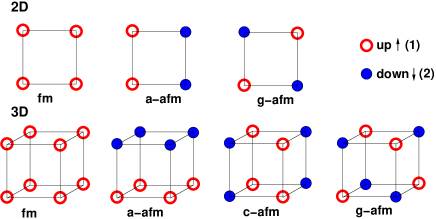
Figure 1: (Color online) Magnetic phases considered in this work (1D omitted).

The Hamiltonian of the FKLM in second quantization reads as follows:

$$H=H_{s}+H_{sf}=\sum_{ij\sigma}\sum_{\alpha\beta}T^{\alpha\beta}_{ij}c^{+}_{i\alpha\sigma}c_{j\beta\sigma}$$ (1)

$$-\frac{J}{2}\sum_{i\sigma}\sum_{\alpha}\left(z_{\sigma}S^{z}_{i\alpha}c^{+}_{i\alpha\sigma}c_{i\alpha\sigma}+S^{\sigma}_{i\alpha}c^{+}_{i\alpha-\sigma}c_{i\alpha\sigma}\right).$$

The first term describes the hopping of Bloch electrons with spin $\sigma$ between different sites. The lattice sites $\mathbf{R}_{i\alpha}$ are denoted by a Latin index $i$ for the unit cell and an Greek index $\alpha\in{A,B}$ for the corresponding sub-lattice, i.e. $\mathbf{R}_{i\alpha}=\mathbf{R}_{i}+\mathbf{r}_{\alpha}$. The second term describes a local Heisenberg-like exchange interaction between the itinerant electrons and local magnetic moments $\mathbf{S}_{i\alpha}$ where $J>0$ is the strength of this interaction, $z_{\uparrow\downarrow}=\pm 1$ accounts for the two possible spin projections of the electrons and ($S^{\sigma}_{i\alpha}=S^{x}_{i\alpha}+z_{\sigma}iS^{y}_{i\alpha}$) denotes the spin raising/lowering operator.

II.2 internal energy

The internal energy of the FKLM at $T=0$ is given by ground state expectation value of the Hamiltonian:

$$U=\langle H\rangle=\frac{1}{2}\sum_{\alpha\sigma}\int_{-\infty}^{\infty}f_{-}(E)ES_{\alpha\sigma}(E)dE$$ (2)

where $S_{\alpha\sigma}(E)=-\frac{1}{\pi}\mathrm{Im}G_{\alpha\sigma}(E)$ is the local spectral density, $f_{-}(E)$ denotes the Fermi function and $G_{\alpha\sigma}(E)$ denotes the local electronic Green function (GF). Note, that this formula is obtained by a straightforward calculation of the ground-state expectation value of the Hamiltonian (1) using the spectral theorem and is therefore exact.

Our starting point is the equation of motion (EQM) for the electronic GF:

$$\sum_{l\gamma}\left(E\delta^{\alpha\gamma}_{il}-T^{\alpha\gamma}_{il}\right)G^{\gamma\beta}_{lj\sigma}=\delta^{\alpha\beta}_{ij}-\frac{J}{2}\left(I^{\alpha\alpha\beta}_{iij\sigma}+F^{\alpha\alpha\beta}_{iij\sigma}\right)$$ (3)

with Ising-GF: $I^{\alpha\gamma\beta}_{ikj\sigma}=z_{\sigma}\langle\!\langle S^{z}_{i\alpha}c_{k\gamma\sigma};c^{+}_{j\beta\sigma}\rangle\!\rangle$ and spin-flip-GF: $F^{\alpha\gamma\beta}_{ikj\sigma}=\langle\!\langle S^{-\sigma}_{i\alpha}c_{k\gamma-\sigma};c^{+}_{j\beta\sigma}\rangle\!\rangle$. Our basic assumption for the ground state is perfect saturation of the local moment system . With this assumption the Ising-GF can be decoupled exactly:

$$I^{\alpha\gamma\beta}_{ikj\sigma}(E)\rightarrow z_{\sigma}z_{\alpha}SG^{\gamma\beta}_{kj}(E)$$ (4)

where $z_{\alpha}=\pm 1$ denotes the direction of sub-lattice magnetization. In a first attempt to solve Eq. (3) we have neglected spin-flip processes completely ($F^{\alpha\gamma\beta}_{ikj\sigma}\approx 0$). With (4) we then get a closed system of equations which can be solved for the electronic GF by Fourier transformation:

$$G^{(\mathrm{MF})}_{\alpha\sigma}(E) = \frac{1}{N}\sum_{\mathbf{q}}G^{\alpha\alpha(\mathrm{MF})}_{\mathbf{q}\sigma}(E)$$

$$= \frac{1}{N}\sum_{\mathbf{q}}\frac{1}{E+z_{\sigma}z_{\alpha}\frac{J}{2}S-\epsilon^{\alpha\alpha}_{\mathbf{q}}-\frac{\epsilon^{\alpha\bar{\alpha}}_{\mathbf{q}}\epsilon^{\bar{\alpha}\alpha}_{\mathbf{q}}}{E+z_{\sigma}z_{\bar{\alpha}}\frac{J}{2}S-\epsilon^{\bar{\alpha}\bar{\alpha}}_{\mathbf{q}}}}$$

where $\epsilon^{\alpha\beta}_{\mathbf{q}}$ is the Fourier transform of the hopping integral and $\bar{\alpha}=-\alpha$ denotes the complementary sub-lattice. We will call this solution the “mean-field” (MF) solution. Note, that the ferromagnetic phase is contained in the above formula by setting $\epsilon^{\alpha\bar{\alpha}}_{\mathbf{q}}$ to zero.

To go beyond the MF treatment it is necessary to find a better approximation for the spin-flip-GF. To this end we write down the EQM for the spin-flip-GF:

$$\sum_{l\mu}\left(E\delta^{\gamma\mu}_{kl}-T^{\gamma\mu}_{kl}\right)F^{\alpha\mu\beta}_{ilj\sigma}=$$

$$\langle\!\langle\left[S^{-\sigma}_{i\alpha},H_{sf}\right]_{-}c_{k\gamma-\sigma};c^{+}_{j\beta\sigma}\rangle\!\rangle+\langle\!\langle S^{-\sigma}_{i\alpha}\left[c_{k\gamma-\sigma},H_{sf}\right]_{-};c^{+}_{j\beta\sigma}\rangle\!\rangle$$

Our strategy to get an approximate solution for the spin-flip-GF is to treat the non-local correlations on a mean-field level whereas the local terms will be treated more carefully. This is similar to the idea of the dynamical mean field theory (DMFT) developed for strongly correlated electron systems.Georges et al. (1996) Let us start with the non-local ($i\neq k$ or $i=k$ but $\alpha\neq\gamma$) GFs first. It can be shown Nolting et al. (1997) that the higher GFs resulting from the commutator of $S^{-\sigma}_{i\alpha}$ with $H_{sf}$ are approximately given by the product of the spin-flip-GF times spin-wave energies of the local moment system. Therefore it is justified to neglect the resulting GFs since the spin-wave energies are typically 3-4 orders of magnitude smaller than the local coupling $J$ Nolting et al. (1997); Santos and Nolting (2002).
The second term on the rhs of (II.2) gives two higher GFs which we decouple on a mean-field level:

$$\langle\!\langle S^{-\sigma}_{i\alpha}\left[c_{k\gamma-\sigma},H_{sf}\right]_{-};c^{+}_{j\beta\sigma}\rangle\!\rangle\approx-\frac{J}{2}$$ (7)

$$\left(\langle S^{-\sigma}_{i\alpha}S^{\sigma}_{k\gamma}\rangle\langle\!\langle c_{k\gamma\sigma};c^{+}_{j\beta\sigma}\rangle\!\rangle-z_{\sigma}\langle S^{z}_{k\gamma}\rangle\langle\!\langle S^{-\sigma}_{i\alpha}c_{k\gamma-\sigma};c^{+}_{j\beta\sigma}\rangle\!\rangle\right)$$

$$\rightarrow z_{\sigma}z_{\gamma}S\frac{J}{2}F^{\alpha\gamma\beta}_{ikj\sigma}.$$

where in the last step the saturated sub-lattice magnetization is exploited.
We now come to the local terms ($i=k$, $\alpha=\gamma$). The two higher GFs resulting from the second commutator on the rhs of (II.2) reduce to:

$$\langle\!\langle S^{-\sigma}_{i\alpha}S^{\sigma}_{i\alpha}c_{i\alpha\sigma};c^{+}_{j\beta\sigma}\rangle\!\rangle \rightarrow S(1-z_{\sigma}z_{\alpha})G^{\alpha\beta}_{ij\sigma}$$ (8)

$$\langle\!\langle S^{-\sigma}_{i\alpha}S^{z}_{i\alpha}c_{i\alpha-\sigma};c^{+}_{j\beta\sigma}\rangle\!\rangle \rightarrow (z_{\alpha}S+z_{\sigma}\delta_{-\sigma\alpha})F^{\alpha\alpha\beta}_{iij\sigma}.$$

Additionally we get a higher order Ising-GF and spin-flip-GF from the first commutator. The higher order spin-flip-GF can be treated exactly by using the EQM of the (known) Ising-GF given in the appendix (14). This leads to:

$$\langle\!\langle S^{-\sigma}_{i\alpha}n_{i\alpha\sigma}c_{i\alpha-\sigma};c^{+}_{j\beta\sigma}\rangle\!\rangle\rightarrow$$ (9)

$$z_{\sigma}z_{\alpha}\frac{2}{J}S\left(\delta^{\alpha\beta}_{ij}-\sum_{l\mu}\left((E+z_{\sigma}z_{\alpha}\frac{J}{2}S)\delta^{\alpha\mu}_{il}-T^{\alpha\mu}_{il}\right)G^{\mu\beta}_{lj\sigma}\right)$$

$$-\left(z_{\sigma}z_{\alpha}S-\delta_{\sigma\alpha}\right)F^{\alpha\alpha\beta}_{iij\sigma}.$$

The higher order Ising-GF can be traced back to the higher order spin-flip-GF by writing down its EQM and make use of saturation in the local-moment system (see appendix B for details):

$$\langle\!\langle S^{z}_{i\alpha}n_{i\alpha-\sigma}c_{i\alpha\sigma};c^{+}_{j\beta\sigma}\rangle\!\rangle\rightarrow z_{\alpha}S\left(G^{\alpha\beta(\mathrm{MF})}_{ij\sigma}\langle n_{j\beta-\sigma}\rangle\right.$$ (10)

$$\left.-\frac{J}{2}\sum_{l\gamma}G^{\alpha\gamma(\mathrm{MF})}_{il\sigma}\langle\!\langle S^{-\sigma}_{l\gamma}n_{l\gamma\sigma}c_{l\gamma-\sigma};c^{+}_{j\beta\sigma}\rangle\!\rangle\right).$$

It is a major result of this work that it is possible to incorporate all local correlations without approximation, i.e. to treat all local higher order GFs exactly. Combining the results for the appearing higher GFs found in (7), (II.2), (9) and (10) we can now solve (II.2) for the spin-flip-GF:

$$F^{\alpha\alpha\beta}_{iij\sigma}=-\frac{JSG^{(\mathrm{MF})}_{\alpha-\sigma}}{1+z_{\sigma}z_{\alpha}\frac{J}{2}G^{(\mathrm{MF})}_{\alpha-\sigma}}\left(z_{\sigma}z_{\alpha}G^{\alpha\beta(\mathrm{MF})}_{ij\sigma}\left(\langle n^{\beta}_{j-\sigma}\rangle-\delta_{\sigma\beta}\right)+\sum_{l\gamma}\left(\delta^{\alpha\gamma}_{il}\delta_{\sigma-\alpha}+G^{\alpha\gamma(\mathrm{MF})}_{il\sigma}\delta_{\sigma\gamma}\sum_{t\eta}\left(G^{\mu\nu(\mathrm{MF})}_{jk\sigma}\right)^{-1\>\gamma\eta}_{lt}\right)G^{\eta\beta}_{tj\sigma}\right).$$ (11)

Inserting this result into (3) and performing a Fourier transformation we finally get:

$$\sum_{\gamma}\left(\left(G^{\mu\nu(\mathrm{MF})}_{\mathbf{q}\sigma}\right)^{-1}_{\alpha\gamma}-A^{\alpha}_{\sigma}\left(\delta_{\sigma-\alpha}\delta_{\alpha\gamma}+G^{\alpha\sigma(\mathrm{MF})}_{\mathbf{q}\sigma}\left(G^{\mu\nu(\mathrm{MF})}_{\mathbf{q}\sigma}\right)^{-1}_{\sigma\gamma}\right)\right)G^{\gamma\beta}_{\mathbf{q}\sigma}(E)=\delta_{\alpha\beta}+z_{\sigma}z_{\alpha}A^{\alpha}_{\sigma}G^{\alpha\beta(\mathrm{MF})}_{\mathbf{q}\sigma}\left(\langle n^{\beta}_{-\sigma}\rangle-\delta_{\sigma\beta}\right)$$ (12)

with

$$A^{\alpha}_{\sigma}(E)=\frac{J^{2}SG^{(\mathrm{MF})}_{\alpha-\sigma}(E)}{2+z_{\sigma}z_{\alpha}JG^{(\mathrm{MF})}_{\alpha-\sigma}(E)}.$$

This equation allows for a self-consistent calculation of the electronic GF and we will call this the spin-flip (SF) solution.
One important test for the above result is to compare it with exact known limiting cases. We found that (12) reproduces the solution of the ferro-magnetically saturated semiconductor Shastry and Mattis (1981); Allan and Edwards (1982) in the limit of zero band-occupation. Additionally the 4-peak structure of the spectrum as known from the “zero-bandwidth”-limit Nolting and Matlak (1984) is retained whereas the peaks are broadened to bands with their center of gravity at the original peak positions.

II.3 phase separation

To determine the regions of phase separation in the phase diagram we have used an explicit Maxwell construction as shown in Fig.2.

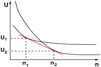
Figure 2: (Color online) Explicit Maxwell construction for determining the boundaries of phase separated regions.

The condition for the boundaries of the phase separated region is:

$$\left.\frac{dU_{1}}{dn}\right|_{n=n_{1}}=\frac{U_{2}(n_{2})-U_{1}(n_{1})}{n_{2}-n_{1}}=\left.\frac{dU_{2}}{dn}\right|_{n=n_{2}}.$$ (13)

III Results and Discussion

The internal energy of the FKLM at $T=0$ is given as an integral (2) over the product of (sub-lattice) quasi-particle density of states (QDOS) times energy up to Fermi-energy. For understanding the resulting phase-diagrams it is therefore useful to have a closer look at the QDOS first. In Fig.3 the sub-lattice MF-QDOS is shown for the different magnetic phases investigated (in 3D). The underlying full lattice is of simple cubic type with nearest neighbor hopping $T$ chosen such that the bandwidth $W$ is equal to $W=1$ eV in the case of free electrons ($J=0$ eV). The local magnetic moment is equal to $S=\frac{3}{2}$.

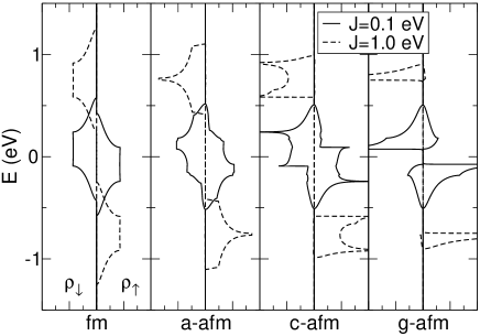
Figure 3: Sub-lattice quasi particle density of states (QDOS) of up and down electrons obtained from the MF-GF (II.2) for two values of local coupling $J$ shown for different magnetic configurations. Parameters: $S=\frac{3}{2}$ and free electron bandwidth: $W=1.0$ eV.

We have plotted the up and down-electron spectrum separately for two different values of $J=0.1/1.0$ eV. The exchange splitting $\Delta_{ex}=JS$ eV of up and down-band is clearly visible. The decisive difference between the phases for nonzero values of $J$ is bandwidth reduction from ferromagnetic over a, c to g-afm phase. The reason for this behavior becomes clear by looking at the magnetic lattices shown in Fig.1. In the ferromagnetic case an (up-)electron can move freely in all 3 directions of space without paying any additional potential energy. In a-type anti-ferromagnetic phase the electron can still move freely within a plane but when moving in the direction perpendicular to the plane it needs to overcome an energy-barrier $\Delta_{ex}$. Hence the QDOS for large values of $J$ resembles the form of 2D tight-binding dispersion. The bandwidth is reduced due to the confinement of the electrons. In the c-afm phase the electron can only move freely along one direction and the QDOS becomes effectively one dimensional. Finally in the g-type phase the electron in the large $J$ limit is quasi localized and the bandwidth gets very small. We will see soon that this bandwidth-effect is mainly responsible for the structure of the phase-diagram. Before we come to this point we want to discuss the influence of spin-flip processes as incorporated in (12).

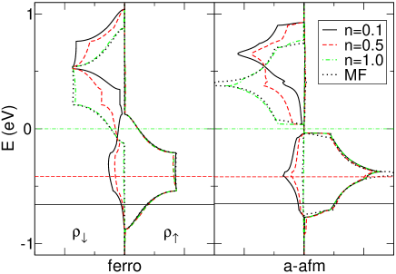
Figure 4: (Color online) Sub-lattice QDOS of up and down electrons obtained from the SF-GF (12) for three different band-fillings $n$ shown for the ferromagnetic and a-afm phase. The local coupling $J=0.5$ eV is fixed. Dotted line: corresponding MF result. Horizontal lines: respective Fermi levels. Other parameters as in Fig.3.

In Fig.4 the QDOS for $J=0.5$ eV is shown for three different band fillings $n$. The corresponding Fermi energies are marked by horizontal lines. The apparent new feature are the scattering states in the down spectrum for band fillings below half filling. Thereby the spectral weight of the scattering states is more and more reduced with increasing Fermi level. A second effect is that the sharp features in the MF-QDOS of the anti-ferromagnetic phases are smeared out. Compared to the MF results the overall change of QDOS below Fermi energy due to the inclusion of spin-flip processes is small and will not affect the form of the phase-diagram drastically. However non-negligible changes can be expected. Note that the model shows perfect particle-hole symmetry. Therefore the results for the internal energy will be the same for $n=x$ and $n=2-x$ ($x=0\dots 1$, $n=1$: half filling).
We come now to the discussion of the phase-diagrams which we got by comparing the internal energies of the different phases explicitly.

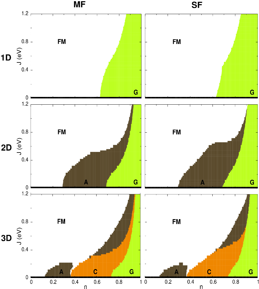
Figure 5: (Color online) First column: Phase-diagram as function of band-filling $n$ and local coupling $J$ obtained with mean-field (MF) theory (II.2) in one, two and three dimensions. Second column: Phase-diagram obtained by inclusion of spin-flip processes (SF) (12). Regions of different colors mark different (magnetic) phases: ferromagnetic (white), a-afm (brown), c-afm (orange), g-afm (green) and paramagnetic phase (black).

The pure phase-diagrams (without phase-separation) are shown in Fig.5 whereas the different phases are marked by color code. In the first column the results of the MF-calculation are shown for the 1-, 2- and 3-dimensional case. The second column shows the effects of inclusion of spin-flip processes. We will concentrate here mainly onto the 3D case since most of the given arguments hold equally for the 1D and 2D case. For $J=0$ the system is paramagnetic (black bar at bottom). For larger $J$ ($J>0$) a typical sequence appear: for low band-fillings $n$ the system is always ferromagnetic and, with increasing $n$, it becomes a-type then c-type and finally g-type anti-ferromagnetic. This behavior is understood easily by looking at the formula for the internal energy (2) and the MF-QDOS in Fig.3. Because of the bandwidth-effect discussed already the band-edge of the ferromagnetic state is always lowest in energy and will give therefore the lowest internal energy for small band-occupation. But since the QDOS of the anti-ferromagnetic phases increase much more rapidly than the ferromagnetic one, these give more weight to low energies in the integral (2) and will become lowest in energy eventually for larger band-fillings. Therefore the bandwidth-effect is main effect explaining the order of phases with increasing $n$. A very interesting feature can be found in the region: $J=0.2\dots 0.3$. In this region the ferromagnetic phase is directly followed by the c-afm phase for increasing $n$ although the a-afm phase has a larger bandwidth than the c-afm phase. This can be explained by the two-peak structure of the c-afm-QDOS. Due to the first peak at low energies these energies are much more weighted than in the a-afm case and the c-afm phase will become lower in energy than the a-afm phase. Since the reduction of bandwidth of the anti-ferromagnetic phases compared to the ferromagnetic phase is more pronounced for larger values of $J$ the ferromagnetic region is growing in this direction.
The paramagnetic phase (black bar at $J=0$) disappear for any finite $J$ since due to the down-shift of the up-spectrum of the ferromagnetic phase their internal energy will always be lower.

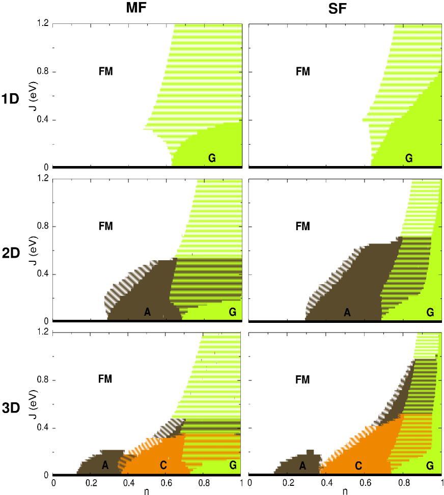
Figure 6: (Color online) Phase-diagram with phase-separation. Regions of phase-separation are marked with two-colored stripes. Color code as in Fig.5.

When comparing the MF and the SF-phase-diagram they appear to be very similar at first glance. However two interesting differences can be found, namely an increased $J$ region without a-afm-phase and the vanishing c-phase above $J\approx 0.8$eV.

Fig.6 shows the phase-diagrams where regions of phase-separation, which we have determined by an explicit Maxwell construction (13), are marked by colored stripes. The two colors denote the involved pure phases. As one can see large regions become phase-separated, whereas the two participating phases are mostly determined by the adjacent pure phases. There is one interesting exception from this: above a certain $J$ only fm/g-afm phase-separation survives and suppresses all other phases in this area. Inclusion of spin-flip processes as shown in the right column of Fig.6 push this $J$ up to higher values. Generally spin-flip processes seem to reduce phase-separation as can be seen in the g-afm phase and e.g. at the border between fm and c-afm phase.

Our results are in good qualitative agreement with numerical and DMFT results reported by othersDagotto et al. (1998); Chattopadhyay et al. (2001); Lin and Millis (2005). It is common to all these works that for small coupling strength $J$ there is only a small ferromagnetic region at low band occupation $n$ followed by more complicated (anti-ferromagnetic, spiral, canted) spin states/phase-separation. With increasing $J$ the region of fm is also increased to larger $n$ values. Near half-filling ($n=1$) one will find always anti-ferromagnetism/phase-separation. phase-diagram very similar to our 2D-FM result shown in Fig.6 was obtained by Pekker et.al.[Pekker et al., 2005]. The positions of A and G phase are in nearly perfect agreement. However the authors seem not to have taken into account phase-separation between A and G phase and their finding of FM/A phase-separation near half-filling at larger $J$ is not in accordance with our results.

IV Summary and Outlook

We have constructed phase diagrams of the FKLM in 1D, 2D and 3D by comparing the internal energies of all possible bipartite magnetic configurations of the simple cubic lattice. To this end the electronic GF is calculated by an EQM approach. We can show, that it is possible to treat all appearing higher local correlation functions exact and we derive an explicit formula for the electronic GF (12). The obtained sequence of phases with increasing band occupation $n$ and Hunds coupling $J$ is explained by the reduction of QDOS bandwidth due to electron confinement. Region of phase separation are then determined from the internal energy curves by an explicit Maxwell construction.

In the phase diagram obtained only phases appear that have explicitly considered by us. Therefore an important extension of this work could be the inclusion of more complicated spin structures like canted/spiral spin states as reported by others [Pekker et al., 2005; Garcia et al., 2004]. However the bandwidth criterion obtained here can certainly be applied to such more complicated states also.

Appendix A EQM of the Ising-GF

$$\sum_{l\mu}\left(E\delta^{\gamma\mu}_{kl}-T^{\gamma\mu}_{kl}\right)I^{\alpha\mu\beta}_{ilj\sigma}=z_{\sigma}\delta^{\gamma\beta}_{kj}\langle S^{z}_{i\alpha}\rangle$$ (14)

$$-\frac{J}{2}\left(\langle\!\langle S^{z}_{i\alpha}S^{z}_{k\gamma}c_{k\gamma\sigma};c^{+}_{j\beta\sigma}\rangle\!\rangle+z_{\sigma}\langle\!\langle S^{z}_{i\alpha}S^{-\sigma}_{k\gamma}c_{k\gamma-\sigma};c^{+}_{j\beta\sigma}\rangle\!\rangle\right.$$

$$\left.+z_{\sigma}\sum_{\sigma^{\prime}}z_{\sigma^{\prime}}\langle\!\langle S^{\sigma^{\prime}}_{i\alpha}c^{+}_{i\alpha-\sigma^{\prime}}c_{i\alpha\sigma^{\prime}}c_{k\gamma\sigma};c^{+}_{j\beta\sigma}\rangle\!\rangle\right),$$

Appendix B higher order Ising-GF

The higher order Ising-GF can be decomposed into:

$$\langle\!\langle S^{z}_{i\sigma}n_{i\alpha-\sigma}c_{i\alpha\sigma};c^{+}_{j\beta\sigma}\rangle\!\rangle\rightarrow z_{\alpha}S\langle\!\langle n_{i\alpha-\sigma}c_{i\alpha\sigma};c^{+}_{j\beta\sigma}\rangle\!\rangle$$ (15)

when a saturated sub-lattice magnetization is assumed. The EQM of the remaining GF turns out to be:

$$(E+z_{\sigma}z_{\alpha}\frac{J}{2}S)\langle\!\langle n_{i\alpha-\sigma}c_{i\alpha\sigma};c^{+}_{j\beta\sigma}\rangle\!\rangle$$

$$= \sum_{l\gamma}T^{\alpha\gamma}_{il}\langle\!\langle c^{+}_{l\gamma-\sigma}c_{i\alpha-\sigma}c_{i\alpha\sigma};c^{+}_{j\beta\sigma}\rangle\!\rangle (\mathrm{I})$$

$$+ \sum_{l\gamma}T^{\alpha\gamma}_{il}\langle\!\langle c^{+}_{i\alpha-\sigma}c_{l\gamma-\sigma}c_{i\alpha\sigma};c^{+}_{j\beta\sigma}\rangle\!\rangle (\mathrm{II})$$

$$+ \sum_{l\gamma}T^{\alpha\gamma}_{il}\langle\!\langle c^{+}_{i\alpha-\sigma}c_{i\alpha-\sigma}c_{l\gamma\sigma};c^{+}_{j\beta\sigma}\rangle\!\rangle (\mathrm{III})$$

$$- 2\sum_{l\gamma}T^{\alpha\gamma}_{il}\langle\!\langle c^{+}_{l\gamma-\sigma}c_{i\alpha-\sigma}c_{i\alpha\sigma};c^{+}_{j\beta\sigma}\rangle\!\rangle$$

$$+ \delta^{\alpha\beta}_{ij}\langle n_{i\alpha-\sigma}\rangle-\frac{J}{2}\langle\!\langle S^{-\sigma}_{i\alpha}n_{i\alpha\sigma}c_{i\alpha-\sigma};c^{+}_{j\beta\sigma}\rangle\!\rangle.$$ (16)

Subtracting the term denoted by (I) from this equation one gets:

$$\sum_{l\gamma}(E\delta^{\alpha\gamma}_{il}-T^{\alpha\gamma}_{il}+z_{\sigma}z_{\alpha}\delta^{\alpha\gamma}_{il}\frac{J}{2}S)\times$$ (17)

$$\langle\!\langle c^{+}_{l\gamma-\sigma}c_{i\alpha-\sigma}c_{i\alpha\sigma};c^{+}_{j\beta\sigma}\rangle\!\rangle$$

$$= \sum_{l\gamma}T^{\alpha\gamma}_{il}\langle\!\langle c^{+}_{i\alpha-\sigma}c_{l\gamma-\sigma}c_{i\alpha\sigma};c^{+}_{j\beta\sigma}\rangle\!\rangle$$

$$+ \sum_{l\gamma}T^{\alpha\gamma}_{il}\langle\!\langle c^{+}_{i\alpha-\sigma}c_{i\alpha-\sigma}c_{l\gamma\sigma};c^{+}_{j\beta\sigma}\rangle\!\rangle$$

$$- 2\sum_{l\gamma}T^{\alpha\gamma}_{il}\langle\!\langle c^{+}_{l\gamma-\sigma}c_{i\alpha-\sigma}c_{i\alpha\sigma};c^{+}_{j\beta\sigma}\rangle\!\rangle$$

$$+ \delta^{\alpha\beta}_{ij}\langle n_{i\alpha-\sigma}\rangle-\frac{J}{2}\langle\!\langle S^{-\sigma}_{i\alpha}n_{i\alpha\sigma}c_{i\alpha-\sigma};c^{+}_{j\beta\sigma}\rangle\!\rangle.$$

This can be solved for $\langle\!\langle n_{i\alpha-\sigma}c_{i\alpha\sigma};c^{+}_{j\beta\sigma}\rangle\!\rangle$ by left-multiplying with the MF-GF matrix:

$$\langle\!\langle n_{i\alpha-\sigma}c_{i\alpha\sigma};c^{+}_{i\alpha\sigma}\rangle\!\rangle=$$ (18)

$$\sum_{kl\eta\gamma}G^{(\mathrm{MF})\alpha\eta}_{ik\sigma}T^{\eta\gamma}_{kl}\langle\!\langle c^{+}_{i\alpha-\sigma}c_{l\gamma-\sigma}c_{i\alpha\sigma};c^{+}_{j\beta\sigma}\rangle\!\rangle$$

$$+ \sum_{kl\eta\gamma}G^{(\mathrm{MF})\alpha\eta}_{ik\sigma}T^{\eta\gamma}_{kl}\langle\!\langle c^{+}_{i\alpha-\sigma}c_{i\alpha-\sigma}c_{l\gamma\sigma};c^{+}_{j\beta\sigma}\rangle\!\rangle$$

$$- 2\sum_{kl\eta\gamma}G^{(\mathrm{MF})\alpha\eta}_{ik\sigma}T^{\eta\gamma}_{kl}\langle\!\langle c^{+}_{l\gamma-\sigma}c_{i\alpha-\sigma}c_{i\alpha\sigma};c^{+}_{j\beta\sigma}\rangle\!\rangle$$

$$+ G^{(\mathrm{MF})\alpha\beta}_{ij\sigma}\langle n_{j\beta-\sigma}\rangle$$

$$- \frac{J}{2}\sum_{k\eta}G^{(\mathrm{MF})\alpha\eta}_{ik\sigma}\langle\!\langle S^{-\sigma}_{k\eta}n_{k\eta\sigma}c_{k\eta-\sigma};c^{+}_{j\beta\sigma}\rangle\!\rangle.$$

Two other equations are obtained from (B) by subtracting term (II) or (III) and performing the same steps as before. This yields:

$$\langle\!\langle n_{i\alpha-\sigma}c_{i\alpha\sigma};c^{+}_{i\alpha\sigma}\rangle\!\rangle=$$ (19)

$$\sum_{kl\eta\gamma}G^{(\mathrm{MF})\alpha\eta}_{ik\sigma}T^{\eta\gamma}_{kl}\langle\!\langle c^{+}_{l\gamma-\sigma}c_{i\alpha-\sigma}c_{i\alpha\sigma};c^{+}_{j\beta\sigma}\rangle\!\rangle$$

$$+ \sum_{kl\eta\gamma}G^{(\mathrm{MF})\alpha\eta}_{ik\sigma}T^{\eta\gamma}_{kl}\langle\!\langle c^{+}_{i\alpha-\sigma}c_{i\alpha-\sigma}c_{l\gamma\sigma};c^{+}_{j\beta\sigma}\rangle\!\rangle$$

$$- 2\sum_{kl\eta\gamma}G^{(\mathrm{MF})\alpha\eta}_{ik\sigma}T^{\eta\gamma}_{kl}\langle\!\langle c^{+}_{l\gamma-\sigma}c_{i\alpha-\sigma}c_{i\alpha\sigma};c^{+}_{j\beta\sigma}\rangle\!\rangle$$

$$+ G^{(\mathrm{MF})\alpha\beta}_{ij\sigma}\langle n_{j\beta-\sigma}\rangle$$

$$- \frac{J}{2}\sum_{k\eta}G^{(\mathrm{MF})\alpha\eta}_{ik\sigma}\langle\!\langle S^{-\sigma}_{k\eta}n_{k\eta\sigma}c_{k\eta-\sigma};c^{+}_{j\beta\sigma}\rangle\!\rangle$$

and

$$\langle\!\langle n_{i\alpha-\sigma}c_{i\alpha\sigma};c^{+}_{i\alpha\sigma}\rangle\!\rangle=$$ (20)

$$\sum_{kl\eta\gamma}G^{(\mathrm{MF})\alpha\eta}_{ik\sigma}T^{\eta\gamma}_{kl}\langle\!\langle c^{+}_{l\gamma-\sigma}c_{i\alpha-\sigma}c_{i\alpha\sigma};c^{+}_{j\beta\sigma}\rangle\!\rangle$$

$$+ \sum_{kl\eta\gamma}G^{(\mathrm{MF})\alpha\eta}_{ik\sigma}T^{\eta\gamma}_{kl}\langle\!\langle c^{+}_{i\alpha-\sigma}c_{l\gamma-\sigma}c_{i\alpha\sigma};c^{+}_{j\beta\sigma}\rangle\!\rangle$$

$$- 2\sum_{kl\eta\gamma}G^{(\mathrm{MF})\alpha\eta}_{ik\sigma}T^{\eta\gamma}_{kl}\langle\!\langle c^{+}_{l\gamma-\sigma}c_{i\alpha-\sigma}c_{i\alpha\sigma};c^{+}_{j\beta\sigma}\rangle\!\rangle$$

$$+ G^{(\mathrm{MF})\alpha\beta}_{ij\sigma}\langle n_{j\beta-\sigma}\rangle$$

$$- \frac{J}{2}\sum_{k\eta}G^{(\mathrm{MF})\alpha\eta}_{ik\sigma}\langle\!\langle S^{-\sigma}_{k\eta}n_{k\eta\sigma}c_{k\eta-\sigma};c^{+}_{j\beta\sigma}\rangle\!\rangle$$

Adding (19) and (20) and subtracting (18) one finally gets:

$$\langle\!\langle S^{z}_{i\alpha}n_{i\alpha-\sigma}c_{i\alpha\sigma};c^{+}_{j\beta\sigma}\rangle\!\rangle=z_{\alpha}S\left(G^{\alpha\beta(\mathrm{MF})}_{ij\sigma}\langle n_{j\beta-\sigma}\rangle\right.$$ (21)

$$\left.-\frac{J}{2}\sum_{l\gamma}G^{\alpha\gamma(\mathrm{MF})}_{il\sigma}\langle\!\langle S^{-\sigma}_{l\gamma}n_{l\gamma\sigma}c_{l\gamma-\sigma};c^{+}_{j\beta\sigma}\rangle\!\rangle\right).$$

References

- Zener (1951a) C. Zener, Phys. Rev. 81, 440 (1951a).
- Zener (1951b) C. Zener, Phys. Rev. 82, 403 (1951b).
- Dagotto (2003) E. Dagotto, Nanoscale Phase Separation and Colossal Magnetoresistance (Springer, Berlin, 2003).
- Stier and Nolting (2007) M. Stier and W. Nolting, Phys. Rev. B 75, 144409 (2007).
- Stier and Nolting (2008) M. Stier and W. Nolting, Phys. Rev. B 78, 144425 (2008).
- Busch et al. (1964) G. Busch, P. Junod, and P. Wachter, Physics Letters 12, 11 (1964).
- Rys et al. (1967) F. Rys, J. S. Helman, and W. Baltensperger, Physik der Kondensierten Materie, Volume 6, Issue 2, pp.105-125 6, 105 (1967).
- Santos et al. (2004) C. Santos, W. Nolting, and V. Eyert, Phys. Rev. B 69, 214412 (2004).
- Yunoki et al. (1998) S. Yunoki, J. Hu, A. L. Malvezzi, A. Moreo, N. Furukawa, and E. Dagotto, Phys. Rev. Lett. 80, 845 (1998).
- Kagan et al. (1999) M. Y. Kagan, D. I. Khomskii, and M. V. Mostovoy, European Physical Journal B 12, 217 (1999), eprint arXiv:cond-mat/9804213.
- Chattopadhyay et al. (2001) A. Chattopadhyay, A. J. Millis, and S. Das Sarma, Phys. Rev. B 64, 012416 (2001), eprint arXiv:cond-mat/0004151.
- Lin and Millis (2005) C. Lin and A. J. Millis, Phys. Rev. B 72, 245112 (2005), eprint arXiv:cond-mat/0509004.
- Pekker et al. (2005) D. Pekker, S. Mukhopadhyay, N. Trivedi, and P. M. Goldbart, Phys. Rev. B 72, 075118 (2005).
- Dagotto et al. (1998) E. Dagotto, S. Yunoki, A. L. Malvezzi, A. Moreo, J. Hu, S. Capponi, D. Poilblanc, and N. Furukawa, Phys. Rev. B 58, 6414 (1998).
- Garcia et al. (2004) D. J. Garcia, K. Hallberg, B. Alascio, and M. Avignon, Phys. Rev. Lett. 93, 177204 (2004).
- Kienert and Nolting (2006) J. Kienert and W. Nolting, Phys. Rev. B 73, 224405 (2006), eprint arXiv:cond-mat/0606485.
- Peters and Pruschke (2007) R. Peters and T. Pruschke, Phys. Rev. B 76, 245101 (2007), eprint 0707.0277.
- Georges et al. (1996) A. Georges, G. Kotliar, W. Krauth, and M. J. Rozenberg, Rev. Mod. Phys. 68, 13 (1996).
- Nolting et al. (1997) W. Nolting, S. Rex, and S. Mathi Jaya, J. Phys.: Condens. Matter 9, 1301 (1997).
- Santos and Nolting (2002) C. Santos and W. Nolting, Phys. Rev. B 65, 144419 (2002).
- Shastry and Mattis (1981) B. S. Shastry and D. C. Mattis, Phys. Rev. B 24, 5340 (1981).
- Allan and Edwards (1982) S. R. Allan and D. M. Edwards, J. Phys. C 15, 2151 (1982).
- Nolting and Matlak (1984) W. Nolting and M. Matlak, Phys. Status Solidi B 123, 155 (1984).
- Anderson (1952) P. W. Anderson, Phys. Rev. 86, 694 (1952).