Progress on Calorons

Abstract:

The progress on calorons (finite temperature instantons) is sketched. In particular there is some interest for confining temperatures, where the holonomy is non-trivial.

1 Introduction

There has been a revised interest in studying instantons at finite temperature $T$, so-called calorons [1, 2], because new explicit solutions could be obtained where the Polyakov loop at spatial infinity (the so-called holonomy) is non-trivial. They reveal more clearly the monopole constituent nature of these calorons [3]. Non-trivial holonomy is therefore expected to play a role in the confined phase (i.e. for $T<T_{c}$) where the trace of the Polyakov loop fluctuates around small values. The properties of instantons are therefore directly coupled to the order parameter for the deconfining phase transition.

At finite temperature $A_{0}$ plays in some sense the role of a Higgs field in the adjoint representation, which explains why magnetic monopoles occur as constituents of calorons. Since $A_{0}$ is not necessarily static it is better to consider the Polyakov loop as the analog of the Higgs field, $P(t,\vec{x})={\rm Pexp}\left(\int_{0}^{\beta}A_{0}(t+s,\vec{x})ds\right)$, which transforms under a periodic gauge transformation $g(x)$ to $g(x)P(x)g^{-1}(x)$, like an adjoint Higgs field. Here $\beta=1/kT$ is the period in the imaginary time direction, under which the gauge field is assumed to be periodic. Finite action requires the Polyakov loop at spatial infinity to be constant. For SU($n$) gauge theory this gives ${{\cal P}_{\infty}}=\lim_{|\vec{x}|\to\infty}P(0,\vec{x})=g^{\dagger}\exp(2\pi i{\rm diag}(\mu_{1},\mu_{2},\ldots,\mu_{n}))g$, where $g$ brings ${{\cal P}_{\infty}}$ to its diagonal form, with $n$ eigenvalues being ordered according to $\sum_{i=1}^{n}\mu_{i}=0$ and $\mu_{1}\leq\mu_{2}\leq\ldots\leq\mu_{n}\leq\mu_{n+1}\equiv 1+\mu_{1}$. In the algebraic gauge, where $A_{0}(x)$ is transformed to zero at spatial infinity, the gauge fields satisfy the boundary condition $A_{\mu}(t+\beta,\vec{x})={{\cal P}_{\infty}}A_{\mu}(t,\vec{x}){\cal{P}}_{\infty}^{-1}$.

Caloron solutions are such that the total magnetic charge vanishes. A single caloron with topological charge one contains $n-1$ monopoles with a unit magnetic charge in the $i$-th U(1) subgroup, which are compensated by the $n$-th monopole of so-called type $(1,1,\ldots,1)$, having a magnetic charge in each of these subgroups [4]. At topological charge $k$ there are $kn$ constituents, $k$ monopoles of each of the $n$ types. Monopoles of type $j$ have a mass $8\pi^{2}\nu_{j}/\beta$, with $\nu_{j}\equiv\mu_{j+1}-\mu_{j}$. The sum rule $\sum_{j=1}^{n}\!\nu_{j}\!=\!1$ guarantees the correct action, $8\pi^{2}k$.

Prior to their explicit construction, calorons with non-trivial holonomy were considered irrelevant [2], because the one-loop correction gives rise to an infinite action barrier. However, the infinity simply arises due to the integration over the finite energy density induced by the perturbative fluctuations in the background of a non-trivial Polyakov loop [5]. The calculation of the non-perturbative contribution was performed in [6]. When added to this perturbative contribution, with minima at center elements, these minima turn unstable for decreasing temperature right around the expected value of $T_{c}$. This lends some support to monopole constituents being the relevant degrees of freedom which drive the transition from a phase in which the center symmetry is broken at high temperatures to one in which the center symmetry is restored at low temperatures. Lattice studies, both using cooling [7] and chiral fermion zero-modes [8] as filters, have also conclusively confirmed that monopole constituents do dynamically occur in the confined phase.

2 Some Properties of Caloron Solutions

Using the classical scale invariance we can always arrange $\beta=1$, as will be assumed throughout. A remarkably simple formula for the $SU(n)$ action density exists [4],

$${\rm Tr}F_{\alpha\beta}^{\,2}(x)=\partial_{\alpha}^{2}\partial_{\beta}^{2}\log\psi(x),\quad\psi(x)={\scriptstyle{\frac{1}{2}}}{\rm tr}({\cal{A}}_{n}\cdots{\cal{A}}_{1})-\cos(2\pi t),$$

$${\cal{A}}_{m}\equiv\frac{1}{r_{m}}\left(\!\!\!\begin{array}[]{cc}r_{m}\!\!&|\vec{\rho}_{m+1}|\\ 0\!\!&r_{m+1}\end{array}\!\!\!\right)\left(\!\!\!\begin{array}[]{cc}\cosh(2\pi\nu_{m}r_{m})\!\!&\sinh(2\pi\nu_{m}r_{m})\\ \sinh(2\pi\nu_{m}r_{m})\!\!&\cosh(2\pi\nu_{m}r_{m})\end{array}\!\!\!\right),$$ (5)

with $r_{m}\equiv|\vec{x}-\vec{y}_{m}|$ and $\vec{\rho}_{m}\equiv\vec{y}_{m}-\vec{y}_{m-1}$, where $\vec{y}_{m}$ is the location of the $m^{\rm th}$ constituent monopole with a mass $8\pi^{2}\nu_{m}$. Note that the index $m$ should be considered mod $n$, such that e.g. $r_{n+1}=r_{1}$ and $\vec{y}_{n+1}=\vec{y}_{1}$ (there is one exception, $\mu_{n+1}=1+\mu_{1}$). It is sufficient that only one constituent location is far separated from the others, to show that one can neglect the $\cos(2\pi t)$ term in $\psi(x)$, giving rise to a static action density in this limit [4].

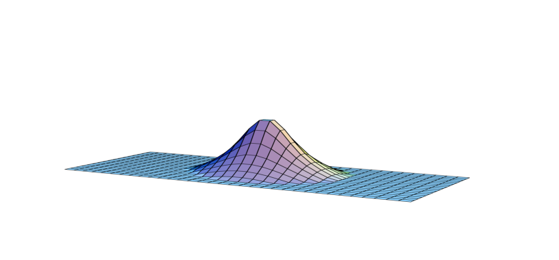
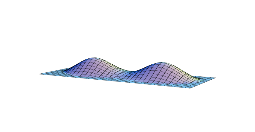
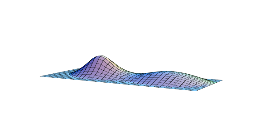
Figure 1: Shown are three charge one SU(2) caloron profiles at $t=0$ with $\beta=1$ and $\rho=1$. From left to right for $\mu_{2}=-\mu_{1}=0$ ($\nu_{1}=0,\nu_{2}=1$), $\mu_{2}=-\mu_{1}=0.125$ ($\nu_{1}=1/4,\nu_{2}=3/4$) and $\mu_{2}=-\mu_{1}=0.25$ ($\nu_{1}=\nu_{2}=1/2$) on equal logarithmic scales, cutoff below an action density of $1/(2e)$.

In Fig. 1 we show how for SU(2) there are two lumps, except that the second lump is absent for trivial holonomy. Fig. 2 demonstrates for SU(2) and SU(3) that there are indeed $n$ lumps (for SU($n$)) which can be put anywhere. These lumps are constituent monopoles, where one of them has a winding in the temporal direction (which cannot be seen from the action density).

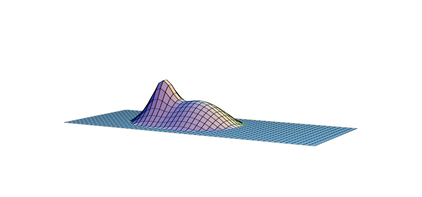
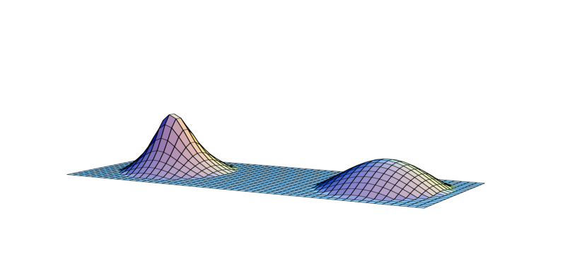
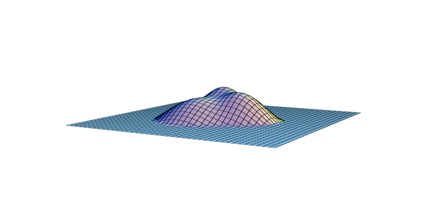
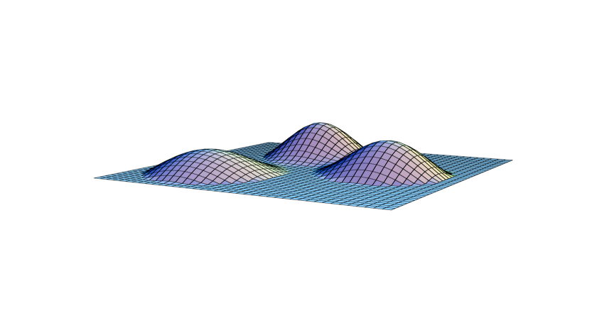
Figure 2: On the left are shown two charge one SU(2) caloron profiles at $t=0$ with $\beta=1$ and $\mu_{2}=-\mu_{1}=0.125$, for $\rho=1.6$ (bottom) and 0.8 (top) on equal logarithmic scales, cutoff below an action density of $1/(2e^{2})$. On the right are shown two charge one SU(3) caloron profiles at $t=0$ and $(\nu_{1},\nu_{2},\nu_{3})=(1/4,7/20,2/5)$, implemented by $(\mu_{1},\mu_{2},\mu_{3})=(-17/60,-1/30,19/60)$. The bottom configuration has the location of the lumps scaled by $8/3$. They are cutoff at $1/(2e)$.

2.1 Fermion Zero-Modes

An essential property of calorons is that the chiral fermion zero-modes are localized to constituents of a certain charge only. The latter depends on the choice of boundary condition for the fermions in the imaginary time direction (allowing for an arbitrary U(1) phase $\exp(2\pi iz)$) [9]. This provides an important signature for the dynamical lattice studies, using chiral fermion zero-modes as a filter [8]. To be precise, the zero-modes are localized to the monopoles of type $m$ provided $\mu_{m}<z<\mu_{m+1}$. Denoting the zero-modes by $\hat{\Psi}_{z}(x)$, we can write $\hat{\Psi}^{\dagger}_{z}(x)\hat{\Psi}_{z}(x)=-(2\pi)^{-2}\partial_{\mu}^{2}\hat{f}_{x}(z,z)$, where $\hat{f}_{x}(z,z^{\prime})$ is a Green’s function which for $z\in[\mu_{m},\mu_{m+1}]$ satisfies $\hat{f}_{z}(z,z)=\pi<\!\!v_{m}(z)|{\cal{A}}_{m\!-\!1}\cdots{\cal{A}}_{1}{\cal{A}}_{n}\cdots{\cal{A}}_{m}|w_{m}(z)\!\!>/(r_{m}\psi)$, where the spinors $v_{m}$ and $w_{m}$ are defined by $v_{m}^{1}(z)=-w_{m}^{2}(z)=\sinh\left(2\pi(z\!-\!\mu_{m})r_{m}\right)$, and $v_{m}^{2}(z)=w_{m}^{1}(z)=\cosh\left(2\pi(z\!-\!\mu_{m})r_{m}\right)$.

To obtain the finite temperature fermion zero-mode one puts $z={\scriptstyle{\frac{1}{2}}}$, whereas for the fermion zero-mode with periodic boundary conditions one takes $z=0$. From this it is easily seen that in case of well separated constituents the zero-mode is localized only at $\vec{y}_{m}$ for which $z\in[\mu_{m},\mu_{m+1}]$. To be specific, in this limit $\hat{f}_{x}(z,z)=\pi\tanh(\pi r_{m}\nu_{m})/r_{m}$ for $SU(2)$, and more generally $\hat{f}_{x}(z,z)=2\pi\sinh[2\pi(z-\mu_{m})r_{m}]\sinh[2\pi(\mu_{m+1}-z)r_{m}]/(r_{m}\sinh[2\pi\nu_{m}r_{m}])^{-1}$. We illustrate in Fig. 3 the localization of the fermion zero-modes for the case of $SU(3)$.

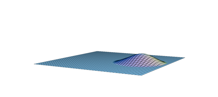
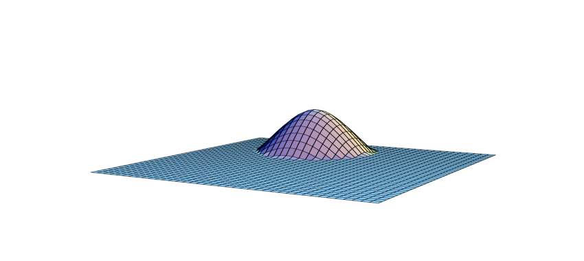
Figure 3: For the SU(3) configuration in the lower right corner of Fig. 2 we have determined on the left the zero-mode density for fermions with anti-periodic boundary conditions in time and on the right for periodic boundary conditions. They are plotted at equal logarithmic scales, cut off below $1/e^{5}$.

2.2 Calorons of Higher Charge

We have been able to use a “mix” of the ADHM and Nahm formalism [10], both in making powerful approximations, like in the far field limit (based on our ability to identify the exponentially rising and falling terms), and for

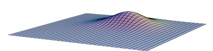
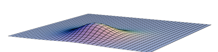
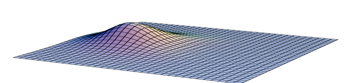
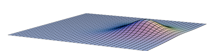
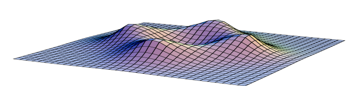
Figure 4: In the middle is shown the action density in the plane of the constituents at $t=0$ for an SU(2) charge 2 caloron with ${\rm tr}\,{{\cal P}_{\infty}}=0$, where all constituents strongly overlap. On a scale enhanced by a factor $10\pi^{2}$ are shown the densities for the two zero-modes, using either periodic (left) or anti-periodic (right) boundary conditions in the time direction.

finding exact solutions through solving the homogeneous Green’s function [11]. We found axially symmetric solutions for arbitrary $k$, as well as for $k=2$ two sets of non-trivial solutions for the matching conditions that interpolate between overlapping and well-separated constituents. For this task we could make use of an existing analytic result for charge-2 monopoles [12], adapting it to the case of carolons. An example is shown in Fig. 4.

There has also been some progress on constructing the hyperKähler metric which approximates the metric for an arbitrary number of calorons. They claim that this already gives confinement [13]. For the implications of caloron constituents near the phase transition see [14].

References

- [1] B.J. Harrington and H.K. Shepard, Phys. Rev. D17 (1978) 2122; Phys. Rev. D18 (1978) 2990.
- [2] D.J. Gross, R.D. Pisarski and L.G. Yaffe, Rev. Mod. Phys. 53 (1981) 43.
- [3] T.C. Kraan and P. van Baal, Phys. Lett. B428 (1998) 268 [hep-th/9802049]; Nucl. Phys. B533 (1998) 627 [hep-th/9805168]; K. Lee, Phys. Lett B426 (1998) 323 [hep-th/9802012]; K. Lee and C. Lu, Phys. Rev. D58 (1998) 025011 [hep-th/9802108].
- [4] T.C. Kraan and P. van Baal, Phys. Lett. B435 (1998) 389 [hep-th/9806034].
- [5] N. Weiss, Phys. Rev. D24 (1981) 475.
- [6] D. Diakonov, N. Gromov, V. Petrov and S. Slizovskiy, Phys. Rev. D70 (2004) 036003 [hep-th/0404042]; D. Diakonov and N. Gromov, Phys. Rev. D72 (2005) 025003 [hep-th/0502132].
- [7] E.-M. Ilgenfritz, B.V. Martemyanov, M. Müller-Preussker, S. Shcheredin and A.I. Veselov, Phys. Rev. D66 (2002) 074503 [hep-lat/0206004]; F. Bruckmann, E.-M. Ilgenfritz, B.V. Martemyanov and P. van Baal, Phys. Rev. D70 (2004) 105013 [hep-lat/0408004]; P. Gerhold, E.-M. Ilgenfritz and M. Müller-Preussker, Nucl. Phys. B760 (2007) 1 [hep-ph/0607315].
- [8] C. Gattringer and S. Schaefer, Nucl. Phys. B654 (2003) 30 [hep-lat/0212029]; C. Gattringer and R. Pullirsch, Phys.Rev. D69 (2004) 094510 [hep-lat/0402008].
- [9] M. García Pérez, A. González-Arroyo, C. Pena and P. van Baal, Phys. Rev. D60 (1999) 031901 [hep-th/9905016]; M.N. Chernodub, T.C. Kraan and P. van Baal, Nucl. Phys. B(Proc.Suppl.)83-84 (2000) 556.
- [10] M.F. Atiyah, N.J. Hitchin, V. Drinfeld and Yu.I. Manin, Phys. Lett. 65A (1978) 185; W. Nahm, “Self-dual monopoles and calorons,” in: Lecture Notes in Physics, 201 (1984) 189.
- [11] F. Bruckmann and P. van Baal, Nucl. Phys. B645 (2002) 105 [hep-th/0209010]; F. Bruckmann, D. Nógrádi and P. van Baal, Nucl. Phys. B666 (2003) 197 [hep-th/0305063]; Nucl. Phys. B698 (2004) 233 [hep-th/0404210].
- [12] H. Panagopoulos, Phys. Rev. D28 (1983) 380.
-
[13]
D. Diakonov and V. Petrov, Phys. Rev. D76 (2007) 056001
[arXiv:0704.3181 [hep-th]];
D. Diakonov, Acta Phys. Polon. B39 (2008) 3365 [arXiv:0807.0902 [hep-th]]; D. Diakonov and V. Petrov, “Statistical physics of dyons and quark confinement,” arXiv:0809.2063 [hep-th]. - [14] F. Bruckmann, “How instantons could survive the phase transition,” arXiv:0901.0987 [hep-ph].