Qubit Coherent Control with Squeezed Light Fields

Abstract

We study the use of squeezed light for qubit coherent control and compare it with the coherent state control field case. We calculate the entanglement between a short pulse of resonant squeezed light and a two-level atom in free space and the resulting operation error. We find that the squeezing phase, the phase of the light field and the atomic superposition phase, all determine whether atom-pulse mode entanglement and the gate error are enhanced or suppressed. However, when averaged over all possible qubit initial states, the gate error would not decrease by a practicably useful amount and would in fact increase in most cases. We discuss the possibility of measuring the increased gate error as a signature of the enhancement of entanglement by squeezing.

I Introduction

The coherent control of a two-level atom in free space with resonant laser fields is important both from a fundamental as well as a practical standpoint. In particular, for quantum information processing purposes, where the two-level atom encodes a single quantum bit (qubit), coherent control accuracy plays a crucial role. Fault-tolerant quantum error correction schemes, necessary for large scale quantum computing, demand that the error in a single quantum gate is below a certain, typically very small, threshold Knill 2005 .

In recent years the fundamental limitation to qubit control accuracy imposed by the quantum nature of the control light fields has been the focus of several studies VE-K ; banacloche ; SD-PRA68 ; itano ; SD-PRA69 ; Nha-Carmichael . For a coherent state of light (CL), where both phase and amplitude fluctuations are at the standard quantum limit (SQL), it was found that the gate error is determined by the qubit spontaneous decay rate. At a time shorter than the qubit decay time, part of that error can be interpreted as due to entanglement between the control field mode and the qubit (forward scattering).

This entanglement is a measure of the information on the atomic state carried away by the pulse field and could, in principle, be exploited as a resource in quantum communication schemes. For a CL pulse of duration $\tau$, the entanglement, measured by the tangle $T$, was found to be SD-PRA69 , $T\sim\tau\sim 1/\sqrt{\bar{n}}$, where $\bar{n}$ is the average number of photons in the pulse. Thus, in agreement with the correspondence principle, quantum entanglement becomes very small as the pulse approaches the classical limit, i.e. $\bar{n}\gg 1$.

It is therefore natural to ask whether a control with non coherent light field states would reduce or increase both the operation error and atom-light mode entanglement. In this paper we investigate the fundamental quantum limitation to the fidelity of qubit coherent control with squeezed light (SL) fields. As opposed to CL, SL has phase-dependent quantum fluctuations, where one field quadrature has reduced and the other increased fluctuations compared with the SQL. Reduced phase fluctuations of squeezed light have been shown to, in principle, improve the fundamental limitation to phase metrology accuracy Caves81 ; Grangier87 . The use of squeezed light states was also shown to be beneficial for continuous variable quantum key distribution Ralph ; Hillery ; Preskill . Here, we explore the possible advantage of the use of squeezed light for qubit coherent control. Both the error of a single-qubit quantum gate and the entanglement between the atomic qubit and the SL mode are calculated.

Atom-SL interactions were studied extensively in the past DF-rev ; DF-book . In most cases the atomic dynamics was found to be modified in a squeezing-phase-dependent way. Gardiner gar86 found that a two-level atom damped by a squeezed vacuum reservoir exhibits squeezing-phase-dependent suppression or enhancement of atomic coherence decay. Carmichael car87 added a coherent field that drives the atom and showed that the dynamics of the atomic coherence depends on the squeezed vacuum and the coherent driving field relative phase. Both assumed a broadband squeezed vacuum reservoir whereas the finite bandwidth case was studied in ParGar . Milburn, on the other hand, studied the interaction of a single-mode SL with an atom using the Janes-Cummings model and found a squeezing-phase-dependent increase or decrease of the collapse time Milburn_JC .

Here we assume a qubit that is encoded in an atomic, two-level, superposition and a control field that is realized with a pulse of SL in a single electromagnetic (EM) field mode and of duration shorter than the typical atomic decay time, in free space. We find that the squeezing phase, the phase of the light field and the atomic superposition phase, all determine whether atom-pulse mode entanglement and the gate error are enhanced or suppressed. It is found that, although reduced for certain qubit initial states, when averaged over all possible states the minimal gate error is comparable to that with CL fields.

The paper is outlined as follows. Section II describes a general model of the interaction between a light pulse and an atom in free space within the paraxial approximation. In Sec. III the pulse mode is assumed to be in a squeezed state and its effect on the atom is examined. Atom-pulse entanglement as well as the operation error are calculated. Some aspects of possible experimental realization are discussed in Sec. IV where our results are also briefly summarized.

II General Model and Approach

We describe the interaction of a two-level atom with a quantized pulse of light propagating in free space. Classically the propagation of such a pulse is well approximated by a paraxial wave equation. A paraxial formalism for quantized pulses was described in woerdman ; SD-PRA68 ; Deutsch . We briefly describe the paraxial model following a similar approach to that in SD-PRA68 . The derivation of this approximation is outlined in the appendix, where we start from the basic atom-field Hamiltonian in free space and get to the model described below.

II.1 The pulse mode

Consider a laser pulse traveling in the $z$ direction and interacting with a well-localized atom or ion at position $\vec{r}_{a}$. This pulse is a wave packet of Fourier modes around some wave vector $\vec{k}_{0}=k_{0}\vec{z}$, where $\vec{z}$ is a unit vector pointing to the $z$ direction, i.e. it is composed of a carrier wave vector $\vec{k}_{0}$ and a slowly varying envelope. The pulse is assumed to propagate with a small diffraction angle, so that the paraxial approximation is valid. A natural description for such a pulse is as a superposition of Gaussian beams with a well-defined transverse area $A$ at the position of the atom, each with wave number $k_{0}+k$, where $k\ll k_{0}$, analogous to a narrowband wave packet of Fourier modes in 1d. In this approximation the pulse is effectively a one-dimensional beam with transverse area $A$ similar to a Gaussian beam. The envelope of the pulse mode, $\varphi_{f_{0}}(z)$, is a function of width $c\tau$ where $\tau$ is the pulse duration and $c$ the speed of light. The field operator assigned to this pulse mode is $\hat{a}_{f_{0}}$.

II.2 Interaction picture and the atom-pulse bipartite system

We start with the full atom-field Hamiltonian in free space,

$$\hat{H}=\hat{H}_{F}+\hat{H}_{A}+\hat{H}_{AF}$$

$$\hat{H}_{A}+\hat{H}_{F}=\frac{1}{2}\ \hbar\omega_{a}\hat{\sigma}_{z}+\sum_{\vec{k}\mu}\hbar\omega_{k}\hat{a}^{\dagger}_{\vec{k}\mu}\hat{a}_{\vec{k}\mu}$$

$$\hat{H}_{AF}=\sum_{\vec{k}\mu}i\hbar\left(g_{\vec{k}\mu}\hat{a}_{\vec{k}\mu}-h.c.\right)\left(\hat{\sigma}_{+}+\hat{\sigma}_{-}\right),$$ (1)

where $\vec{k}\mu$ are the indices of a Fourier mode and its polarization respectively, and $g_{\vec{k}\mu}$ are the atom-mode couplings. Here the $\hat{\sigma}$ operators are the spin $1/2$ Pauli matrices and $\hbar\omega_{a}$ is the energy separation between the two atomic levels. Moving to the interaction picture with respect to the interaction $\hat{H}_{AF}$ in the rotating wave approximation, assuming no detuning $\omega_{0}=k_{0}c=\omega_{a}$, and using the paraxial approximation, we get the Hamiltonian in the interaction picture (see appendix)

$$\hat{H}_{I} = \hat{H}_{S}+\hat{H}_{SR}$$

$$\hat{H}_{S} = i\hbar g_{f_{0}}(t)\left(\ \hat{a}_{f_{0}}\hat{\sigma}_{+}-\hat{a}_{f_{0}}^{{\dagger}}\hat{\sigma}_{-}\right)$$

$$\hat{H}_{SR} = i\hbar\sum_{r}\left(g_{r}\hat{a}_{r}\hat{\sigma}_{+}-g_{r}^{\ast}\hat{a}_{r}^{\dagger}\hat{\sigma}_{-}\right),$$ (2)

where the indices $\{r\}$ denote all the free space EM modes apart from the $f_{0}$ pulse mode, with couplings $g_{r}$ which are in general time dependent. The $f_{0}$ mode coupling is

$$g_{f_{0}}(t)=d\sqrt{\frac{\omega_{0}}{2\epsilon_{0}\hbar A}}e^{ik_{0}z_{a}}\varphi_{f_{0}}(z_{a}-ct),$$ (3)

where $z_{a}$ is the atom’s position. In Eq. (2) we assume both the envelope of the pulse $\varphi_{f_{0}}(z)$ and the dipole matrix element $d$ to be real and set $z_{a}=0$. A similar model Hamiltonian was also used in SD-PRA69 ; VE-K where the entanglement between a CL pulse and an atom was calculated. Note that the time dependence of the atom-pulse coupling $g_{f_{0}}(t)$ is identical to that of the pulse, the pulse therefore switches the interaction on and off.

The relevant bipartite system is composed of the atom and the $f_{0}$ light mode, coupled by $\hat{H}_{S}$. The rest of the EM modes except for $f_{0}$, $\{r\}$, make up a reservoir that interacts with the bipartite system via the coupling with the atom.

III Squeezed Light Pulse operating on an atom

We consider a pulse of squeezed light operating on an atom. The pulse’s average field changes the atomic superposition coherently. In a Bloch sphere representation this corresponds to a rotation of the Bloch vector. The quantum fluctuations of the field lead to atom-pulse entanglement and add a random component to the average operation. We wish to analyze and calculate the error caused by quantum fluctuations as well as the degree of atom-pulse mode entanglement. The model outlined in Sec. II is sufficiently general to describe a pulse in any quantum state and its interaction with the atom. In SD-PRA69 ; VE-K calculations for CL state were performed. In this Section we will discuss quantum pulses of SL interacting with a two-level atom. The general formalism is presented in Sec. III A. In Sec. III B we consider a rotation of the Bloch vector by 180 degrees about an axis lying in the Bloch sphere equatorial plane (a $\pi$ pulse) as an example and neglect the reservoir (i.e. the rest of the EM modes). This allows to obtain analytic expressions for the atom-pulse entanglement which, in this case, is the sole generator of gate error. For longer pulses, reservoir effects become increasingly dominant for both entanglement and error generation. In Sec. III C we obtain the results in the presence of the reservoir, i.e. including spontaneous emission into all modes.

III.1 Unitary transformations and master equation

In order to determine the final state of the bipartite photon pulse-atom system in the presence of the reservoir of free EM modes, an appropriate master equation should be used.

III.1.1 Initial state

Here we assume the light mode $f_{0}$ to be a single pulse mode in a squeezed state and choose the following initial state for the EM field

$$|\alpha,\varepsilon\rangle_{f_{0}}\otimes|0\rangle_{\{r\}}.$$ (4)

Here

$$|\alpha,\varepsilon\rangle_{f_{0}}=\hat{D}(\alpha)\hat{S}(\varepsilon)|0\rangle_{f_{0}},$$ (5)

where

$$\hat{S}(\varepsilon)\equiv\hat{S}_{f_{0}}(\varepsilon)=e^{\frac{1}{2}(\varepsilon^{*}\hat{a}_{f_{0}}^{2}-\varepsilon\hat{a}_{f_{0}}^{{\dagger}2})}$$ (6)

is the squeezing operator with the squeezing parameter $\varepsilon=re^{i2\phi}$ and

$$\hat{D}(\alpha)\equiv\hat{D}_{f_{0}}(\alpha)=e^{\alpha\hat{a}^{\dagger}_{f_{0}}-\alpha^{\ast}\hat{a}_{f_{0}}}$$ (7)

is the displacement operator with the field average $\alpha=|\alpha|e^{i\theta}$.

The phases $\phi$ and $\theta$ together with the phases associated with the initial state of the atomic qubit will play an important role in the following.

III.1.2 Unitary transformations

It is convenient to transform the problem into a representation where the initial state of the pulse mode is the vacuum state. To achieve this, we first use the Mollow transformation Mollow ; CCT and move the average field $\alpha$ from the initial state into the Hamiltonian. This affects only the term $\hat{H}_{S}$ in the Hamiltonian (2) which becomes

$$\hat{H}_{S}=i\hbar g_{f_{0}}(t)\left[\hat{a}_{f_{0}}\hat{\sigma}_{+}-h.c.\right]+i\hbar g_{f_{0}}(t)\left[\alpha\hat{\sigma}_{+}-h.c.\right].$$ (8)

We then make a time-independent Bogoliubov transformation, $\hat{S}^{{\dagger}}(\varepsilon)\hat{H}\hat{S}(\varepsilon)$. This again affects only $\hat{H}_{S}$ which becomes,

$$\hat{H}_{S} = i\hbar g_{f_{0}}(t)\left[\hat{\sigma}_{+}\left(c\hat{a}-e^{-2i\phi}s\hat{a}^{{\dagger}}\right)-h.c.\right]$$ (9)

$$+ i\hbar g_{f_{0}}(t)\left[\alpha\hat{\sigma}_{+}-\alpha^{\ast}\hat{\sigma}_{-}\right].$$

Here $\hat{a}\equiv\hat{a}_{f_{0}}$, $s=\sinh(r)$ and $c=\cosh(r)$. In this representation the initial state of all the EM modes is the vacuum state.

The Hamiltonian (9) includes two types of driving terms. The second term in (9) describes an atom driven by the average field and therefore contains no EM field operators. The first term in (9) describes interaction with the EM squeezed vacuum. Unlike the coherent state case, it includes terms like $\hat{a}^{{\dagger}}\hat{\sigma}_{+}$ similar to those that are typically neglected in the rotating wave approximation. Here however, such terms appear as a result of squeezing, and indeed vanish for $r=0$. These terms reflect the fact that unlike the ordinary vacuum the squeezed vacuum contains photons that can be absorbed by the atom.

III.1.3 Master equation

We now examine a particular case of a $\pi$ pulse of duration $\tau$. In a Bloch sphere representation and within our notations, the average field of such a pulse rotates the Bloch vector by 180 degrees about an axis, lying in the sphere equatorial plane, in an angle $\theta$ from the $y$ axis. For a constant interaction coefficient $g$ this requires $|\alpha|g\tau=\pi/2$. The time-dependent interaction coefficient $g_{f_{0}}(t)$ from Eq. (3) includes the pulse profile, which is assumed to be approximately constant during the time interval $\tau$ and vanishing elsewhere. We set $t=0$ to be the time at which the pulse reaches the atom so at $t=\tau$ it has already passed it,

$$g_{f_{0}}(0<t<\tau)\equiv g\equiv\sqrt{\kappa/\tau}$$

$$g_{f_{0}}(t<0,t>\tau)=0.$$ (10)

Here $\kappa=d^{2}\omega_{0}/(2\varepsilon_{0}\hbar Ac)$ is the atomic decay rate into all the paraxial modes of the same transverse profile as the $f_{0}$ pulse mode SD-PRA68 . The dynamics during the pulse is then approximately governed by,

$$\hat{H} = \hat{H}_{S}+\hat{H}_{SR}$$

$$\hat{H}_{S} = i\hbar\sqrt{\frac{\kappa}{\tau}}c\hat{W}+i\hbar\frac{\pi}{2\tau}\left(e^{i\theta}\hat{\sigma}_{+}-e^{-i\theta}\hat{\sigma}_{-}\right)$$

$$\hat{H}_{SR} = i\hbar\sum_{r}\left(g_{r}\hat{a}_{r}\hat{\sigma}_{+}-g_{r}^{\ast}\hat{a}_{r}^{\dagger}\hat{\sigma}_{-}\right),$$ (11)

where $\hat{W}$ is the dimensionless operator that describes the quantum field part of the atom-pulse interaction,

$$\hat{W}=\left[\hat{\sigma}_{+}\left(\hat{a}-e^{-2i\phi}\frac{s}{c}\hat{a}^{{\dagger}}\right)-\hat{\sigma}_{-}\left(\hat{a}^{{\dagger}}-e^{2i\phi}\frac{s}{c}\hat{a}\right)\right].$$ (12)

The corresponding master equation for the bipartite system density matrix, $\hat{\rho}(t)$, in the presence of the reservoir is

$$\frac{d\hat{\rho}}{dt}=-\frac{i}{\hbar}[\hat{H}_{S},\hat{\rho}]-\frac{\Gamma}{2}\{\hat{\sigma}_{+}\hat{\sigma}_{-},\hat{\rho}\}+\Gamma\hat{\sigma}_{-}\hat{\rho}\hat{\sigma}_{+},$$ (13)

where $\Gamma$ is the atomic decay rate in free space.

This master equation assumes a Markovian reservoir, i.e. a reservoir with a very short correlation time. Such assumption is not obvious for the free space EM reservoir that lacks a single pulse mode, like the one we consider. This rather artificial reservoir has a correlation time of the order of the pulse duration $\tau$. In section IV B of SD-PRA69 , a similar Markovian equation was written for a CL pulse and was then solved perturbatively for $\kappa\tau\ll 1$. In fact, in thesis it was found that the assumption $(g\tau)^{2}=\kappa\tau\ll 1$ is actually a necessary condition for the validity of the Markovian assumption and the Master equation (13), together with the condition $\kappa\ll\Gamma$. An intuitive argument for the requirement $(g\tau)^{2}=\kappa\tau\ll 1$ can be based on the time scales related to the pulse mode that is excluded from the reservoir. While the correlation time of the reservoir is $\tau$, this correlation’s effect on the dynamics should be of the order of $\kappa$. Therefore Markovian dynamics is obtained by requiring $\kappa\tau\ll 1$. Markovian time evolution guarantees that the probability of successive reabsorptions and reemissions of photons from and into the $f_{0}$ mode, typical of the Janes-Cummings dynamics, are negligible as it should be in free space.

The initial bipartite state, $\hat{\rho}(0)=|\sigma,0\rangle\langle\sigma,0|$, where $|\sigma\rangle$ denotes any atomic qubit state and $f_{0}$ is in the vacuum $0$, is pure and separable. Solving Eq. (13) for $t=\tau$ yields the bipartite density operator $\hat{\rho}(\tau)$ from which properties like atom-pulse entanglement can be calculated.

III.2 Entanglement and error probability calculations neglecting the reservoir

We start by considering a pulse duration which is much shorter than the atomic decay time $\Gamma^{-1}$. An analytic solution to Eq. (13) can be found in this case by neglecting the reservoir. In this short pulse limit, the probability to absorb a photon from the pulse and then to emit one to the reservoir is negligible. Then, one can indeed neglect any modification to the atom-pulse entanglement due to the presence of the reservoir. However, gate error calculated in this approximation is induced only by the quantum fluctuations of the pulse mode. We note that at least for the CL case, this error is a relatively small part of the total error which is mostly due to spontaneous photon emission to the reservoir EM modes.

III.2.1 Bipartite wave function calculation

Neglecting the reservoir, Eq. (13) becomes a Schrödinger equation, the solution of which at $t=\tau$ is $|\psi(\tau)\rangle=\hat{U}(\tau)|\sigma,0\rangle$, where

$$\hat{U}(\tau)=e^{-\frac{i}{\hbar}\hat{H}_{S}\tau}=e^{\frac{\pi}{2}(\hat{\sigma}_{+}-\hat{\sigma}_{-})+\lambda\hat{W}}$$ (14)

is the propagator for $t=\tau$. Here $\theta=0$ is chosen and $\lambda\equiv\cosh(r)\sqrt{\kappa\tau}$. We now take the assumption $\kappa\tau\ll 1$ one step further and require $\lambda\ll 1$. This puts a limit on the magnitude of the squeezing parameter $r$. As will be shown later, in the paraxial approximation where $\kappa$ is small and with presently available squeezing technology, this is a very good approximation. Looking at the propagator in Eq. (14) one notes that initially the matrix elements of $\hat{W}$ are $O(1)$ so $\hat{U}(\tau)$ can be expanded in powers of $\lambda$

$$\hat{U}(\tau)=\hat{U}^{(0)}+\lambda\hat{U}^{(1)}+\lambda^{2}\hat{U}^{(2)}+...,$$ (15)

where

$$\hat{U}^{(0)} = \hat{U}_{0}(\xi=1)$$

$$\hat{U}^{(1)} = \int_{0}^{1}d\xi\hat{U}_{0}(1-\xi)\hat{W}\hat{U}_{0}(\xi)$$ (16)

$$\hat{U}^{(2)} = \int_{0}^{1}d\xi_{2}\int_{\xi_{2}}^{1}d\xi_{1}\hat{U}_{0}(1-\xi_{1})\hat{W}\hat{U}_{0}(\xi_{1}-\xi_{2})\hat{W}\hat{U}_{0}(\xi_{2})$$

$$...$$

and where we defined $\hat{U}_{0}(\xi)\equiv\exp\left[(\pi/2)(\hat{\sigma}_{+}-\hat{\sigma}_{-})\xi\right]$.

Using this approach we calculate the final states for various initial states of the atom. We find that up to $O(\lambda^{2})$ it is enough to work in the truncated bipartite basis that includes only 4 states: $\left\{|g,0\rangle,|g,1\rangle,|e,0\rangle,|e,1\rangle\right\}$. States of the form $|\sigma,2\rangle$ do appear in the expansion. However, in our calculations of the entanglement and gate error they do not contribute up to and including $O(\lambda^{2})$ and are therefore omitted. We thus end up with a truncated basis that, following the perturbative assumption, includes only a single photonic excitation in the pulse mode, as argued in SD-PRA69 . The resulting final state $|\psi\rangle$ is not normalized, we therefore expand the normalization factor $n(\lambda)=1/\sqrt{\langle\psi|\psi\rangle}$ to second order in $\lambda$ and use it to normalize the state.

III.2.2 Entanglement calculation

We measure the entanglement of the bipartite state using the tangle monotone which is related to the square of the concurrence osborne ; wooters and compare our results for SL pulses with those obtained in SD-PRA69 for CL pulses.

For a pure bipartite state $|\psi\rangle$ of two subsystems A and B and where one of the subsystems is a two-level system, the tangle takes the form rungta

$$T\left(|\psi\rangle\langle\psi|\right)=2\left(1-\mathrm{Tr}_{A}\left[\left(\mathrm{Tr}_{B}\left[|\psi\rangle\langle\psi|\right]\right)^{2}\right]\right).$$ (17)

We calculate the atom-pulse tangle for various atomic initial states up to $O(\lambda^{2})$, by inserting the normalized final state, calculated using Eq. (16), into Eq. (17).
For atomic initial states $|g\rangle$ and $|e\rangle$ we get

$$T\approx\left[1+\left(\frac{s}{c}\right)^{2}-2\left(\frac{s}{c}\right)\cos(2\phi)\right]c^{2}\kappa\tau.$$ (18)

For a CL pulse, i.e. $s=0$ and $c=1$, the tangle is given by $T\approx\kappa\tau$, which is the same as calculated in SD-PRA69 . For non-zero squeezing this result is rather strongly modified and in particular the tangle depends on the squeezing phase $\phi$. As an example when $e^{r}\gg 1$ and therefore $s/c$ is close to unity, we obtain $T\approx 2c^{2}\kappa\tau[1-\cos(2\phi)]$. This expression has a typical interference pattern which will be discussed in section III B4.

Let us now consider two different squeezing phases, $\phi=0$ and $\phi=\pi/2$, which for $\theta=0$ correspond to amplitude and phase squeezing respectively. We obtain from (18)

$$T\approx\kappa\tau e^{\mp 2r},$$ (19)

where the minus (plus) sign is for $\phi=0$ ($\phi=\pi/2$). When compared with the CL case, in the $\phi=\pi/2$ case we get enhancement whereas in the $\phi=0$ case we get suppression of entanglement. This result is plotted in Fig. 1, where we set $\tau=0.1\Gamma^{-1}$ and $\kappa=\Gamma/1000$. This estimate for $\kappa$ results from assuming a Gaussian beam focused on the atom with a lens of numerical aperture of about 0.l, consistent with the paraxial approximation VE-K ; SD-PRA69 . With these numbers, the assumption $\lambda\ll 1$ is valid for $r\leq 3$. Current state-of-the-art light squeezing experiments do not exceed $r=1.16$ (see Sec. IV), therefore $\lambda\ll 1$ is a very good assumption.

We repeat the tangle calculation for initial superposition states of the form $\frac{1}{\sqrt{2}}\left(e^{i\theta_{A}}|g\rangle+|e\rangle\right)$. In a Bloch sphere representation this state is represented by a vector lying in the equatorial $xy$ plane with an angle $\theta_{A}$ from the positive $x$ direction. The tangle we get is

$$T\approx\frac{e^{-i2\theta_{A}}}{4\pi^{2}}\left[\pi\left(1+e^{i2\theta_{A}}\right)e^{\mp r}+4e^{i\theta_{A}}e^{\pm r}\right]^{2}\kappa\tau,$$ (20)

where the upper (lower) sign refers to $\phi=0$ ($\phi=\pi/2$). This expression is plotted in Fig. 1 for the two initial states $\theta_{A}=0$ and $\theta_{A}=\pi/2$. For each initial state, a squeezing-phase-dependent enhancement and suppression compared with the CL case are observed.

As could be expected from atom-SL interaction, we observe dependence on the relative phase between the squeezing phase, $\phi$, and the phase of the average of the pulse, $\theta$ (which is chosen here to be $0$). Furthermore, the tangle indeed depends on the atomic initial state. For fixed pulse phase, the change in entanglement for initial states that lie in the Bloch sphere equatorial $xy$ plane depends on the difference between the squeezing phase and $\theta_{A}$.

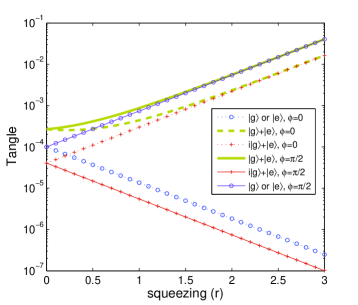
Figure 1: The tangle, Eq. (17), calculated for the atom and the squeezed light pulse mode bipartite system vs the squeezing strength. The pulse duration is $\tau=0.1\Gamma^{-1}$ and the coupling to the rest of the EM modes is neglected. The decay rate into paraxial modes is taken to be $\kappa=\Gamma/1000$. Results are shown for four atomic initial states and for the squeezing phases $\phi=0,\pi/2$, corresponding to amplitude and phase squeezing respectively. Compared with the coherent light case $(r=0)$, one obtains a squeezing-phase-dependent suppression and enhancement of the entanglement as squeezing gets larger.

III.2.3 Error probability calculation

The error probability of a quantum operation is just one minus the probability of the atomic qubit to be in the target state $|\eta\rangle$ of the operation after the operation is performed. A classical light pulse can be chosen to transform an atom from the initial to a prescribed final state $|\eta\rangle$. When operating with the quantized pulse, the operation is subject to quantum fluctuations. The fidelity $F$ is the probability of the atom to be in $|\eta\rangle$ after the quantized field has operated on it, $F=\langle\eta|\hat{\rho}_{A}|\eta\rangle$, where $\hat{\rho}_{A}$ is the density matrix that describes the, generally mixed, final state of the two-level atomic system. The error probability is then,

$$P_{error}=1-F=1-\langle\eta|\hat{\rho}_{A}|\eta\rangle.$$ (21)

Since in the absence of the reservoir the sole error is that due to atom-pulse entanglement, we were able to find a simple analytic relation between the tangle and the error probability calculated up to $O(\lambda^{2})$, $T\approx 4P_{error}$. This linear relation implies that the results for $P_{error}$ follow similar trends to those for the tangle and are squeezing phase and initial atomic state dependent (Fig. 2). For quantum information processing purposes the relevant error is that averaged over all possible atomic initial states, $<P_{error}>$. The averaged error is calculated analytically using the fidelity of 6 different initial atomic states avF

$$<P_{error}>\approx\left(0.0675e^{\pm 2r}+0.1665e^{\mp 2r}\right)\kappa\tau,$$ (22)

where as before the upper (lower) sign is for $\phi=0$ ($\phi=\pi/2$). This result is plotted as a function of squeezing in Fig. 3. As can be seen the averaged error, $<P_{error}>$, depends on the squeezing phase $\phi$. For most values of the squeezing parameter $r$ the average error is larger than in the CL case ($r=0$). This implies that on average, more entanglement is generated between the atom and the pulse in SL than in CL case. Still one observes that for the region $0<r<0.45$, and $\phi=0$ (amplitude squeezing), the average error drops relative to the error in the CL case. Though practically small, in this range of the squeezing parameter the SL operation has lower quantum limit to the operation error than with the CL pulse due to reduced intensity noise.

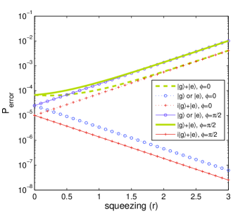
Figure 2: The error probability of an operation with a squeezed light $\pi$ pulse on an atom vs squeezing strength. The pulse duration is $\tau=0.1\Gamma^{-1}$ and the rest of the EM modes are disregarded. As in Fig. 1, $\kappa=\Gamma/1000$ is taken. The inset shows the atomic initial states and the squeezing phase. Here $\phi=0$ ($\pi/2$) corresponds to reduced amplitude (phase) fluctuations. The dependence on the squeezing phase follows the results for the entanglement. Lower errors than for the coherent light operation ($r=0$) can be achieved.

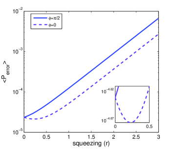
Figure 3: Same as Fig. 2, but for the average error probability. The average is over all possible atomic initial states. For most cases, the average error with squeezed light increases relative to coherent light ($r=0$). For the squeezing phase $\phi=0$ (amplitude squeezing) and squeezing strength $0<r<0.45$ a very small decrease in the average error is observed, as shown in the figure inset.

III.2.4 Discussion of the results

4a. Quantum interference
Consider the interaction $\hat{W}$ between the atom and the fluctuating part of the light pulse shown in Eq. (12). In addition to the Jaynes-Cummings like atom-photon interaction term $\hat{W}_{1}\equiv i(\hat{a}\hat{\sigma}_{+}-h.c.)$, present also in the CL case, it contains a squeezing-dependent term $\hat{W}_{2}\equiv i\left[(s/c)e^{-2\varphi}\hat{\sigma}_{+}\hat{a}^{{\dagger}}-h.c.\right]$. Atomic and light mode excitations can be generated via both $\hat{W}_{1}$ and $\hat{W}_{2}$. These two paths interfere quantum mechanically resulting a dependence of atom-light entanglement and error probability on both squeezing and atomic phases.

Starting from $|g,0\rangle$ we examine the bipartite state evolution under the first two operators in Eq. (16). The classical field term, $\hat{U}^{(0)}$, is evolving the state to $|e,0\rangle$ via superpositions of $|g,0\rangle$ and $|e,0\rangle$. Simultaneously the state evolves under the term $\hat{W}$ in $\hat{U}^{(1)}$. The $\hat{W}_{1}$ part of it couples only to $|e,0\rangle$ evolving it to $|g,1\rangle$. The $\hat{W}_{2}$ part on the other hand couples only to $|g,0\rangle$ and transform it to $|e,1\rangle$. Subsequent evolution under $\hat{U}_{0}$ forms superpositions of $|e,1\rangle$ and $|g,1\rangle$, the amplitudes of which are coherent sums (and therefore show interference) of evolution amplitudes under both $\hat{W_{1}}$ and $\hat{W_{2}}$. Quantitatively,

$$|\psi(\tau)\rangle\approx\left[\hat{U}^{(0)}+\lambda\hat{U}^{(1)}\right]|g,0\rangle=$$

$$|e,0\rangle+\lambda\int_{0}^{1}d\xi\hat{U}_{0}(1-\xi)(\hat{W}_{1}+\hat{W}_{2})\hat{U}_{0}(\xi)|g,0\rangle=$$

$$|e,0\rangle-\lambda\int_{0}^{1}d\xi\hat{U}_{0}(1-\xi)\sin\left(\frac{\pi}{2}\xi\right)|g,1\rangle-$$

$$\lambda\int_{0}^{1}d\xi\hat{U}_{0}(1-\xi)e^{-i2\phi}\frac{s}{c}\cos\left(\frac{\pi}{2}\xi\right)|e,1\rangle=$$

$$|e,0\rangle-\lambda\frac{1}{\pi}\left(e^{-i2\phi}\frac{s}{c}+1\right)|e,1\rangle+\lambda\frac{1}{2}\left(e^{-i2\phi}\frac{s}{c}-1\right)|g,1\rangle,$$

(23)

where $\hat{U}_{0}(\xi)|g/e,0\rangle=\cos\left(\frac{\pi}{2}\xi\right)|g/e,0\rangle\pm\sin\left(\frac{\pi}{2}\xi\right)|e/g,0\rangle$.
The interference between evolution under $\hat{W}_{1}$ and $\hat{W}_{2}$ is clearly seen in the amplitudes of $|e,1\rangle$ and $|g,1\rangle$. For large squeezing, i.e. $s\cong c$, and $\phi=0$, we get $|e\rangle\otimes\left(|0\rangle-\frac{2}{\pi}\lambda|1\rangle\right)$ which contains no entanglement. For $\phi=\pi/2$ we get $|e,0\rangle+\lambda|g,1\rangle$ which is entangled with entanglement strength on the order of the interaction strength $\lambda$. This result is similar to that obtained for the tangle in III B2. For other atomic initial states similar calculations up to second order in $\lambda$ were performed leading to the results shown in III B2 and III B3.

4b. Optical Bloch equation (OBE) with a noisy field
An intuitive understanding of the error results from Sec. III B can be obtained from the Bloch sphere picture. To this end we derive the OBE for a one mode SL field, starting from the Hamiltonian (8), $\hat{H}=i\hbar g\left[(\hat{a}+\alpha)\hat{\sigma}_{+}-(\hat{a}^{{\dagger}}+\alpha^{\ast})\hat{\sigma}_{-}\right]$. As usual for SL, we define the quadrature operators $\hat{X}_{1,2}=\hat{\delta X}_{1,2}+x_{1,2}$ with

$$\hat{a} \equiv \frac{1}{2}\left(\hat{\delta X}_{1}+i\hat{\delta X}_{2}\right)$$

$$\alpha \equiv \frac{1}{2}\left(x_{1}+ix_{2}\right).$$ (24)

Here $\hat{\delta X}_{1,2}$ are hermitian operators with zero average and $x_{1,2}$ are real numbers representing the averages of the quadratures. We then define the vectors

$$\vec{x} \equiv \left(x_{2},x_{1},0\right)$$

$$\hat{\vec{\delta X}} \equiv \left(\hat{\delta X}_{2},\hat{\delta X}_{1},0\right),$$ (25)

so that the Hamiltonian (8) becomes

$$\hat{H}=-\hbar\frac{g}{2}\left(\vec{x}+\hat{\vec{\delta X}}\right)\cdot\hat{\vec{\sigma}},$$ (26)

with $\hat{\vec{\sigma}}=(\hat{\sigma}_{x},\hat{\sigma}_{y},\hat{\sigma}_{z})$. The resulting Heisenberg equation for $\hat{\vec{\sigma}}(t)$ is

$$\frac{d\hat{\vec{\sigma}}}{dt}=-\frac{g}{2}\vec{x}\times\hat{\vec{\sigma}}-\frac{g}{2}\hat{\vec{\delta X}}\times\hat{\vec{\sigma}},$$ (27)

with all the operators written in the Heisenberg picture. Rescaling the time to $\bar{t}=t/\tau$ Eq. (27) becomes

$$\frac{d\hat{\vec{\sigma}}}{d\bar{t}}=-\vec{\Omega}\times\hat{\vec{\sigma}}-\frac{1}{2}\zeta\hat{\vec{\delta X}}\times\hat{\vec{\sigma}},$$ (28)

where $\vec{\Omega}=(g\tau\vec{x}/2)$ is the dimensionless Rabi vector and $\zeta=g\tau$. Recall that for a $\pi$ pulse $|\alpha|=(\pi/2g\tau)$ and therefore $|\vec{\Omega}|=O(1)$. Our calculation also assumes $\lambda=\cosh(r)\zeta\ll 1$, i.e. even for matrix elements of $\hat{\vec{\delta X}}$ which are of order $\cosh(r)$, $\zeta\hat{\vec{\delta X}}$ is still very small. We can then expand the operators $\hat{\vec{\sigma}}(\bar{t})=\hat{\vec{\sigma}}_{0}(\bar{t})+\zeta\hat{\vec{\sigma}}_{1}(\bar{t})+...$ and $\hat{\vec{\delta X}}(\bar{t})=\hat{\vec{\delta X}}_{0}(\bar{t})+\zeta\hat{\vec{\delta X}}_{1}(\bar{t})+...$, to obtain to first order in $\zeta$,

$$\frac{d\hat{\vec{\sigma}}}{d\bar{t}}\approx-\vec{\Omega}\times\hat{\vec{\sigma}}-\frac{1}{2}\zeta\hat{\vec{\delta X}}_{0}\times\hat{\vec{\sigma}}_{0}.$$ (29)

The last term includes the cross product of the Heisenberg picture operators in the absence of atom-field interaction, so that $\hat{\vec{\sigma}}_{0}(\bar{t})$ is simply the solution of the OBE with the classical field $\vec{\Omega}$ and describes evolution in the atomic part of the Hilbert space, and $\hat{\vec{\delta X}}_{0}=\hat{\vec{\delta X}}(\bar{t}=0)$ is in the photonic part of the Hilbert space.

The average over atomic degree of freedom can be defined on any operator $\hat{O}$ to be $\langle\hat{O}\rangle_{A}\equiv\mathrm{tr_{A}}[\hat{\rho_{A}}\hat{O}]$, where $A$ denotes the atom system and $\hat{\rho_{A}}$ is the reduced atomic density operator. Averaging equation (29) this way we get an OBE with a noisy field,

$$\frac{d\langle\hat{\vec{\sigma}}\rangle_{A}}{d\bar{t}}\approx-\vec{\Omega}\times\langle\hat{\vec{\sigma}}\rangle_{A}-\frac{1}{2}\zeta\hat{\vec{\delta X}}_{0}\times\langle\hat{\vec{\sigma}}_{0}\rangle_{A}.$$ (30)

Note that $\langle\hat{\vec{\sigma}}\rangle_{A}(\bar{t})$ and $\hat{\vec{\delta X}}_{0}$ are operators in the photonic space and are therefore fluctuating, whereas $\langle\hat{\vec{\sigma}}_{0}\rangle_{A}(\bar{t})$ is just the c-number Bloch vector solution of an OBE driven by the average field $\vec{\Omega}$ and it in fact equals to the average of $\hat{\vec{\sigma}}(\bar{t})$ over both atomic and photonic degrees of freedom. The term with $\hat{\vec{\delta X}}_{0}$ is the one driven by the fluctuations of the field, which in our case are quadrature dependent SL fluctuations. For $\phi=0$, the uncertainties of the quadratures are $\Delta\hat{\delta X}_{1}=e^{-r}\leq 1$ and $\Delta\hat{\delta X}_{2}=e^{r}\geq 1$, i.e. $\hat{\delta X}_{1}$ has reduced fluctuations and $\hat{\delta X}_{2}$ has increased fluctuations relative to CL. For $\phi=\pi/2$ we get the opposite.

We can now present the field in the Bloch sphere as seen in Fig. 4. Taking real $\alpha$ $(\theta=0)$ and squeezing phase $\phi=0$, the Rabi vector is pointing to the $y$ direction $(x_{2}=0)$ and is amplitude squeezed ($\Delta\hat{\delta X}_{1}<1$). Now consider an initial ground state, i.e. $\langle\hat{\vec{\sigma}}\rangle_{A}$ is pointing to the $-z$ direction. For a $\pi$ pulse operation, the $xy$ phase of the field is not relevant, and therefore phase noise of the field doesn’t affect the operation. The only relevant noise is the amplitude noise which for $\phi=0$ is reduced relative to CL case. We thus expect to get a lower error in this operation as compared with the CL operation. For $\phi=\pi/2$, the field has an increased amplitude noise ($\Delta\hat{\delta X}_{1}>1$), which results an increased error compared to the CL case. Now consider the $y$ axis pointing initial state again for $\theta=0$. Since the Rabi vector is also pointing to the $y$ direction the average ”moment” obtained from the cross product is zero. Here only the $\hat{\delta X}_{2}$ ”phase” noise, in the $x$ direction, affects the qubit state. When this noise is increased ($\phi=0$) the error is larger than in the CL case, and when it is reduced ($\phi=\pi/2$) the error gets lower. For an initial state pointing to the $x$ direction, one can see that in general, both $\hat{\delta X}_{2}$ and $\hat{\delta X}_{1}$ affect the operation, and therefore squeezing in any quadrature typically increases the operation error.

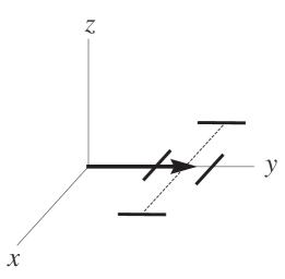
Figure 4: The driving field in the optical Bloch equation representation. The solid arrow is the Rabi vector $\vec{\Omega}$ proportional to $\vec{x}$ from Eq. (25) for $x_{2}$=0 ($\theta=0$). The error bars are the variances of the field fluctuations $\Delta\hat{\delta X}_{2}$ and $\Delta\hat{\delta X}_{1}$ in the $x$ and $y$ directions respectively. Here $\phi=0$ is taken, i.e. $\Delta\hat{\delta X}_{1}<\Delta\hat{\delta X}_{2}.$

III.3 Entanglement and error probability calculations in the presence of the reservoir

We now wish to examine how accounting for the spontaneous emission into the reservoir of empty modes will modify the above results. To this end the full master equation, Eq. (13), has to be solved. We again assume $\lambda\ll 1$ and work in the truncated basis $\left\{|g,0\rangle,|g,1\rangle,|e,0\rangle,|e,1\rangle\right\}$. We solve Eq. (13) numerically in this basis using $\kappa=\Gamma/1000$ and calculate the density matrix $\hat{\rho}(\tau)$ of the bipartite final state. We then use $\hat{\rho}(\tau)$ to evaluate the tangle and the error probability.

III.3.1 Tangle calculation

Within the truncated basis, the pulse mode is also a two-level system. We follow osborne ; wooters where a procedure for the tangle calculation of a two-qubit mixed state is given. Figure 5 presents the tangle as a function of the pulse duration $\tau$. We assume squeezing of $r=1.16$, which corresponds to $10\log_{10}(e^{2r})=10\mathrm{dB}$ pulse mode quadrature noise reduction. The interaction with the reservoir changes atom-pulse entanglement when $\Gamma\tau\gtrsim 1$ and should generally decrease it for $\Gamma\tau\gg 1$. Whenever the tangle is not suppressed by the SL operation, pulses shorter than $0.1\Gamma^{-1}$ are well accounted by neglecting the reservoir, i.e. extending the initial linear part of the plots. When SL operation suppresses the entanglement, the interaction with the reservoir becomes more dominant, and the effect of the reservoir can only be neglected for pulses shorter than $0.01\Gamma^{-1}$.

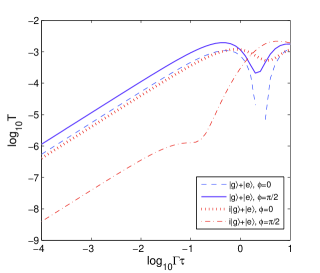
Figure 5: The tangle generated between the atom and the squeezed light pulse mode as a function of the pulse duration scaled to atom free space decay time $\Gamma^{-1}$. The squeezing of the pulse mode is taken to be $r=1.16$, which corresponds to $10\log_{10}(e^{2r})=10\mathrm{dB}$ quadrature noise reduction. As in Fig. 1, $\kappa=\Gamma/1000$ is taken. The reservoir of the free space EM modes is included. Results for two atomic initial states are plotted. The effect of the reservoir is seen in the deviation from the initial linear part of the plots. This deviation begins as expected at times slightly shorter than $\tau\sim\Gamma^{-1}$, when entanglement is enhanced by SL (all cases here, apart from $i|g\rangle+|e\rangle$, $\phi=\pi/2$). When entanglement is suppressed by SL, the effect of the reservoir is seen already at much smaller $\tau$.

III.3.2 Error probability calculation

The error probability is calculated using Eq. (21). Figure 6 shows the results for $\tau=0.1\Gamma^{-1}$ pulse duration. Let us now compare between Fig. 6 and Fig. 2, where the reservoir has been neglected. We focus on the case of the initial state $\frac{1}{\sqrt{2}}\left(i|g\rangle+|e\rangle\right)$. For $r=0$, i.e. a CL pulse, the error of about $0.0244$ seen in the left hand part of Fig. 6 is actually due to spontaneous emission to all the EM modes, as can be understood from the Mollow picture (see Ref. itano ). The corresponding error in Fig. 2 is only $10^{-5}$. This suggests that owing to its small solid angle ($\kappa=\Gamma/1000$), the error due to coupling to the laser mode is overwhelmed by that due to coupling to the reservoir modes. When squeezing is introduced ($r>0$), for $\phi=\pi/2$, the atom-pulse entanglement is suppressed as seen in Fig. 2. This suppression is hardly noticeable when the reservoir modes are included as one can see from Fig. 6. Numerically, for $r=3$, we find that the error decrease is $0.95\times 10^{-5}$. This matches what could be expected from Fig. 2 and demonstrates that the reservoir is the major cause of error in this case. On the other hand, for $\phi=0$, an increase of the error seen in Fig. 2 persists also in the presence of the reservoir, as can be seen in Fig. 6. For very large squeezing this increase may become of the same order of magnitude as the error due to the spontaneous emission to all the EM modes. E.g. for $r=3$ the increase seen in both Figs. 2 and 6 is $\sim 4\times 10^{-3}$, about $16.3\%$ of the $0.0244$ error induced by spontaneous emission.

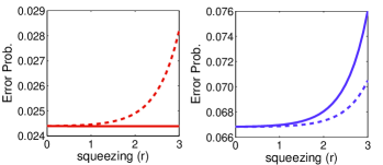
Figure 6: The error probability of an operation with a squeezed light $\pi$ pulse on an atom vs squeezing strength. The pulse duration is $\tau=0.1\Gamma^{-1}$ and atomic decay into all the reservoir modes is considered. As in Fig. 1, $\kappa=\Gamma/1000$ is taken. The left plot is the calculation for $i|g\rangle+|e\rangle$ atom initial state and the right one is for $|g\rangle+|e\rangle$. The dashed lines are for $\phi=0$ and the solid lines for $\phi=\pi/2$.

IV Discussion

The results of Sec. III show that the entanglement between the pulse mode and the atom is indeed modified in a squeezing-phase-dependent way. However, the use of squeezed light would not reduce the average error compared with the CL case by a practicably useful amount. Despite its inapplicability for Quantum computing, the entanglement between SL and a single atom is of scientific interest, and would be interesting if observed experimentally.

Contrary to CL, where atom-light entanglement is probably too small to be detected, SL with a large squeezing parameter $r$ and a right choice of phases, will eventually enhance SL-atom entanglement to experimentally detectable values. A direct measurement of entanglement would be through complete state tomography of the combined SL-atom state. The tangle would then be calculated from the reconstructed density matrix. The requirements for this experiment would be a squeezed light source with a sufficiently large squeezing parameter squeezing-bandwidth , atomic state detection and photodetectors with sufficient efficiency. Alternatively, ignoring the light mode, the error in the final atomic state can be measured for various parameters, such as different squeezing phases, thus relaxing the need for an efficient photodetector.

Examples for squeezed light sources include four wave mixing in a nonlinear medium, optical parametric amplifiers, second harmonic generation and amplitude squeezed light from diode lasers among others Bachor . All these sources can be pulsed, e.g. via electro-optic modulators. The initial light state we assumed for the control field was a single-mode squeezed state. Parametric down conversion (PDC) of short pulses could be considered as one example of a realization for such a light source. In boyd ; wasilewski the multimode pulsed SL produced by PDC is analyzed and described by a discrete set of squeezed modes. In fact, for some conditions of phase matching and pump pulse duration, only one of the modes of the discrete set is squeezed, resulting in a pulse in a single-mode squeezed state.

Even the most advanced single-mode squeezed light sources to-date cannot reach quadrature noise suppression greater than $10$dB ($r=1.16$) Bachor . This means that the maximal error increase and tangle expected and therefore the minimal required detection error, will be of the order of a few $10^{-4}$ (see Fig. 1 and 2). Current state-of-the-art atomic state detection has an error which is of similar magnitude Langer ; Oxford . However the efficiency of even the most advanced photodetectors is far from satisfying such low error rates. It therefore seems that a direct tangle measurement is currently unfeasible, however, an indirect indication for entanglement, detected through gate error enhancement, is within experimental reach.

One important limitation for observing the error modification effects in free space is the spacial overlap between the atom and the paraxial pulse mode. Similar limitations make up a major difficulty in observing the effect of the inhibition of the atom coherences decay in a squeezed vacuum reservoir, found by Gardiner gar86 . In this context, other schemes, involving atom-squeezed vacuum interaction in a cavity, were considered ParZollerCar . Recent theoretical analysis and experiment however have shown a possibility of strong coupling of a laser mode to a single atom in free space vanEnkKimble2000 ; Kurtsiefer ; Agio . The use of such beams, where the overlap between the incoming beam and the atomic dipole radiation pattern is large ($\kappa\sim\Gamma$), may greatly enhance the effects discussed above.

In many experiments, a pair of ground, e.g. hyperfine, states of an atomic system is used as a qubit. Although the energy separation between ground states is typically in the radio-frequency range, quantum gates are often driven with a laser beam pair, off-resonance with a third optically excited level, in a Raman configuration. The limitations to hyperfine qubit coherence and gate fidelity due to the quantum nature of the Raman laser fields was investigated both experimentally and theoretically Ozeri 2005 ; Ozeri 2007 . In this case too, it is interesting to ask whether the use of, either independently or relatively, squeezed light fields would influence the gate error. An experiment, similar to that described above, but with a ground state qubit could benefit from the ground state qubit intrinsic longevity. In fact, a gate averaged error of few $10^{-3}$, dominated by laser classical noise and photon scattering, was recently measured on a single trapped-ion hyperfine qubit and a Raman laser gate Knill 2008 .

To conclude, we have calculated the entanglement between a short pulse of resonant squeezed light and a two-level atom in free space during a qubit $i\hat{\sigma}_{y}$ gate (a $\pi$ pulse) and the resulting gate error. Several differences arise when comparing to coherent control with CL. As could be expected for squeezed light, three phases determine the error magnitude - the squeezing phase, the light phase and the phase of the initial qubit superposition. In comparison with the coherent light case, the error and the entanglement can be either enhanced or suppressed depending on the above phase relations. These entanglement enhancement and suppression effects naturally become stronger with squeezing and can get to a few orders of magnitude. For quantum information processing purposes the relevant error is that averaged over all possible initial states. We have shown that although in principal the average error can be reduced by using SL within a specific range of parameters, the resulting minimum error however would be of the same order of magnitude as that with CL. In fact, even when not averaged, but when taking into account the free space environment, the error is still mostly dominated by the atomic decay to the EM reservoir owing to a very small atom-pulse spacial overlap, so that any reduction is not likely do be detected experimentally. On the other hand, the effect of enhanced atom-pulse entanglement is of scientific interest and might even prove useful as a resource in some quantum communication schemes. A measurement of the increased error would be an indirect indication for the enhancement of entanglement by squeezing.

Appendix A Quantized Paraxial Approximation

Here we would like to derive the model Hamiltonian of the atom-pulse mode interaction in free space seen in Eq. (2). We start from the usual atom-field Hamiltonian in the dipole approximation

$$\hat{H} = \hat{H}_{F}+\hat{H}_{A}+\hat{H}_{AF}$$

$$\hat{H}_{F} = \sum_{\vec{k}\mu}\hbar\omega_{k}\hat{a}^{\dagger}_{\vec{k}\mu}\hat{a}_{\vec{k}\mu}$$

$$\hat{H}_{A} = \frac{1}{2}\ \hbar\omega_{a}\hat{\sigma}_{z}$$

$$\hat{H}_{AF} = \sum_{\vec{k}\mu}i\sqrt{\frac{\hbar\omega_{k}}{2\epsilon_{0}}}d_{\hat{k}\mu}\left(\hat{a}_{\vec{k}\mu}\frac{e^{i\vec{k}\cdot\vec{r}_{a}}}{\sqrt{V}}-h.c.\right)\left(\hat{\sigma}_{+}+\hat{\sigma}_{-}\right),$$

where $\vec{k}\mu$ are the indices of a Fourier mode and its polarization respectively, and $\vec{r}_{a}$ is the position of the atom. The dipole matrix element $\vec{d}$ is assumed to be real and $d_{\hat{k}\mu}=\vec{\varepsilon}_{\hat{k}\mu}\cdot\vec{d}$, where $\vec{\varepsilon}_{\hat{k}\mu}$ is the polarization vector with polarization $\mu$ and is perpendicular to the propagation direction $\vec{k}$. We first divide the sums on Fourier modes into the paraxial subspace modes, $\Lambda_{p}$, and the nonparaxial subspace modes. The paraxial subspace modes include the modes centered around some carrier wave vector in the $z$ direction $\vec{k}_{0}=k_{0}\vec{z}$:

$$\Lambda_{p} = \{\Lambda_{p}^{x},\Lambda_{p}^{y},\Lambda_{p}^{z}\}$$

$$\Lambda_{p}^{x} = (-k_{x}^{co},k_{x}^{co})$$

$$\Lambda_{p}^{y} = (-k_{y}^{co},k_{y}^{co})$$

$$\Lambda_{p}^{z} = (k_{0}-k_{z}^{co},k_{0}+k_{z}^{co}),$$ (32)

where the bandwidths for (x,y,z) directions are narrow, i.e.

$$k_{i}^{co}\ll k_{o}$$

$$i=x,y,z.$$ (33)

The nonparaxial modes are simply the rest of the modes $\vec{k}\mu$ not included in $\Lambda_{p}$ and we denote them with indices $\{q\}$. The paraxial subspace $\Lambda_{p}$ can be approximately spanned by the modes which are the solutions of the paraxial wave equations in free space with carrier frequencies $\omega_{k}=(k_{0}+k)c$, $TEM_{nm}^{k_{0}+k}$. These modes are denoted by the functions $U_{nmk}(\vec{r})=u_{nmk}(\vec{r})e^{i(k_{0}+k)z}$. Their Fourier coefficients are $U_{nmk}(\vec{k})$ so that their mode operators are

$$\hat{a}_{nmk,\mu}=\sum_{\vec{k}\in\Lambda_{p}}U_{nmk}^{\ast}(\vec{k})\hat{a}_{\vec{k}\mu}\Rightarrow\hat{a}_{\vec{k}\mu}=\sum_{nmk}U_{nmk}(\vec{k})\hat{a}_{nmk,\mu}.$$ (34)

Note that the Fourier modes here, $\hat{a}_{\vec{k}\mu}$, are only those included in the paraxial subspace. Using (34) it is easy to show within the paraxial approximation that

$$\sum_{\vec{k}\mu}\sqrt{\omega_{k}}d_{\hat{k}\mu}\hat{a}_{\vec{k}\mu}\frac{e^{i\vec{k}\cdot\vec{r_{a}}}}{\sqrt{V}}\approx\sqrt{\omega_{0}}\sum_{nmk,\mu}d_{\mu}\hat{a}_{nmk,\mu}U_{nmk}(\vec{r}_{a}),$$ (35)

where $\omega_{0}=k_{0}c$. We denote all the $\{nm\neq 00,k,\mu\}$ and $\{nm=00,k,\mu=2\}$ modes by $\{i\}$, where $\{\mu\}=\{1,2\}$ are the two polarizations. The rest of the modes ,$\{nm=00,k,\mu=1\}$, have Gaussian transverse profile and are denoted $\{k\}$. We thus get

$$\hat{H}_{AF} = i\hbar\sum_{q}\left(g_{q}\hat{a}_{q}-g_{q}^{\ast}\hat{a}_{q}^{\dagger}\right)\left(\hat{\sigma}_{+}+\hat{\sigma}_{-}\right)+$$

$$i\hbar\sum_{i}\left(g_{i}\hat{a}_{i}-g_{i}^{\ast}\hat{a}_{i}^{\dagger}\right)\left(\hat{\sigma}_{+}+\hat{\sigma}_{-}\right)+$$

$$i\hbar\sum_{k}\left(\sqrt{\frac{\omega_{0}}{2\epsilon_{0}\hbar}}dU_{00k}(\vec{r_{a}})\hat{a}_{k}-h.c\right)\left(\hat{\sigma}_{+}+\hat{\sigma}_{-}\right),$$

where $d=d_{\mu=1}$ and $g_{i}$, $g_{q}$ are the atom-mode dipole couplings for the modes $\{i,q\}$. The dipole couplings for the $\{k\}$ modes are seen explicitly in (LABEL:H_tot_gk),

$$g_{k}=\sqrt{\frac{\omega_{0}}{2\epsilon_{0}\hbar}}dU_{00k}(\vec{r}_{a})=\sqrt{\frac{\omega_{0}}{2\epsilon_{0}\hbar}}du_{00k}(\vec{r}_{a})e^{i(k_{0}+k)z_{a}}.$$ (37)

We note that $u_{00k}(\vec{r}_{a})$ is just the overlap of the $k$ mode with the atom. This overlap includes some normalization of a quantization length in the beam direction, $L$, which should eventually be taken to be infinity, and which is multiplied by some effective area of the mode, $A$, evaluated at the atom’s position, i.e. $u_{00k}(\vec{r_{a}})=1/\sqrt{AL}$. Considering the narrow band of $k$ values around $k_{0}$, $A$ is approximately independent of $k$. The couplings $g_{k}$ are then written

$$g_{k}=d\sqrt{\frac{\omega_{0}}{2\epsilon_{0}\hbar A}}\frac{1}{\sqrt{L}}e^{i(k_{0}+k)z_{a}}.$$ (38)

As for $\hat{H}_{F}$, since all the modes discussed here, $\{q,i,k\}$, are eigenmodes of free space in the paraxial approximation, they have well-defined single-particle energies $\hbar\omega_{q}$, $\hbar\omega_{i}$ and $\hbar\omega_{k}$ respectively. The total Hamiltonian from Eq. (LABEL:H_tot_k) thus becomes

$$\hat{H} = \hat{H}_{F}+\hat{H}_{A}+\hat{H}_{AF}$$

$$\hat{H}_{F} = \sum_{q}\hbar\omega_{q}\hat{a}^{\dagger}_{q}\hat{a}_{q}+\sum_{i}\hbar\omega_{i}\hat{a}^{\dagger}_{i}\hat{a}_{i}+\sum_{k}\hbar\omega_{k}\hat{a}^{\dagger}_{k}\hat{a}_{k}$$

$$\hat{H}_{A} = \frac{1}{2}\ \hbar\omega_{a}\hat{\sigma}_{z}$$

$$\hat{H}_{AF} = i\hbar\sum_{j=\{q,i,k\}}\left(g_{j}\hat{a}_{j}-g_{j}^{\ast}\hat{a}_{j}^{\dagger}\right)\left(\hat{\sigma}_{+}+\hat{\sigma}_{-}\right).$$ (39)

We would now like to describe a pulse mode with a Gaussian transverse profile composed of Gaussian beams of different frequencies around the carrier frequency $\omega_{0}$. The pulse mode is then spanned by the $\{k\}$ modes. We can choose a new orthonormal basis $\{f\}$ which spans the same subspace as that of the $\{k\}$ basis and that includes a pulse mode $f_{0}$ as one of its members. Both $\{k\}$ and $\{f\}$ modes share a similar Gaussian $xy$ profile, we therefore focus only on their $z$ dependence. We write the relation between the $k$ and $f$ mode functions as

$$\Phi_{f}(z)=e^{ik_{0}z}\varphi_{f}(z)=e^{ik_{0}z}\sum_{k}\varphi_{f}(k)\frac{e^{ikz}}{\sqrt{L}},$$ (40)

where $e^{i(k_{0}+k)z}/\sqrt{L}$ is a $k$ mode while $\Phi_{f}(z)$ is an $f$ mode. An $f$ mode is thus defined by its envelope $\varphi_{f}(z)$. In a similar way, the transformation for the field operators is

$$\hat{a}_{k}=\sum_{f}\varphi_{f}(k)\hat{a}_{f}.$$ (41)

The pulse mode is then characterized by the operator $\hat{a}_{f_{0}}$, whereas the Hilbert space of the two-level atom is spanned by the Pauli spin matrices. The atom and the pulse mode make for the relevant bipartite system. The rest of the EM modes, $\hat{a}_{f\neq f_{0}}$, $\hat{a}_{i}$ and $\hat{a}_{q}$, interact with the bipartite system via the atom and make up a reservoir.

We now focus on the part of the Hamiltonian that includes only the atom and the Gaussian paraxial modes $\{k\}$, and their interaction

$$\hat{H}^{p} = \sum_{k}\hbar\omega_{k}\hat{a}^{\dagger}_{k}\hat{a}_{k}+\frac{1}{2}\hbar\omega_{a}\hat{\sigma}_{z}+$$ (42)

$$i\hbar\sum_{k}\left(g_{k}\hat{a}_{k}-h.c.\right)\left(\hat{\sigma}_{+}+\hat{\sigma}_{-}\right).$$

Moving to the interaction picture in the rotating wave approximation, assuming no detuning ($\omega_{a}=\omega_{0}$) and using equations (38, 40, 41), we get

$$\hat{H}_{I}^{p}=i\hbar\sum_{f}\left[\ g_{f}(t)\hat{a}_{f}\hat{\sigma}_{+}-h.c.\right],$$ (43)

with

$$g_{f}(t)=d\sqrt{\frac{\omega_{0}}{2\epsilon_{0}\hbar A}}e^{ik_{0}z_{a}}\varphi_{f}(z_{a}-ct).$$ (44)

The system Hamiltonian of the relevant bipartite system comprised of the atom and the pulse mode is then

$$\ \hat{H}_{S}\equiv\hat{H}_{I}^{f_{0}+atom}=i\hbar g_{f_{0}}(t)\left[\ \hat{a}_{f_{0}}\hat{\sigma}_{+}-h.c.\right],$$ (45)

where we take the envelope of the pulse, $\varphi_{f_{0}}(z)$, to be real and set $z_{a}=0$. Denoting all the rest the EM modes apart from $f_{0}$ with indices $\{r\}$ we get the total Hamiltonian in the interaction picture in Eq. (2).

References

- (1) E. Knill, Nature 434, 39 (2005).
- (2) S. J. van Enk and H. J. Kimble, Quantum Inf. Comput. 2, 1 (2002).
- (3) J. Gea-Banacloche, Phys. Rev. A, 65, 022308 (2002).
- (4) A. Silberfarb and I. H. Deutsch, Phys. Rev. A, 68, 013817 (2003).
- (5) W. M. Itano, Phys. Rev. A, 68, 046301 (2003).
- (6) A. Silberfarb and I. H. Deutsch, Phys. Rev. A, 69, 042308 (2004).
- (7) H. Nha and H. J. Carmichael , Phys. Rev. A, 71, 013805 (2005).
- (8) C. M. Caves , Phys. Rev. D, 23, 1693 (1981).
- (9) P. Grangier, R. E. Slusher, B. Yurke and A. LaPorta , Phys. Rev. Lett., 59, 2153 (1987).
- (10) T. C. Ralph, Phys. Rev. A, 61, 010303(R) (1999)
- (11) M. Hillery, Phys. Rev. A, 61, 022309 (2000)
- (12) D. Gottesman and J. Preskill, Phys. Rev. A, 63, 022309 (2001).
- (13) B. J. Dalton, Z. Ficek and S. Swain, J. Mod. Opt. 46, 379 (1999).
- (14) B. J. Dalton and Z. Ficek (Eds.), Quantum Squeezing (Springer-Verlag, Berlin Heidelberg, 2004).
- (15) C. W. Gardiner, Phys. Rev. Lett. 56, 1917 (1986).
- (16) H. J. Charmichael, A. S. Lane and D. F. Walls, J. Mod. Opt. 34, 821 (1987).
- (17) A. S. Parkins and C. W. Gardiner, Phys. Rev. A 37, 3867 (1988).
- (18) G. J. Milburn, J. Mod. Opt. 31, 671 (1984).
- (19) A. Aiello and J. P. Woerdman, Phys. Rev. A 72, 060101(R) (2005).
- (20) I. H. Deutsch and J. C. Garrison, Phys. Rev. A 43, 2498 (1991).
- (21) B. R. Mollow, Phys. Rev. A 12, 1919 (1975).
- (22) C. Cohen-Tannoudji, J. Dupont-Roc and G. Grynberg, Atom-Photon Interactions (Wiley, New York, 1992), p. 597.
- (23) E. Shahmoon, M.Sc. thesis, Weizmann Institute of Science, 2008.
- (24) T. J. Osborne, e-print quant-ph/0203087
- (25) W. K. Wootters, Phys. Rev. Lett. 80, 2245 (1998).
- (26) P. Rungta, V. Bužek, Carlton M. Caves, M. Hillery and G. J. Milburn, Phys. Rev. A 64, 042315 (2001).
- (27) M. D. Bowdrey, D. K. L. Oi, A. J. Short, K. Banaszek and J. A. Jones, Phys. Lett. A 294, 258 (2002).
- (28) Noise reduction below the SQL was typpically demonstrated at noise frequencies of above a few MHz, whereas at low frequencies noise was dominated by classical laser noise. Here, for the average error to remain small, noise reduction is necessary at low frequencies as well.
- (29) Hans-A. Bachor and Timothy C. Ralph, A Guide to Experiments in Quantum Optics (WILEY-VCH, Weinheim, 2004).
- (30) R. S. Bennink and R. W. Boyd, Phys. Rev. A 66, 053815 (2002).
- (31) W. Wasilewski, A. I. Lvovsky, K. Banaszek and C. Radzewicz, Phys. Rev. A 73, 063819 (2006).
- (32) C. Langer, Ph.D. thesis, University of Colorado, 2006.
- (33) A. H. Myerson et al., Phys. Rev. Lett. 100, 200502 (2008).
- (34) A. S. Parkins, P. Zoller and H. J. Carmichael, Phys. Rev. A 48, 758 (1993).
- (35) S. J. van Enk and H. J. Kimble, Phys. Rev. A 61, 051802(R) (2000).
- (36) M. K. Tey, Z. Chen, S. A. Aljunid, B. Chng, F. Huber, G. Maslennikov and C. Kurtsiefer, Nature Phys., 2008.
- (37) G. Zumofen, N. M. Mojarad, V. Sandoghdar, and M. Agio, Phys. Rev. Lett. 101, 180404 (2008).
- (38) R. Ozeri et. al., Phys. Rev. Lett. 95, 030403 (2005).
- (39) R. Ozeri et. al., Phys. Rev. A 75, 042329 (2007).
- (40) E. Knill et. al., Phys. Rev. A 77, 012307 (2008).