The distribution of AGN in a large sample of galaxy clusters

Abstract

We present an analysis of the X-ray point source populations in 182 Chandra images of galaxy clusters at $z>0.1$ with exposure time $>$10 ksec, as well as 44 non-cluster fields. Analysis of the number and flux of these sources, using a detailed pipeline to predict the distribution of non-cluster sources in each field, reveals an excess of X-ray point sources associated with the galaxy clusters. A sample of 148 galaxy clusters at $0.1<z<0.9$, with no other nearby clusters, show an excess of 230 cluster sources in total, an average of $\sim$1.5 sources per cluster. The lack of optical data for these clusters limits the physical interpretation of this result, as we cannot calculate the fraction of cluster galaxies hosting X-ray sources. However, the fluxes of the excess sources indicate that over half of them are very likely to be AGN, and the radial distribution shows that they are quite evenly distributed over the central 1 Mpc of the cluster, with almost no sources found beyond this radius. We also use this pipeline to successfully reproduce the results of previous studies, particularly the higher density of sources in the central 0.5 Mpc of a few cluster fields, but show that these conclusions are not generally valid for this larger sample of clusters. We conclude that some of these differences may be due to the sample properties, such as the size and redshift of the clusters studied, or a lack of publications for cluster fields with no excess sources. This paper also presents the basic X-ray properties of the galaxy clusters, and in subsequent papers in this series the dependence of the AGN population on these cluster properties will be evaluated.

In addition the properties of over 9500 X-ray point sources in the fields of galaxy clusters are tabulated in a separate catalogue available online or at www.sc.eso.org/$\sim$rgilmour.

1 Introduction

Studies of AGN host galaxies are key to understanding the physical mechanisms which trigger AGN activity, and govern the fueling rate of the central black hole. An important part of these studies is the external environment of the galaxies, which has long been known to have a significant link with the galaxy properties (e.g Hubble & Humason 1931). Correlations such as the morphology–density (Dressler, 1980) and star-formation – density (e.g. Gómez et al. 2003) relations are evidence of the significant transformations that are associated with galaxy clusters. If AGN activity is influenced by, for example, galaxy mergers or gravitational disruption of the host galaxy, then the number of AGN would also differ between galaxy clusters and the field, and within the cluster itself.

The first evidence of a link between AGN activity and environment came in 1978, when Gisler (1978) found a lack of emission-line galaxies in galaxy clusters relative to the field, which was confirmed by Dressler, Thompson & Shectman (1984) . More recently, large optical surveys have been used to identify the properties of a significant number of host galaxies, and hence compare AGN activity in the same type of host galaxy but different environment. Miller et al. (2003) find that optical AGN activity is independent of environment, but Wake et al. (2004) show that the level of clustering depends on AGN luminosity. Kauffmann et al. (2003) find that AGN with strong [OIII] emission avoid areas of high galaxy density. Best (2004) investigate the radio properties of these AGN, and find that the fraction of galaxies with radio-loud AGN increases dramatically with local galaxy density, but that all of these AGN have low [OIII] emission and so may not be seen in optical surveys.

Arguably the least biased method of detecting AGN currently is to use X-ray images, which have the added advantage that the vast majority of point sources are AGN. Not long after optical surveys identified a lack of emission-line galaxies in clusters, X-ray surveys began to find a surprisingly high number of point sources in fields with galaxy clusters (Bechtold et al. 1983; Henry & Briel 1991; Lazzati et al. 1998). With the advent of the Chandra X-ray telescope, with sub-arcsecond point sources, such studies were repeated for other clusters, with a range of results. Significant overdensities of point sources have been found in a number of fields with galaxy clusters at moderate redshifts (Cappi et al. 2001, z=0.5; Martini et al. 2002, z=0.15; Molnar et al. 2002, z=0.32; Johnson et al. 2003, z=0.83; Martini et al. 2006, $0.05<z<0.31$; D’Elia et al. 2004, z=0.5) and groups (Jeltema et al. 2001, $0.2<z<0.6$), but Molnar et al. also found a z=0.5 cluster without a significant overdensity. More recently, studies of significant samples of galaxy clusters by Cappelluti et al. (2005) (10 clusters, $0.24<z<1.2$), Ruderman & Ebeling (2005) (51 clusters, $0.3<z<0.7$), and Branchesi et al. (2007) (18 clusters, $0.25<z<1.01$) have all found significant overdensities of point sources over the full sample, but not necessarily in all individual fields. However, the ChaMP project (Kim et al., 2004) find no difference in the number density of sources in fields with $z>0.3$ clusters compared to those without clusters.

The calculated number of AGN per cluster varies significantly in these samples, even taking into account the different depths of the observations and the statistical variance in the number of background sources in each image. This is to be expected as the number of AGN per cluster is, of course, related to the cluster properties, such as the number of possible AGN host galaxies. However, due to the lack of optical data it is hard to draw any conclusions from these samples as to how, if at all, the cluster environment affects the AGN population. Optical imaging and spectroscopy can identify the X-ray detected AGN in the cluster, rather than relying on statistical background subtraction, and also reveal the distribution and number of normal cluster galaxies. This would allow the calculation of the fraction of cluster galaxies which host AGN, as a function of cluster radius or cluster size for example, shedding light on the physical mechanisms affecting AGN. On the other hand obtaining optical data for a large sample of galaxy clusters is time consuming, and any strong trend should be visible in the distribution of X-ray point sources in a large sample of cluster fields. A rough estimate of the cluster galaxy population can also be made from the extended X-ray gas. An analysis based purely on X-ray data can therefore be very useful, but is clearly inferior to a full spectroscopic analysis of a large sample of clusters, with X-ray and optical data.

Such a study was started by Martini et al. (2002), using optical data to identify X-ray detected AGN in galaxy clusters. Martini, Mulchaey & Kelson (2007) have confirmed optically that the fraction of galaxies hosting X-ray detected AGN does differ significantly between the eight clusters in their sample, implying that the cluster properties affect the number of AGN. Their spectroscopic data confirms between 2 and 10 AGN per cluster, with a range in AGN fractions that cannot be explained by Poissonian variations. The mean fraction for the whole sample is 5 per cent of galaxies with $M_{R}<-20$ hosting AGN with $L_{X}>10^{41}$ erg sec^-1. The wide variation in the number or fraction of X-ray AGN is also found when other studies with spectroscopic data are compared. For example Finoguenov et al. (2004) find only one confirmed X-ray AGN, with luminosity $\sim 10^{41}$ erg sec^-1, in a 1.8 square degree survey of the centre of the Coma cluster (z=0.02), but Davis et al. (2003) find between 3 and 5 AGN in a cluster at z=0.08, giving a fraction of 4 per cent in agreement with the mean value of Martini et al.

Martini et al. also find tentative evidence that the clusters with higher AGN fraction have lower redshift, lower velocity dispersion, higher substructure and lower Butcher–Oemler (Butcher & Oemler, 1984) fraction, but due to the small size of the sample (8 clusters) it is not clear from this sample which, if any, of these factors is affecting the AGN activity. A higher AGN fraction at high redshift would be expected from the field evolution of AGN, but no strong evolution is found by Branchesi et al. (2007) or Ruderman & Ebeling (2005). In contrast, Cappelluti et al. (2005) find some evidence for an increase in AGN with redshift, and Eastman et al. (2007) conclude that the increase of bright AGN in clusters is up to 20 times greater than in the field between $z\sim 0.2$ and $z\sim 0.6$.

If AGN are triggered by galaxy mergers then clusters with lower velocity dispersions would be expected to have higher AGN fractions, as they have a higher merger rate. Popesso & Biviano (2006) show that this is indeed the case for optically detected AGN, with clusters with high velocity dispersions having lower AGN fractions. However Martini et al. (2007) find that the velocity distribution of AGN in eight clusters is not significantly different from the velocity distribution of the non-active cluster galaxies.

Galaxy mergers are also more common in the outskirts of clusters, so the projected radial distribution of AGN should be different from the host galaxies if mergers cause AGN activity. Martini et al. find no evidence for AGN to lie in galaxies in the outskirts of the cluster compared to bright cluster galaxies, in fact on the contrary, they find evidence that galaxies with luminous AGN ($>10^{42}$ erg sec^-1) are more centrally clustered than the general population. Branchesi et al. and Ruderman & Ebeling also present evidence that most AGN are found within the central 0.5 Mpc of the clusters, which Ruderman & Ebeling attribute to tidal encounters with the central galaxy. In contrast, Johnson et al. (2003) find the excess AGN in a cluster at z=0.83 lie between 1 and 2 Mpc from the cluster centre. Gilmour et al. (2007) also find that AGN avoid the densest areas of a supercluster at z=0.17.

The wide range of results from the current studies may partly be due to the large number of variables which can affect the AGN fraction in clusters, and partly due to statistical fluctuations in the small number of AGN found per cluster. In addition, studies which count X-ray point sources, without optical confirmation of cluster membership, are limited by field-to-field variation in the clustering of background sources (e.g. Gilli et al. 2005). Careful data reduction is also required, as detecting AGN against the extended intra-cluster medium and accounting for the variations in the point spread function (PSF) is important in determining the expected number and distribution of background AGN in the field. Different treatments of these variables may account for the differences between the results of the ChaMP project and the surveys which deliberately target AGN in cluster emission. In order to understand how many AGN are in clusters with different properties, and to get significant statistics, a large sample of galaxy clusters and non-cluster fields are required. Even in a such a sample the conclusions are limited by the lack of optical data which means that individual cluster AGN cannot be identified. We may, however, expect to see any strong trends in the average number of AGN in clusters of a given type, or at a given epoch. As shown later in this paper, at least five fields are required in each subsample to remove the effects of cosmic variance in the background distribution. Larger samples are likely required in order to get statistically significant results.

2 Outline and Method

The large number of observations of galaxy clusters in the Chandra archive provide an excellent basis for investigating the prevalence of AGN in galaxy clusters. By comparing the point source distribution in ‘blank field’ observations with that found in cluster observations, the number, flux and radial distribution of the sources associated with the cluster can be determined statistically. In addition the Chandra field of view allows AGN to be detected accurately up to 8 arcmin from the centre of the field. This method has been used in the past to investigate small samples of galaxy clusters, but these contain significant errors due to field-to-field variance. This study is a significant advance over previous studies, both in size and methodology. By analysing 182 galaxy clusters the statistical variance seen in the smaller studies is significantly reduced, and the properties of the cluster AGN population can be identified. Furthermore a sample of this size can be split into sub-samples and still produce significant results. The dependence of the AGN population on cluster redshift, mass (estimated from the X-ray luminosity) and morphology can therefore be found. This analysis requires careful data reduction and modelling of the sensitivity of each observation to point sources, which varies across the image. This was performed using an automated pipeline developed for this purpose.

The key steps in investigating the point sources in the cluster observations are as follows:

• Observations of galaxy clusters with published redshifts $>0.1$ and ‘blank’ fields from the Chandra archive are selected and reduced.

• Each image is visually inspected to insure that the cluster is detected at the expected location, and that the image does not contain multiple clusters. The luminosity of each cluster is found and used to estimate the effects of gravitational lensing on the background sources. The cluster luminosity and assigned morphological class (see Section 3.2.1) also allow a later comparison of the AGN content of clusters as a function of cluster properties.

• Point sources are identified in the fields, and their properties are calculated.

• For each observation a ‘flux-limit map’ is produced, showing the detection sensitivity at each point on the image. This accounts for the detector response, size of the PSF, and the level of background emission, particularly from the intra-cluster medium.

• The Log N($>S$) – Log S distribution (where N is the number of sources and S is the flux) is calculated for each blank and cluster field, taking into account the sky area sensitive to sources of each flux value.

• The radial distribution of sources, as a function of distance from the cluster centre, is calculated. A predicted radial distribution, assuming no cluster AGN, is produced from the blank field source distribution and the flux-limit map.

• The effects of gravitational lensing of background X-ray sources by the galaxy cluster are modelled, and the Log N($>S$) – Log S distributions and predicted radial distributions are corrected for this effect.

The number, flux and radial distribution of the X-ray sources in clusters can then be determined statistically by comparing the actual results for each cluster with the prediction, which assumes that no cluster AGN exist. Section 3 describes the data reduction and sample selection, for both cluster and blank fields. Section 4 explains the source detection, and Section 5 the model for producing a predicted distribution. Section 6 explains the first results of this study. Further results will be published in an accompanying paper.

3 Initial data reduction and sample selection

There were around 700 imaging observations marked as ‘Clusters of Galaxies’ in the Chandra archive in mid-2007. However the majority of these are not valid for this study, for a range of reasons. In order to determine which observations are useful it is necessary to first reduce the data, as only then can the reality and position of the cluster be found. An initial sub-sample of these observations was therefore put through the first stage of the automated pipeline before the final sample was defined. This sub-sample contained all observations with published redshift $>0.1$ and exposure time $>10$ ksec. The details and reasons for these cuts, and the further restrictions applied to produce the final sample, are described in Section 3.2.

3.1 Data reduction

To reduce the initial cluster and blank field samples, an automated pipeline was developed, using a range of CIAO tools and other programs. This ensured that the reduction was uniform, and allowed the whole sample to be reduced efficiently. In order to obtain the maximum number of sources around each cluster, all four ACIS-I chips were used for observations focused on the ACIS-I array, and the three chips nearest to the aim-point were used for ACIS-S observations (or less if not all were turned on). Due to the off-axis degradation of the PSF the other chips were not investigated as the errors become too large. Parts of the selected chips were later excluded as the analysis was restricted to a maximum radius from the aim-point (see Section 5.1).

For each observation the data were re-reduced from the level 1 event list using standard CIAO 3.0.1 tools. The fix_batch script was used to check and correct the astrometry for systematic aspect offsets. A time dependent charge transfer inefficiency correction was applied in all observations taken after 29 January 2000. A new level 2 file was created, using CALDB 2.26 to correct for the degradation of the QE. The data were filtered for standard grades, status=0 and the default good time interval (GTI). Further GTI filtering was performed for each chip by manually masking the brightest sources and filtering for count rates more than 3-sigma above the quiescent value. CCD 8 was destreaked using the standard tools, and the data were filtered for bad pixels. Finally, the data were filtered for energies between 0.5 and 8 keV to allow better detection of AGN.

3.2 The cluster sample and cluster properties

An initial sample of observations from the ‘Clusters of Galaxies’ category, with (probable) redshift $>0.1$ and exposure time $>$ 10 ksec was selected for this project. Lower redshift clusters were excluded as only the central regions would be covered by the Chandra image. For example a $z=0.1$ cluster observed with the ACIS-S array would be observed to a radius of at least 220kpc in all directions, and with ACIS-I this increases to at least 440kpc. The maximum radius covered is significantly larger than this, as the cluster is rarely placed in the centre of the array.

Regardless of the cluster selection criteria the sample will be heavily biased, as clusters are selected depending on the requirements of the observer. In particular the sample will be biased towards relaxed clusters, which are used to constrain cosmological parameters (e.g. Allen et al. 2004a), and rich, highly disturbed clusters, used to study cluster mergers. Other observations were searches for cluster emission. By examining the proposal abstracts clusters were excluded if they were deliberately targeted due to their lensing of background QSOs. The remaining biases in the sample selection were parameterised as far as possible by examining the X-ray properties of the clusters, and taken into account later in the analysis.

The cluster redshift was determined from sources in the NASA Extragalactic Database (NED). Observations were selected which have a confirmed galaxy cluster, cD galaxy, QSO or galaxy overdensity at z $>0.1$ within $5\arcmin$ of the aim-point. The archive was examined up to April 2007 and 192 targets were selected, of which 34 were observed on more than one occasion (with the same detector array). A small number of cluster observations fulfilled the above criteria but were not suitable for the pipeline due to non-standard settings which were not easily incorporated into the data reduction.

Five properties were evaluated for each cluster field – the reality, number of clusters, centre, morphology and luminosity. The first two were used to reject clusters with no X-ray emission, which are possibly not true clusters, and fields with multiple clusters at different redshifts. The X-ray position of the cluster is important as the AGN distribution may depend on cluster radius, and many optically discovered clusters have poorly defined centres. The latter two properties are evaluated in order to determine whether the cluster properties affect the number or distribution of AGN. The luminosity also provides an estimate of the mass, which can be used to correct the predicted source counts for each image for the effect of gravitational lensing, as described in Section 5.3.

3.2.1 Cluster reality and spatial properties

The morphology, centre and reality of each cluster, and the number of clusters in each field were determined by examining the 0.5–8 keV images and the smoothed background images (with point sources removed, see Section 5.1). The cluster centre was taken to be the peak of the smoothed background image. In the few cases where the cluster consisted of two peaks of similar brightness, the mid-point was chosen.

The reality and morphology were determined by eye, using the full and smoothed images (described in Section 5.1). The morphological classifications clearly involve a certain amount of subjectivity, but they will be sufficient to identify the most disturbed clusters. The following categories were used, and are illustrated in Figure 1.

• 0. No cluster emission visible against the background fluctuations.

• 1. One relaxed cluster. It may be elliptical or have edge structure, but not enough to fall into another category.

• 2. One disturbed cluster. The disturbance must be such that the cluster is clearly not simply elliptical or an asymmetric ellipse, and must be joined to the cluster by visible emission.

• 3. Merging cluster. A double-peaked system, with a sub-cluster with peak emission (in the smoothed image) $>20$ per cent of the main cluster peak, joined to the main cluster by visible emission or at the same redshift.

• 4. Two clusters. A second cluster with peak emission $>20$ per cent of the main cluster peak but not clearly associated with it.

• 1c, 2c, 3c. As 1, 2 and 3, but with a small contaminating cluster or group in the field of view. The secondary emission must have a peak value of $<20$ per cent of the main cluster peak and not be clearly associated with it. The contamination can also be an optically confirmed cluster with no X-ray emission, which is in or very near the field of view, as described below.

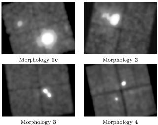
Figure 1: Examples of cluster morphology categories. The images are around 18 arcmin x 12 arcmin.

		Observer 1
			0	1	1c	2	2c	3	3c	4
Observer 2	0		10
	1			115	4	2
	1c				13		1			2
	2			4		14				1
	2c				1		1
	3							13		1
	3c
	4									10

Table 1: Morphology classes assigned to $0.1<z<0.9$ clusters by two observers (using X-ray and optical data).

The images were assigned a category by two observers, who were broadly in agreement as seen in Table 1. The few discrepancies are mainly due to small contaminating clusters which may be background fluctuations or faint undetected point sources, and cases of uncertainty over the degree of disturbance. The morphologies of Observer 1 (the first author) were adopted as they are slightly more conservative.

The optical data (from the NED) for the cluster fields were used to check for optically detected clusters in or near to the field of view (within 15′from the cluster centre). Three fields were moved from morphology class 1 to 1c as they contained optically confirmed clusters at a significantly different redshifts from the main cluster. The images were compared to the NED to check that the detected peak in the X-ray emission corresponded to the location of the galaxy cluster as given in the NED; clusters were accepted if the centre of the X-ray emission was within $3\arcmin$ of the NED object. Two cluster observations were removed as their optical position was $>3\arcmin$ from the observed X-ray peak, and therefore the optical redshift may not apply to the X-ray detected cluster. For clusters that had more than one redshift measurement in the NED the cluster redshift was accepted if $\delta z/z<0.1$. Otherwise the literature was examined in detail to determine the most accurate redshift – these clusters are flagged in Table LABEL:Cluster_tables. In addition one bright cluster has a slightly revised redshift due to an iron emission line in the X-ray spectrum, as described in Section 3.2.3.

3.2.2 The final cluster sample

The 192 cluster fields were split into samples depending on their properties. The final cluster sample contains only uncontaminated confirmed clusters to ensure that the analysis is not affected by additional clusters in or near the field of view, which could also contain AGN and may contribute to the lensing of background AGN (see Section 5.3, although this is likely to be minimal in most cases). The final sample therefore consists of the 148 observations with morphology class 1, 2 or 3 and $0.1<z<0.9$.

The twenty weakly contaminated cluster fields (1c, 2c and 3c) were included in a second sample, as the fields may still be of interest. The ten fields which clearly contained a second cluster (type 4) were rejected from the rest of the analysis.

The fourteen $z>0.9$ cluster observations with secure redshifts were placed in a third sample, regardless of the reality or extent of their emission, as at this redshift range almost all of the observed clusters are centred on active galaxies, and often the extended emission may be too faint to detect or be contaminated by AGN jets Some of these objects are better classified as proto-clusters, so they are analysed separately from the rest of the sample.

The final cluster fields, split into the above categories, are described in Table LABEL:Cluster_tables.

3.2.3 Cluster luminosities and temperatures

To compare clusters at different redshifts, luminosities need to be found in the same rest-frame band for each cluster. A spectrum was extracted from the level 2 data for each cluster and fit with a thermal model, which was then evaluated in the given band. The following analysis was applied to all cluster observations, but is only truly valid for clusters with morphology classes 1–3 as listed in Table LABEL:Cluster_tables.

Spectra were extracted from the 0.5–8 keV band data (to simplify the data reduction) from circular apertures centred on the cluster centre. The chosen aperture included $\sim 99.5$ per cent of the cluster counts, and the background spectrum was taken from an annulus with radii of 1.1 and 1.49 times the cluster radius. Point source regions were subtracted and the regions containing the brightest point sources were enlarged if necessary, to ensure that they did not contaminate the cluster emission. Areas of bad or no exposure were also removed. Response functions were calculated for the central region of the cluster aperture, rather than finding a weighted response over the full aperture, due to the time required for the latter. Tests on three clusters found that the difference in flux for a single central response file compared to that for the full region was $<2$ per cent, which is negligible compared to the errors in the model.

Spectra were fitted using an absorbed Raymond–Smith model (Raymond & Smith, 1977) in XSPEC v11.3.1, binned to a minimum of 25 counts per energy interval. The galactic neutral hydrogen density was fixed at the local values (Dickey & Lockman, 1990), and the redshift fixed to the value in Table LABEL:Cluster_tables. For clusters with more than one observation the multiple spectra were fit simultaneously. The model errors are underestimated as they do not take into account errors due to taking the calibration of the central pixel only. To get a better measure of the accuracy of the luminosities, the spectra of clusters which were observed twice were fitted individually, and the difference between the luminosities were found to be less than 0.1 dex at all fluxes. The observed luminosities of the clusters using this method are given in Table LABEL:Cluster_tables. These generally match the Chandra luminosities in the literature (e.g. Ebeling et al. 2007) to within 10 per cent.

3.3 Blank fields

It is necessary to have a control sample of blank fields in order to calculate the expected distribution of point sources in each cluster observation due to foreground and background objects (which will be referred to as ‘background sources’, although they may in fact be in the foreground). To avoid biases due to large scale structure and statistical variance due to low counts it is desirable to have as large a sample as possible of blank fields.

Many X-ray surveys of ‘blank’ fields have been conducted in order to study the general X-ray source population. Some of these observations were selected from the archive, and reduced with the pipeline to ensure consistent data reduction. Fields that contained galaxy clusters which were discovered independently of the blank field observation were removed, but fields with serendipitous cluster detections were retained. Individual pointings were selected so as to maximise the sky area and match the depth of the cluster observations.

In addition to the ‘true’ blank fields, observations of high-redshift ($z>2$) quasars or radio galaxies were also used. These were added to increase the sample size, and hence reduce the errors due to low source counts (particularly at high fluxes). In addition, all of the blank field observations used the ACIS-I detector, so observations using ACIS-S were required to test for differences due to the detector. The fields all have observation times $>10$ksec and redshifts in the NED. In most of these fields the QSO is visible at the aim-point and it is possible that there are extra sources at the redshift of the QSO due to either clustering or lensing (these will be rare as the observations are shallow and the target QSOs very distant). In all images a circle of radius $25\arcsec$ was removed from around the aim point, as this radius excludes all other objects identified in NED at the QSO redshifts (with the exception of one field, which was rejected). These regions were excluded from the analysis using the masks described in Section 5.1. One field had a further region removed due to a rare serendipitous detection of a nearby galaxy with resolved point sources.

Once the data were reduced, the blank field number counts were checked to ensure that including the high redshift QSO fields does not bias the background (as explained in the Appendix). The final sample of blank fields consists of 22 true blank fields and 22 QSO fields, which are listed in Table 3.

4 Point source detection and properties

4.1 Source detection

Images were made using unbinned data and exposure maps (in s^-1cm^-2) were made assuming the sources have a photon index of $\Gamma=1.7$, typical of unobscured AGN at the sample flux limits (see for example figure 3 of Tozzi et al., 2001). Tests on a few images showed that changing the spectral index to other realistic values does not significantly change the sources detected or their significances. Sources were detected using the wavdetect package (Freeman et al., 2002), with wavelet scales of 1,2,4,8 and 16 pixels and a significance threshold of $10^{-6}$. Tests using different wavelet scales suggest that $\ll 1$ per cent of sources are close enough to be missed by using these scales, but would be detected using scales separated by $\sqrt{2}$. The source list output from wavdetect was examined by eye to remove detections of the extended cluster emission. A montecarlo simulation of the source detection (Appendix A.1) shows that very few sources are missed by wavdetect, even accounting for the rapidly varying background in regions near the cluster centres.

Many clusters and blank fields were observed more than once, and where possible in these cases data from up to three observations were merged before the sources were detected, to give far deeper images and maximise the number of sources. Images were only merged if the same detector (ACIS-I or ACIS-S) was used. The process is similar to that for single observations with the following additions:–

The astrometry of the images was adjusted using the align_evt routine as, even after correcting the aspect files, small offsets often exist between images. Images were matched using sources detected in the central 4 arcmin of each image, where the PSF is smallest. Individual images were made, and exposure maps created for each observation. A combined image and combined exposure map were computed.

wavdetect determines whether a source is real based on the source extent and the size of the PSF, which is complex for merged images with different aim points. In this case the combined PSF size at each point was calculated by combining the PSF sizes of the individual images, weighted by their exposure map, and calculating the 3-sigma encircled energy size of the resulting source. These PSF sizes were input into wrecon in order to give detections and sizes that are comparable to the standard wavdetect results for single images.

As an illustration of this technique, Figure 2 shows the sources detected in a combined image of MACS J1149+22. The combined exposure map and expected PSF distribution are also shown.

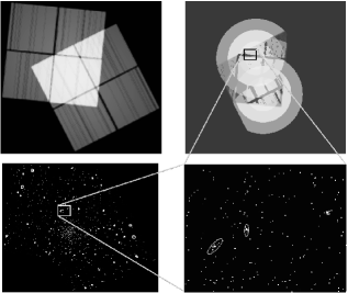
Figure 2: Source detection inputs and outputs for MACS J1149+22. The top panel shows the exposure map (left, higher exposure is white) and calculated expected PSF size distribution (right, smaller PSF is whiter) for this observation. The lower panel shows the sources detected on the combined image, using these inputs, and a enlarged portion of the image, covering an area where the expected PSF size varies rapidly. The full image is $\sim$24 arcmin across, and the pixel size is $\sim$0.5 arcsec. It is clear that the input PSF size distribution, combined with the detection power of wavdetect, accurately finds the true source centre and extent. Some detected sources could be background fluctuations, but these are later removed as described in Section 4.

4.2 Source properties

It is important to determine the source properties very accurately, as only a few percent of the detected sources are likely to be cluster sources. The observations have a wide range of exposure times, and the source sizes also change with off-axis angle, and small errors in the determination of the source properties could therefore wipe out any signal from the cluster sources, or introduce biases with, for example, redshift or exposure time.

Because of the need for high accuracy the reality and properties of the wavdetect detected sources were re-determined using more stringent criteria. This is also necessary in order to create an accurate model of detection probability, taking into account the effect of the variable background in cluster fields, as described in Section 5. wavdetect outputs were used to determine source positions and sizes, but other properties of the sources, such as counts and significance, were re-calculated. The positions and properties of some of the significant sources detected in one field are listed in Table 4, which also contains the web address of the full source list for all cluster fields.

In order to maximise the signal-to-noise for individual sources, the wavdetect source sizes were used to determine a circular aperture size for each source (as the current Chandra PSF models are only measured at a few radii). The aperture had radius $1.2\times r_{\rm max}$, where $r_{\rm max}$ is the semi-major axis of the wavdetect 3-sigma ellipse. Extensive testing showed that this radius of aperture maximised the signal-to-noise for the sample whilst minimising the missed source counts.

In deep X-ray images many sources either overlap with other sources or with areas of bad exposure such as chip gaps. Pixels in the source aperture were rejected if they were within the aperture of another source, or had exposure below 10 percent of the median value for the source. These pixels were replaced by their reflection on the opposite side of the aperture if possible, or otherwise with other pixels from the same radius. Around 3 per cent of the sources detected required some degree of correction, and for $<0.5$ per cent of sources the correction is only accurate to within a factor of $\sim$2 due to the large correction area.

For each source the mean background count rate per pixel was calculated in an annulus of area 10000 pixels, with an inner radius of $1.5\times r_{\rm max}$. Any pixels in this area within $1.5\times r_{\rm max,i}$ of a nearby source, i, or with exposure less than 10 percent of the median, were rejected. Because of the large variations in the PSF, this method works far better than an annulus scaled with aperture size and the effect of highly varying background, such as around clusters, on the source flux was found to be negligible.

The source counts are given by

$${\rm Counts}=C_{A}-\rm{Bkg}$$ (1)

$${\rm Bkg}=C_{B}\frac{N_{A}}{N_{B}}\frac{E_{A}}{E_{B}}$$ (2)

where $C$ is the total counts in a region. $E$ is the mean exposure map value of good pixels, and $N$ the number of good pixels. Subscripts $A$ and $B$ refer to the source aperture and background region respectively. $C_{B}$ is scaled by the ratio of the exposures as in $\sim 18$ per cent of sources the mean background and aperture exposure differ by over 10 percent.

Throughout the calculations the Gehrels (Gehrels, 1986) approximation $G(C)=1+\sqrt{0.75+C}$ is used to approximate both the Poissonian 1-sigma upper and lower limit.

The error on the counts is given by

$$\sigma_{\rm Counts}^{2}=\left(G(C_{A})\right)^{2}+\left(\sigma_{\rm Bkg}\right)^{2}$$ (3)

where the error on the calculated background counts in the annulus, $\sigma_{\rm Bkg}$, is

$$\sigma_{\rm Bkg}^{2}=\left(G(C_{B})\frac{N_{A}}{N_{B}}\frac{E_{A}}{E_{B}}\right)^{2}+\left(G\left(C_{B}\frac{N_{A}}{N_{B}}\frac{E_{A}}{E_{B}}\right)\right)^{2}$$ (4)

which is the combination of the error on the estimation of the background count rate, and the error on applying this (low) background value to the aperture.

The source signal-to-noise ratio (SNR) is then

$$SNR={\rm Counts}/\sigma_{\rm Counts}$$ (5)

and the significance, SIG (following Johnson et al. (2003)) is defined as

$$C_{A}={\rm Bkg}+{\rm SIG}\times\sigma_{\rm Bkg}\\$$ (6)

so that

$${\rm SIG}={\rm Counts}/\sigma_{\rm Bkg}.$$ (7)

A cut of $SIG>3$ was applied to construct a catalogue of real sources. A significance of above 3 means that the source is not a background fluctuation with above a 3-sigma probability. The correlation between $SIG$ and the SNR is very good, with a significance cut of 3 corresponding to a SNR of around 1.5. This cut is more conservative than the wavdetect significance parameter, and produces a more robust source list. On average it reduces the wavdetect source list by around 18 per cent.

To calculate fluxes (in erg cm^-2 s^-1, for the 0.5-8 keV band) the exposure map value at each pixel (in cm² s) was combined with the counts;

$${\rm Flux}=\frac{1}{k}\times\left(\sum_{i\in A}\frac{C_{i}}{E_{i}}-\frac{N_{A}}{N_{B}}\frac{E_{A}}{E_{B}}\sum_{i\in B}\frac{C_{i}}{E_{i}}\right)$$ (8)

where the summation over $i$ is over the individual pixels in a region. $k$ is the conversion from counts to ergs assuming the source has a spectrum with $F_{\nu}\propto\nu^{-1.7}$ between 0.5 and 8 keV, and energy dependent absorption by galactic hydrogen following Morrison & McCammon (1983) with column density from Dickey & Lockman (1990).

The flux missed by choosing a smaller aperture is $\sim 1$ per cent for the brightest sources and $\sim 4$ per cent for the faintest, depending on the source counts. This small correction factor was applied to the source fluxes to eliminate errors in the full population caused by differences in exposure times. Luminosities were calculated in the 0.5 – 8 keV emission band assuming a $F_{\nu}\propto\nu^{-1.7}$ spectrum.

5 Predicted source distributions

To interpret the number counts of point sources in each image an accurate model of each observation is required to determine the number of sources expected if there were no AGN in the cluster. This model requires the minimum flux detectable at each pixel and the number of blank field sources as a function of flux. The changes in sensitivity are particularly important in the cluster fields as the extended cluster emission may obscure faint central sources. The minimum flux model is described below. Section 5.2 describes the calculation of the expected number of sources for each observation, and Section 5.3 explains the correction of this prediction due to gravitational lensing by the cluster.

5.1 Modelling the sensitivity of each observation

A flux limit map was computed following the method of Johnson et al. (2003). From equation 7, the counts for a source centred at pixel i and detected at the minimum significance of 3 is $C_{min,i}=3\sigma_{\rm Bkg,i}$, which combined with equation 4 and the conversion to flux used in equation 8 gives a minimum flux detectable with significance $>3$ at pixel i of

$$S_{\rm min,i} = \frac{C_{\rm min,i}}{E_{i}k}$$ (9)

$$= \frac{3}{E_{i}k}\left(\left(G\left(R_{B,i}N_{B,i}\right)\frac{N_{A,i}}{N_{B,i}}\right)^{2}+\left(G(R_{B,i}N_{A,i})\right)^{2}\right)^{1/2}$$ (10)

where $S_{\rm min,i}$ is the minimum flux detectable with significance $>3$ at pixel i. Subscript A indicates values for the predicted source and B the predicted background, and R is the rate in counts pixel^-1sec^-1. The inputs for the prediction are then the exposure $E_{i}$, source size $N_{A,i}$ and background count rate $R_{B,i}$ at each point on the image.

The exposure is simply the sum of the individual exposure maps described in Section 4.1. There are regions where the gradient in exposure will make source detection difficult, and these are masked out later as described below. The errors in the exposure map should be small and are not easily calculable. As they will affect both the blank fields and the cluster fields in the same way they can be neglected here.

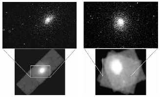
Figure 3: Background images for two cluster observations, Abell 1068 (left) and RX J1720+26 (right). The top panel shows the the central region of the images, with sources removed and the source regions marked by ellipses. The bottom panel shows the full smoothed background images (with a square root scale).

For each observation the background rate, including the diffuse cluster emission, was calculated by replacing the point sources with local background and smoothing the image with a gaussian kernel of radius 40 pixels. Figure 3 shows an example of the background images produced. To find the error on the background it is easiest to assume that the smoothed background rate is given by the average of the counts in a circle, rather than calculating the errors on the true gaussian convolved image. In other words, $R_{B,i}\approx\sum_{j\in{\rm Area}}C_{j}/{\rm Area}$ where the area is a circle of radius 40 pixels centred on i. This gives a simple equation for the error – $\sigma_{R_{B,i}}\approx\sqrt{\frac{R_{B,i}}{\pi 40^{2}}}$. To test the model background, the background rate for each detected source (using aperture photometry) was compared to that from the smoothed images at the same position. The model background accurately reproduces the calculated background for the detected sources (with SIG $>3$), with no systematic offset.

The expected source size distribution was calculated using the apertures for the detected sources from 8 representitive blank fields, and checked against the detected source sizes in all fields. Apertures derived from the wavdetect output were used instead of the given PSF size as this is how the source properties were determined. The radial distribution of aperture sizes is shown in Figure 4, which also shows the chosen model radial source size distribution. This model was determined from the data for significant, low flux sources ($S<0.25\times 10^{-14}$ erg cm^-2s^-1) which are at the detection limit of these observations. The aperture size was found to jump at radii of 480, 750 and 1010 pixels, due to the behaviour of the PSF combined with the wavelet scales chosen (this is illustrated by the fact that the brighter sources, marked by dots in Figure 4, are far closer to a constant slope, as they are affected less by the wavelet scales and trace the true change in PSF). The aperture size was modelled between each jump with a best-fit quadratic, and the 1-sigma error was determined by the distribution of sources around this fit. Above a radius of 1010 pixels the aperture size jumps considerably so this area was removed from the calculation.

Figure 4: Source size as a function of distance from the optical axis (four representitive blank fields are shown to avoid overcrowding). The mean size and 1$\sigma$ errors ware calculated for the faint sources. This is then the expected source size for sources near the flux limit at each pixel.

Again, comparison with the actual source sizes shows that this model is accurate to within the errors and has no systematic error. There were no significant differences between source sizes in the ACIS-I and ACIS-S chips. For multiple observations the source size distribution was calculated for each observation, then combined weighted by exposure map.

A mask was constructed to restrict the area to regions where the model is accurate. This removes the effects of chip gaps, chip edges and errors in the modelling. Edge effects, especially due to the background smoothing, affect areas within 60 pixels of the image edge, and 40 pixels of chip gaps, so these areas were removed. For merged images, $i$, the ‘chip boundary’ area was included if $E({\rm max})_{i}<0.5\times\Sigma_{j=good}E({\rm max})_{j}$, where $E$(max) is the on-axis exposure of an image and the sum is over all images, $j$, with good exposure in the ‘chip boundary’ area. As described in Section 5.1, regions where the model source size is greater than 700 pixels were also removed.

The final flux limit model for the two example fields is shown in Figure 5, where all cuts and masks have been applied. To check the flux limit model the fluxes of all detected sources were compared to the minimum flux detectable at the source position. Almost all ($>97$ per cent) of sources are brighter than the flux limit at their position. Those that are slightly fainter than the corresponding flux limit have large errors on their flux, so that $\ll 1$ per cent of sources are over $1\sigma$ fainter than the calculated flux limit at their position.

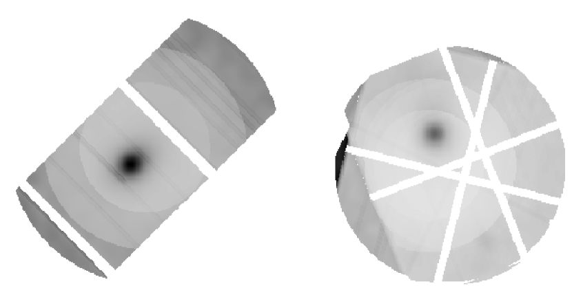
Figure 5: The final flux limit model for Abell 1068 (left) and RX J1720+26 (right). Light areas are the most sensitive and have the lowest limiting flux (1.7 and 1.2 $\times 10^{-15}$erg cm^-2 s^-1 respectively), and dark grey are the least sensitive (7.5 and 1.1 $\times 10^{-14}$erg cm^-2 s^-1). The PSF size, exposure map and cluster background all clearly affect the final limiting flux distribution.

Figure 6: The sky area sensitive to sources of flux $>S$ for one field. when no errors are applied to $S_{\rm min}$ is shown by the dotted line and 100 examples of when random errors are applied by the solid lines. The variation in the solid lines is negligible compared to the error on the number of sources.

The combined effect of the errors on $S_{{\rm min},i}$, summed over the image, is not straightforward to calculate. Random errors were added to the calculation for each pixel, and the sky area at each flux re-calculated. As the errors on the background level are correlated between pixels, the error in each 80 $\times$ 80 pixel square were changed by the same (randomly selected) number of sigma. Changing the size of this region did not change the results. The error in calculating the flux conversion factor, k, was not included as this will affect each field in the same way. Figure 6 shows the effect of these errors on one field. The sky area without errors has quite steep jumps due to the sudden changes in the model PSF (due to the wavelet scales), but applying random errors to the flux limit at each pixel smooths this distribution.

5.2 Log N($>$S) – Log S and radial distributions

The number of sources brighter than a given flux is calculated for each field, or for a combination of fields, to produce a plot of Log N($>$S) against Log S, using

$${\rm LogN}(>S_{0})=\sum_{S>S_{0}}\frac{i_{S}}{A_{S}}$$ (11)

where N($>$S₀) is the number of sources brighter than S₀, i is the number of sources of flux S, and A the total sky area available to detect a source of flux S.

The errors are dominated by the number of sources detected, so once the errors have been added to individual pixels (Figure 6), the error on the sky area can be neglected. The error on the total number of sources was used for the brightest sources, where the sky area is constant, such that;

$$\sigma_{{\rm N}(>S_{0})}=\frac{\sigma(i_{S>S_{0}})}{A}$$ (12)

for $A>0.99\times A_{max}$. When the sky area starts to decrease (at lower flux), $\sqrt{i}$ errors are used as they are able to take account of the weighting by sky area; at these fluxes the number of sources is relatively large ($i\mathrel{\hbox{\hbox to0.0pt{\hbox{\lower 4.0pt\hbox{$\sim$}}\hss}\hbox{$>$}}}$10) and the difference between Gehrels and $\sqrt{i}$ approximations becomes minimal. The error is then given by

$$\sigma_{{\rm N}(>S_{0}})=\sqrt{\sum_{S>S_{0}}\frac{i_{S}}{A_{S}^{2}}}$$ (13)

It is worth noting here the effect of the Eddington bias (Eddington, 1913), whereby random flux errors can increase the measured source counts above a chosen flux level. Manners (2002) show that the net effect for one field is $\sim 1$ per cent extra sources above $1.1\times 10^{-15}$ erg cm^-2 sec^-1. Since this is a small effect and will affect the cluster and blank field samples in the same way, it is not accounted for in the analysis.

For each field, in addition to the Log N($>$S) – Log S distribution, the radial distribution of sources was found and compared to the radial prediction assuming no cluster sources. This was calculated using the blank field Log N($>$S) – Log S and the $S_{\rm min}$ map. Errors on the predicted radial distribution were found by applying the Log N($>$S) – Log S distribution with 1$\sigma$ errors to the $S_{\rm min}$ map. The predicted and actual radial distributions were calculated from the X-ray cluster centre, or from the aim-point if no cluster was visible.

As a check of the pipeline method the radial and Log N($>$S) – Log S distributions were calculated for the 44 blank fields, as described in Appendix A.3. The pipeline prediction well reproduces the actual distribution of sources in the blank fields. In addition, checks were made for differences between the two ACIS detectors on Chandra, as described in Appendix A.4

5.3 Corrections for gravitational lensing

The effect of gravitational lensing of X-ray sources by the galaxy cluster is small, but is expected to be significant over many fields. As discussed by Refregier & Loeb (1997), after lensing the flux of each source is increased by a factor $\mu_{\theta}$, where $\theta$ is the angular distance from the cluster centre, and the number density is decreased by the same factor due to a decrease in the apparent sky area of the image. Whether this results in a net increase or decrease in sources at a given flux depends on the slope of the Log N($>S$) - Log S distribution. In moderately deep cluster observations the slope of the number counts is shallow, resulting in a deficit of sources in a lensed field compared to a blank field.

Johnson et al. (2003) estimate an expected deficit of X-ray sources of $\sim 10$ per cent in the central 0.5 Mpc of MS1054-0321 (z=0.83). This is insignificant for a single field but the cumulative effect over many fields may affect the sample. In addition, as the effect of lensing on the number counts is more significant for bright, moderate redshift clusters, gravitational lensing could bias the results.

To calculate exactly the difference between the cluster and blank fields that is due to gravitational lensing requires detailed knowledge of the dark matter distribution in the cluster. As this study is investigating a statistical excess of sources in a large number of fields, exact determination of the lensing is unnecessary (and unfeasible). Instead, the radial loss or gain of sources in each image due to the cluster is estimated using a simplified model of gravitational lensing, with the only inputs being the X-ray luminosity, position in the image and redshift of the cluster, an assumed background distribution of X-ray sources and the sensitivity distribution of the observation.

For an NFW mass profile (Navarro, Frenk & White, 1997) $\mu_{\theta}$ is only dependent on a characteristic radius and the cluster mass, as shown in Appendix A of Myers et al. (2003), using formulae and data from Maoz et al. (1997), Bartelmann (1996) and Navarro et al. (1997). Maoz et al. (1997) also show that the characteristic radius can be approximated by a function of the cluster mass. This in turn can be estimated by using the redshift dependent cluster mass - luminosity relation in equation 15 of Maughan et al. (2006). The cluster X-ray luminosities and redshifts (see Sections 3.2.1 and 3.2.3) can therefore be used to calculate the distribution of $\mu_{\theta}$ for each field. Although this calculation relies on a number of empirical relations, this will not introduce large errors as discussed below.

Three models of the X-ray background are used, as described below. They are all calculated for rest-frame 2–8 keV (hard band) sources which, where the lensing from clusters will be strongest, corresponds to observed 1–4 keV sources. The lensing factor calculated in this section is fractional, so only the shape and relative normalisation matter. It is therefore assumed that the population of hard sources in the model shows the same distribution and redshift evolution as the sources in the cluster image.

Two of the models use the Barger et al. (2001) X-ray luminosity function from $0.1<z<1.2$, but extend it to z=5. The first reduces the density by a factor of $z^{3}$ at high redshifts, which is a reasonable fit to the sources with confirmed redshifts and is therefore a lower limit. The second model scales the space density of sources such that the energy density per comoving volume remains flat at $z>1$. This is the maximum value allowed by the Barger et al. (2001) data, so is an upper limit. The third model adopted here is a luminosity dependent density evolution (LDDE) model, with best fit parameters from Ueda et al. (2003), which is the best fit to the hard X-ray luminosity function from the ChaMP survey (see Green et al. (2004) and Silverman et al. (2008) for details). The three model luminosity functions are calculated from z=0 to z=5, in redshift steps of 0.1. The lower end is important as a lot of sources will not be lensed, and these will reduce any fractional deficit due to lensing. The luminosity functions at each redshift are re-normalised to represent the sky volume visible in an image of 1 deg², rather than per cubic Mpc.

The effect of lensing on the model background source distribution is calculated as a function of cluster-centric distance, cluster redshift and cluster X-ray luminosity for each field. The lensed luminosity functions (boosted luminosities and lower space densities) of the non-cluster sources were found for redshifts 0 - 5 in steps of 0.1 and were converted to flux distributions in the observed band and summed over all redshifts. The resulting lensed Log N($<S$) – Log S distributions were compared to the unlensed distribution, and the flux limit at each point in the image, to calculate the fractional change in sources detected at each pixel. This correction was applied up to 300$\arcsec$ from the cluster centre, and gives a maximum correction per field of $\sim 1$ source.

The three models for the X-ray background distribution did not give significantly different results (far smaller than the errors on the source distribution) so only the LDDE model was used, which gives results between the two extreme models taken from the Barger et al. (2001) data. The largest source of error in this model is if there is a systematic miscalculation of the cluster properties, but this is still a small source of error overall. For example if the cluster mass is assumed to be systematically out by 30 per cent for all clusters then this would add the equivalent of 1.5 percent to the error bar at 1 Mpc. Random errors in the cluster properties due to scatter in the cluster scaling relations will generally cancel out over a large sample.

When the correction for gravitational lensing is applied, the total number of non-cluster sources predicted in an average field decreases. The prediction for the central 3 Mpc of the 148 good cluster fields is found to decrease by 0.7 per cent, which is around 0.27 sources per field on average. The calculated number of sources in the cluster, which is the number of detected sources minus the prediction, therefore increases by the same number. This is shown in Section 6.2, where the excess sources per cluster field before and after the lensing correction are compared. The number of predicted sources brighter than $10^{-14}$ erg cm^-2sec^-1 decreases by 0.6 per cent, which is 0.06 sources per field. The lensing correction is small, typically $<0.5\sigma$, but it is not insignificant as the correction is predominantly in the central regions. All statistics and plots presented in the remainder of this paper use the lensing correction, but none of the results are significantly altered if the lensing correction is ignored.

6 Results

6.1 Excess sources in cluster fields

Figure 7: The excess number of sources per field, compared to the prediction, for 44 blank fields and 148 uncontaminated cluster fields with $0.1<z<0.9$. The mean for the cluster fields is $1.46\pm 0.32$, compared to $0.47\pm 0.61$ for the blank fields.

The number of cluster sources in each field was estimated by subtracting the predicted number of sources (Section 5) from the actual number of well-detected sources (Section 4), to get the excess sources in each field. The results presented in Figure 7 show the excess sources within 1 Mpc of each cluster centre, which is the maximum radius observed for the lowest redshift clusters. The resulting histogram shows that cluster fields have a wide spread of calculated excess sources, including negative values, but that the average excess is clearly non-zero. For the blank fields, with assigned redshifts randomly chosen from the redshift distribution of cluster fields, the excess sources within 1 Mpc of each field are consistent with zero. Figure 7 shows that the galaxy clusters have, on average, around 1.5 sources each within a projected distance of 1 Mpc. This value is an average over clusters of different redshifts and luminosities, and observations of different exposure time; the dependence of number of cluster X-ray sources on these variables will be analysed in the next paper in this series.

The Log N($>S$) – Log S distribution was plotted for the blank fields and the 148 uncontaminated cluster fields with $0.1<z<0.9$. Figure 8 shows that the cluster fields have a $\sim 2\sigma$ excess at fluxes of $>10^{-13.7}$ erg cm^-2sec^-1. An excess of $\sim 1\sigma$ is seen at fainter fluxes. These are not strongly dependent on the lensing correction, which changes the results by a maximum of $0.2\sigma$. A Kolmogorov–Smirnov (K–S) test on the sources brighter than $>10^{-13.7}$ erg cm^-2sec^-1 shows that the cluster and blank field populations differ at the 96 per cent level.

The most significant excess in the Log N($>S$) – Log S distribution is found at bright fluxes, but this is partly due to the lower number of bright background sources. In fact only half of the excess sources within 1 Mpc have flux $>10^{-14}$ erg cm^-2sec^-1 (a mean of 0.76 $\pm$0.18 per field). Sources brighter than this flux are quite likely to be AGN, as this corresponds to a (k-corrected) luminosity of $>2.5\times 10^{41}$ erg sec^-1 in all clusters, and $>10^{42}$ erg sec^-1 in over 80 per cent of the sample. In clusters with $z<0.2$ sources with luminosity $<10^{41}$ erg sec^-1 can be detected, which are far less likely to be AGN, but the majority of sources have either flux $\gg 10^{-14}$ erg cm^-2sec^-1 or are in higher redshift clusters and so are likely to be AGN.

Figure 8: The combined Log N($>S$) – Log S distribution within 1 Mpc of the cluster centres for the 44 blank fields and 148 uncontaminated cluster fields with $0.1<z<0.9$.

6.2 Radial distribution of cluster sources

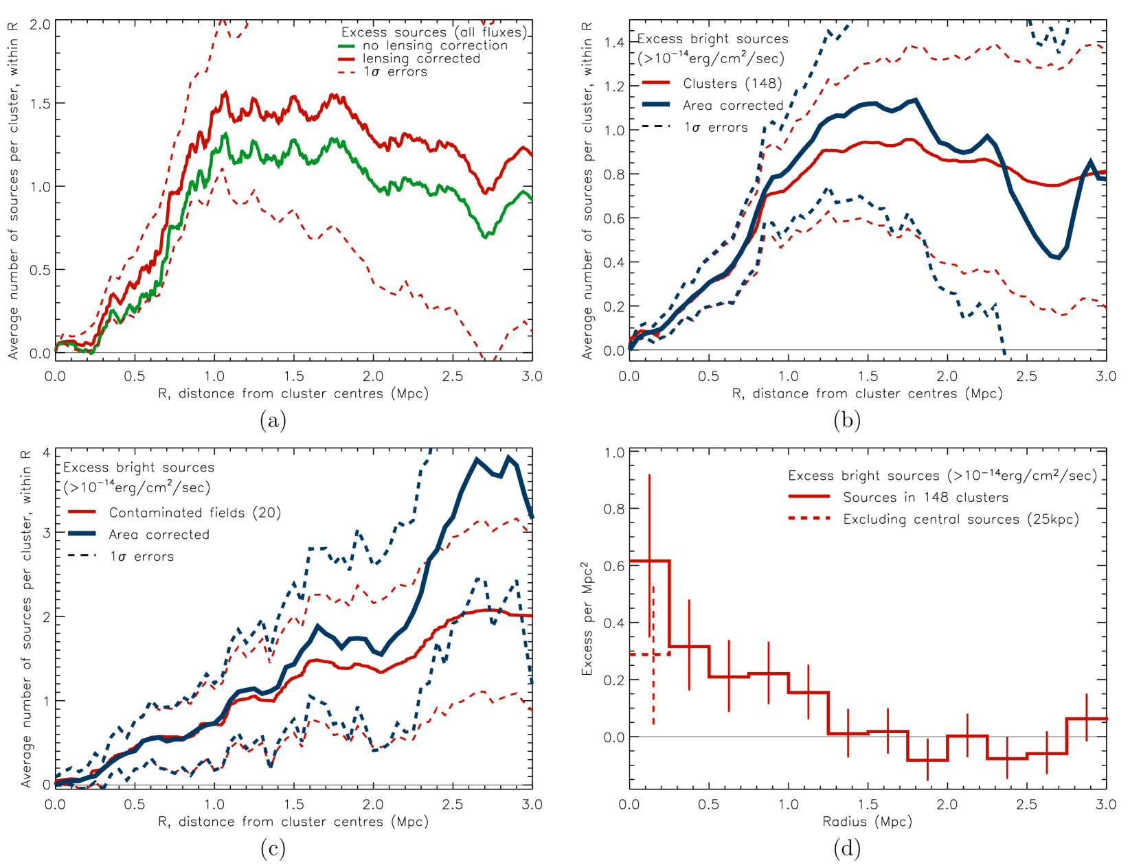
Figure 9: The number of excess sources per field within a given radius (total detected sources minus the predicted background and foreground sources), and 1$\sigma$ errors, for (a) 148 uncontaminated cluster fields with $0.1<z<0.9$ corrected for gravitational lensing (red line and error bars), and without the lensing correction (green line). All sources are shown, and the cluster fieldss have a significant excess of sources within 1 Mpc; (b) the same 148 clusters (thin red line), but restricted to sources with flux $>10^{-14}$ erg cm^-2sec^-1, which are detectable in almost all regions of all cluster images. The thick blue ‘area corrected’ line shows the same distribution corrected for the missing area at each radius, due to low sensitivity or gaps in the detector. (The ‘area corrected’ distribution has higher errors and a more variable line at high radius, as a lower fraction of the total area is covered in these regions.); (c) 20 contaminated cluster fields i.e. those with another probable cluster in the field of view. As in plot (b), the thin red line shows sources $>10^{-14}$ erg cm^-2sec^-1 and the thick blue ‘area corrected’ line includes a correction for the missing area at high radius. The significant excess of sources at $1-3$ Mpc, when corrected for the missing area, shows that these fields contain sources which are not associated with the main cluster, and therefore should not be included in this analysis. (d) The number density of excess sources in each 0.5 Mpc bin, for the same 148 uncontaminated cluster fields. The dashed line shows the first bin excluding sources within 25 kpc of the cluster centres.

The radial distribution of all excess sources in the cluster fields is shown in Figure 9(a). The cluster fields clearly have an excess of around 1.5 sources per cluster, whereas the blank fields have no statistical excess. Although this excess is of low significance at 3 Mpc, all of the excess sources lie within 1 Mpc from the cluster centres and within this radius the significance of the excess is $>3\sigma$, with a maximum significance of $>3.5\sigma$ at 0.85 Mpc. There are no excess sources at $\mathrel{\hbox{\hbox to0.0pt{\hbox{\lower 4.0pt\hbox{$\sim$}}\hss}\hbox{$>$}}}1$ Mpc despite the fact that two thirds of all detected sources are beyond this radius. Figure 9(a) also shows the radial distribution without correction for gravitational lensing. As explained in Section 5.3, the number of sources per cluster field is lower but still highly significant.

It is possible that the lack of sources at $>1$ Mpc is due to the fall off in sensitivity with radius. To check for this the radial distribution of sources brighter than $10^{-14}$ erg cm^-2 sec^-1, which can be well detected at all radii, is plotted in Figure 9(b). In addition some of the lack of sources could be due to the reduced sky area at higher radius, so the distribution for bright sources was corrected for the proportion of missing area at each increase in radius. Both distributions show that the cluster sources are still found within $\sim$1 Mpc, with a $\sim 3\sigma$ excess in this area. There is no excess above this radius, although as the errors are larger in this plot some cluster sources could lie beyond 1 Mpc. The correction for gravitational lensing for these brighter sources is not plotted as it negligible (see Section 5.3).

Figure 9(c) shows the same figure for the twenty contaminated fields, which are those which had a second region of extended X-ray emission that was not clearly associated with the cluster, or an optically detected cluster in the field. The distribution of sources is clearly different to that for the 148 uncontaminated clusters, with excess sources seen up to 3 Mpc from the cluster centres. The number of sources per cluster in the contaminated fields is similar at 1 Mpc (within the errors) but larger at higher radius. This justifies the decision not to include these clusters in the analysis, as it is very likely that they include sources associated with the contaminating clusters on the outskirts of the fields.

Figure 9(d) shows the density of sources with flux $>10^{-14}$ erg cm^-2sec^-1 as a function of radius. It is clear from this figure that a number of sources lie in the very central regions of the cluster, and are likely to be AGN in the Brightest Cluster Galaxy (BCG). Whereas the fraction of radio detected AGN in BCGs is known (Best et al., 2007) the number of X-ray detected AGN is not well defined, and detection is complicated by the extended X-ray emission. Ruderman & Ebeling find that $\sim$10 per cent of their clusters have a detected X-ray source within 250 kpc of the cD galaxy in the cluster centre.

In this sample 166 clusters have $0.1<z<1$ and no chip boundaries in the cluster centre. Twelve of these 166 clusters have X-ray sources within the central 25 kpc, defined from the centre of the X-ray emission, whereas only one would be expected randomly. One of these clusters, 3C 295, has two sources within this radius. Outside this radius there are very few additional sources compared to the background prediction. The k-corrected luminosities of these sources are listed in Table LABEL:Cluster_tables. To find the proportion of clusters hosting X-ray detected AGN it is necessary to find the detection threshold at the centre of each cluster. Neglecting the second source in 3C 295 the fraction of clusters with AGN with 0.5–8 keV k-corrected luminosity $>L_{X}$ increases from $2.4^{+1.9}_{-1.2}$ per cent at $L_{X}=10^{44}$ erg sec^-1, to $4.9^{+2.5}_{-1.7}$ per cent at $10^{43}$ erg sec^-1 and $7.5^{+4.5}_{-3.7}$ per cent at $10^{42}$ erg sec^-1. Below this luminosity most clusters are too bright to detect AGN and so the statistics are not significant.

When the central sources are excluded in Figure 9(d) the projected source density is flat or slightly falling until $\sim$1.25 Mpc, where it falls to zero. This is consistent with a random distribution in projected area, which is naively not the expected distribution of galaxies in clusters. However, the distribution of X-ray sources here is consistent with the radial distribution of cluster galaxies in Martini et al. (2007), so it may be that X-ray sources simply trace the underlying population. This will be investigated further in the next paper in this series (Gilmour et al. in prep.).

6.3 Comparison with previous studies

Most of the clusters that have been studied by other authors are also included in this sample, and in the majority of cases the results of this analysis agree with the previous results within the errors. The analyses of many small studies, and the larger studies of Martini et al. (2007), Branchesi et al. (2007) and Ruderman & Ebeling (2005), have been reproduced as far as possible and are compared below.

Comparing the number of excess sources found by the pipeline in individual clusters to previous studies, the values are in good agreement for most clusters; A2104 (Martini et al., 2002), 3c295 (Cappi et al., 2001), MS1054-03 (Johnson et al., 2003), MS0451-03 (Molnar et al., 2002), six of the clusters from Cappelluti et al. (2005) and MRC 1138-262 (Pentericci et al., 2002). For a few clusters this study produces different results in the overall number of sources to those found in Cappelluti et al. and Cappi et al., as these authors present results on a chip-by-chip basis rather than as a radial analysis. Visual inspection of these fields indicates that their conclusions are consistent with those from this survey.

Of the eight clusters studied spectroscopically by Martini et al. (2007), five are included in this study. The results agree very well (less than 1$\sigma$ difference) with the Martini et al. results, both in terms of number and radial distribution of the sources. Martini et al. find 17 sources within 1 Mpc in these five clusters, and 12 within 0.5 Mpc. This study gives 17.5 within 1 Mpc and 9.5 within 0.5 Mpc. At higher radii the errors in this study become too large to draw any conclusions for 5 fields. In both studies the AGN are predominantly found in the central regions of these 5 clusters, with twice as many sources at low radius ($<$ 0.5 Mpc) than at higher radius (0.5 - 1 Mpc). However, from Figure 9(b) it is clear that this is not the case for the full sample of 148 clusters – rather the number of sources at $<$0.5 Mpc is closer to half the value at higher radius (0.5 - 1 Mpc). The central concentration of the Martini et al. AGN is therefore not representative of clusters in general, perhaps because the Martini et al. clusters have particular properties. This will be investigated further in the next paper in this series (Gilmour et al., in prep.) when the 148 clusters are split into subsamples according to redshift and cluster properties.

Branchesi et al. (2007) performed a statistical analysis of point sources in 18 clusters, of which 15 are in this sample. They find a $1.7\sigma$ excess of bright sources within 1 Mpc ($F_{X}>10^{-14}$ erg cm^-2sec^-1 ). The 15 clusters in this paper have the same $1.7\sigma$ excess at the bright end of the Log N($>S$) – Log S distribution, which also fits with the results for the full sample in Figure 8. Branchesi et al. find 7(2) cluster(blank) sources at $<$0.5 Mpc, and 4(3) sources at 0.5–1.0 Mpc and conclude that the majority of sources are in the central 0.5 Mpc of the cluster. However, they only search to the edge of the intra-cluster emission, which gives an average search radius of 0.8 Mpc. The results for this study, correcting for missing clusters and different flux bands, agree with the Branchesi et al. values but the number of sources rises steeply beyond 0.8 Mpc, so the conclusion that the vast majority of AGN are found within 0.5 Mpc is not confirmed if larger radii are investigated. As an aside, it is worth noting that five of the fifteen fields investigated here are classed as contaminated in this study (morphology type 1c, 2c, or 4 in Table 1). In agreement with Section 6.2, a significant number of sources continue to be found in these fields up to 3 Mpc from the cluster centres.

Ruderman & Ebeling (2005) study 51 massive galaxy clusters at $0.3<z<0.7$, and conclude that the point sources lie predominantly in the central 0.5 Mpc, with a secondary excess at 2 - 3 Mpc. This is significantly different from the results shown in Figure 9(d). In this study, using the 25 clusters with published redshift, the excess in the central 0.5 Mpc is found, but the high significance (8$\sigma$) of this excess found by Ruderman & Ebeling and the secondary excess at larger radius, are not. One possible explanation of this is that Ruderman & Ebeling measure their excess from the point source density at $>4$ Mpc which, as they themselves point out, is lower than that in the control (blank) fields. If the value implied from their blank fields is applied to the cluster sample, then the secondary excess at 2–3 Mpc is no longer significant and the central excess is of lower significance, in agreement with this study. It appears that their point source density at large radii is artificially low due to not subtracting the background sources before scaling to physical radius. The density of non-cluster sources, when scaled to the cluster redshift, is dependent on the redshift, and at higher physical radius only the high redshift fields are used to calculate the point source density, leading to a lower value. As their point source list and cluster sample are not yet published it is not possible to test this further.

6.4 The brightest sources

Figure 10: The radial distribution of all sources with flux $>10^{-12.5}$ erg cm^-2sec^-1. Solid, hatched and white bars indicate confirmed cluster AGN, possible cluster AGN and background/foreground sources respectively. A random distribution, based on the available sky area, is marked by the solid line. The confirmed and possible cluster AGN are not randomly distributed in physical distance from the cluster centres. Ignoring the central four AGN, a K-S test shows that the distribution in Mpc is not random with 98.5 per cent probability.

As a further test of the validity of the conclusions the distribution of the very brightest sources, which are clearly highly luminous AGN if they are in the cluster, was investigated in detail. Sources brighter than $10^{-12.5}$ erg cm^-2sec^-1, which are easily detected over the full sample area, were compared to the NED to identify possible cluster AGN and eliminate contaminating sources. The results, shown in Figure 10, confirm that the AGN primarily lie within 1.25 Mpc from the cluster centre. The 13 AGN which could be cluster members are clustered in two groups - one at the cluster centres and a second at $\sim$1 Mpc. There is tentative evidence here that the very brightest sources lie in the outskirts of the cluster, but this will be investigated in the next paper in this series. It is clear that these sources are not foreground objects but are associated with the clusters, as they are not drawn from a random distribution with $>99.93$ per cent probability for all AGN, and 98.5 per cent if the central four AGN are excluded.

7 Conclusions

The X-ray point source population in moderately deep ($>10$ ksec) Chandra observations of 148 cluster fields and 44 blank fields were calculated and compared in order to estimate the number of X-ray sources in the galaxy clusters. The number of sources is found to be low, with 1.5 sources in a typical cluster. This result is significant to $>3\sigma$, but the actual number of sources per cluster depends on the exposure time and the redshift of the cluster. Over half of these sources have fluxes corresponding to luminosities $>10^{42}$ erg sec^-1 and are likely to be AGN. The population is not dominated by AGN in the central galaxy (BCG), as only twelve clusters have a central source, rather the sources are AGN or star-burst galaxies in normal cluster members. They are all found in the central 1 Mpc of the cluster, and are randomly distributed in projected area within this radius.

Many of the clusters covered by similar studies (e.g. Branchesi et al. 2007; Martini et al. 2007; Ruderman & Ebeling 2005) are included in this sample, and when the same clusters are compared then the results are generally in good agreement. However the conclusions drawn from these papers, which use smaller numbers of clusters, are often not borne out by this larger study. For example a higher number of sources is found in the central 0.5 Mpc than the annulus at 0.5 - 1 Mpc in all three previous studies of more than six clusters, and whilst these results can be reproduced by this study for the smaller samples, the cluster population in general has more sources in the outskirts (0.5 - 1 Mpc) of the cluster than the central 0.5 Mpc. In Appendix A.2 it is demonstrated that samples of less than five clusters suffer strongly from cosmic variance in the number of background sources, but larger samples are also affected to some extent. The question of whether the discrepancies between this study and some of the previous papers in this field is due to cluster properties or the larger sample size in this study will be investigated in the next paper in this series.

This paper describes a sample of point sources in cluster fields which can be used to investigate the number and properties of X-ray sources in galaxy clusters as a function of cluster properties and redshift, and hence increase our understanding of the links between environment and AGN. This, the first paper in the series, serves as an introduction to the sample and comparison to previous studies. Subsequent papers (Gilmour et al. in prep) will use this study to investigate in more detail the environments of cluster AGN.

Table 2: The final cluster sample, split by morphological class.

Table 2
NED Name	Obs Ids	RA	DEC	Array	Exp	$F_{x}$	$L_{x}1$	$L_{x}2$	r$\chi^{2}$	z	Ref	Excess	Centre
Morphology 1 clusters:
CL 0016+1609	520	00:18:33.6	+16:26:12.6	I	67.2	2.32	23.06	8.31	0.92	0.544	1,2	$-2.37^{+3.18}_{-1.94}$
1RXS J003539.8-122247	5010	00:25:29.7	-12:22:41.9	I	24.7	1.03	13.40	5.79	0.95	0.584	3	$-3.23^{+2.32}_{-0.87}$
ZwCl 0024.0+1652	929	00:26:35.8	+17:09:41.1	S	38.9	0.50	2.71	1.32	0.90	0.39	4	$8.92^{+5.67}_{-4.56}$
RX J0027.6+2616	3249	00:27:45.4	+26:16:22.5	I	9.9	0.83	3.51	1.35	0.96	0.367	5	$0.30^{+3.18}_{-1.94}$
CRSS J0030.5+2618	1190,1226	00:30:34.0	+26:18:09.9	S	37.1	0.26	2.36	0.94	1.02	0.50	6	$0.90^{+4.12}_{-2.96}$
ABELL 0068	3250	00:37:06.4	+09:09:29.3	I	10.0	4.18	7.61	2.87	0.91	0.255	7	$4.4^{+4.12}_{-2.96}$
ABELL 0209	522,3579	01:31:53.4	-13:36:44.1	I	19.9	6.94	8.03	3.58	0.99	0.206	7	$-5.52^{+3.19}_{-1.95}$
NSCS J015924+003024	5777	01:59:17.1	+00:30:13.3	I	19.8	0.43	2.32	1.30	1.12	0.386	8	$-2.89^{+2.94}_{-1.66}$
WARP J0216.5-1747	5760	02:16:32.5	-17:47:34.9	I	36.1	0.79	10.30	4.07	1.06	0.578	9	$5.47^{+4.42}_{-3.28}$
CL J023026.6+183622	5754	02:30:28.6	+18:36:14.7	I	67.6	0.14	3.88	1.35	1.02	0.799	10	$2.28^{+3.96}_{-2.78}$
RXC J0232.2-4420	4993	02:32:18.5	-44:20:48.2	I	18.0	6.89	16.55	7.42	1.11	0.284	11	$-1.23^{+3.40}_{-2.18}$
MACS J0242.6-2132	3266	02:42:35.9	-21:32:26.3	I	11.7	4.72	15.03	7.56	1.00	0.314	12	$2.39^{+3.78}_{-2.60}$
ABELL 0383	524,2320	02:48:03.5	-03:31:44.4	I	29.2	5.46	5.36	2.79	1.19	0.187	7	$2.3^{+5.34}_{-4.23}$
1RXS J025709.6-232549	1654	02:57:09.1	-23:26:05.2	I	19.8	1.77	15.64	6.66	0.95	0.505	3	$-1.46^{+2.93}_{-1.66}$
CL J030221.3-042329	5782	03:02:21.1	-04:23:24.5	I	10.0	2.21	8.96	4.15	0.83	0.35	10	$0.36^{+3.18}_{-1.94}$
Cl 0302+1658	525	03:05:31.6	+17:10:08.6	I	10.0	0.45	2.84	1.19	0.38	0.424	2	$-1.12^{+2.66}_{-1.32}$
1RXS J032649.5-004341	5810	03:26:50.0	-00:43:51.5	I	9.9	2.29	15.96	6.48	0.64	0.448	13	$0.50^{+2.93}_{-1.66}$
MACS J0329.7-0212	6108	03:29:41.6	-02:11:46.6	I	39.4	2.12	15.00	6.30	1.05	0.45	14	$-1.50^{+3.40}_{-2.18}$
CL J033310.2-245641	5764	03:33:10.5	-24:56:32.5	I	37.0	0.15	1.36	0.76	0.91	0.475	10	$-3.9^{+3.18}_{-1.94}$
CL J035043.9-380125	7227	03:50:40.8	-38:02:09.9	I	24.4	0.21	0.97	0.55	0.70	0.363	10	$0.17^{+3.78}_{-2.60}$
CL J035559.3-374146	5761	03:55:59.4	-37:41:45.9	I	27.6	0.32	2.73	1.46	0.98	0.473	10	$-1.91^{+3.18}_{-1.94}$
RBS 0531	3270	04:17:34.7	-11:54:35.7	I	12.0	6.33	39.05	14.67	0.98	0.44	15	$2.19^{+3.39}_{-2.18}$
RX J0439.0+0715	526,1449,3583	04:39:00.7	+07:16:05.6	I	27.0	5.19	7.66	2.86	0.95	0.23	16	$1.84^{+4.71}_{-3.58}$
RX J0439.0+0520	527	04:39:02.3	+05:20:44.0	I	9.5	3.73	4.55	2.00	0.72	0.208	16	$1.81^{+3.96}_{-2.79}$
MS 0440.5+0204	4196	04:43:09.9	+02:10:19.7	6,7	45.1	1.55	1.53	0.63	1.22	0.19	2,17	$2.7^{+6.48}_{-5.40}$
RX J0521.1-2530	5758	05:21:11.7	-25:31:12.5	I	14.9	0.01	0.33	0.33	0.09	0.581	8	$1.72^{+3.39}_{-2.18}$
BMW-HRI J052215.8-362453	5837	05:22:15.4	-36:25:04.5	I	27.6	0.17	1.43	0.67	0.70	0.472	8	$2.4^{+3.96}_{-2.78}$
RBS 0653	4994	05:28:52.8	-39:28:20.5	I	16.8	4.42	10.48	4.66	0.90	0.284	11	$4.84^{+4.43}_{-3.28}$
CL J054250.8-410005	914	05:42:49.8	-41:00:00.2	I	50.2	0.33	4.87	1.84	0.88	0.634	18	$2.79^{+3.96}_{-2.78}$
MACS J0647.7+7015	3196,3584	06:47:50.3	+70:14:54.6	I	39.0	1.68	19.07	6.33	0.83	0.584	1	$2.75^{+3.96}_{-2.78}$
ZwCl 0735.7+7421	4197	07:41:44.6	+74:14:37.3	6,7	45.3	5.77	7.81	3.92	1.38	0.216	2	$-7.48^{+4.73}_{-3.60}$
MACS J0744.9+3927	3197,3585,6111	07:44:52.7	+39:27:26.9	I	89.0	1.38	24.35	8.57	1.15	0.686	1	$3.65^{+4.28}_{-3.12}$
PKS 0745-19	508,2427	07:47:31.4	-19:17:41.7	S	36.8	57.56	14.87	4.24	1.56	0.103	19	$-2.7^{+5.92}_{-4.83}$
ZwCl 0806.5+2822	5774	08:09:41.9	+28:12:06.9	I	17.7	0.79	2.28	1.21	0.93	0.30	2	$1.32^{+3.96}_{-2.79}$
RX J0819.6+6336	2199	08:19:26.0	+63:37:24.0	S	14.5	2.98	1.10	0.60	1.11	0.119	16	$0.99^{+5.46}_{-4.36}$
RX J0820.9+0751	1647	08:21:02.0	+07:51:48.8	S	8.2	1.63	0.51	0.33	1.02	0.11	20	$1.86^{+5.11}_{-3.99}$
ABELL 0665	531,3586	08:30:58.7	+65:50:31.4	I	38.6	9.12	10.99	4.50	1.13	0.182	7,21	$4.48^{+5.78}_{-4.68}$
4C +55.16	4940	08:34:55.0	+55:34:21.2	6,7	92.0	3.59	6.35	3.29	1.44	0.242	22	$0.79^{+6.21}_{-5.12}$	43.76
2MASX J08425596+2927272	2224	08:42:55.9	+29:27:25.5	S	29.4	3.14	3.39	1.84	1.25	0.194	2	$-3.56^{+5.11}_{-3.99}$
ABELL 0697	532,4217	08:42:57.5	+36:21:56.1	I	23.6	7.30	16.61	6.50	1.10	0.282	7	$1.23^{+4.12}_{-2.96}$
RX J0850.1+3604	1659	08:50:06.7	+36:04:17.1	I	22.1	2.94	12.99	5.19	0.93	0.378	5,16	$2.68^{+4.12}_{-2.96}$
ZwCl 0848.5+3341	4205	08:51:39.0	+33:31:08.0	S	11.4	1.03	4.81	2.04	1.15	0.380	23	$-2.22^{+2.94}_{-1.66}$
MACS J0913.7+4056	509	09:13:45.4	+40:56:27.6	S	7.8	1.46	10.00	4.18	0.87	0.442	24	$0.2^{+3.18}_{-1.94}$	44.3
ABELL 0773	533,3588,5006	09:17:52.9	+51:43:39.2	I	30.4	6.57	8.54	3.87	1.03	0.217	7,5	$10.28^{+6.8}_{-4.98}$
RX J0926.6+1242	5838	09:26:36.6	+12:43:03.4	I	31.3	0.30	2.77	1.41	1.02	0.489	8	$3.92^{+4.28}_{-3.12}$
MACS J0947.2+7623	2202	09:47:13.0	+76:23:14.2	I	11.7	6.30	24.61	11.48	0.91	0.35	25	$1.15^{+3.40}_{-2.18}$	44.65
ZwCl 0947.2+1723	3274	09:49:51.8	+17:07:08.1	I	14.3	3.19	14.28	5.42	0.73	0.383	5	$3.98^{+3.96}_{-2.78}$
ZwCl 0949.6+5207	3195	09:52:49.3	+51:53:04.9	S	26.5	4.35	5.87	3.26	1.01	0.214	16	$5.88^{+5.88}_{-4.78}$
RX J0956.0+4107	5759	09:56:03.2	+41:07:13.0	I	40.0	0.28	3.79	1.81	0.98	0.587	8	$-4.2^{+2.66}_{-1.33}$
CL J095819.3+470217	5779	09:58:19.2	+47:02:03.5	I	25.1	0.25	1.40	0.82	1.06	0.39	26	$0.89^{+3.96}_{-2.79}$
ABELL 0907	535,3185,3205	09:58:21.9	-11:03:50.9	I	104.6	8.58	5.31	2.44	1.42	0.153	27	$7.60^{+7.66}_{-6.59}$
MS 1008.1-1224	926	10:10:32.3	-12:39:34.5	I	43.6	2.21	6.00	2.40	1.23	0.301	2	$3.93^{+4.97}_{-3.85}$
ZwCl 1021.0+0426	909	10:23:39.7	+04:11:09.2	I	45.8	10.14	25.66	11.40	1.00	0.291	28	$4.78^{+5.22}_{-4.10}$
ABELL 1068	1652	10:40:44.6	+39:57:10.2	S	26.7	10.63	5.41	3.22	1.50	0.138	7	$8.60^{+6.74}_{-5.66}$
RX J1008.8+0906	3252,5009	11:08:55.3	+09:05:58.5	I	34.1	1.18	8.73	3.77	0.86	0.463	23	$0.46^{+3.78}_{-2.60}$
WARP J1113.0-2615	915	11:13:05.1	-26:15:38.8	I	104.2	0.10	2.46	1.01	1.09	0.725	9	$1.9^{+4.12}_{-2.96}$
ABELL 1204	2205	11:13:20.4	+17:35:38.7	I	23.5	6.78	5.52	3.41	1.24	0.171	7,5	$1.89^{+5.57}_{-4.47}$
RX J1115.8+0129	3275	11:15:51.9	+01:29:55.6	I	14.6	4.84	18.57	7.72	0.93	0.38	29 (N1)	$0.95^{+3.40}_{-2.18}$
RX J1120.1+4318	5771	11:20:06.9	+43:18:06.5	I	19.8	0.41	6.11	3.00	0.87	0.6	30	$1.31^{+3.39}_{-2.18}$
RX J1130.9+2326	1660	11:20:57.4	+23:26:33.1	I	70.6	0.25	3.30	1.79	0.95	0.562	8	$2.5^{+4.43}_{-3.28}$
MS 1137.5+6624	536	11:40:22.3	+66:08:16.1	I	117.2	0.27	7.21	2.94	0.87	0.782	31	$-3.48^{+3.40}_{-2.19}$
ABELL 1361	2200,3369	11:43:39.7	+46:21:20.0	S	15.9	4.60	1.64	0.97	1.07	0.117	7,5	$0.8^{+5.69}_{-4.59}$
ABELL 1413	537,1661,5003	11:55:18.0	+23:24:16.2	I	94.1	16.17	8.33	3.65	1.28	0.142	7,5	$0.55^{+6.59}_{-5.50}$
ABELL 1446	4975	12:02:04.7	+58:02:12.0	S	58.2	2.87	0.77	0.44	1.11	0.103	5	$0.36^{+7.52}_{-6.46}$	41.70
CLG J1205+4429	4162	12:05:51.4	+44:29:10.8	S	29.7	0.05	0.82	0.50	1.08	0.592	32	$-3.88^{+2.94}_{-1.66}$
RXC J1206.2-0848	3277	12:06:12.4	-08:48:03.9	I	23.4	4.70	28.82	10.65	1.07	0.441	33,29	$1.41^{+3.60}_{-2.40}$
RBS 1080	5833	12:13:23.1	-26:18:07.9	6,7	9.9	0.61	1.41	0.60	0.95	0.278	34	$-1.75^{+3.40}_{-2.18}$	43.16
RX J1213.5+0253	4934	12:13:35.0	+02:53:47.9	I	18.7	0.25	1.38	0.63	0.77	0.409	8	$0.60^{+3.60}_{-2.40}$
RX J1216.3+2633	4931	12:16:19.9	+26:33:12.4	I	17.5	0.20	1.41	0.80	0.86	0.428	6	$-1.1^{+3.18}_{-1.94}$
RX J1221.4+4918	1662	12:21:26.3	+49:18:27.2	I	78.7	0.38	7.47	3.26	0.95	0.7	6	$0.41^{+3.78}_{-2.60}$
CL J122201.9+270919	5766	12:22:01.9	+27:09:32.4	I	49.0	0.18	1.54	0.85	1.08	0.472	10	$0.49^{+3.96}_{-2.79}$
BMW-HRI J122657.3+333253	5014	12:26:58.0	+33:32:47.1	I	32.6	0.86	26.81	10.23	1.04	0.89	35	$1.23^{+3.39}_{-2.18}$
ABELL 3541	1648	13:03:42.4	-24:14:45.3	S	9.7	7.78	3.35	1.80	1.28	0.128	7	$-4.45^{+3.80}_{-2.62}$
MACS J1311.0-0311	3258,6110	13:11:01.7	-03:10:38.5	I	77.8	1.11	9.92	4.79	0.95	0.49	13	$4.61^{+4.71}_{-3.57}$
ABELL 1689	7289	13:11:29.5	-01:20:29.8	I	74.9	18.52	16.40	7.10	1.42	0.183	7	$5.92^{+6.57}_{-5.48}$
RX J1320.0+7003	3278	13:20:07.9	+70:04:36.8	I	20.5	1.74	5.74	2.58	0.73	0.328	7,5	$5.42^{+4.57}_{-3.43}$
ZwCl 1332.8+5043	5772	13:34:20.1	+50:31:01.2	I	17.6	0.36	5.54	2.67	1.00	0.62	30	$3.71^{+3.78}_{-2.59}$
RX J1340.5+4017	3223	13:40:32.9	+40:17:38.7	S	46.4	0.16	0.13	0.13	1.05	0.171	36	$6.78^{+7.18}_{-6.10}$
LCDCS 0829	3592	13:47:30.8	-11:45:10.1	I	57.4	10.78	68.09	23.48	1.16	0.451	37,38	$-1.92^{+3.40}_{-2.18}$
RDCS J1350+6007	2229	13:50:48.3	+60:07:06.0	I	58.1	0.12	3.99	1.98	1.05	0.804	39	$2.70^{+4.12}_{-2.96}$
ZwCl 1358.1+6245	516	13:59:50.6	+62:31:02.9	S	52.1	2.42	8.31	3.80	1.11	0.328	2	$1.52^{+5.34}_{-4.23}$
ABELL 1835	495,496	14:01:02.0	+02:52:41.6	S	30.2	18.40	34.36	14.89	1.58	0.253	7	$-2.33^{+4.58}_{-3.44}$
3C 295	578	14:11:20.4	+52:12:10.0	S	17.9	0.87	6.92	3.43	1.21	0.46	40	$7.57^{+4.84}_{-3.71}$	43.77(N2)
NSCS J141623+444558	541	14:16:27.9	+44:46:44.5	I	30.7	0.58	3.38	1.80	1.02	0.4	6	$-2.53^{+3.40}_{-2.18}$
MACS J1423.8+2404	4195	14:23:47.9	+24:04:42.6	6,7	115.2	1.92	22.14	9.91	1.20	0.545	1	$3.73^{+5.10}_{-3.98}$
ABELL 1914	542,3593	14:26:02.0	+37:49:32.8	I	26.7	19.03	14.54	6.18	1.00	0.171	7	$5.23^{+5.78}_{-4.68}$
RBS 1460	5793	15:04:07.5	-02:48:16.1	I	38.9	25.15	32.46	13.57	1.22	0.215	41	$-1.19^{+4.72}_{-3.58}$
ABELL 2034	2204	15:10:11.8	+33:30:54.3	I	53.8	10.73	3.41	1.59	0.97	0.113	7	$3.82^{+8.49}_{-7.43}$
RX J1532.5+3021	1665	15:32:53.8	+30:20:58.6	I	9.9	5.92	22.92	11.18	1.08	0.345	16 (N3)	$1.18^{+3.40}_{-2.18}$
ABELL 2111	544	15:39:41.3	+34:25:06.7	I	10.3	3.57	5.18	2.26	1.02	0.229	7	$-1.70^{+3.40}_{-2.19}$
ABELL 2104	895	15:40:07.9	-03:18:17.5	S	49.0	8.94	5.42	1.80	1.72	0.153	7,42	$12.18^{+7.41}_{-6.34}$
WARP J1552.2+2013	3214	15:52:12.8	+20:13:39.9	S	14.9	0.23	0.11	0.08	1.06	0.136	6	$-3.30^{+4.86}_{-3.74}$
MACS J1621.4+3810	3594,6109,6172	16:21:24.7	+38:10:08.5	I	77.2	1.50	11.50	5.45	1.03	0.465	43	$0.12^{+3.96}_{-2.79}$
ABELL 2204	499	16:32:46.9	+05:34:31.5	S	10.0	32.58	19.81	8.68	1.24	0.152	7	$1.89^{+4.58}_{-3.44}$
ABELL 2218	553,1454,1666	16:35:51.5	+66:12:36.8	I	60.3	5.76	4.77	2.11	0.96	0.176	7	$7.1^{+6.92}_{-5.84}$
ABELL 2219	896	16:40:19.9	+46:42:35.3	S	42.1	16.04	22.61	9.30	1.57	0.226	7	$-7.51^{+4.30}_{-3.15}$
Hercules A	6257	16:51:08.2	+04:59:33.0	6,7	49.3	4.34	2.77	1.40	1.16	0.154	44	$2.96^{+6.75}_{-5.67}$
ABELL 2256	3245	17:20:08.4	+27:40:11.0	I	10.0	6.37	4.58	2.14	0.99	0.164	7	$2.35^{+4.44}_{-3.29}$
SDSS-C4 3072	1453,3224,4361	17:20:10.1	+26:37:30.8	I	54.4	14.37	10.30	4.69	1.22	0.164	16	$1.2^{+6.20}_{-5.11}$
MACS J1720.2+3536	6107	17:20:16.7	+35:36:23.9	I	33.5	2.59	13.05	5.69	1.07	0.391	43	$0.93^{+3.96}_{-2.78}$
ABELL 2294	3246	17:24:12.0	+85:53:10.8	I	9.6	7.97	6.48	2.23	1.06	0.178	7	$9.13^{+5.22}_{-4.10}$
MS 2053.7-0449	551,1667	20:56:21.1	-04:37:46.3	I	88.4	0.21	2.72	1.13	0.96	0.583	2	$1.83^{+4.43}_{-3.28}$
MACS J2129.4-0741	3199,3595	21:29:26.0	-07:41:28.2	I	36.7	1.61	18.25	6.57	1.00	0.57	1	$6.77^{+4.57}_{-3.43}$
RBS 1748	552	21:29:40.0	+00:05:19.7	I	9.9	6.72	9.54	4.24	0.98	0.224	16	$0.70^{+3.79}_{-2.60}$
MS 2137.3-2353	928	21:40:15.2	-23:39:40.1	S	39.4	3.69	11.63	5.54	1.34	0.313	2	$-4.44^{+4.44}_{-3.30}$
ABELL 2390	4193	21:53:39.0	+17:41:15.3	6,7	93.7	16.19	23.69	9.01	1.66	0.23	7,45	$12.22^{+7.0}_{-5.92}$	42.90
ABELL 2409	3247	22:00:52.9	+20:58:22.3	I	10.2	8.75	5.00	2.15	0.97	0.148	7	$-3.44^{+3.41}_{-2.20}$
1RXS J221144.6-034947	3284	22:11:45.9	-03:49:46.6	I	17.7	7.06	14.29	5.13	1.04	0.27	41	$7.5^{+4.84}_{-3.71}$
MACS J2214.9-1359	3259	22:14:57.3	-14:00:12.3	I	19.2	1.92	15.07	5.98	1.09	0.483	46	$2.81^{+3.78}_{-2.60}$
MACS J2229.8-2756	3286	22:29:45.2	-27:55:36.4	I	16.0	3.22	11.12	6.36	0.90	0.322	47	$2.13^{+3.96}_{-2.78}$
1RXS J224322.6-093549	3260	22:43:20.9	-09:35:42.8	I	20.3	2.72	17.42	7.02	1.06	0.439	48	$1.52^{+3.60}_{-2.40}$
1RXS J224505.2+263758	3287	22:45:04.7	+26:38:03.5	I	16.1	3.36	9.52	4.02	1.05	0.304	5	$0.83^{+3.40}_{-2.18}$
RX J2247.2+0337	911	22:47:28.0	+03:37:00.8	I	48.7	0.12	0.11	0.08	1.02	0.18	6	$14.40^{+7.48}_{-6.41}$
ABELL S1063	4966	22:48:44.8	-44:31:46.4	I	26.6	11.12	40.28	16.32	1.09	0.348	29	$7.30^{+4.71}_{-3.57}$
RBS 1906	5769	22:51:47.5	-32:06:12.5	6,7	10.3	0.32	0.53	0.21	0.74	0.246	41	$7.40^{+5.9}_{-3.97}$	44.00
ABELL S107	1562	22:58:48.2	-34:48:07.3	S	72.1	4.74	13.72	5.69	2.18	0.31	49,50	$2.70^{+5.68}_{-4.57}$
ABELL 2537	4962	23:08:22.1	-02:11:27.9	6,7	36.0	2.85	7.27	2.88	1.19	0.295	51	$-3.29^{+4.44}_{-3.29}$	42.04
ABELL 2631	3248	23:37:38.7	+00:16:08.5	I	9.1	4.12	9.19	3.78	1.05	0.278	7,29	$4.65^{+4.12}_{-2.96}$
ABELL 2667	2214	23:51:39.3	-26:05:03.5	S	9.6	11.90	17.72	8.71	1.14	0.226	52,29	$0.89^{+3.79}_{-2.61}$
Morphology 2 clusters:
RX J0404.6+1109	3269	04:04:32.9	+11:08:08.0	I	21.7	0.89	3.42	1.14	0.95	0.355	5	$5.69^{+4.43}_{-3.28}$
RX J0853.2+5759	5765	08:53:16.8	+57:59:44.4	I	24.5	0.16	1.40	0.72	0.80	0.475	6	$2.73^{+3.96}_{-2.78}$
RX J1006.9+3200	5819	10:06:54.5	+32:01:32.6	I	10.8	1.45	7.58	3.51	1.08	0.398	54	$1.68^{+3.39}_{-2.18}$
ZwCl 1006.1+1201	925	10:08:47.5	+11:47:36.1	I	29.3	2.63	3.61	1.61	1.25	0.221	2	$7.61^{+5.56}_{-4.45}$
ABELL 1201	4216	11:12:54.6	+13:26:02.4	S	34.2	3.21	2.51	1.29	1.22	0.169	7	$-7.50^{+5.24}_{-4.13}$
ZwCl 1112.2+5318	5008	11:15:15.8	+53:19:54.3	I	18.0	1.56	11.65	5.50	0.87	0.466	23	$1.76^{+3.60}_{-2.40}$
ABELL 1240	4961	11:23:37.3	+43:06:08.3	I	51.1	0.93	1.01	0.54	0.97	0.196	55	$-3.51^{+5.80}_{-4.70}$
NSCS J125606+255746	3212	12:56:02.5	+25:56:38.0	S	26.9	0.13	0.22	0.14	0.91	0.232	6,56	$-5.31^{+4.59}_{-3.45}$
ABELL 1763	3591	13:35:18.3	+41:00:00.7	I	19.6	5.85	8.08	3.78	1.26	0.223	57	$-1.78^{+3.96}_{-2.79}$
RX J1354.2-0221	5835	13:54:17.1	-02:21:52.6	I	37.6	0.14	1.85	1.01	0.87	0.546	8	$-1.13^{+3.40}_{-2.18}$
MS 1621.5+2640	546	16:23:35.2	+26:34:21.3	I	29.9	1.10	6.54	2.60	1.02	0.426	2	$0.94^{+3.96}_{-2.78}$
RX J1716.4+6708	548	17:16:48.9	+67:08:25.4	I	51.6	0.32	8.82	3.18	0.76	0.813	58	$4.49^{+4.28}_{-3.12}$
ABELL 2261	550,5007	17:22:27.2	+32:07:57.0	I	33.3	9.02	12.53	5.16	1.08	0.224	7	$-6.87^{+3.61}_{-2.42}$
MACS J1824.2+4309	3255	18:24:18.5	+43:09:54.2	I	14.9	0.03	0.41	0.36	0.07	0.487	43	$0.39^{+3.18}_{-1.93}$
MACS J2228.5+2036	3285	22:28:33.2	+20:37:12.9	I	19.8	2.99	16.25	6.30	0.81	0.412	5	$2.52^{+3.78}_{-2.60}$
ABELL 2550	2225	23:11:35.7	-21:44:46.8	S	58.6	1.03	0.42	0.34	1.23	0.123	59	$-4.40^{+6.78}_{-5.70}$
Morphology 3 clusters:
ABELL 2744	2212	00:14:19.1	-30:23:23.1	6,7	24.7	8.18	23.31	9.55	1.25	0.308	7	$0.99^{+4.28}_{-3.13}$
ABELL 0115	3233	00:55:50.5	+26:24:35.5	I	49.6	2.98	3.28	1.65	1.02	0.197	7	$4.32^{+6.9}_{-5.0}$
EDCC 586	5778	01:41:32.6	-30:34:42.6	I	29.3	0.17	0.14	0.13	1.23	0.168	60	$5.96^{+6.29}_{-5.20}$
CL J0152.7-1357	913	01:52:44.4	-13:57:17.4	I	36.3	0.19	5.12	1.94	0.99	0.831	61	$1.31^{+3.39}_{-2.18}$
ABELL 0521	901	04:54:06.6	-10:13:09.4	I	38.5	3.50	6.48	2.72	1.09	0.253	62	$2.62^{+4.97}_{-3.85}$
ABELL 0520	528,4215	04:54:10.1	+02:54:40.7	I	75.5	6.38	7.14	2.81	1.20	0.203	7,5	$3.25^{+6.19}_{-5.10}$
1RXS J065830.3-555702	554,3184	06:58:30.3	-55:56:34.6	I	112.4	13.22	32.58	11.24	1.14	0.296	63	$7.70^{+5.67}_{-4.56}$
CXOU J091554+293316	4209	09:15:52.5	+29:33:23.6	I	19.1	0.08	0.83	0.42	0.85	0.500	64	$1.8^{+3.39}_{-2.18}$	45.09
RXC J1234.2+0947	539	12:34:21.7	+09:46:56.9	I	9.1	2.43	3.66	1.83	0.79	0.229	5	$0.77^{+3.40}_{-2.19}$
ABELL 1682	3244	13:06:50.5	+46:33:25.3	I	8.9	4.51	6.83	2.86	1.12	0.234	7	$0.82^{+3.60}_{-2.40}$
ABELL 1758	2213	13:32:42.8	+50:32:55.0	6,7	55.8	7.49	17.28	7.26	1.43	0.28	7,5	$0.70^{+5.23}_{-4.11}$
ABELL 2069	4965	15:24:08.7	+29:53:00.3	I	52.2	3.19	1.09	0.56	1.08	0.116	7,65	$-4.82^{+7.13}_{-6.6}$
FIRST J234229.5+001845	5786	23:43:41.9	+00:18:07.5	I	29.7	1.49	3.22	1.42	1.08	0.27	13	$2.63^{+4.84}_{-3.71}$
Morphology 1c clusters:
ABELL 0267	1448,3580	01:52:42.2	+01:00:40.5	I	27.4	4.16	6.27	2.81	1.13	0.23	7,5	$3.14^{+4.97}_{-3.85}$
MACS J0159.8-0849	3265,6106	01:59:49.3	-08:49:59.9	I	52.8	4.18	21.81	9.66	1.06	0.4	48	$2.16^{+4.12}_{-2.96}$
RDCS 0337.4-3457	6264	03:37:25.0	-34:57:18.6	I	12.2	0.02	1.30	1.06	0.26	0.84	66	$0.10^{+2.65}_{-1.32}$
CL J034051.6-282310	5780	03:40:52.9	-28:23:08.3	I	24.6	0.37	1.53	0.94	1.02	0.346	10	$2.2^{+4.28}_{-3.12}$
RX J0451.9+0006	5815	04:51:54.4	+00:06:19.2	I	10.2	1.36	8.27	3.05	0.81	0.43	67	$3.34^{+3.59}_{-2.39}$
MACS J0454.1-0300	902	04:54:11.2	-03:00:51.3	S	43.5	2.37	25.07	9.06	1.08	0.55	1,31	$-4.82^{+2.94}_{-1.66}$
MACS J0717+3745	1655,4200	07:17:31.3	+37:45:29.5	I	78.7	3.69	35.91	11.53	1.17	0.548	1	$3.80^{+4.28}_{-3.12}$
ABELL 0586	530	07:32:20.3	+31:37:56.2	I	10.0	7.14	5.51	2.27	1.02	0.171	7	$0.96^{+4.13}_{-2.97}$
ABELL 0611	3194	08:00:56.7	+36:03:23.2	S	35.9	3.82	9.62	4.18	1.22	0.288	7	$2.99^{+5.22}_{-4.10}$	43.29
MS 0906.5+1110	924	09:09:12.8	+10:58:33.0	I	29.6	4.69	3.85	1.73	0.94	0.175	5,2,7	$1.40^{+5.22}_{-4.11}$
ABELL 0963	903	10:17:03.6	+39:02:53.4	S	36.2	7.98	9.54	4.53	1.16	0.206	7,5	$7.75^{+6.38}_{-5.29}$
MS 1054-03	512	10:56:59.0	-03:37:35.0	S	85.7	0.63	18.13	6.77	1.04	0.823	31,68	$0.42^{+4.13}_{-2.96}$
MACS J1149.5+2223	1656,3589	11:49:35.0	+22:24:06.7	I	38.5	2.20	1.82	0.83	1.06	0.176	5,1	$4.61^{+6.19}_{-5.10}$
CL J131219.4+390058	5781	13:12:19.5	+39:00:53.4	I	25.1	0.23	1.46	0.93	1.30	0.404	10	$-3.52^{+2.94}_{-1.66}$
RDCS J1317+2911	2228	13:17:21.5	+29:11:16.2	I	111.0	0.01	0.58	0.31	0.72	0.805	39	$4.2^{+4.71}_{-3.58}$
MS 1455.0+2232	543,4192	14:57:15.0	+22:20:34.7	I	101.4	5.97	11.96	6.04	1.28	0.258	28	$-5.33^{+4.73}_{-3.60}$
ABELL 2163	545,1653	16:15:45.8	-06:09:01.8	I	80.3	24.45	25.75	7.58	1.65	0.203	69,70	$-6.78^{+4.30}_{-3.15}$
1RXS J201127.9-572507	4995	20:11:27.1	-57:25:10.1	I	23.9	1.55	3.75	1.91	0.77	0.279	41	$1.59^{+4.28}_{-3.13}$
Morphology 2c clusters:
ABELL 1300	3276	11:31:54.8	-19:55:49.5	I	13.8	4.47	12.36	4.74	0.90	0.307	7,71	$3.11^{+3.96}_{-2.78}$
ABELL 1942	3290	14:38:21.9	+03:40:09.7	I	56.7	1.14	1.56	0.73	0.96	0.22	72	$7.4^{+6.18}_{-5.9}$	41.93
High redshift (proto)clusters:
XLSSC 029	7185	02:24:04.1	-04:13:30.1	6,7	32.9	—	—	—	—	1.05	73	$2.20^{+3.78}_{-2.60}$	43.24
RCS J0439-2904	3577	04:39:38.1	-29:04:55.8	S	86.6	—	—	—	—	0.951	53	$0.19^{+3.60}_{-2.40}$
CL J0442+0202	3242	04:42:23.8	+02:02:19.6	I	43.4	—	—	—	—	1.11	74	$6.15^{+4.27}_{-3.12}$	44.75
3C 184	3226	07:39:28.4	+70:23:39.8	S	18.8	—	—	—	—	0.996	75	$0.67^{+3.18}_{-1.93}$
3C 210	5821	08:58:10.0	+27:50:53.5	6,7	20.5	—	—	—	—	1.169	76	$0.50^{+2.93}_{-1.66}$	44.06
RDCS J0910+5422	2227,2452	09:10:44.6	+54:22:03.8	I	168.8	—	—	—	—	1.11	77	$9.24^{+5.22}_{-4.10}$
CL J100207.7+685848	5773	10:02:09.2	+68:58:38.0	I	19.8	—	—	—	—	0.928	10	$4.41^{+3.78}_{-2.59}$
PKS 1138-26	898	11:40:48.3	-26:29:09.9	S	32.5	—	—	—	—	2.16	78	$4.83^{+4.28}_{-3.12}$	45.58
RDCS J1252-2927	4198,4403	12:52:54.5	-29:27:17.1	I	188.2	—	—	—	—	1.23	79	$4.92^{+4.71}_{-3.58}$
3C 280	2210	12:56:58.2	+47:20:22.2	S	45.7	—	—	—	—	0.996	44,8	$2.25^{+4.12}_{-2.96}$
3C 294	3207,3445	14:06:44.0	+34:11:26.1	6,7	190.9	—	—	—	—	1.78	76	$2.90^{+4.73}_{-3.60}$	44.48
WARP J1415.1+3612	4163	14:15:11.0	+36:12:03.5	I	88.8	—	—	—	—	1.03	80	$2.82^{+4.12}_{-2.96}$
3C 324	326	15:49:48.8	+21:25:37.5	S	39.4	—	—	—	—	1.21	44	$4.83^{+4.28}_{-3.12}$	43.82
4C +15.55	3229	16:25:14.4	+15:45:22.8	I	51.0	—	—	—	—	1.406	81	$3.95^{+3.95}_{-2.78}$	45.67

Notes for Table LABEL:Cluster_tables. N1 - the NED gives z=0.35, but the X-ray spectral data has a far better fit with z=0.38. N2 - this cluster has two X-ray point sources within 25kpc, which overlap slightly. The second, at  10kpc, has log luminosity $\sim$43.72. N3 - the NED gives two redshifts, but only one is given in the paper which NED refers to. Columns are: NED Name - Name of cluster in the NED. If more then one cluster name exists then the nearest is given. If there is no cluster within 2$\arcmin$ then the nearest object name at the cluster redshift is given; Obs Ids - Chandra Observation ID; RA & DEC - Position of cluster as determined from the X-ray emission (J2000); Array - ACIS Detector or CCDs used; Exp - Good exposure time in ksec, after filtering (average over the selected chips); $F_{x}$ - Cluster approximate observed frame 0.5-8keV flux ($10^{-12}$erg/cm²/sec). All fluxes and luminosities are approximate as the detector response was only calculated for the central pixel; $L_{x}1$ - Cluster approximate rest frame 0.5-8keV luminosity ($10^{44}$erg/sec); $L_{x}2$ - Cluster approximate rest frame 0.1-2.4keV luminosity ($10^{44}$erg/sec); r$\chi^{2}$ - reduced $\chi^{2}$ of the XSPEC fit to the cluster spectrum; z - Cluster redshift; Ref - Source of cluster redshift as listed below; Excess - Excess number of sources in the central 1 Mpc (compared to the prediction) with $1\sigma$ errors; Centre - log Luminosity (in erg/sec) of any source detected within 25kpc of the cluster centre.

[1]- LaRoque et al. (2003); [2]- Stocke et al. (1991); [3]- Ebeling et al. (2007); [4]- Smail et al. (1993); [5]- Böhringer et al. (2000); [6]- Vikhlinin et al. (1998); [7]- Struble & Rood (1999); [8]- Mullis et al. (2003); [9]- Perlman et al. (2002); [10]- Burenin et al. (2006); [11]- de Grandi et al. (1999); [12]- Wright, Ables & Allen (1983); [13]- Abazajian et al. (2003); [14]- Allen et al. (2004b); [15]- Caccianiga et al. (2000); [16]- Ebeling et al. (1998); [17]- Gioia et al. (1998); [18]- Tozzi et al. (2003); [19]- De Grandi & Molendi (2002); [20]- Wei et al. (1999); [21]- Gómez, Hughes & Birkinshaw (2000); [22]- Aller, Aller & Hughes (1992); [23]- Abazajian et al. (2005); [24]- Roukema & Bajtlik (1999); [25]- Schindler et al. (2001); [26]- Molthagen, Wendker & Briel (1997); [27]- Ebeling et al. (1996); [28]- Allen et al. (1992); [29]- Böhringer et al. (2004); [30]- Romer et al. (2000); [31]- Gioia & Luppino (1994); [32]- Ulmer et al. (2005); [33]- Borgani & Guzzo (2001); [34]- Fischer et al. (1998); [35]- Ebeling et al. (2001); [36]- Ponman et al. (1994); [37]- Schindler et al. (1995); [38]- Cohen & Kneib (2002); [39]- Holden et al. (2002); [40]- Schade, Barrientos & Lopez-Cruz (1997); [41]- Böhringer et al. (2004); [42]- Liang et al. (2000); [43]- Edge et al. (2003); [44]- Spinrad et al. (1985); [45]- Yee et al. (1996); [46]- Bonamente et al. (2006); [47]- Giommi et al. (2005); [48]- Abazajian et al. (2004); [49]- Abell, Corwin & Olowin (1989); [50]- Couch et al. (1998); [51]- Dahle et al. (2002); [52]- Rizza et al. (1998); [53]- Barrientos et al. (2004); [54]- Adelman-McCarthy et al. (2007); [55]- Adelman-McCarthy et al. (2006); [56]- Jones et al. (2003); [57]- Cao, Wei & Hu (1999) ; [58]- Henry et al. (1997); [59]- Caretta et al. (2002); [60]- Colless (2001); [61]- Della Ceca et al. (2000); [62]- White (2000); [63]- Tucker et al. (1998); [64]- Wittman et al. (2006); [65]- Postman, Geller & Huchra (1988); [66]- De Propris et al. (2007); [67]- Sand et al. (2005); [68]- Willick et al. (2001); [69]- Arnaud et al. (1992); [70]- Schwope et al. (2000); [71]- Pierre et al. (1997); [72]- Molinari et al. (1994); [73]- Andreon et al. (2005); [74]- Stern et al. (2003); [75]- Deltorn et al. (1997); [76]- Hewitt & Burbidge (1991); [77]- Stanford et al. (2002); [78]- Pentericci et al. (2000); [79]- Blakeslee et al. (2003); [80]- Ellis & Jones (2004); [81]- Hewitt & Burbidge (1989)

Target Name	Observation RA	Observation DEC	OBSID	Good Exp. (ksec)	Array	QSO
HS0017+2116	00:20:10.80	+21:32:51.00	3063	10.0	ACIS-S	Y
3C9	00:20:25.20	+15:40:53.00	1595	17.5	ACIS-S	Y
WHDF	00:22:33.30	+00:20:55.00	2252	71.0	ACIS-I
GSGP4X:048	00:57:17.10	-27:21:47.00	2242	10.5	ACIS-S	Y†
XMM1HR-3$\&$4	01:45:38.18	-04:41:24.48	4275,4276	52.1	ACIS-I
CADIS01HFIELD	01:47:36.20	+02:20:03.30	2240	28.3	ACIS-I
J0305+3525	03:05:47.40	+35:25:13.40	4142	12.3	ACIS-S	Y
EXTENDEDCDF-S3	03:31:48.79	-27:57:08.10	5019,5020	240.2	ACIS-I
EXTENDEDCDF-S2	03:31:52.60	-27:41:44.92	5017,5018	219.2	ACIS-I
EXTENDEDCDF-S4	03:33:01.78	-27:57:09.61	5022	78.7	ACIS-I
EXTENDEDCDF-S1	03:33:06.10	-27:40:53.50	5015,5016	237.6	ACIS-I
0406-244	04:08:51.50	-24:18:16.50	3058	18.2	ACIS-S	Y
HS0818+1227	08:21:39.10	+12:17:29.00	3571	19.7	ACIS-S	Y
0828+193	08:30:53.40	+19:13:15.60	3059	17.4	ACIS-S	Y
APM08279+5255	08:31:41.60	+52:45:16.80	2979	88.3	ACIS-S	Y
SDSS091316+591921	09:13:16.60	+59:19:21.50	3034	9.8	ACIS-S	Y
QSO0910+564	09:14:39.30	+56:13:21.00	4821	22.9	ACIS-S	Y
BRI0952-0115	09:55:00.10	-01:30:05.00	5194	19.8	ACIS-S	Y
PC1000+4751	10:03:52.80	+47:36:54.30	4152	13.7	ACIS-S	Y
FSC10214+4724	10:24:34.50	+47:09:09.80	4807	21.4	ACIS-S	Y
LH-NW-4	10:32:06.00	+57:37:24.99	3345	38.3	ACIS-I
LH-NW-6	10:33:22.00	+57:55:25.00	3343	33.5	ACIS-I
LH-NW-5	10:34:02.10	+57:28:25.00	3346	38.1	ACIS-I
LH-NW-9	10:35:16.00	+57:46:24.99	3348	39.4	ACIS-I
PC_1035+4747	10:38:08.20	+47:31:36.60	4154	8.8	ACIS-S	Y
SWIRELOCKMAN7	10:43:27.23	+59:10:15.07	5029	70.8	ACIS-I
SWIRELOCKMAN1	10:44:46.15	+58:41:55.45	5024	63.7	ACIS-I
SWIRELOCKMAN9	10:47:13.85	+59:20:06.95	5031	65.0	ACIS-I
SWIRELOCKMAN3	10:48:32.77	+58:51:47.33	5026	68.7	ACIS-I
Q1208+1011	12:10:56.90	+09:54:26.80	3570	10.0	ACIS-S	Y
HDF-N	12:36:49.40	+62:12:58.00	2421,3293	222.0	ACIS-I
SDSSJ130216+003032	13:02:16.10	+00:30:32.10	3958	10.7	ACIS-S	Y
SDSS1306+0356JE	13:06:09.30	+03:56:43.50	3966	117.6	ACIS-S	Y
F864X:052	13:44:07.30	-00:28:33.00	2250	9.5	ACIS-S	Y†
GROTH-WESTPHAL	14:17:43.60	+52:28:41.20	3305,4357,4365	191.3	ACIS-I
EGS-3	14:20:28.00	+53:02:01.30	5845,5846	97.6	ACIS-I
EGS-1	14:22:42.30	+53:25:37.51	5841,5842	90.6	ACIS-I
SDSSJ144231+011055	14:42:31.70	+01:10:55.30	3960	10.8	ACIS-S	Y
DADDIFIELD	14:49:09.10	+09:01:36.00	5032,5033,5034	87.2	ACIS-I
QSO1508+5714	15:10:02.90	+57:02:43.40	2241	88.5	ACIS-S	Y
ELAIS:N1	16:10:21.90	+54:33:36.00	888	71.9	ACIS-I
ELAIS:N2	16:36:48.48	+41:01:45.90	887	73.1	ACIS-I
2036-254	20:39:24.50	-25:14:30.40	3060	19.6	ACIS-S	Y
2048-272	20:51:03.40	-27:03:04.60	3061	17.7	ACIS-S	Y

Table 3: Observations of blank fields. The fields containing deliberately targeted QSOs are indicated - those marked ${\dagger}$ were in the “Extragalactic diffuse emission and surveys” category as a search for ROSAT identified NELGs, but no emission was seen at the target point so they were treated as blank fields.

Cluster	Name	RA (J2000)	DEC (J2000)	Net Counts	$F_{X}$	Sig	HR	$\sigma_{HR}$
3C_295	CXOGBA J141209.9+520419	14:12:09.9	+52:04:19.7	70.5	36.51	16.1	-0.55	0.22
3C_295	CXOGBA J141127.3+521131	14:11:27.4	+52:11:31.9	73.4	21.42	34.0	-0.19	0.15
3C_295	CXOGBA J141135.4+521008	14:11:35.4	+52:10:08.7	10.7	4.47	5.2	1.00	0.00
3C_295	CXOGBA J141132.9+521103	14:11:33.0	+52:11:03.5	9.7	3.95	4.9	-1.00	0.00
3C_295	CXOGBA J141132.2+521116	14:11:32.3	+52:11:16.8	7.7	2.27	3.8	-1.00	0.00
3C_295	CXOGBA J141125.4+521047	14:11:25.4	+52:10:47.4	5.8	1.70	3.0	0.00	1.00
3C_295	CXOGBA J141114.4+520631	14:11:14.4	+52:06:31.1	60.4	26.16	21.1	-0.56	0.22
3C_295	CXOGBA J141057.4+521131	14:10:57.4	+52:11:31.1	27.5	8.16	13.0	-1.00	0.00
3C_295	CXOGBA J141153.0+521019	14:11:53.1	+52:10:19.9	25.7	11.29	10.5	-0.38	0.33
3C_295	CXOGBA J141148.3+521128	14:11:48.4	+52:11:28.8	10.3	4.37	4.7	-1.00	0.00
3C_295	CXOGBA J141157.8+520626	14:11:57.8	+52:06:26.2	30.6	14.29	9.9	-1.00	0.00
3C_295	CXOGBA J141157.3+520914	14:11:57.4	+52:09:14.0	9.8	4.30	3.5	0.00	1.00
3C_295	CXOGBA J141123.4+521332	14:11:23.4	+52:13:32.1	407.4	118.61	188.7	-0.60	0.08
3C_295	CXOGBA J141120.4+521210	14:11:20.5	+52:12:10.3	236.1	68.08	60.0	-0.25	0.08
3C_295	CXOGBA J141120.4+521211	14:11:20.4	+52:12:11.8	208.8	60.19	52.3	-0.75	0.13

Table 4: Properties of sources detected in the cluster fields. The full sample of sources in 150 cluster fields is given in the online journal and at http://www.sc.eso.org/$\sim$rgilmour/. Columns are (1) cluster name given in Table LABEL:Cluster_tables, (2) full name of source (3)&(4) J2000 position, (5) net number of counts (6) flux in the 0.5-8keV band, $\times 10^{-15}$erg/cm²/sec (assuming a spectrum with $\Gamma=1.7$), (7) source significance as defined in Equation 7, (8) counts hardness ratio, (H-S)/(H+S), where H(2-8keV) and S(0.5-2keV) are set to 0 for detections with significance $<$ 3 in that band (9) error on hardness ratio, where good detections exist in both bands.

Appendix: Tests for systematic errors in the pipeline

A.1 Montecarlo simulations

Small fluctuations in the background level, especially in the regions of intra-cluster emission, could cause sources to be missed by the wavelet detection method. In order to attempt to evaluate the detection efficiency of wavdetect near the flux limit, montecarlo simulations of faint sources were performed on cluster and blank field images. The difference in the number of sources detected, and with significance $>3$, could then be evaluated as a function of radial position for the cluster and blank field samples.

False sources were placed in 30 cluster and 30 blank field images, with up to 110 sources per image. The counts for each source corresponded to a multiple (1, 1.25, 1.5 etc.) of the flux limit at the corresponding position on the image. This procedure is not straightforward, and may not produce accurate results as it is difficult to simulate X-ray sources, especially those with very few photons, because of the complex nature of the Chandra PSF. The faint sources used in the montecarlo simulations were extracted from bright sources at the same off-axis radius, which accounts for the off-axis radial variation in PSF, but not any angular variation or difference between ACIS-I and ACIS-S detectors. The small number of suitable bright sources in the sample restricted the possible off-axis radii at which the false sources could lie.

There is a small deviation between the detection rates in cluster and blank fields in the central 100 arcsec only. Surprisingly rather than the detection rate decreasing for the cluster fields, it increases slightly for the blank fields. This is most likely due to the problems with producing accurate input sources, as described above. Sources at the flux limit were around 15% more likely to be detected in the blank fields in the central 100 arcsec, but this difference decreases rapidly as the source flux increases. Combining the results for the cluster and blank fields with the Log N($>S$) - Log S distribution gives an estimate of the number of sources missed in the cluster fields relative to the blank field prediction. This is found to be $\sim 0.12$ sources per cluster field in the central $25\arcsec-100\arcsec$. Very few sources are expected to be missed in the central $25\arcsec$ due to the low area and high flux limit. The maximum errors due to missed sources result in a $\mathrel{\hbox{\hbox to0.0pt{\hbox{\lower 4.0pt\hbox{$\sim$}}\hss}\hbox{$<$}}}1\sigma$ change in the results.

A.2 Cosmic variance in small samples

The error calculations used here are based on the Poissonian errors on the sources detected, assuming that they are randomly distributed. However large scale structure may give rise to significantly larger errors in small samples. The clustering of X-ray sources appears to be stronger in low flux sources than in high flux, and can give rise to significant field to field variations (see for example Yang et al. 2003, Mullis et al. 2004 and Basilakos et al. 2005). To check the magnitude of this effect in this survey, subsamples of 1 to 5 blank fields were chosen at random. Figure 11 shows the ratio between the observed variation in the Log N($>$S) - Log S and the expected variation from Poissonian errors, for 1000 subsamples of each size. At $10^{-14}$erg cm^-2 s^-1 the number of sources is small and the Poissonian errors completely explain the variance between the sub-samples. At $10^{-14.5}$erg cm^-2 s^-1 the variation in individual fields is $20\%$ larger than that expected from the Poissonian errors, which is attributable to AGN clustering. This effect decreases as the sample size is increased, and for samples of 5 fields the variation is only slightly above the expected value; samples of this size are therefore sufficient to largely average out the effects of large scale structure. At $10^{-15}$erg cm^-2 s^-1 there are few blank fields available so only the variance for individual fields is shown. This is $\sim 10\%$ higher than expected from Poissonian analysis, indicating that there is some effect due to large scale structure in faint sources too. In taking small samples of fields it is therefore advisable to use at least 5 fields in order to ensure that the stated errors are not underestimated due to clustering.

Figure 11: The average ratio of actual to expected (Poissonian) variance in N($>S$)for sources detected in the 0.5-8 keV band in 1000 sub samples of blank fields. Sub-samples of 1 - 5 fields are investigated at three flux values. This result has two limiting factors: Firstly the subsamples were picked from the same parent population (in particular at $N>10^{-15}$erg cm^-2 s^-1 only 17 blank fields were available) so the overlap between subsamples reduces the observed variance for moderate sample sizes. Secondly the values can be $<1$ as the Poissonian errors were calculated from the mean field value, whereas in reality some fields are larger so have more sources and smaller errors.

A.3 Blank field results

The results for the 44 blank fields were checked to ensure that the method and pipeline worked correctly. The blank field Log N($>$S) - Log S was compared to the literature, and the radial distribution of blank field sources was compared to the pipeline prediction for the same fields.

Figure 12: The blank field Log N($>$S) - Log S plot compared to that from the ELAIS fields of Manners et al. (2003). The solid line is the data from this paper. The crosses mark the data points and the dashed lines the 1$\sigma$ errors from the ELAIS fields.

The blank field Log N($>S$) - Log S distribution was compared with that derived by Manners et al. (2003) from the ELAIS fields, as shown in Figure 12, and agrees to well within the 1$\sigma$ error bars. As with most blank field surveys, the ELAIS sample will be affected by sample variance as it only covers 2 Chandra fields. Unfortunately, all other blank field Chandra surveys calculate the Log N($>S$) - Log S for the 0.5-2 keV and 2-8 keV bands independently, so cannot be compared to the pipeline results directly.

Figure 13: The radial prediction and actual distribution of sources in blank fields, with $1\sigma$ errors, for (a) all sources in all 44 blank fields; (b) all sources in 40 blank fields, excluding the four fields with very deep exposures, which only cover two regions of the sky. These two regions bias the sample as they contribute a significant fraction of the sources and are both overdense due to cosmic variance; (c) sources brighter than $10^{-14}$erg cm^-2sec^-1, in all 44 blank fields.

The combined radial distribution for all blank field sources is shown in Figure 13(a). In the galaxy cluster observations the cluster is not generally placed at the centre of the detector array. Therefore, in order to reproduce the method used for the cluster fields, the radial distribution for the blank fields was measured from a point on the detector which corresponded to the cluster centre, in a randomly selected cluster observation. There is a slight excess of sources in the central 200″compared to the prediction. Although this is not very significant it does correspond to around one extra source per average field. However, the blank field sample is dominated by the four deepest observations, which actually only cover two regions of sky - the Chandra/Hubble Deep Field North and the Extended Chandra Deep Field South. These two regions are a factor of two deeper in exposure time than the average blank fields, and account for 13 per cent of the total sources, and 35 per cent of the fainter sources ($<10^{-14.5}$erg cm^-2sec^-1). Because these two regions contain so many sources, a small variation in the number of sources carries more weight than for the shallower blank fields. The effect of cosmic variance is therefore amplified in Figure 13(a), as explained in Section A.2.

Figure 13(b) shows the same radial distribution, but excluding the two regions of sky covered by the four deepest observations, to limit the effects of cosmic variance. The remaining blank fields have far less range in exposure times, and as expected the excess in the radial distribution seen in Figure 13(a) disappears. This sample of blank fields has a similar range of exposure times to the cluster sample. Figure 13(b) therefore shows that the prediction is accurate so long as the source counts are not dominated by a few fields. Section A.2 gives a more quantitative analysis of this problem.

Figure 13(c) shows the radial distribution for all sources brighter than $10^{-14}$erg cm^-2sec^-1. Again the source distribution matches the prediction well. At this flux level all blank fields contribute to the source counts, and there is no problem due to cosmic variance. Figures 13(b) and (c) can be compared to Figure 9(a)-(c) to show that the excess seen in the cluster fields is real.

As a final check the total excess or deficit of sources (over the full radius) compared to the prediction, was examined for each blank field. There was no noticable correlation between the deviation from the prediction and factors such as exposure time, or whether a field was merged or not. There was a small and insignificant correlation with ACIS array, as explained in Section A.4 below.

A.4 The CCD array

To check for systematic offsets between the pipeline results for fields observed with the ACIS-I and ACIS-S detectors, the radial distribution and Log N($>S$) - Log S distributions for blank fields observed with each detector were compared. It is also desirable to check for differences between the true blank fields and those which targeted high redshift QSOs. Unfortunately these cannot be done independently as the 22 high redshift QSO fields were all observed with ACIS-S, and the 22 true blank fields were observed with ACIS-I.

Figure 14 shows the difference between the Log N($>$S) - Log S distributions for the ‘true’ blank and QSO fields. The QSO fields (ACIS-S) have a Log N($>$S) - Log S distribution that is around 1$\sigma$ lower than the ‘true’ blanks (observed with ACIS-I), so there are no significant extra sources in the high redshift QSO fields, and they are valid blank fields.

Figure 14: Fractional difference between the Log N($>$S) - Log S plots for ACIS-S and ACIS-I blank fields. The 1$\sigma$ errors are shown relative to the ACIS-I line, and are found by combining the errors on the two Log N($>$S) - Log S distributions. The ACIS-S distribution is around 1$\sigma$ lower than the ACIS-I distribution at all fluxes.

The 1$\sigma$ offset between the ACIS-I and ACIS-S (which correspond to the QSO and ‘true’ blank fields) is of low significance, but it is worth checking that it is not a systematic error. The small difference in the source size between ACIS-I and ACIS-S images cannot account for the 1$\sigma$ variation (Section 5.1). As the offset is also seen at higher fluxes, where the sky area is given by the total area of the detector, errors in the calculation of $S_{min}$ also cannot explain the difference. In addition the flux calibration between ACIS-I and ACIS-S is accurate to within $\sim 5\%$ , whereas a $10\%$ offset would be required to change the Log N($>$S) - Log S by 1$\sigma$. Finally, the effect of sources overlapping at the edges of the images (ACIS-I observations have more large sources) is minimal, even for the deepest fields.

Instead, the small offset between ACIS-I and ACIS-S number counts is most likely to be just due to the high statistical variance between the fields. The 44 blank fields were split into two equal subsamples and the difference in $N(S>10^{-14}$erg cm^-2 s${}^{-1})$ was computed. This was repeated for 1000 randomly chosen subsamples. Figure 15 shows that the difference between the ACIS-I and ACIS-S samples is fully consistent with randomly chosen samples of blank fields. The chance of getting a difference of $>23$ sources between the two samples is $\sim$37 per cent, which is in full agreement with the size of the $1\sigma$ error bars in Figure 14.

Figure 15: The difference between the total number of sources $>10^{-14}$erg cm^-2sec^-1 when the 44 blank fields are split into two equal subsamples, for 1000 randomly chosen subsamples. The thick vertical line shows the value when the sample is split into the 22 ACIS-I and 22 ACIS-S fields (see Figure 14). This value is consistent with 22 randomly chosen fields (the probability of having two such different values randomly is 37 per cent) and so there is no evidence of a systematic offset in the number of sources detected in ACIS-I and ACIS-S blank fields.

The radial distributions for the ACIS-I and ACIS-S fields were also compared. Comparing the results for ACIS-I and ACIS-S blank fields against the prediction from the blank field Log N($>$S) - Log S, the ACIS-S fields end 1$\sigma$ below the prediction in agreement with Figure 14. Otherwise both distributions are flat to within the errors, and there is no link between over or under prediction and radius.

References

- Abazajian et al. (2003) Abazajian K. et al., 2003, AJ, 126, 2081
- Abazajian et al. (2004) Abazajian K. et al., 2004, AJ, 128, 502
- Abazajian et al. (2005) Abazajian K. et al., 2005, AJ, 129, 1755
- Abell, Corwin & Olowin (1989) Abell G. O., Corwin H. G., Olowin R. P., 1989, ApJS, 70, 1
- Adelman-McCarthy et al. (2006) Adelman-McCarthy J. K. et al., 2006, ApJS, 162, 38
- Adelman-McCarthy et al. (2007) Adelman-McCarthy J. K. et al., 2007, ApJS, 172, 634
- Allen et al. (1992) Allen S. W. et al., 1992, MNRAS, 259, 67
- Allen et al. (2004a) Allen S. W., Schmidt R. W., Ebeling H., Fabian A. C., van Speybroeck L., 2004a, MNRAS, 353, 457
- Allen et al. (2004b) Allen S. W., Schmidt R. W., Ebeling H., Fabian A. C., van Speybroeck L., 2004b, MNRAS, 353, 457
- Aller et al. (1992) Aller M. F., Aller H. D., Hughes P. A., 1992, ApJ, 399, 16
- Andreon et al. (2005) Andreon S., Valtchanov I., Jones L. R., Altieri B., Bremer M., Willis J., Pierre M., Quintana H., 2005, MNRAS, 359, 1250
- Arnaud et al. (1992) Arnaud M., Hughes J. P., Forman W., Jones C., Lachieze-Rey M., Yamashita K., Hatsukade I., 1992, ApJ, 390, 345
- Barger et al. (2001) Barger A. J., Cowie L. L., Mushotzky R. F., Richards E. A., 2001, AJ, 121, 662
- Barrientos et al. (2004) Barrientos L. F., Gladders M. D., Yee H. K. C., Infante L., Ellingson E., Hall P. B., Hertling G., 2004, ApJ, 617, L17
- Bartelmann (1996) Bartelmann M., 1996, A&A, 313, 697
- Basilakos et al. (2005) Basilakos S., Plionis M., Georgakakis A., Georgantopoulos I., 2005, MNRAS, 356, 183
- Bechtold et al. (1983) Bechtold J., Forman W., Jones C., Schwarz J., van Speybroeck L., Giacconi R., Tucker W., 1983, ApJ, 265, 26
- Best (2004) Best P. N., 2004, MNRAS, 351, 70
- Best et al. (2007) Best P. N., von der Linden A., Kauffmann G., Heckman T. M., Kaiser C. R., 2007, MNRAS, 379, 894
- Blakeslee et al. (2003) Blakeslee J. P. et al.,2003, ApJ, 596, L143
- Böhringer et al. (2000) Böhringer H. et al.,2000, ApJS, 129, 435
- Böhringer et al. (2004) Böhringer H. et al.,2004, A&A, 425, 367
- Bonamente et al. (2006) Bonamente M., Joy M. K., LaRoque S. J., Carlstrom J. E., Reese E. D., Dawson K. S., 2006, ApJ, 647, 25
- Borgani & Guzzo (2001) Borgani S., Guzzo L., 2001, Nature, 409, 39
- Branchesi et al. (2007) Branchesi M., Gioia I. M., Fanti C., Fanti R., Cappelluti N., 2007, A&A, 462, 449
- Burenin et al. (2006) Burenin R. A., Vikhlinin A., Hornstrup A., Ebeling H., Quintana H., Mescheryakov A., 2006, ApJS, 172, 561
- Butcher & Oemler (1984) Butcher H., Oemler A., 1984, ApJ, 285, 426
- Caccianiga et al. (2000) Caccianiga A., Maccacaro T., Wolter A., Della Ceca R., Gioia I. M., 2000, A&AS, 144, 247
- Cao et al. (1999) Cao L., Wei J.-Y., Hu J.-Y., 1999, A&AS, 135, 243
- Cappelluti et al. (2005) Cappelluti N., Cappi M., Dadina M., Malaguti G., Branchesi M., D’Elia V., Palumbo G. G. C., 2005, A&A, 430, 39
- Cappi et al. (2001) Cappi M., et al.2001, ApJ, 548, 624
- Caretta et al. (2002) Caretta C. A., Maia M. A. G., Kawasaki W., Willmer C. N. A., 2002, AJ, 123, 1200
- Cohen & Kneib (2002) Cohen J. G., Kneib J., 2002, ApJ, 573, 524
- Colless (2001) Colless M. et al., 2001, MNRAS, 328, 1039
- Couch et al. (1998) Couch W. J., Barger A. J., Smail I., Ellis R. S., Sharples R. M., 1998, ApJ, 497, 188
- Dahle et al. (2002) Dahle H., Kaiser N., Irgens R. J., Lilje P. B., Maddox S. J., 2002, ApJS, 139, 313
- Davis et al. (2003) Davis D. S., Miller N. A., Mushotzky R. F., 2003, ApJ, 597, 202
- De Grandi & Molendi (2002) De Grandi S., Molendi S., 2002, ApJ, 567, 163
- de Grandi et al. (1999) De Grandi S. et al.,1999, ApJ, 514, 148
- De Propris et al. (2007) De Propris R., Stanford S. A., Eisenhardt P. R., Holden B. P., Rosati P., 2007, AJ, 133, 2209
- D’Elia et al. (2004) D’Elia V., Fiore F., Elvis M., Cappi M., Mathur S., Mazzotta P., Falco E., Cocchia F., 2004, A&A, 422, 11
- Della Ceca et al. (2000) Della Ceca R., Scaramella R., Gioia I. M., Rosati P., Fiore F., Squires G., 2000, A&A, 353, 498
- Deltorn et al. (1997) Deltorn J.-M., Le Fevre O., Crampton D., Dickinson M., 1997, ApJ, 483, L21+
- Dickey & Lockman (1990) Dickey J. M., Lockman F. J., 1990, ARA&A, 28, 215
- Dressler (1980) Dressler A., 1980, ApJ, 236, 351
- Dressler et al. (1984) Dressler A., Thompson I. B., Shectman S. A., 1984, BAAS, 16, 881
- Eastman et al. (2007) Eastman J., Martini P., Sivakoff G., Kelson D. D., Mulchaey J. S., Tran K.-V., 2007, ApJ, 664, L9
- Ebeling et al. (1996) Ebeling H., Voges W., Bohringer H., Edge A. C., Huchra J. P., Briel U. G., 1996, MNRAS, 281, 79
- Ebeling et al. (1998) Ebeling H., Edge A. C., Bohringer H., Allen S. W., Crawford C. S., Fabian A. C., Voges W., Huchra J. P., 1998, MNRAS, 301, 881
- Ebeling et al. (2001) Ebeling H., Jones L. R., Fairley B. W., Perlman E., Scharf C., Horner D., 2001, ApJ, 548, L23
- Ebeling et al. (2007) Ebeling H., Barrett E., Donovan D., Ma C.-J., Edge A. C., van Speybroeck L., 2007, ApJ, 661, L33
- Eddington (1913) Eddington A. S., 1913, MNRAS, 73, 359
- Edge et al. (2003) Edge A. C., Ebeling H., Bremer M., Röttgering H., van Haarlem M. P., Rengelink R., Courtney N. J. D., 2003, MNRAS, 339, 913
- Ellis & Jones (2004) Ellis S. C., Jones L. R., 2004, MNRAS, 348, 165
- Finoguenov et al. (2004) Finoguenov A., Briel U. G., Henry J. P., Gavazzi G., Iglesias-Paramo J., Boselli A., 2004, A&A, 419, 47
- Fischer et al. (1998) Fischer J.-U., Hasinger G., Schwope A. D., Brunner H., Boller T., Trumper J., Voges W., Neizvestny S., 1998, Astronomische Nachrichten, 319, 347
- Freeman et al. (2002) Freeman P. E., Kashyap V., Rosner R., Lamb D. Q., 2002, ApJS, 138, 185
- Gehrels (1986) Gehrels N., 1986, ApJ, 303, 336
- Gilli et al. (2005) Gilli R. et al.,2005, A&A, 430, 811
- Gilmour et al. (2007) Gilmour R., Gray M. E., Almaini O., Best P., Wolf C., Meisenheimer K., Papovich C., Bell E., 2007, MNRAS, 380, 1467
- Gioia & Luppino (1994) Gioia I. M., Luppino G. A., 1994, ApJS, 94, 583
- Gioia et al. (1998) Gioia I. M., Shaya E. J., Le Fevre O., Falco E. E., Luppino G. A., Hammer F., 1998, ApJ, 497, 573
- Giommi et al. (2005) Giommi P., Piranomonte S., Perri M., Padovani P., 2005, A&A, 434, 385
- Gisler (1978) Gisler G. R., 1978, MNRAS, 183, 633
- Gómez et al. (2000) Gómez P. L., Hughes J. P., Birkinshaw M., 2000, ApJ, 540, 726
- Gómez et al. (2003) Gómez P. L. et al.,2003, ApJ, 584, 210
- Green et al. (2004) Green P. J. et al.,2004, ApJS, 150, 43
- Henry & Briel (1991) Henry J. P., Briel U. G., 1991, A&A, 246, L14
- Henry et al. (1997) Henry J. P. et al.,1997, AJ, 114, 1293
- Hewitt & Burbidge (1989) Hewitt A., Burbidge G., 1989, ApJS, 69, 1
- Hewitt & Burbidge (1991) Hewitt A., Burbidge G., 1991, ApJS, 75, 297
- Holden et al. (2002) Holden B. P., Stanford S. A., Squires G. K., Rosati P., Tozzi P., Eisenhardt P., Spinrad H., 2002, AJ, 124, 33
- Hubble & Humason (1931) Hubble E., Humason M. L., 1931, ApJ, 74, 43
- Jeltema et al. (2001) Jeltema T. E., Canizares C. R., Bautz M. W., Malm M. R., Donahue M., Garmire G. P., 2001, ApJ, 562, 124
- Johnson et al. (2003) Johnson O., Best P. N., Almaini O., 2003, MNRAS, 343, 924
- Jones et al. (2003) Jones L. R., Ponman T. J., Horton A., Babul A., Ebeling H., Burke D. J., 2003, MNRAS, 343, 627
- Kauffmann et al. (2003) Kauffmann G. et al.,2003, MNRAS, 346, 1055
- Kim et al. (2004) Kim D.-W. et al.,2004, ApJ, 600, 59
- LaRoque et al. (2003) LaRoque S. J. et al.,2003, ApJ, 583, 559
- Lazzati et al. (1998) Lazzati D., Campana S., Rosati P., Chincarini G., Giacconi R., 1998, A&A, 331, 41
- Liang et al. (2000) Liang H., Lémonon L., Valtchanov I., Pierre M., Soucail G., 2000, A&A, 363, 440
- Manners (2002) Manners J. C., 2002, PhD thesis, University of Edinburgh
- Manners et al. (2003) Manners J. C. et al.,2003, MNRAS, 343, 293
- Maoz et al. (1997) Maoz D., Rix H.-W., Gal-Yam A., Gould A., 1997, ApJ, 486, 75
- Martini et al. (2002) Martini P., Kelson D. D., Mulchaey J. S., Trager S. C., 2002, ApJ, 576, L109
- Martini et al. (2006) Martini P., Kelson D. D., Kim E., Mulchaey J. S., Athey A. A., 2006, ApJ, 644, 116
- Martini et al. (2007) Martini P., Mulchaey J. S., Kelson D. D., 2007, ApJ, 664, 761
- Maughan et al. (2006) Maughan B. J., Jones L. R., Ebeling H., Scharf C., 2006, MNRAS, 365, 509
- Miller et al. (2003) Miller C. J., Nichol R. C., Gómez P. L., Hopkins A. M., Bernardi M., 2003, ApJ, 597, 142
- Molinari et al. (1994) Molinari E., Banzi M., Buzzoni A., Chincarini G., Pedrana M. D., 1994, A&AS, 103, 245
- Molnar et al. (2002) Molnar S. M., Hughes J. P., Donahue M., Joy M., 2002, ApJ, 573, L91
- Molthagen et al. (1997) Molthagen K., Wendker H. J., Briel U. G., 1997, A&AS, 126, 509
- Morrison & McCammon (1983) Morrison R., McCammon D., 1983, ApJ, 270, 119
- Mullis et al. (2003) Mullis C. R. et al.,2003, ApJ, 594, 154
- Mullis et al. (2004) Mullis C. R., Henry J. P., Gioia I. M., Böhringer H., Briel U. G., Voges W., Huchra J. P., 2004, ApJ, 617, 192
- Myers et al. (2003) Myers A. D., Outram P. J., Shanks T., Boyle B. J., Croom S. M., Loaring N. S., Miller L., Smith R. J., 2003, MNRAS, 342, 467
- Navarro et al. (1997) Navarro J. F., Frenk C. S., White S. D. M., 1997, ApJ, 490, 493
- Pentericci et al. (2000) Pentericci L. et al.,2000, A&A, 361, L25
- Pentericci et al. (2002) Pentericci L., Kurk J. D., Carilli C. L., Harris D. E., Miley G. K., Röttgering H. J. A., 2002, A&A, 396, 109
- Perlman et al. (2002) Perlman E. S., Horner D. J., Jones L. R., Scharf C. A., Ebeling H., Wegner G., Malkan M., 2002, ApJS, 140, 265
- Pierre et al. (1997) Pierre M., Oukbir J., Dubreuil D., Soucail G., Sauvageot J.-L., Mellier Y., 1997, A&AS, 124, 283
- Ponman et al. (1994) Ponman T. J., Allan D. J., Jones L. R., Merrifield M., McHardy I. M., Lehto H. J., Luppino G. A., 1994, Nature, 369, 462
- Popesso & Biviano (2006) Popesso P., Biviano A., 2006, A&A, 460, L23
- Postman et al. (1988) Postman M., Geller M. J., Huchra J. P., 1988, AJ, 95, 267
- Raymond & Smith (1977) Raymond J. C., Smith B. W., 1977, ApJS, 35, 419
- Refregier & Loeb (1997) Refregier A., Loeb A., 1997, ApJ, 478, 476
- Rizza et al. (1998) Rizza E., Burns J. O., Ledlow M. J., Owen F. N., Voges W., Bliton M., 1998, MNRAS, 301, 328
- Romer et al. (2000) Romer A. K. et al., 2000, ApJS, 126, 209
- Roukema & Bajtlik (1999) Roukema B. F., Bajtlik S., 1999, MNRAS, 308, 309
- Ruderman & Ebeling (2005) Ruderman J. T., Ebeling H., 2005, ApJ, 623, L81
- Sand et al. (2005) Sand D. J., Treu T., Ellis R. S., Smith G. P., 2005, ApJ, 627, 32
- Schade et al. (1997) Schade D., Barrientos L.F., Lopez-Cruz O., 1997,ApJ,477,L17
- Schindler et al. (1995) Schindler S. et al.,1995, A&A, 299, L9+
- Schindler et al. (2001) Schindler S., Castillo-Morales A., De Filippis E., Schwope A., Wambsganss J., 2001, A&A, 376, L27
- Schwope et al. (2000) Schwope A. et al.,2000, Astronomische Nachrichten, 321, 1
- Silverman et al. (2008) Silverman J. D. et al., 2008, ApJ, 679, 118
- Smail et al. (1993) Smail I., Ellis R. S., Aragon-Salamanca A., Soucail G., Mellier Y., Giraud E., 1993, MNRAS, 263, 628
- Spinrad et al. (1985) Spinrad H., Marr J., Aguilar L., Djorgovski S.,1985,PASP,97,932
- Stanford et al. (2002) Stanford S. A., Holden B., Rosati P., Eisenhardt P. R., Stern D., Squires G., Spinrad H., 2002, AJ, 123, 619
- Stern et al. (2003) Stern D., Holden B., Stanford S. A., Spinrad H., 2003, AJ, 125, 2759
- Stocke et al. (1991) Stocke J. T., Morris S. L., Gioia I. M., Maccacaro T., Schild R., Wolter A., Fleming T. A., Henry J. P., 1991, ApJS, 76, 813
- Struble & Rood (1999) Struble M. F., Rood H. J., 1999, ApJS, 125, 35
- Tozzi et al. (2001) Tozzi P. et al.,2001, ApJ, 562, 42
- Tozzi et al. (2003) Tozzi P., Rosati P., Ettori S., Borgani S., Mainieri V., Norman C., 2003, ApJ, 593, 705
- Tucker et al. (1998) Tucker W. et al.,1998, ApJ, 496, L5+
- Ueda et al. (2003) Ueda Y., Akiyama M., Ohta K., Miyaji T., 2003, ApJ, 598, 886
- Ulmer et al. (2005) Ulmer M. P. et al.,2005, ApJ, 624, 124
- Vikhlinin et al. (1998) Vikhlinin A., McNamara B. R., Forman W., Jones C., Quintana H., Hornstrup A., 1998, ApJ, 502, 558
- Wake et al. (2004) Wake D. A. et al.,2004, ApJ, 610, L85
- Wei et al. (1999) Wei J. Y., Xu D. W., Dong X. Y., Hu J. Y., 1999, A&AS, 139, 575
- White (2000) White D. A., 2000, MNRAS, 312, 663
- Willick et al. (2001) Willick J. A., Thompson K. L., Mathiesen B. F., Perlmutter S., Knop R. A., Hill G. J., 2001, PASP, 113, 658
- Wittman et al. (2006) Wittman D., Dell’Antonio I. P., Hughes J. P., Margoniner V. E., Tyson J. A., Cohen J. G., Norman D., 2006, ApJ, 643, 128
- Wright et al. (1983) Wright A. E., Ables J. G., Allen D. A., 1983, MNRAS, 205, 793
- Yang et al. (2003) Yang Y., Mushotzky R. F., Barger A. J., Cowie L. L., Sanders D. B., Steffen A. T., 2003, ApJ, 585, L85
- Yee et al. (1996) Yee H. K. C., Ellingson E., Abraham R. G., Gravel P., Carlberg R. G., Smecker-Hane T. A., Schade D., Rigler M., 1996, ApJS, 102, 289