Generalized Lattice-Boltzmann Equation with Forcing Term for Computation of Wall-Bounded Turbulent Flows

Abstract

In this paper, we present a framework based on the generalized lattice-Boltzmann equation (GLBE) using multiple relaxation times with forcing term for eddy capturing simulation of wall bounded turbulent flows. Due to its flexibility in using disparate relaxation times, the GLBE is well suited to maintaining numerical stability on coarser grids and in obtaining improved solution fidelity of near-wall turbulent fluctuations. The subgrid scale (SGS) turbulence effects are represented by the standard Smagorinsky eddy-viscosity model, which is modified by using the van Driest wall-damping function to account for reduction of turbulent length scales near walls. In order to be able to simulate a wider class of problems, we introduce forcing terms, which can represent the effects of general non-uniform forms of forces, in the natural moment space of the GLBE. Expressions for the strain rate tensor used in the SGS model are derived in terms of the non-equilibrium moments of the GLBE to include such forcing terms, which comprise a generalization of those presented in a recent work (Yu et al., Comput. Fluids, $\bf{35}$, 957 (2006)). Variable resolutions are introduced into this extended GLBE framework through a conservative multiblock approach. The approach, whose optimized implementation is also discussed, is assessed for two canonical flow problems bounded by walls, viz., fully-developed turbulent channel flow at a shear or friction Reynolds number ($\mathrm{Re}$) of $183.6$ based on the channel half-width and three-dimensional (3D) shear-driven flows in a cubical cavity at a $\mathrm{Re}$ of 12,000 based on the side length of the cavity. Comparisons of detailed computed near-wall turbulent flow structure, given in terms of various turbulence statistics, with available data, including those from direct numerical simulations (DNS) and experiments showed good agreement. The GLBE approach also exhibited markedly better stability characteristics and avoided spurious near-wall turbulent fluctuations on coarser grids when compared with the single-relaxation-time (SRT)-based approach. Moreover, its implementation showed excellent parallel scalability on a large parallel cluster with over a thousand processors.

I Introduction

The lattice Boltzmann method (LBM), employing minimal discrete kinetic models to solve fluid mechanics and other physical problems, has attracted much attention in recent years Chen and Doolen (1998); Succi (2001); Succi et al. (2002); Yu et al. (2003). Instead of directly solving the Navier–Stokes equations (NSE), the LBM involves the solution of the lattice Boltzmann equation (LBE) McNamara and Zanetti (1988); Higuera and Jiménez (1989); Higuera et al. (1989); Qian et al. (1992); Chen et al. (1992), which describes the evolution of the distribution of particle populations on a lattice whose collective behavior asymptotically reproduces the dynamics of fluid flow. More specifically, the lattice, possessing sufficient rotational and other symmetries, restricts the collisions and movements of particle populations along discrete directions, as represented by the LBE, in such a way that in the continuum limit, fluid flow represented by weakly compressible NSE is recovered. While its origins lie in the lattice gas cellular automata (LGCA) Frisch et al. (1986), its formal connection to kinetic theory He and Luo (1997a, b) has more recently led to improved physical modeling using the LBM, for example to represent multiphase flows He and Doolen (2002), and greater amenability for numerical analysis Junk et al. (2005). The attractiveness of the LBM comes from the simplicity of the stream-and-collide computational procedure, absence of the need for an elliptic Poisson-type equation for the pressure field, ease in handling boundary conditions for representation of complex geometries, and excellence parallel performance due to its explicit and local nature. As a result, it has found a number of interesting fluid flow applications Succi (2001); Yu et al. (2003); Nourgaliev et al. (2003).

Representation and computation of turbulence is one of the most challenging aspects of fluid dynamics Frisch (1995); Pope (2000). In recent years, significant progress has been made to derive turbulence models a priori from discrete kinetic theory Chen et al. (1998); Ansumali et al. (2004); Chen et al. (2004), and turbulence modeling in the LBM has found much success in practical applications, for e.g., by Teixeira Teixeira (1998) and Chen et al. Chen et al. (2003). Also, various prior studies have found that LBM is a reliable and accurate method for direct numerical simulation (DNS) of various benchmark turbulent flow problems – see for e.g. Refs. Martinez et al. (1994); Amati et al. (1997, 1999); Yu and Girimaji (2005); Yu et al. (2005a, b); Yu and Girimaji (2006); Lammers et al. (2006).

On the one hand, turbulence models in the Reynolds-averaged contexts are generally required to represent physics over a wide range of scales. While turbulence at small scales tends to be somewhat more universal, large scale turbulent motions are strongly problem dependent. Hence, it is unrealistic to expect Reynolds-averaged models to accommodate and represent large-scale behavior of different classes of turbulent flows in the same manner without resorting to considerable empiricism. On the other hand, the DNS approach resolves all relevant spatial and temporal scales and can thus predict all possible fluid motions with high fidelity. However, its computational cost limits its utility to low Reynolds numbers. Thus, it is often more practical to use large eddy simulations (LES), where fluid motions with length scales greater than the grid size are computed and the effect of the unresolved eddies at subgrid scales (SGS) are modeled Sagaut (2002). In this regard, while the use of simple Smagorinsky model Smagorinsky (1963) to represent SGS effects and perform LES using LBM was proposed some time ago by Hou et al. Hou et al. (1996) and Eggels Eggels (1996), it has only more recently found applications for flows in different configurations and physical conditions – see for e.g. Refs. Derksen and den Akker (1999); Lu et al. (2002); Krafczyk et al. (2003); Hartmann et al. (2004); Yu et al. (2005b).

The effects of particle collisions in the solution of LBE are generally represented by relaxation-type models. One of the most common among them is the single-relaxation-time (SRT) model, also termed as the Bhatnagar-Gross-Krook (BGK) model Bhatnagar et al. (1954). Owing to its simplicity, the use of the SRT model in the LBE Qian et al. (1992); Chen et al. (1992) has been popular for simulating a variety of problems, including the computation of turbulent flow problems mentioned above. It is well known that the SRT model is quite susceptible to numerical instabilities when it is employed for simulating high Reynolds number flows Lallemand and Luo (2000). In particular, the lack of proper mechanisms to properly dissipate unphysical small-scale oscillations arising due to non-hydrodynamic or kinetic modes in the LBE can often cause numerical instabilities Dellar (2001). In the case of turbulent flows, and more specifically in coarser grid eddy-capturing simulations, such spurious oscillations may interfere with turbulent fluctuations and can result in loss of accuracy and stability. An important approach to enhance numerical stability with using SRT models is through the entropic lattice Boltzmann methods (ELBM), which ensures positivity of the distribution functions Karlin et al. (1999); Ansumali and Karlin (2002, 2005); Boghosian et al. (2001). While being endowed with elegant and desirable physical features, it may be noted that they have certain computational and physical limitations, as pointed in Refs. Wong and Luo (2003, 2007), and are not the pursued in this current work.

A more general form of the LBE, sometimes also called the moment method or the generalized lattice Boltzmann equation (GLBE), is based on the use of multiple relaxation times (MRT) to represent collision effects d‘Humières (1992). It is actually a refined form of the quasi-linear relaxation version of LBE with a collision matrix Higuera and Jiménez (1989); Higuera et al. (1989); Benzi et al. (1992), where collision is carried out in the moment space. In contrast to the SRT-LBE, the MRT-LBE or GLBE deals with moments of the distribution functions, such as momentum and viscous stress directly. This moment representation provides a natural and convenient way to express various relaxation processes due to collisions, which often occur at different time scales. Also, the collision matrix takes a much reduced form as a diagonal matrix in this moment space. By carefully choosing and separating different time scales to represent changes in various hydrodynamic and kinetic modes through a von Neumann stability analysis of the kinetic equation Resibois and Leener (1977), the numerical stability of the LBE can be significantly improved Lallemand and Luo (2000). The general forms of the MRT models in two-dimensions (2D) and three-dimensions (3D) are presented by Lallemand and Luo Lallemand and Luo (2000) and d’Humières et al. d‘Humières et al. (2002), respectively. Simplified forms of MRT models Ladd (1994); Ginzburg and d‘Humières (2003); Ginzburg (2005) and with a different weighted representation of moments Adhikari et al. (2005) have also been introduced to improve boundary conditions and to improve ability to represent hydrodynamics with thermal fluctuations. The MRT-LBE has been further extended with the use of additional forcing terms to simulate complex fluid flows, such as multiphase flows in 2D and 3D by McCracken and Abraham McCracken and Abraham (2005a) and Premnath and Abraham Premnath and Abraham (2007), respectively, and applied to simulate complex multiphase flow problems with significantly enhanced numerical stability Premnath and Abraham (2005); McCracken and Abraham (2005b). More recently, the GLBE approach Premnath and Abraham (2007) has also been used to simulate complex magnetohydrodynamic problems with much success Pattison et al. (2008).

In recent years, Yu et al. Yu et al. (2006) developed a MRT-LBE for LES of certain classes of turbulent flows. In particular, they employed the Smagorinsky SGS model with a constant coefficient, where the local strain rate tensor is given in terms of non-equilibrium moments. As such, their approach is applicable for problems without boundary effects, for e.g., free-shear flows and they have indeed validated it for a turbulent free-jet flow problem. However, the presence of either stationary or moving boundaries, such as walls or free surfaces, respectively, are known to strongly affect the turbulence structures, and suitable modifications are needed to the standard Smagorinsky SGS model for use with the GLBE. Moreover, in many situations, external forces, such as constant body forces mimicking pressure gradient in a periodic domain or non-uniform forces such as Lorentz or Coriolis forces, can drive and/or strongly influence the character of turbulent flow physics. The effects of these forces can be introduced as forcing terms in the GLBE. Also, the use of forcing terms representing non-uniform forces provide a framework to introduce more general forms of SGS Reynolds stress models that are not based on eddy-viscosity assumption. Moreover, as the scales of turbulent flow vary locally in general situations, it is important to employ local grid refinement approaches in conjunction with the MRT-LBE.

Thus, a primary objective of this paper is to develop a framework for LES using the MRT-LBE with forcing term for wall-bounded flows, in which near-wall turbulence is generally known to be anisotropic and inhomogeneous in nature. We propose to carry out the forcing term in the natural moment space of the GLBE so that it is readily amenable for simulating general forms of non-uniform forces. The computations of the moment-projections of the forcing term are provided for the three-dimensional, nineteen velocity (D3Q19) model Qian et al. (1992). To account for the reduction in the turbulent length scale near walls, we employ the van Driest wall damping function van Driest (1956) in the Smagorinsky SGS model. We derive expressions for the strain rate tensor used in the SGS model in terms of the non-equilibrium moments of the GLBE in the presence of forcing terms representing general non-uniform forces by means of Chapman–Enskog analysis Chapman and Cowling (1964); Premnath and Abraham (2007), which is a generalization of those presented by Yu et al. Yu et al. (2006). We also briefly discuss an optimized computational procedure for such an extended GLBE formulation. Moreover, we incorporate variable resolutions in the GLBE by introducing a conservative local grid refinement approach Chen et al. (2006); Rohde et al. (2006). While the use of a constant Smagorinsky SGS model is known to have certain limitations (see, for e.g., Ref. Sagaut (2002)), as a first step to model bounded flows as well as for reasons of computational efficiency, we have employed it in conjunction with the damping function, which are known to be reasonably accurate for certain wall-bounded flows Moin and Kim (1982). It may be noted that more sophisticated SGS models involving the use of dynamic procedures to determine the values of the parameters in the SGS models Germano et al. (1991) that circumvents some of the limitations of the constant Smagorinsky SGS model have also been successfully used in the LBM context recently by Premnath et al. Premnath et al. (2008). Another important recent development is an inertial-consistent Smagorinsky SGS model proposed for use with the LBM by Dong et al. Dong et al. (2008).

Another objective of this paper is to perform systematic studies for assessment of accuracy and gains in numerical stability using the LES framework described above for a set of canonical wall-generated flow turbulence problems. In particular, we evaluate the GLBE in detail for two problems viz., fully-developed turbulent channel flow at a shear or friction Reynolds number $\mathrm{Re}$ of $183.6$ based on channel half-height and 3D driven cavity flows at a $\mathrm{Re}$ of $12,000$ based on cavity side width. The benchmark problems involve complex features of wall-bounded turbulent flows, and extensive prior data, including those from DNS and experiments are available to compare and assess the results of the detailed structure of turbulence statistics obtained using the GLBE computations. We also study the gains in numerical stability when the GLBE is used in lieu of the SRT-LBE for such complex anisotropic and inhomogeneous turbulent flows as well as the parallel scalability of its implementation on a massively parallel cluster.

This paper is organized as follows. In Section II, we discuss the development of the generalized lattice-Boltzmann equation (GLBE) with forcing term. Section III presents the subgrid scale model for wall-bounded turbulent flows used in this work. Details of the computational procedure of GLBE and its optimization are provided in Sec. IV. The simulation results, accuracy and stability of two canonical problems, viz., fully-developed turbulent channel flow and 3D cubical cavity flow are discussed in Secs. V and VI, respectively. Finally, the summary and conclusions are presented in Sec. VII. More elaborate details of the approach used in this work are presented in various appendices.

II Generalized Lattice Boltzmann Equation with Forcing Term

The computational approach for turbulent flows based on the solution of the GLBE is a recent version of the LBM. The GLBE consists of the evolution equation of the distribution function $f_{\alpha}$ of particle populations as they move and collide on a lattice and is given by d‘Humières et al. (2002); Premnath and Abraham (2007)

$$f_{\alpha}(\overrightarrow{x}+\overrightarrow{e_{\alpha}}\delta_{t},t+\delta_{t})-f_{\alpha}(\overrightarrow{x},t)=-\sum_{\beta}\Lambda_{\alpha\beta}\left(f_{\beta}-f_{\beta}^{eq}\right)+\sum_{\beta}\left(I_{\alpha\beta}-\frac{1}{2}\Lambda_{\alpha\beta}\right)S_{\beta}\delta_{t}.$$ (1)

Here, the left hand side of Eq.( 1) corresponds to the change in the distribution function during a time interval $\delta_{t}$, as particle populations stream from location $\overrightarrow{x}$ to their adjacent location $\overrightarrow{x}+\overrightarrow{e_{\alpha}}\delta_{t}$, with a velocity $\overrightarrow{e_{\alpha}}$ along the characteristic direction $\alpha$. We consider a three-dimensional, nineteen velocity (D3Q19) particle velocities set, shown in Fig. 1, given by

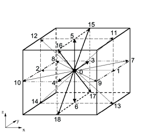
Figure 1: Schematic illustration of the three-dimensional, nineteen velocity (D3Q19) model.

$$\overrightarrow{e_{\alpha}}=\left\{\begin{array}[]{ll}{(0,0,0)}&{\alpha=0}\\ {(\pm 1,0,0),(0,\pm 1,0),(0,0,\pm 1)}&{\alpha=1,\cdots,6}\\ {(\pm 1,\pm 1,0),(\pm 1,0,\pm 1),(0,\pm 1,\pm 1)}&{\alpha=7,\cdots,18.}\end{array}\right.$$ (2)

The magnitude of the Cartesian component $c$ of the particle velocity $\overrightarrow{e_{\alpha}}$ is given by $c=\delta_{x}/\delta_{t}$, where $\delta_{t}$ is the lattice time step.

The first term on the right hand side (RHS) of Eq. (1) represents the cumulative effect of particle collisions on the evolution of distribution function $f_{\alpha}$. Collision is a relaxation process in which $f_{\beta}$ relaxes to its local equilibrium value $f_{\beta}^{eq}$ at a rate determined by the relaxation time matrix $\Lambda_{\alpha\beta}$. The GLBE has a generalized collision matrix with multiple relaxation times corresponding to the underlying physics: the macroscopic fields such as density, momentum and stress tensors are given as various kinetic moments of the distribution function. For example, collision does not alter the densities $\rho$ and momentum $\overrightarrow{j}=\rho\overrightarrow{u}$, while the stress tensors relax during collisins at rates determined by fluid properties such as viscosities. The components of the collision matrix $\Lambda_{\alpha\beta}$ in the GLBE are developed to reflect the underlying physics of collision as a relaxation process.

The second term on the RHS of Eq.( 1) introduces changes in the evolution of distribution function due to external force fields $\overrightarrow{F}$, such as driving body forces mimicking a pressure gradient in a periodic domain or gravity, or Lorentz or Coriolis forces, through a source term $S_{\alpha}$. In this term $I_{\alpha\beta}$ is the component of the identity matrix $I$. The source term $S_{\alpha}$ may be written as He et al. (1998); Premnath and Abraham (2007)

$$S_{\alpha}=\frac{(e_{\alpha j}-u_{j})F_{j}}{\rho c_{s}^{2}}f_{\alpha}^{eq,M}(\rho,\overrightarrow{u}),$$ (3)

where $f_{\alpha}^{eq,M}(\rho,\overrightarrow{u})$ is the local Maxwellian

$$f_{\alpha}^{eq,M}(\rho,\overrightarrow{u})=\omega_{\alpha}\rho\left\{1+\frac{\overrightarrow{e_{\alpha}}\cdotp\overrightarrow{u}}{c_{s}^{2}}+\frac{\left(\overrightarrow{e_{\alpha}}\cdotp\overrightarrow{u}\right)^{2}}{2c_{s}^{4}}-\frac{1}{2}\frac{\overrightarrow{u}\cdotp\overrightarrow{u}}{c_{s}^{2}}\right\},\omega_{\alpha}=\left\{\begin{array}[]{ll}{\frac{1}{3}}&{\alpha=0}\\ {\frac{1}{18}}&{\alpha=1,\cdots,6}\\ {\frac{1}{36}}&{\alpha=7,\cdots,18.}\end{array}\right.$$ (4)

and $c_{s}=c/\sqrt{3}$ is the speed of sound of the model. By neglecting terms of the order of $O(\mathrm{Ma}^{2})$ or higher Eq.(3) may be simplified as

$$S_{\alpha}=w_{\alpha}\left[\frac{3}{c^{2}}\left(e_{\alpha i}-u_{i}\right)+\frac{9}{c^{4}}\left(\overrightarrow{e_{\alpha}}\cdot\overrightarrow{u}\right)e_{\alpha i}\right]F_{i}$$ (5)

where $F_{i}=\{F_{x},F_{y},F_{z}\}$, with $F_{x}$, $F_{y}$ and $F_{z}$ are the Cartesian components of the external force field, which can, in general, vary in space and/or time.

It may be noted that, Eq. (1) is obtained from the second-order trapezoidal discretization of the source term in GLBE Premnath and Abraham (2007), viz., $f_{\alpha}(\overrightarrow{x}+\overrightarrow{e_{\alpha}}\delta_{t},t+\delta_{t})-f_{\alpha}(\overrightarrow{x},t)=-\sum_{\beta}\Lambda_{\alpha\beta}\left[f_{\beta}(\overrightarrow{x},t)-f_{\beta}^{eq}(\overrightarrow{x},t)\right]+1/2[S_{\alpha}(\overrightarrow{x},t)+S_{\alpha}(\overrightarrow{x}+\overrightarrow{e_{\alpha}}\delta_{t},t+\delta_{t})]\delta_{t}$, which is made effectively time-explicit through a transformation $\overline{f}_{\alpha}=f_{\alpha}-1/2S_{\alpha}\delta_{t}$ He et al. (1998), and then dropping the ‘overbar’ in subsequent representations for convenience. The second-order discretization provides a more accurate treatment of source terms, particulary in correctly recovering general forms of external non-uniform forces in the continuum limit without spurious terms due to discrete lattice effects Guo et al. (2002), and its time-explicit representation facilitates numerical solution in a manner analogous to the standard LBE. The local macroscopic density and velocity fields are given by

$$\rho=\sum_{\alpha}f_{\alpha},$$ (6)

$$\overrightarrow{j}\equiv\rho\overrightarrow{u}=\sum_{\alpha}f_{\alpha}\overrightarrow{e_{\alpha}}+\frac{1}{2}\overrightarrow{F}\delta_{t},$$ (7)

and the pressure field $p$ may be written as

$$p=c_{s}^{2}\rho.$$ (8)

The physics behind the kinetic equation Eq. (1), and in particular, the collision matrix $\Lambda_{\alpha\beta}$ will become more transparent when it is specified directly in terms of a set of linearly independent moments $\mathbf{\widehat{f}}$ instead of the distribution functions $\mathbf{f}=\left[f_{0},f_{1},f_{2},\ldots,f_{18}\right]^{{\dagger}}$, i.e. through $\mathbf{\widehat{f}}=\left[\widehat{f}_{0},\widehat{f}_{1},\widehat{f}_{2},\ldots,\widehat{f}_{18}\right]^{{\dagger}}$. Here, the superscript ‘${\dagger}$’ is the transpose operator and the ‘hat’ represents quantities in moment space. The moments have direct physical import to the macroscopic quantities such as momentum and viscous stress tensor. The components of $\mathbf{\widehat{f}}$ are provided in Appendix A. This is achieved through a transformation matrix $\mathcal{T}$: $\mathbf{\widehat{f}}=\mathcal{T}\mathbf{f}$. The elements of $\mathcal{T}$ are given in d’Humières et al. d‘Humières et al. (2002). Each row of this matrix is orthogonal to every other row. The essential principle for its construction is based on the observation that the collision matrix $\Lambda$ becomes a diagonal matrix $\widehat{\Lambda}$ through $\widehat{\Lambda}=\mathcal{T}\Lambda\mathcal{T}^{-1}$ in a suitable orthogonal basis which can be obtained as combinations of monomials of the Cartesian components of the particle velocity directions $\overrightarrow{e_{\alpha}}$ through the standard Gram-Schmidt procedure.

The collision matrix in moment space $\widehat{\Lambda}$ may thus be written as

$$\widehat{\Lambda}=diag\left(s_{0},s_{1},s_{2},\ldots,s_{18}\right),$$ (9)

where $s_{0},s_{1},s_{2},\ldots,s_{18}$ relaxation time rates for the respective moments. The corresponding components of the local equilibrium distributions in moment space $\mathbf{\widehat{f}}^{eq}=\left[\widehat{f}_{0}^{eq},\widehat{f}_{1}^{eq},\widehat{f}_{2}^{eq},\ldots,\widehat{f}_{18}^{eq}\right]^{{\dagger}}$ are functions of the conserved moments, viz., local density and momentum fields, and are given in Appendix A .

When there is an external force field, as in Eq. (5) represented in particle velocity space $\mathbf{S}$, where $\mathbf{S}=\left[S_{0},S_{1},S_{2},\ldots,S_{18}\right]^{{\dagger}}$, appropriate source terms in moment space $\mathbf{\widehat{S}}$ need to be introduced. In this regard, we obtain the projections of source terms onto moments $\mathbf{\widehat{S}}$ by a direct application of the transformation matrix to Eq. (5) for the D3Q19 model, as done for the D3Q15 model earlier in Ref.  Premnath and Abraham (2007), i.e. $\mathbf{\widehat{S}}=\mathcal{T}\mathbf{S}$, where $\mathbf{\widehat{S}}=\left[\widehat{S}_{0},\widehat{S}_{1},\widehat{S}_{2},\ldots,\widehat{S}_{18}\right]^{{\dagger}}$. They are explicit functions of the external force field $\overrightarrow{F}$ and the velocity $\overrightarrow{u}$, which are summarized in Appendix A. In effect, due to collisions and the presence of external forces, the distribution functions in moment space or simply, the moments are modified by the quantity $-\Lambda\left(\mathbf{\widehat{f}}-\mathbf{\widehat{f}}^{eq}\right)+\left(\mathrm{I}-1/2\widehat{\Lambda}\right)\mathbf{\widehat{S}}\delta_{t}$.

A multiscale analysis based on the Chapman–Enskog expansion Chapman and Cowling (1964) of the GLBE shows that in the continuum limit, it corresponds to the weakly compressible Navier–Stokes equations with external forces, where the density, velocity and pressure, given by Eqs. (6), (7) and  (8), respectively, as was done for the D3Q15 model by Premnath and Abraham Premnath and Abraham (2007). The macrodynamical equations can also be derived through an asymptotic analysis under a diffusive scaling Sone (1990); Junk (2001); Junk et al. (2005). The transport properties of the fluid flow, such as bulk $\zeta$ and shear $\nu$ kinematic viscosities can be related to the appropriate relaxation times through either Chapman–Enskog analysis of the GLBE or the von Neumann stability analysis of its linearized version Lallemand and Luo (2000):

$$\zeta = \frac{2}{9}\left(\frac{1}{s_{1}}-\frac{1}{2}\right)\delta_{t},$$ (10)

$$\nu = \frac{1}{3}\left(\frac{1}{s_{\beta}}-\frac{1}{2}\right)\delta_{t},\quad\beta=9,11,13,14,15.$$ (11)

Notice that from Eq. (11), $s_{9}=s_{11}=s_{13}=s_{14}=s_{15}$ to maintain isotropy of the stress tensor and $s_{2}$ determines the magnitude of bulk viscosity. The rest of the relaxation parameters do not affect hydrodynamics but can be chosen in such a way to enhance numerical stability as to simulate higher Reynolds number problems for a given grid resolution, in particular for wall-bounded turbulent flows considered here. Based on linear stability analysis Lallemand and Luo (2000), the following values for the other relaxation parameters are determined d‘Humières et al. (2002): $s_{1}=1.19$, $s_{2}=s_{10}=s_{12}=1.4$, $s_{4}=s_{6}=s_{8}=1.2$ and $s_{16}=s_{17}=s_{18}=1.98$. For the conserved moments, the values of the relaxation parameters are immaterial as their corresponding equilibrium distribution is set to the value of the respective moments itself. However, with forcing terms it is important that they be non-zero McCracken and Abraham (2005a); Premnath and Abraham (2007). For simplicity, we set $s_{0}=s_{3}=s_{5}=s_{7}=1.0$. It may be noted that all relaxation parameters have the following bound $0<s_{\alpha}<2$. In this paper, we employ the above values for the relaxation parameters. Since the GLBE employs a set of relaxation times, it is also referred to as the multiple-relaxation time (MRT)-LBE.

It may be noted that when all the relaxation times are equal, i.e., $s_{1}=s_{2}=\ldots=s_{18}=1/\tau$, where $\tau$ is the relaxation time, the GLBE reduces to the single-relaxation time (SRT)-LBE Qian et al. (1992); Chen et al. (1992) based on the Bhatnagar, Gross and Krook model Bhatnagar et al. (1954). Its popularity and appeal lies in its apparent simplicity. However, the GLBE has marked advantages when compared with the SRT-LBE: for a given resolution, the GLBE is significantly more stable numerically and more accurate for problems with anisotropy, with an insignificant additional computational overhead, thereby allowing access to a greater range of problems, particularly at higher Reynolds numbers, to be reached than possible with the SRT-LBE. This is demonstrated later for two problems involving wall-generated turbulent flows.

III Subgrid Scale Turbulence Model

In this paper, we have incorporated the subgrid scale (SGS) effects in the GLBE through the standard Smagorinsky model Smagorinsky (1963). It assumes that the SGS Reynolds stress term depends on the local strain rate tensor and leads to the eddy-viscosity assumption. The eddy viscosity $\nu_{t}$ arising from this model can be written as

$$\nu_{t}=\left(C_{s}\Delta\right)^{2}\overline{S},\quad\overline{S}=\sqrt{2S_{ij}S_{ij}},$$ (12)

where $C_{s}$ is a constant (taken equal to 0.12 in this paper). Here, $\Delta$ is the cut-off length scale set equal to the lattice-grid spacing, i.e. $\Delta=\delta_{x}$, and $S_{ij}$ is the strain rate tensor given by $S_{ij}=1/2\left(\partial_{j}u_{i}+\partial_{i}u_{j}\right)$. In LBM, the strain rate tensor can be computed directly from the non-equilibrium part of the moments, without the need to apply finite differencing to the velocity field. Recently, Yu et al. Yu et al. (2006) derived such expressions for the strain-rate tensor for the D3Q19 model of the GLBE without forcing term. In this paper, we extend the results for GLBE with forcing term by means of a Chapman–Enskog analysis Chapman and Cowling (1964); Premnath and Abraham (2007), which is presented in Appendix B. The use of forcing terms allows for incorporation of not only general forms of non-uniform external forces, but also more general forms of SGS Reynolds stress models Premnath et al. (2008). This procedure for calculation of strain rates in GLBE is fully local in space and is computationally efficient, particularly for complex geometries.

The eddy viscosity $\nu_{t}$ is added to the molecular viscosity $\nu_{0}$, obtained from the statement of the problem, through the characteristic dimensionless number, such as shear Reynolds number for turbulent channel flow problem, to yield the total viscosity $\nu$ (i.e., $\nu=\nu_{0}+\nu_{t}$). The relaxation times may then be obtained from Eq. (11). When such eddy-viscosity type SGS models are used to provide additional contributions to the relaxation times, the GLBE can be considered to be “coarse-grained” and it can be readily shown that the macroscopic dynamical equations of fluid flow corresponds to the filtered equations with the SGS Reynolds stress represented through the eddy viscosity. As a result, the GLBE would represent the dynamics of larger eddies in turbulent flows. The distribution functions (or equivalently, the moments) and the hydrodynamic fields, can be considered to be grid-filtered quantities. An alternative approach is to directly apply filters to the moment representation of the GLBE and rigorously derive SGS models essentially from kinetic theory under appropriate scaling Ansumali et al. (2004).

To account for the damping of scales near the walls, following an earlier work Moin and Kim (1982), we have implemented the van Driest damping function van Driest (1956)

$$\Delta=\delta_{x}\left[1-\exp\left(-\frac{z^{+}}{A^{+}}\right)\right]$$ (13)

where $z^{+}$ is the distance from the wall and $A^{+}$ is a constant, taken to be $25$ in this work Moin and Kim (1982). The superscript $+$ signifies normalization with respect to wall units, i.e. $z^{+}=z/\delta_{\nu}$, where $\delta_{\nu}=u_{*}/\nu_{0}$ is the characteristic viscous length scale. Here, $u_{*}$ is the shear or friction velocity, which is related to the wall shear stress $\tau_{w}$ through $u_{*}=\sqrt{\tau_{w}/\rho}$. While this approach has some empiricism built-in, for a class of wall-bounded turbulent flows, such as turbulent channel flows considered here, it has been shown to be reasonably accurate in prior work based on the solution of grid-filtered Navier–Stokes equations Moin and Kim (1982). Also, as will be shown later in this paper that the GLBE is able to reproduce turbulence statistics in the near-wall region reasonable well using this damping supplemented to the SGS model. For more general situations, for improved accuracy it may be necessary to introduce dynamic SGS models (e.g.,  Germano et al. (1991); Zang et al. (1993); Salvetti and Banerjee (1995)) for LES using the GLBE Premnath et al. (2008).

IV Computational Procedure: Optimization with Forcing Terms

In practice, implementation of the GLBE with forcing term, i.e. Eq. (1), together with associated turbulence models and procedure for strain rate computations, initial and boundary conditions, requires careful consideration for the details for efficient performance. In particular, the “effective” collision step including the forcing terms should be performed in moment space, while the streaming step should be executed in particle velocity space and the special properties of the transformation matrix that transform between the two spaces should be fully exploited d‘Humières et al. (2002); Yu et al. (2006); Premnath and Abraham (2007). Such properties of the transformation matrix $\mathcal{T}$ include its orthogonality, entries with many zero elements, and entries with many common elements that are integers, which are used to form the most compact common sub-expressions for transformations between spaces. We will now briefly discuss the details of the computational procedure for the GLBE with forcing term used in this paper.

The GLBE with forcing term can be re-written in terms of the following “effective” collision and streaming steps, respectively:

$$\mathbf{\widetilde{f}}(\overrightarrow{x},t)=\mathbf{f}(\overrightarrow{x},t)+\bm{\varpi}(\overrightarrow{x},t),$$ (14)

and

$$f_{\alpha}(\overrightarrow{x}+\overrightarrow{e}_{\alpha}\delta_{t},t+\delta_{t})=f_{\alpha}(\overrightarrow{x},t),$$ (15)

where $\widetilde{f}_{\alpha}$ is the post-collision distribution function and

$$\bm{\varpi}(\overrightarrow{x},t)=\mathcal{T}^{-1}\left[-\widehat{\Lambda}\left(\mathbf{\widehat{f}}-\mathbf{\widehat{f}}^{eq}\right)+\left(\mathcal{I}-\frac{1}{2}\widehat{\Lambda}\right)\mathbf{\widehat{S}}\right],$$ (16)

is the effective change due to collision including the effect of external forces. Here, $\mathbf{\widehat{f}}\equiv\mathbf{\widehat{f}}(\overrightarrow{x},t)$, $\mathbf{\widehat{f}}^{eq}\equiv\mathbf{\widehat{f}}^{eq}(\overrightarrow{x},t)$ and $\mathbf{\widehat{S}}\equiv\mathbf{\widehat{S}}(\overrightarrow{x},t)$, and $\mathcal{I}$ is the identity matrix and $\widehat{\Lambda}=\mathcal{T}\Lambda\mathcal{T}^{-1}=diag(s_{0},s_{1},\ldots,s_{18})$ is the diagonal collision matrix in moment space.

A note regarding the actual implementation details is in order. First, the transformation matrix $\mathcal{T}$ is row-wise orthogonal and satisfies $\mathcal{T}\mathcal{T}^{{\dagger}}=\mathcal{\widehat{L}}$, where $\mathcal{T}^{{\dagger}}$ is the transpose of $\mathcal{T}$ and $\mathcal{\widehat{L}}$ is a diagonal normalization matrix. Thus it follows that the matrix inverse $\mathcal{T}^{-1}$ is obtained simply using $\mathcal{T}^{-1}=\mathcal{T}^{{\dagger}}\mathcal{\widehat{L}}$. As a result, we may write Eq. (16) as $\bm{\varpi}(\overrightarrow{x},t)=\mathcal{T}^{{\dagger}}\mathbf{\widehat{q}}$ where $\mathbf{\widehat{q}}$ is given by $\mathbf{\widehat{q}}=\left[-\widehat{\Gamma}\left(\mathbf{\widehat{f}}-\mathbf{\widehat{f}}^{eq}\right)+\left(\mathcal{\widehat{L}}^{-1}-\frac{1}{2}\widehat{\Gamma}\right)\mathbf{\widehat{S}}\right]$ and $\widehat{\Gamma}=\mathcal{\widehat{L}}^{-1}\widehat{\Lambda}$. Thus, for computational efficiency, we actually implement the “effective” collision step that also including forcing terms in moment space. Now, the relaxation times in $\widehat{\Lambda}$ used to compute in Eq. (16) can be related to the transport coefficients and modulated by eddy viscosity, in the case of hydrodynamic time scales, as follows: $s_{1}^{-1}=s_{\zeta}^{-1}=\frac{9}{2}\zeta+\frac{1}{2}$ from Eq. (10), and $s_{9}=s_{11}=s_{13}=s_{14}=s_{15}=s_{\nu}$, where $s_{\nu}^{-1}=3\nu+\frac{1}{2}=3(\nu_{0}+\nu_{t})+\frac{1}{2}$, from Eq. (11). The eddy viscosity $\nu_{t}$ is obtained from Eq. (12). The rest of the relaxation parameters can be chosen to enhance numerical stability, as discussed in Section II. The forcing term used in the computation of strain rate tensor (Appendix B) and in the “effective” collision step (Eq. (16)) can be obtained from Appendix A. This optimized procedure dramatically improves the computational speed of the GLBE as compared to a naive implementation. Indeed, the additional computational overhead of using GLBE in lieu of the SRT-LBE is small, between $15\%-30\%$, but, as will be shown later, with a significantly improved accuracy and numerical stability.

No slip wall boundary conditions, involving stationary walls as well as moving walls, in the case of turbulent channel flow and driven cavity flow, respectively, are implemented by means of the link or half-way bounce back Ladd (1994). To initiate turbulence, a three-dimensional perturbation velocity field satisfying divergence free condition Lam (1989) is employed in the solution of the GLBE through the consistent initialization procedure Mei et al. (2006).

V Fully-Developed Turbulent Channel Flow

First, we simulated a canonical problem, viz., fully-developed turbulent channel flow using the GLBE with the SGS model mentioned above. Prior efforts have validated LBM as a DNS tool for this problem by comparing a set of turbulent statistics with available data Amati et al. (1997, 1999); Lammers et al. (2006). The focus of this study is to evaluate MRT-LBE that incorporate subgrid scale effects for this problem on a relatively coarse grid, while maintaining the necessary near-wall resolution.

We considered turbulent flow with a shear Reynolds number $\mathrm{Re}_{*}=u_{*}H/\nu_{0}=183.6$, where $\nu_{0}$ is the molecular kinematic viscosity and $H$ is the channel half height. A schematic of the problem set up is shown in Fig. 2, in which a no-slip boundary is imposed at the bottom, free-slip at the top and periodic boundary conditions were applied in the streamwise $x$ and spanwise $y$ directions Lam (1989); Lam and Banerjee (1992).

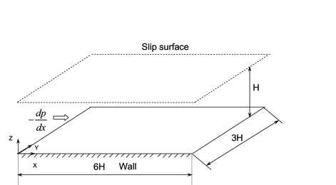
Figure 2: Schematic of computational domain for LES of fully-developed turbulent channel flow.

The computational domain is chosen with appropriate aspect ratios, viz., $6H$ and $3H$ in the streamwise and spanwise directions, respectively. With this domain, a sufficient number of wall-layer streaks are accommodated Lam (1989) and end effects of two-point correlations are excluded, i.e. the two-point velocity correlations in solutions are required to decay nearly to zero within half the domain Moin and Mahesh (1998). For this initial case, we considered a uniform grid with a grid spacing in wall units (referred to with a “$+$” superscript) as $\Delta^{+}=\Delta/\delta_{\nu}=4.08$, where $\delta_{\nu}=\nu_{0}/u_{*}$ is the viscous length scale as defined in Sec. III. The computational domain thus consists of $270\times 135\times 47$ grid nodes. Due to the use of link-bounce back method for implementation of wall boundary condition, the first lattice node is located at a distance of $\Delta^{+}_{nw}=\Delta^{+}/2$, which in our case is 2.04. For wall-bounded turbulent flows, it is important to adequately resolve the near-wall, small-scale turbulent structures, which is satisfied when the computations resolve the local dissipative or Kolmogorov length scale $\eta=(\nu^{3}_{0}/\epsilon)^{1/4}$, i.e. $\Delta^{+}_{nw}\leq O(\eta^{+})$ Moin and Mahesh (1998). In particular, it is generally recognized that $1.5\eta^{+}-2.0\eta^{+}$ represents the upper limit of grid-spacing, above which the small scale turbulent motions in bounded flows are not well resolved. It can be shown by simple arguments that $\eta^{+}\approx 1.5-2.0$ at the wall and that $\eta^{+}$ increases with increasing distance from the wall Pope (2000). Thus, our computational set up is expected to fairly resolve the small-scale turbulent structures.

The initial mean velocity is specified to satisfy the $1/7^{th}$ power law Pope (2000), while initial perturbations satisfying divergence free velocity field Lam (1989). The density field is taken to be $\rho=\rho_{0}=1.0$ for the entire domain. The precise form of the initial fields may not affect affect the turbulence statistics, but can have significant influence on the number of time steps needed for convergence of the solution to statistically steady state. In particular, the above choice of initial fields would enable a rapid convergence to the statistically steady state solution of the fluctuating fields obtained by the GLBE with forcing term. With these initial conditions on the macroscopic fields, we employed the consistent initialization procedure for the distribution functions or moments Mei et al. (2006). Using $\overrightarrow{F}=-\frac{dp}{dx}\widehat{x}=\frac{\tau_{w}}{H}\widehat{x}=\frac{\rho u_{*}^{2}}{H}\widehat{x}$ as the driving force, the GLBE computations are carried out until stationary turbulence statistics are obtained, as measured by the invariant Reynolds stresses profiles. This initial run was carried out for a duration of $50T^{*}$, where $T^{*}=H/u_{*}$ is the characteristic time scale. The averaging of various flow quantities was carried out in time as well as in space in the homogeneous directions, i.e. over the horizontal planes, by an additional run for a period of $30T^{*}$.

Figure 3 shows the computed mean velocity profile, normalized by the shear velocity $u_{*}$, as a function of the distance from the wall given in wall units, i.e. $z^{+}=z/\delta_{\nu}$, where $\delta_{\nu}$ is the viscous length scale defined earlier.

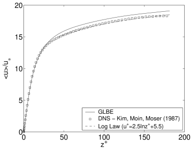
Figure 3: Comparison of the computed mean velocity profile with wall-layer scaling laws in outer wall coordinates for fully-developed turbulent channel flow at $\mathrm{Re}_{*}=183.6$.

Also plotted are the DNS data by Kim, Moin and Moser (1987) Kim et al. (1987) based on a spectral method and the von Karman log-law of the wall, which is valid for the so-called log-region. The computed velocity profile follows the DNS data fairly closely, with about $5\%$ difference. Such differences are characteristic of LES, which employ relatively coarser grids than DNS, and they also generally depend on the numerical dissipation of the computational approach for LES (see e.g., Ref. Choi et al. (2000); Gullbrand and Chow (2003)).

Figure 4 shows comparison of the computed mean velocity profile as a function of the distance from the wall with wall-layer scaling laws, i.e. viscous sublayer and log-law of the wall.

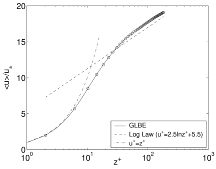
Figure 4: Comparison of the computed mean velocity profile with wall-layer scaling laws in inner wall coordinates for fully-developed turbulent channel flow at $\mathrm{Re}_{*}=183.6$.

Generally, Reynolds stress effects are negligible in the viscous sublayer region ($z^{+}\leq 5$), and $u^{+}\equiv<u>/u_{*}=z^{+}$ holds for the mean velocity. For $z^{+}>30$, the mean velocity satisfies the log-law, i.e. $u^{+}=A\mathrm{ln}z^{+}+B$, where the coefficients depend on the flow parameters and nature of the wall. Values of $A=2.5$ and $B=5.5$ are known to be reasonably accurate for flow over smooth walls at $\mathrm{Re}_{*}\approx 180$ Lam (1989); Kim et al. (1987); Pope (2000). It can be seen that computations agree well with these scaling laws.

The Reynolds stress, normalized by the wall-shear stress, is presented in Fig. 5 in semi-log scale and compared with the DNS data of Kim, Moin and Moser Kim et al. (1987) obtained from the direct solution of incompressible Navier–Stokes equations (NSE), which the GLBE computations reproduce quite well with good accuracy.

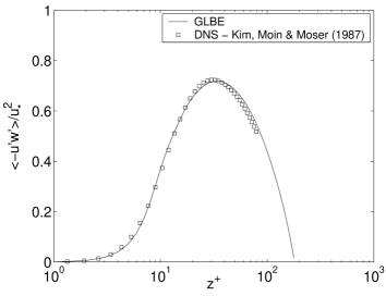
Figure 5: Reynolds stress normalized by the wall shear stress for fully-developed turbulent channel flow at $\mathrm{Re}_{*}=183.6$.

Let us now consider the statistics of turbulent fluctuations of important quantities in the near-wall region. Figures 6, 7 and 8 show comparisons of the components of the root-mean-square (rms) streamwise, spanwise and wall-normal velocity fluctuations, respectively, computed using the GLBE with data from DNS based on the solution of NSE by Kim, Moin and Moser Kim et al. (1987) and experimental measurements of Kreplin and Eckelmann Kreplin and Eckelmann (1979). It may be seen that the computed results agree reasonably well with prior data.

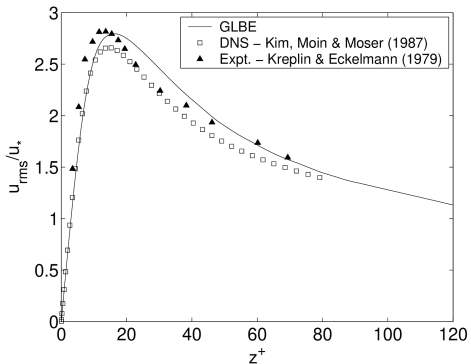
Figure 6: Root-mean-square (rms) streamwise velocity fluctuations normalized by the wall shear velocity for fully-developed turbulent channel flow at $\mathrm{Re}_{*}=183.6$.

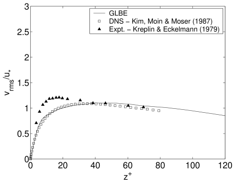
Figure 7: Root-mean-square (rms) spanwise velocity fluctuations normalized by the wall shear velocity for fully-developed turbulent channel flow at $\mathrm{Re}_{*}=183.6$.

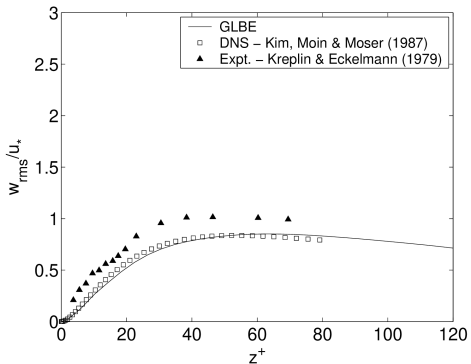
Figure 8: Root-mean-square (rms) wall-normal velocity fluctuations normalized by the wall shear velocity for fully-developed turbulent channel flow at $\mathrm{Re}_{*}=183.6$.

Another important quantity representing turbulent activity near the wall is the pressure fluctuations. Figure 9 shows the computed rms pressure fluctuations. The profile shown here is qualitatively consistent with the NSE-DNS results.

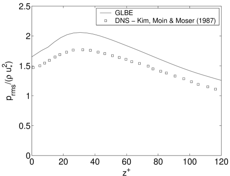
Figure 9: Root-mean-square (rms) pressure fluctuations normalized by the wall shear stress for fully-developed turbulent channel flow at $\mathrm{Re}_{*}=183.6$.

It is found that the pressure fluctuations normalized by the wall shear stress is about 1.66 at the wall, which is within the range in prior data – NSE based DNS results in Ref. Kim et al. (1987) and Lam (1989) provide values of about 1.5 and 2.15 respectively. These values depend on the Reynolds number employed. In the measurements reported by Willmarth Willmarth (1975), the values of maximum rms pressure fluctuations were found to be between 2 and 3, but these were for much higher Reynolds numbers than considered here. Moreover, the computed maximum pressure fluctuations occurs at $z^{+}\approx 26$, which is close to the range in DNS data Kim et al. (1987), i.e. $z^{+}\approx 30$. It may be seen that there the computed profile rms pressure fluctuations using GLBE is systematically somewhat larger than the DNS results based on NSE. This observation is also consistent with those found in Ref. Lammers et al. (2006), where DNS using SRT-LBE revealed similar values for the peak rms pressure fluctuations and its location. Such difference could plausibly be due to compressibility effects inherent in LBM, while the DNS carried out in Ref. Kim et al. (1987) considered incompressible NSE.

A particularly stringent test is the comparison of computed components of near wall rms vorticity fluctuations with DNS, which is shown in Fig. 10, in which lines represent the GLBE solution and symbols the DNS data Kim et al. (1987). The components of vorticity fluctuations normalized by the mean wall shear ($u_{*}^{2}/\nu_{0}$).

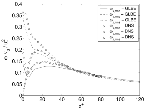
Figure 10: Components of root-mean-square (rms) vorticity fluctuations normalized by a factor given in terms of wall shear stress for fully-developed turbulent channel flow at $\mathrm{Re}_{*}=183.6$. Lines are GLBE solution and symbols are DNS data Kim et al. (1987).

There is a strong variation among the components of vorticity due to inhomogeneity and anisotropy of turbulence closer to the wall. Also, as expected, for distances further from the wall, all the components of vorticity are essentially the same. While there are some deviations from the DNS results, the GLBE is able to reproduce the qualitative trends and, more importantly, the ratio between components of vorticity. Such deviations have been observed in LES using filtered NSE, e.g. Dubief and Delcayre (2000), who point out the underestimation of the resolved components to be due to mere consequence of filtering process inherent to LES.

Another important measure is the pressure-strain (PS) correlations. Their components are: $PS_{x}=\langle p^{{}^{\prime}}\partial_{x}u_{x}^{{}^{\prime}}\rangle$, $PS_{y}=\langle p^{{}^{\prime}}\partial_{y}u_{y}^{{}^{\prime}}\rangle$, and $PS_{z}=\langle p^{{}^{\prime}}\partial_{z}u_{z}^{{}^{\prime}}\rangle$, where the prime denotes fluctuations and the brackets refer to averaging (along homogeneous spatial directions and time). They provide indications of energy transfers among the components. Figure 11 shows the components of the computed PS correlations.

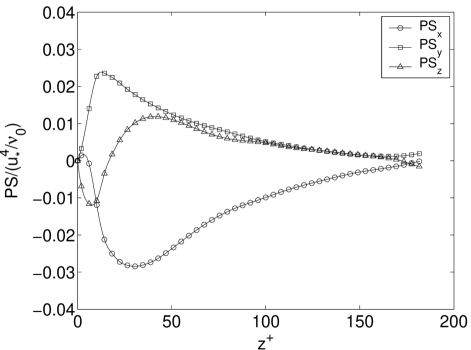
Figure 11: Components of computed pressure-strain correlations normalized by a factor given in terms of wall shear velocity and molecular viscosity for fully-developed turbulent channel flow at $\mathrm{Re}_{*}=183.6$.

They exhibit the expected behavior close to the wall, including the transfer of energy from the wall-normal component to the other two components near the wall – a phenomenon termed as splatting or impingement Moin and Kim (1982). Thus, it appears that the GLBE with forcing term is a reliable approach for computation of fully-developed turbulent channel flows.

V.1 Numerical Stability

To put things in perspective, let us now discuss the stability characteristics of the GLBE in relation to the SRT-LBE for turbulent channel flow on coarser grids. The test case used a shear Reynolds number $\mathrm{Re}_{*}$ of $180$, with a uniform spacing $\Delta^{+}$ of $6$ in wall units, which at the near-wall node becomes $\Delta^{+}_{nw}=3$ due to the link-bounce back scheme employed. The number of grid nodes used in each case is $180\times 90\times 32$. This is a somewhat coarser resolution than used in the previous simulation and it is expected that small-scale near-wall dynamics may not be properly resolved. Nevertheless, subgrid scale motions are quite energetic for such coarse resolutions and it is important to determine if the grid scale numerical instabilities developed by the computational approaches interact with them. The numerical stability of the LBM depends on various factors including the grid resolution $\Delta$, maximum velocity or Mach number $\mathrm{Ma}$ considered and the relaxation times or the molecular viscosity of the fluid $\nu_{0}$. For a given resolution and maximum flow velocity, the numerical stability of the LBE depends mainly on the molecular viscosity of the fluid $\nu_{0}$.

As is natural for LBE, unless otherwise specified, all the results are reported in lattice units. That is, the velocities are scaled by the particle velocity $c$ and the distance by the streaming distance of the populations, $\delta_{x}$. Here, we considered a maximum velocity, i.e. velocity at the top surface to be about $0.18$, and varied the viscosity $\nu_{0}$. In the case of the SRT-LBE, the only parameter that can be used to specify $\nu_{0}$ is the single-relaxation time $\tau$ and its value is chosen from $\nu_{0}=1/3(\tau-1/2)$. On the other hand, for the GLBE, the relaxation parameters that determine moments involving fluid stresses are determined from Eq. 11, while the rest of the parameters are tuned to improve numerical stability as specified earlier.

Figure 12 shows the components of rms turbulent fluctuations obtained by using both the GLBE and the SRT-LBE at $\nu_{0}=0.0012$.

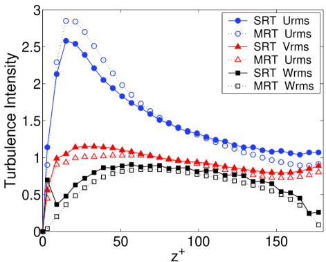
Figure 12: Comparison of the components of root-mean-square (rms) velocity fluctuations normalized by the wall shear velocity for fully-developed turbulent channel flow with a free-slip surface at the top for $\mathrm{Re}_{*}=180$ obtained by GLBE or MRT-LBE (dashed lines with open symbols) and BGK-LBE or SRT-LBE (solid line with filled symbols) on a coarse grid.

The rms turbulent fluctuations results from the SRT-LBE simulation show some physically unrealistic behavior, with a large spike in the wall normal component near the no-slip wall. Farther out, ripples which grow as the slip-surface is approached can be seen in both the wall normal and the streamwise component. That is, spurious oscillations due to non-hydrodynamic or kinetic modes seem to strongly interact with fluctuating turbulent motions generated by the wall, particularly in the wall-normal component, in the case of the SRT-LBE. In contrast, due to scale separation of relaxation parameters in the GLBE, the kinetic modes are quickly damped and do not exhibit such unphysical behavior.

It may be noted that such spurious effects do not seem to manifest with the SRT-LBE, when fine enough resolution is employed, as was also noticed, for e.g. in Ref. Lammers et al. (2006). On the other hand, for the same resolution, if the viscosity is lowered further, the SRT-LBE becomes unstable. Stable and physically realistic solutions can be obtained only for viscosity greater than 0.0018 in this particular case. On the other hand, the GLBE seems to predict correct physical and smoother behavior for all the components of velocity fluctuations for viscosity of 0.0012 shown in Fig. 12 and up to 0.0006 in our work. For this specific problem we thus obtain enhancement in stability by a factor of about $3$, which is consistent with the observations made for other problems d‘Humières et al. (2002); Dellar (2003); McCracken and Abraham (2005a); Premnath and Abraham (2005, 2007); Yu et al. (2006). Thus, it appears that the GLBE is superior in terms of both physical fidelity and stability on coarser grid LES simulations of anisotropic and inhomogeneous turbulent flows, when it is used in lieu of the SRT-LBE. We will also discuss more on the stability aspects when we discuss about the other canonical problem considered in this paper.

V.2 Conservative Multiblock Approach for Local Grid Refinement

Close to a wall, length scales are very small, requiring a fine grid to adequately resolve turbulent structures. Use of a grid fine enough to resolve the wall regions throughout the domain can entail significant computational cost, and this can be mitigated by introducing coarser grids farther from the wall, where turbulent length scales are larger. One approach is to consider using continuously varying grid resolutions, using a interpolated-supplemented LBM He et al. (1996) that effectively decouples particle velocity space represented by the lattice and the computational grid. However, it is well known that interpolation could introduce significant numerical dissipation, see for e.g. Lallemand and Luo (2000), which could severely affect the accuracy of solutions involving turbulent fluctuations, as was confirmed in numerical experiments during the course of this work. Thus, we consider locally embedded grid refinement approaches, and in particular their conservative versions Chen et al. (2006); Rohde et al. (2006) that enforce mass and momentum conservation. Similar zonal embedded approaches have been successfully employed in computational approaches based on the solution of filtered NSE for LES of turbulent flows Kravchenko et al. (1996).

Figure 13 shows a schematic of such a multiblock approach in which a fine cubic lattice grid is used close to the wall and a coarser one, again cubic in shape, farther out.

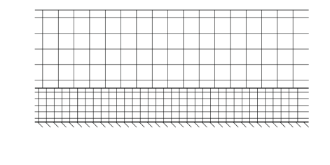
Figure 13: Schematic of conservative local refinement using multiblock grids with GLBE.

In order to facilitate the exchange of information at the interface between the grids, the spacing of the nodes changes by an integer factor, in this case two. As well as using different grid sizes, the two regions use different time steps (time step being proportional to grid size), and the computational cost required per unit volume is thus reduced by a factor of 16 in the coarse grid. Figure 13 shows a staggered grid arrangement, in which nodes on the fine and coarse sides of the interface are arranged in a manner that facilitates the imposition of mass and momentum conservation. Different blocks communicate with each other through the Coalesce and the Explode steps, in addition to the standard stream-and-collide procedure. The details are provided in Chen et al. Chen et al. (2006) and Rohde et al. Rohde et al. (2006), and here we very briefly present the essential elements in what follows. The Coalesce procedure involves summing the particle populations on the fine nodes to provide new incoming particle populations for the corresponding coarse nodes. Similarly, the Explode step involves redistributing the populations on the coarse node to the surrounding fine nodes. These grid-communicating steps used in the multiblock approach presented in Chen et al. Chen et al. (2006) were incorporated in the GLBE framework in this work.

We performed fully-developed turbulent channel flow at the same shear Reynolds number as before, i.e. $183.6$, with different blocks, viz., fine block near the wall and coarse block in the bulk bounded by top free-slip surface. For the fine grid, we used a resolution $\Delta^{+}_{fine}=4$ in wall-units (with $\Delta^{+}_{nw}=2$ due to link-bounce back) and a resolution of $\Delta^{+}_{coarse}=8$ in wall units for the coarse grid. We used $256\times 128\times 17$ grids for the fine block and $128\times 64\times 17$ for the coarse block, which corresponds to similar aspect ratios to that used in the earlier simulations. The initial run and averaging times used were similar to that for the uniform grid case, viz., $50T^{*}$ and $30T^{*}$, respectively.

The mean velocity and Reynolds stress profiles computed using the GLBE with locally refined multiblock grids are compared with uniform grid solution, again computed using GLBE, along with the DNS data Kim et al. (1987), in Figs. 14 and 15, respectively.

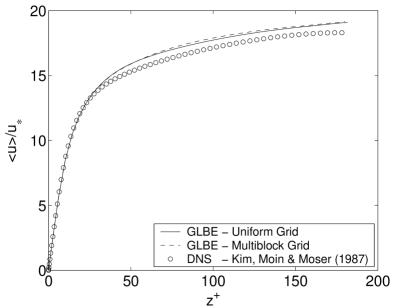
Figure 14: Mean velocity normalized by the wall shear velocity for fully-developed turbulent channel flow at $\mathrm{Re}_{*}=183.6$. Lines are GLBE results on locally refined multiblock (broken) and uniform (solid) grids, and symbols are Kim, Moin and Moser’s DNS data (1987) Kim et al. (1987).

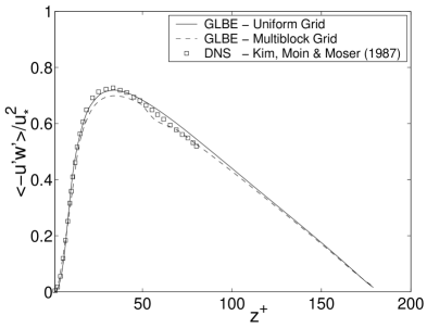
Figure 15: Reynolds stress normalized by the wall shear stress for fully-developed turbulent channel flow at $\mathrm{Re}_{*}=183.6$. Lines are GLBE results on locally refined multiblock (broken) and uniform (solid) grids, and symbols Kim, Moin and Moser’s DNS data (1987) Kim et al. (1987).

Generally, good agreement between various simulations can be seen. Some differences between the DNS data and the LES results based on the GLBE noticed in these figures are similar to those found in LES based on filtered NSE. The components of the rms velocity fluctuations in streamwise, spanwise and wall-normal directions are presented in Figs. 16, 17 and 18, respectively.

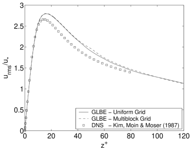
Figure 16: Root-mean-square (rms) streamwise velocity fluctuations normalized by the wall shear velocity for fully-developed turbulent channel flow at $\mathrm{Re}_{*}=183.6$. Lines are GLBE results on locally refined multiblock (broken) and uniform (solid) grids, and symbols are Kim, Moin and Moser’s DNS data (1987) Kim et al. (1987).

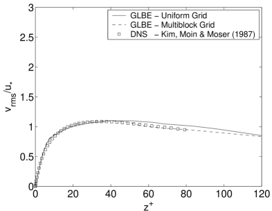
Figure 17: Root-mean-square (rms) spanwise velocity fluctuations normalized by the wall shear velocity for fully-developed turbulent channel flow at $\mathrm{Re}_{*}=183.6$. Lines are GLBE results on locally refined multiblock (broken) and uniform (solid) grids, and symbols are Kim, Moin and Moser’s DNS data (1987) Kim et al. (1987).

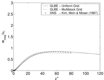
Figure 18: Root-mean-square (rms) wall normal velocity fluctuations normalized by the wall shear velocity for fully-developed turbulent channel flow at $\mathrm{Re}_{*}=183.6$. Lines are GLBE results on locally refined multiblock (broken) and uniform (solid) grids, and symbols are Kim, Moin and Moser’s DNS data (1987) Kim et al. (1987).

Again, the multiblock GLBE based LES results are fairly in good agreement with the uniform grid GLBE as well as the DNS data for various components of velocity fluctuations. It is found that the velocity fluctuations and Reynolds stress are somewhat sensitive to numerical artifacts arising near grid-transition regions, i.e. at the interface between fine and coarse grid blocks, where they are slightly damped. Similar features have been noted in Ref. Rohde et al. (2006) when the multiblock approach is employed for computation of certain classes of flows, having flow components normal to grid interfaces. On the other hand, when the rms pressure fluctuations computed using the multiblock GLBE are compared with uniform grid results, there is a slight overprediction by the former, plausibly due to added compressibility effects with the use of multiblock grids (see Fig. 19).

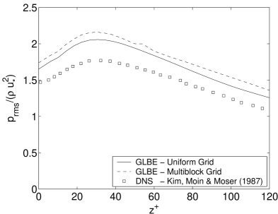
Figure 19: Root-mean-square (rms) pressure fluctuations normalized by the wall shear stress for fully-developed turbulent channel flow at $\mathrm{Re}_{*}=183.6$. Lines are GLBE results on locally refined multiblock (broken) and uniform (solid) grids, and symbols are Kim, Moin and Moser’s DNS data (1987) Kim et al. (1987).

V.3 Parallel Scalability

One of the main advantages of the LBM is its natural amenability for implementation on parallel computers. The code implementation of GLBE with forcing term was parallelized using the Message Passing Interface library through a domain decomposition strategy that exploits the local and explicit nature of the approach. It was tested for parallel scalability on a large parallel cluster known as Seaborg located at U.S. Department of Energy’s NERSC center. In these tests, the size of each subdomain was held constant at $20\times 256\times 256$ ($1.3$ million grid nodes), per processor for wall-bounded turbulence simulations. The speed-up factors obtained for up to 1024 processors are shown in Fig. 20.

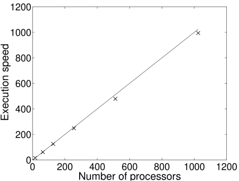
Figure 20: Parallel scalability of GLBE for turbulence simulation on a parallel cluster, Seaborg, at Department of Energy’s NERSC. Symbols are GLBE performance and line is the ideal linear speed-up.

It is evident that near-linear scaling can be obtained on massively parallel clusters and thus it appears that the GLBE approach is well-suited for large-scale turbulent flow simulations.

VI Three-Dimensional Flow in a Cubical Cavity

Let us now consider another wall-bounded flow problem, viz., 3D flow in a cubical cavity driven by its top lid, and its computation using the GLBE. Although the geometry is simple, it is characterized by richness in fluid flow physics as there are no homogeneous directions and the presence of walls on all sides profoundly modifies the flow behavior. Features such as multiple counter-rotating recirculating regions at the corners, Taylor–Görtler-type vortices, bifurcations in flows and transition to turbulence may manifest themselves depending on the Reynolds number Shankar and Deshpande (2000). Generally, when the Reynolds number $\mathrm{Re}$ based on the cavity side length is less than 2000, the flow field is laminar, and flow instabilities manifest themselves near the downstream corner eddy when $\mathrm{Re}$ is between 2000 and 3000. As $\mathrm{Re}$ increases, turbulence is generated near the cavity walls, with the flow near the downstream corner eddy becoming fully turbulent when $\mathrm{Re}{\lower 5.0pt\hbox{$>$}\atop\raise 1.0pt\hbox{$\sim$}}10,000$. Due to various states exhibited by the flow at higher $\mathrm{Re}$ it is a very challenging problem to study, in particular in obtaining computational results as it requires accurate methods with long averaging times. Measurements from experiments in cubical cavity are available for $\mathrm{Re}=10,000$ in Prasad and Koseff Prasad and Koseff (1989), while pseudo-spectral DNS and spectral element LES were performed more recently at $\mathrm{Re}=12,000$ by Leriche and Gavrilakis Leriche and Gavrilakis (2000) and Bouffanais et al. Bouffanais et al. (2007), respectively. In the context of LBM, d’Humières et al. d‘Humières et al. (2002) performed simulations of 3D flow in a diagonally driven cavity, in the laminar and transition regime, i.e. $\mathrm{Re}\leq 4000$. The focus here is to perform GLBE simulations at a higher $\mathrm{Re}$ of $12,000$ and compare results with available prior computational results Leriche and Gavrilakis (2000); Bouffanais et al. (2007) and experimental data Prasad and Koseff (1989). In addition, we also compare numerical stability of the GLBE and the SRT-LBE for this problem at higher $\mathrm{Re}$ range.

The computational conditions that we considered are as follows. The schematic of the 3D flow in a cubic cavity of side length $2W$ is shown in Fig. 21 with a coordinate system, in which flow is driven by the top lid with velocity $U_{0}$.

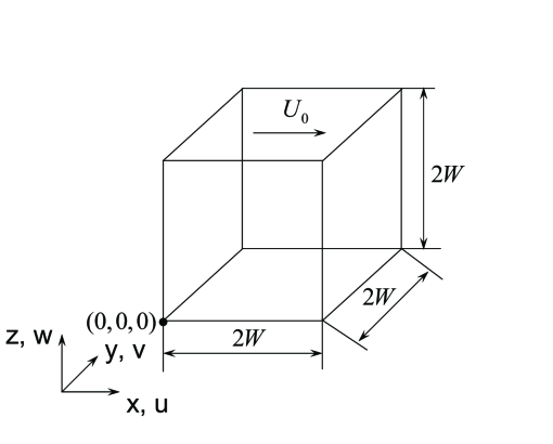
Figure 21: Schematic arrangement of computational domain for LES of flow in a three-dimensional cubical cavity of half-width $W$ driven by its top lid with velocity $U_{0}$.

The Reynolds number used in our computations $\mathrm{Re}=U_{0}2W/\nu_{0}=12,000$ is achieved by setting the lid velocity to be $U_{0}=0.12$, with a viscosity of $\nu_{0}=0.00128$ on a relatively fine uniform grid with $128^{3}$ lattice nodes. A note regarding the choice of the lid velocity is in order. For a given $\mathrm{Re}$, when the fluid viscosity is chosen based on relaxation parameter so as to maintain numerical stability, the choice of $U_{0}$ influences the number of grid nodes needed to resolve each side of the 3D cubic cavity. That is, any reduction of $U_{0}$ by a factor $k$ will increase the total number of grid nodes by $k^{3}$. On the other hand, since the GLBE is a weakly compressible computational approach, the Mach number $\mathrm{Ma}$ ($=U_{0}/c_{s}$ where $c_{s}=1/\sqrt{3}$) should be small. Thus, the value of $U_{0}$ is chosen as a compromise between satisfying the weakly compressible condition and resolution requirements so as the obtain an acceptable level of solution accuracy. In this work, as found later, the choice of $U_{0}=0.12$ and a resolution with $128^{3}$ grid nodes yields reasonably good accuracy.

Now, imposing a constant lid velocity profile on the top lid leads to edge and corner singularities and can significantly affect the stability, convergence and accuracy of simulations at such high $\mathrm{Re}$ Leriche and Gavrilakis (2000); Bouffanais et al. (2007). In reality, there is a velocity distribution at the top lid, whose precise form is not known. Following Leriche and Gavrilakis Leriche and Gavrilakis (2000) as well as Bouffanais et al. Bouffanais et al. (2007), we set the following velocity profile for the lid:

$$u_{lid}(x,y)=u_{0}\left[1-\left(\frac{x-W}{W}\right)^{18}\right]^{2}\left[1-\left(\frac{y-W}{W}\right)^{18}\right]^{2}.$$ (17)

It was found that the flow field in the cavity is not overly sensitive to the lid velocity profile, when such higher-order polynomial distributions are used Leriche and Gavrilakis (2000); Bouffanais et al. (2007). The mean value of this velocity profile is $U_{m}\approx 0.85U_{0}$, with over $75\%$ area of the lid has a velocity above $U_{m}$ and the corresponding Reynolds number on the mean velocity is $10,200$. In the GLBE, the velocity boundary condition at the lid is provided by setting the distribution function of incoming populations corresponding to $\overrightarrow{e}_{\overline{\alpha}}$ through an momentum-augmented bounce back as follows Bouzidi et al. (2001):

$$f_{\overline{\alpha}}=f_{\alpha}+2w_{\alpha}\rho_{0}\frac{\overrightarrow{e_{\overline{\alpha}}}\cdot\overrightarrow{u}_{lid}}{c_{s}^{2}}$$ (18)

where $\overrightarrow{e}_{\overline{\alpha}}=-\overrightarrow{e}_{\alpha}$. No-slip zero velocity boundary conditions based on bounce back approach are set for all the other walls. A statistically stationary state of the flow field is obtained after running for $500T^{*}$ and then collecting statistics at each grid node averaged over a period of $150T^{*}$, where the characteristic time is $T^{*}=2W/u_{0}$.

Figures 22 and 23 show the computed first-order statistics, viz., the mean velocity profile on two of the cavity centerlines along with the other available data for comparison.

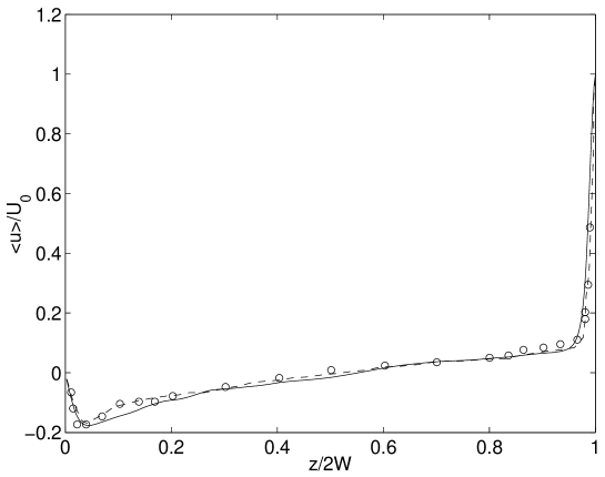
Figure 22: Mean velocity $<u>$ on the centerline $x=W,y=W$ obtained in LES using GLBE (solid line) compared with DNS of Leriche and Gavrilakis (2000) Leriche and Gavrilakis (2000) (dashed line) and experimental data of Prasad and Koseff (1989) Prasad and Koseff (1989) (circles).

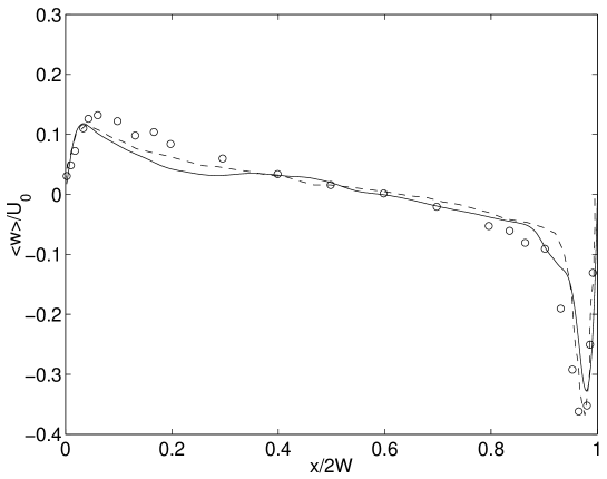
Figure 23: Mean velocity $<w>$ on the centerline $y=W,z=W$ obtained in LES using GLBE (solid line) compared with DNS of Leriche and Gavrilakis (2000) Leriche and Gavrilakis (2000) (dashed line) and experimental data of Prasad and Koseff (1989) Prasad and Koseff (1989) (circles).

It is seen that GLBE solution is in reasonable agreement with the DNS Leriche and Gavrilakis (2000) and experimental data Prasad and Koseff (1989).

In general, as discussed in Ref. Leriche and Gavrilakis (2000), momentum transfer from the lid creates a region of high pressure in the upper corner of the downstream wall as the flow has to change direction, dissipating part of its energy. The flow then convects downwards along the downstream wall like an unsteady wall jet, which separates from the wall near the mid-section of the wall and leading to two elliptical jets. They subsequently impinge on the bottom cavity wall and generate turbulence, which is convected away by the central and main vortex. The second-order statistics of the fluctuating flow field provide an indication of the turbulent activity. Figures 24 and 25 provide the rms velocity fluctuations along the direction parallel to the lid motion, i.e. $u_{rms}$ on the centerlines $y=W,z=W$ and $x=W,y=W$, respectively,

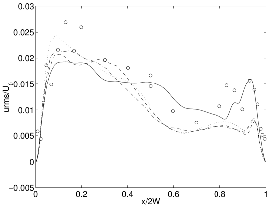
Figure 24: Root mean square (rms) velocity fluctuations $urms$ on the centerline $y=W,z=W$ obtained in LES using GLBE (solid line) compared with DNS of Leriche and Gavrilakis (2000) Leriche and Gavrilakis (2000) (dashed line), LES with NSE of Bouffanais et al. (2007) Bouffanais et al. (2007) based on dynamic model (dotted line) and dynamic mixed model (dot-dashed line) and experimental data of Prasad and Koseff (1989) Prasad and Koseff (1989) (circles).

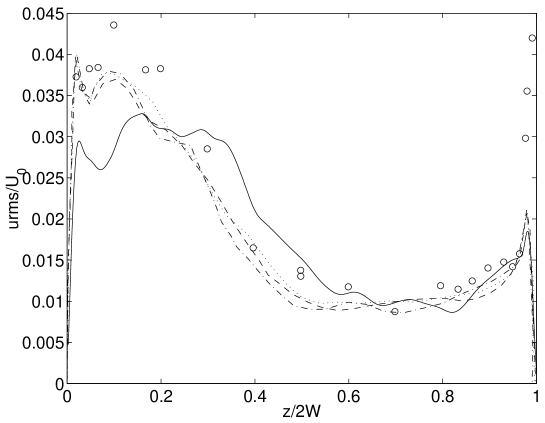
Figure 25: Root mean square (rms) velocity fluctuations $urms$ on the centerline $x=W,y=W$ obtained in LES using GLBE (solid line) compared with DNS of Leriche and Gavrilakis (2000) Leriche and Gavrilakis (2000) (dashed line), LES with NSE of Bouffanais et al. (2007) Bouffanais et al. (2007) based on dynamic model (dotted line) and dynamic mixed model (dot-dashed line) and experimental data of Prasad and Koseff (1989) Prasad and Koseff (1989) (circles).

while Figs. 26 and 27 provide the rms velocity fluctuations along direction normal to the lid motion i.e. $w_{rms}$ on the centerlines $y=W,z=W$ and $x=W,y=W$, respectively.

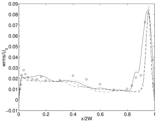
Figure 26: Root mean square (rms) velocity fluctuations $wrms$ on the centerline $y=W,z=W$ obtained in LES using GLBE (solid line) compared with DNS of Leriche and Gavrilakis (2000) Leriche and Gavrilakis (2000)(dashed line), LES with NSE of Bouffanais et al. (2007) Bouffanais et al. (2007) based on dynamic model (dotted line) and dynamic mixed model (dot-dashed line) and experimental data of Prasad and Koseff (1989) Prasad and Koseff (1989) (circles).

Figure 27: Root mean square (rms) velocity fluctuations $wrms$ on the centerline $x=W,y=W$ obtained in LES using GLBE (solid line) compared with DNS of Leriche and Gavrilakis (2000) Leriche and Gavrilakis (2000)(dashed line), LES with NSE of Bouffanais et al. (2007) Bouffanais et al. (2007) based on dynamic model (dotted line) and dynamic mixed model (dot-dashed line) and experimental data of Prasad and Koseff (1989) Prasad and Koseff (1989) (circles).

In addition, the components of the Reynolds stress $<u^{\prime}w^{\prime}>$ on the centerlines $y=W,z=W$ and $x=W,y=W$ are provided in Figs. 28 and 29, respectively.

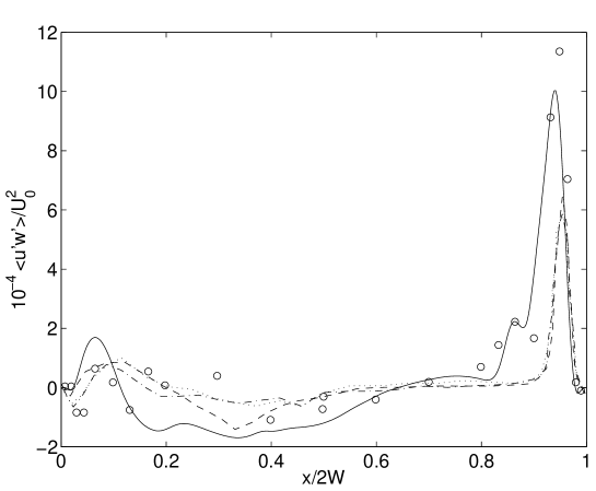
Figure 28: Reynolds stress $<u^{\prime}w^{\prime}>$ on the centerline $y=W,z=W$ obtained in LES using GLBE (solid line) compared with DNS of Leriche and Gavrilakis (2000) Leriche and Gavrilakis (2000) (dashed line), LES with NSE of Bouffanais et al. (2007) Bouffanais et al. (2007) based on dynamic model (dotted line) and dynamic mixed model (dot-dashed line) and experimental data of Prasad and Koseff (1989) Prasad and Koseff (1989) (circles).

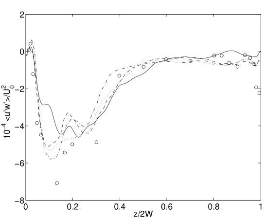
Figure 29: Reynolds stress $<u^{\prime}w^{\prime}>$ on the centerline $x=W,y=W$ obtained in LES using GLBE (solid line) compared with DNS of Leriche and Gavrilakis (2000) Leriche and Gavrilakis (2000) (dashed line), LES with NSE of Bouffanais et al. (2007) Bouffanais et al. (2007) based on dynamic model (dotted line) and dynamic mixed model (dot-dashed line) and experimental data of Prasad and Koseff (1989) Prasad and Koseff (1989) (circles).

Firstly, these results indeed show that turbulence is generated along cavity walls. In particular, the turbulent fluctuations are about an order of magnitude larger near the downstream wall than near the upstream wall. Moreover, the fluctuations are the largest along the bottom wall. These seem to be consistent with the description of the features of the fluid motion in the cavity, as elucidated in the DNS Leriche and Gavrilakis (2000). Although there is some deviation in the peaks of the fluctuations when compared with other data, considering that DNS and LES considered here are based on approaches using higher-order spectral methods Leriche and Gavrilakis (2000); Bouffanais et al. (2007), the GLBE computations, in general, compare reasonably well with them, which are very encouraging.

Some differences observed between computed solutions, including those from DNS and LES Leriche and Gavrilakis (2000); Bouffanais et al. (2007), and the experimental data could be attributed to differences in Reynolds number as well as the averaging times used. For example, the magnitude of the peak value of the near-wall Reynolds stress in Fig. 28 is influenced by the length of the time interval over which averaging is performed. In this work, we have chosen the time period of averaging ($150T^{*}$) from the sampling period used in experiments Prasad and Koseff (1989). In effect, our results are closer to these data. However, it should be noted that prior computations Leriche and Gavrilakis (2000); Bouffanais et al. (2007) found that the peak value of Reynolds stress is conditioned by rare events, which occur on time intervals of approximately $80T^{*}$. Hence, the averaging period in Refs. Leriche and Gavrilakis (2000); Bouffanais et al. (2007) is chosen such that the rare events, which tend to suppress fluctuations, are sampled many times, which accounts for the difference between experiments Prasad and Koseff (1989) (including this work) and prior computations Leriche and Gavrilakis (2000); Bouffanais et al. (2007).

Moreover, a note regarding the influence of the choice of the SGS turbulence model on the turbulence statistics results is in order. Bouffanais et al. Bouffanais et al. (2007), who employed dynamic SGS models in their computations yielding high fidelity results in excellent agreement with DNS, also reported preliminary results without employing a SGS model, i.e. unresolved DNS, and with a constant Smagorinsky SGS model. They found that the unresolved DNS is not even qualitatively correct for this problem and the use of constant Smagorinsky SGS model resulted in improved predictions, but still not fully consistent with the resolved DNS and their results with using dynamic models. However, unlike Bouffanais et al. Bouffanais et al. (2007), in this work, we have used van Driest wall damping function van Driest (1956) in conjunction with the constant Smagorinsky SGS model, which appears to make considerable difference in further improving the quality of the results. It appears that the use of wall damping function, which accounts for reduction of near-wall turbulent length scales, yields results that are significantly closer and more consistent than without the use of such a damping function. This is also consistent with our recent observation Premnath et al. (2008) that the use of a wall damping function with constant Smagorinsky SGS model results in better agreement with the dynamic SGS model results for LES of turbulent channel flow than without it. It should, however, also be noted that while the results obtained with the use of damping function are generally better, they are in some cases somewhat underpredicted near walls, e.g. Fig. 25, and the peaks in some other cases are broader, e.g. Fig. 26. While the motivation for the use of damping function is simplicity and computational efficiency, it is, of course, desirable to employ dynamic SGS models in the LBM framework Premnath et al. (2008) for further improvements.

VI.1 Numerical Stability

We will now make direct comparisons of stability characteristics of the GLBE with the SRT-LBE for 3D cavity flow simulations at higher Reynolds number ranges, complementing an earlier study d‘Humières et al. (2002). In both approaches, for a given grid resolution, the shear viscosity was fixed and the lid velocity was increased gradually until the computation became unstable. Figure 30 shows the maximum Reynolds number that could be attained before the computations became unstable. Results are provided for different grid resolutions and viscosities for both the approaches.

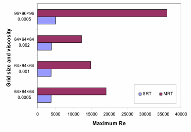
Figure 30: (Color online) Comparison of numerical stability characteristics of GLBE with SRT-LBE for 3D cavity flows: Maximum attainable Reynolds number for a given resolution and shear viscosity.

The superior stability characteristics of the GLBE are evident for this wall-bounded turbulent flow problem. The GLBE computations can reach Reynolds numbers that are several times higher than that of the SRT-LBE, typically by a factor of $3$ or $4$ and sometimes even about as high as an order magnitude. Indeed, the SRT-LBE became unstable and unable to simulate the $\mathrm{Re}=12,000$ case considered above with a resolution of $128^{3}$ using the GLBE.

VII Summary and Conclusions

A generalized lattice Boltzmann equation (GLBE) with forcing term, which uses multiple relaxation times, for eddy-capturing computations of wall-bounded turbulent flows that are characterized by statistical anisotropy and inhomogeneity is discussed. Standard Smagorinsky eddy viscosity model is used to represent SGS turbulence effects, which is modified by the van Driest damping function to account for reduction of turbulent length scales near walls. Second-order and effectively time-explicit source terms, which represent general forms of non-uniform external forces that drive or modulate the character of turbulent flow, are projected onto the natural moment space of GLBE in this formulation. In this framework, the strain tensor used in the SGS model is related to the non-equilibrium moments and the forcing terms in moment space. Furthermore, local grid refinement using a conservative multiblock approach is used to coarsen grids in the bulk flow region, where turbulent dissipation or Kolmogorov length scales become larger. Computational optimization, particularly in the presence of moment-projections of the forcing terms, is also discussed.

Two canonical bounded flows, viz., fully-developed turbulent channel flow and 3D driven cavity flow have been simulated using this approach for shear Reynolds number of $183.6$ and Reynolds number based on cavity side length of $12,000$ respectively. The structure of turbulent flow given in terms of turbulence statistics, including mean velocity and components of root-mean-square (rms) velocity and vorticity fluctuations and Reynolds stress are in good agreement with prior DNS and experimental data. The computed rms pressure fluctuations are found to be somewhat over-predicted in comparison with DNS data, which is based on the solution of incompressible Navier–Stokes equations. It is thought this may due to the kinetic nature of the GLBE approach, which is inherently weakly compressible. In the case of 3D cavity flow, the GLBE is able to capture turbulent velocity fluctuations and Reynolds stresses generated by cavity walls, which are in reasonably good agreement with prior data.

With regard to numerical stability, it is found that by separating various relaxation times, the GLBE is able to maintain solution fidelity, while the SRT-LBE solution can exhibit spurious effects on velocity fluctuations in the near-wall region, particularly in the wall normal component, on relatively coarser grids in turbulent channel flow simulations. The GLBE is found to be superior in maintaining numerical stability at higher Reynolds number $\mathrm{Re}$ for 3D cavity flows, with the maximum attainable $\mathrm{Re}$ several times that for the SRT-LBE, depending on the resolution and shear viscosity of the fluid. Moreover, parallel implementation of the GLBE approach is able to maintain near-linear scalability in performance for over a thousand processors on a large parallel cluster.

The GLBE with forcing term appears to be a reliable approach for LES of wall-bounded turbulent flows. It is expected that further improvements can be achieved by introducing more advanced SGS models based on dynamic procedures Germano et al. (1991); Zang et al. (1993); Salvetti and Banerjee (1995) in the LBM Premnath et al. (2008).

Appendix A Components of Moments, Equilibrium Moments and Moment-Projections of Forcing Terms for the D3Q19 Lattice

The components of the various elements in the moments are as follows d‘Humières et al. (2002): $\widehat{f}_{0}=\rho,\widehat{f}_{1}=e,\widehat{f}_{2}=e^{2},\widehat{f}_{3}=j_{x},\widehat{f}_{4}=q_{x},\widehat{f}_{5}=j_{y},\widehat{f}_{6}=q_{y},\widehat{f}_{7}=j_{z},\widehat{f}_{8}=q_{z},\widehat{f}_{9}=3p_{xx},\widehat{f}_{10}=3\pi_{xx},\widehat{f}_{11}=p_{ww},\widehat{f}_{12}=\pi_{ww},\widehat{f}_{13}=p_{xy},\widehat{f}_{14}=p_{yz},\widehat{f}_{15}=p_{xz},\widehat{f}_{16}=m_{x},\widehat{f}_{17}=m_{y},\widehat{f}_{18}=m_{z}$.

Here, $\rho$ is the density, $e$ and $e^{2}$ represent kinetic energy that is independent of density and square of energy, respectively; $j_{x}$, $j_{y}$ and $j_{z}$ are the components of the momentum, i.e. $j_{x}=\rho u_{x}$, $j_{y}=\rho u_{y}$, $j_{z}=\rho u_{z}$, $q_{x}$, $q_{y}$, $q_{z}$ are the components of the energy flux, and $p_{xx}$, $p_{xy}$, $p_{yz}$ and $p_{xz}$ are the components of the symmetric traceless viscous stress tensor. The other two normal components of the viscous stress tensor, $p_{yy}$ and $p_{zz}$, can be constructed from $p_{xx}$ and $p_{ww}$, where $p_{ww}=p_{yy}-p_{zz}$. Other moments include $\pi_{xx}$, $\pi_{ww}$, $m_{x}$, $m_{y}$ and $m_{z}$. The first two of these moments have the same symmetry as the diagonal part of the traceless viscous tensor $p_{ij}$, while the last three vectors are parts of a third rank tensor, with the symmetry of $j_{k}p_{mn}$.

The components of the equilibrium moments for the D3Q19 lattice are as follows: d‘Humières et al. (2002): $\widehat{f}_{0}^{eq}=\rho,\widehat{f}_{1}^{eq}\equiv e^{eq}=-11\rho+19\frac{\overrightarrow{j}\cdot\overrightarrow{j}}{\rho},\widehat{f}_{2}^{eq}\equiv e^{2,eq}=3\rho-\frac{11}{2}\frac{\overrightarrow{j}\cdot\overrightarrow{j}}{\rho},\widehat{f}_{3}^{eq}=j_{x},\widehat{f}_{4}^{eq}\equiv q_{x}^{eq}=-\frac{2}{3}j_{x},\widehat{f}_{5}^{eq}=j_{y},\widehat{f}_{6}^{eq}\equiv q_{y}^{eq}=-\frac{2}{3}j_{y},\widehat{f}_{7}^{eq}=j_{z},\widehat{f}_{8}^{eq}\equiv q_{z}^{eq}=-\frac{2}{3}j_{z},\widehat{f}_{9}^{eq}\equiv 3p_{xx}^{eq}=\frac{\left[3j_{x}^{2}-\overrightarrow{j}\cdot\overrightarrow{j}\right]}{\rho},\widehat{f}_{10}^{eq}\equiv 3\pi_{xx}^{eq}=3\left(-\frac{1}{2}p_{xx}^{eq}\right),\widehat{f}_{11}^{eq}\equiv p_{ww}^{eq}=\frac{\left[j_{y}^{2}-j_{z}^{2}\right]}{\rho},\widehat{f}_{12}^{eq}\equiv\pi_{ww}^{eq}=-\frac{1}{2}p_{ww}^{eq},\widehat{f}_{13}^{eq}\equiv p_{xy}^{eq}=\frac{j_{x}j_{y}}{\rho},\widehat{f}_{14}^{eq}\equiv p_{yz}^{eq}=\frac{j_{y}j_{z}}{\rho},\widehat{f}_{15}^{eq}\equiv p_{xz}^{eq}=\frac{j_{x}j_{z}}{\rho},\widehat{f}_{16}^{eq}=0,\widehat{f}_{17}^{eq}=0,\widehat{f}_{18}^{eq}=0$.

The components of the source terms in moment space can be obtained by multiplying the transformation matrix with Eq. (5). The final expressions are as follows:

$\widehat{S}_{0}=0,\qquad\widehat{S}_{1}=38(F_{x}u_{x}+F_{y}u_{y}+F_{z}u_{z}),\qquad\widehat{S}_{2}=-11(F_{x}u_{x}+F_{y}u_{y}+F_{z}u_{z}),$

$\widehat{S}_{3}=F_{x},\qquad\widehat{S}_{4}=-\frac{2}{3}F_{x},\qquad\widehat{S}_{5}=F_{y},\qquad\widehat{S}_{6}=-\frac{2}{3}F_{y},\qquad\widehat{S}_{7}=F_{z},\qquad\widehat{S}_{8}=-\frac{2}{3}F_{z},$

$\widehat{S}_{9}=2(2F_{x}u_{x}-F_{y}u_{y}-F_{z}u_{z}),\qquad\widehat{S}_{10}=-(2F_{x}u_{x}-F_{y}u_{y}-F_{z}u_{z}),$

$\widehat{S}_{11}=2(F_{y}u_{y}-F_{z}u_{z}),\qquad\widehat{S}_{12}=-(F_{y}u_{y}-F_{z}u_{z}),\qquad\widehat{S}_{13}=(F_{x}u_{y}+F_{y}u_{x}),$

$\widehat{S}_{14}=(F_{y}u_{z}+F_{z}u_{y}),\qquad\widehat{S}_{15}=(F_{x}u_{z}+F_{z}u_{x}),\qquad\widehat{S}_{16}=0,\qquad\widehat{S}_{17}=0,\qquad\widehat{S}_{18}=0$.

The self-consistency of the moment projections of source terms is evident. For e.g., $\widehat{S}_{3}$, $\widehat{S}_{5}$ and $\widehat{S}_{7}$ provide Cartesian components of body forces on the moments corresponding to the components of momentum (mass flux), $\widehat{S}_{1}$ provides the work due to forces on the moment corresponding to kinetic energy, etc.

Appendix B Strain Rate Tensor using Non-equilibrium Moments in the GLBE with Forcing Term

In this section, we will present a brief derivation of the strain rate tensor in terms of the non-equilibrium moments of the GLBE with forcing term by applying a Chapman–Enskog analysis. The results that follow are generalizations of those presented by Yu et al. Yu et al. (2006) to include forcing terms representing non-uniform forces. First, the left hand side of the GLBE is simplified by applying Taylor series, which results in the following:

$$\delta_{t}\mathbb{D}_{t}\mathbf{\widehat{f}}\approx-\mathcal{T}^{-1}\widehat{\Lambda}\left(\mathbf{\widehat{f}}-\mathbf{\widehat{f}}^{eq}\right)+\mathcal{T}^{-1}\left(\mathrm{I}-\frac{1}{2}\widehat{\Lambda}\right)\mathbf{\widehat{S}}\delta_{t},$$ (19)

where $\mathbb{D}_{t}=diag\left(\partial_{t_{0}},\partial_{t_{0}}+\overrightarrow{e_{1}}\cdot\overrightarrow{\nabla},\ldots,\partial_{t_{0}}+\overrightarrow{e_{18}}\cdot\overrightarrow{\nabla}\right)$. Now applying the Chapman–Enskog expansion

$$\widehat{\mathbf{f}}\approx\widehat{\mathbf{f}}^{eq}+\widehat{\mathbf{f}}^{(1)}\delta_{t}$$ (20)

to Eq. (19), and truncating terms of order $O(\delta_{t}^{2})$ or higher, we get

$$\widehat{\mathbb{D}_{t}}\widehat{\mathbf{f}}^{eq}=-\widehat{\Lambda}\widehat{\mathbf{f}}^{(1)}+\left(\mathrm{I}-\frac{1}{2}\widehat{\Lambda}\right)\widehat{\mathbf{S}},$$ (21)

where $\widehat{\mathbb{D}_{t}}=\mathcal{T}\mathbb{D}_{t}\mathcal{T}^{-1}=diag\left(\partial_{t_{0}},\partial_{t_{0}}+\widehat{\Xi}_{1i}\partial_{i},\ldots,\partial_{t_{0}}+\widehat{\Xi}_{18i}\partial_{i}\right)$, in which and henceforth summation of repeated indices is assumed. Eq. (21) can be rewritten in terms of non-equilibrium moments $\widehat{\mathbf{f}}^{(1)}$ as

$$\widehat{\mathbf{f}}^{(1)}\approx-\widehat{\Lambda}^{-1}\left(\partial_{t_{0}}+\widehat{\Xi}_{1i}\partial_{i}\right)\widehat{\mathbf{f}}^{eq}+\left(\widehat{\Lambda}-\frac{1}{2}\mathrm{I}\right)\widehat{\mathbf{S}},$$ (22)

where $\widehat{\Xi}_{\alpha i}=\mathcal{T}e_{\alpha i}\mathcal{T}^{-1}$.

Now substituting the expressions for the equilibrium moments $\widehat{\mathbf{f}}^{eq}$ and the source terms $\widehat{\mathbf{S}}$ in Eq. (22), we simplify the expressions for the components of the non-equilibrium moments. Some such components of interest are as follows:

$$\widehat{f}^{(1)}_{1}\equiv e^{(1)}=-\frac{1}{s_{1}}\left\{\partial_{t_{0}}\left(-11\rho+19\frac{j_{k}j_{k}}{\rho}\right)+\frac{5}{3}\partial_{k}j_{k}\right\}+\left(\frac{1}{s_{1}}-\frac{1}{2}\right)\widehat{S}_{1},$$ (23)

$$\widehat{f}^{(1)}_{9}\equiv 3p_{xx}^{(1)}=-\frac{1}{s_{9}}\left\{\partial_{t_{0}}\left(\frac{j_{y}^{2}-j_{z}^{2}}{\rho}\right)+\frac{2}{3}\left(2\partial_{x}j_{x}-\partial_{y}j_{y}-\partial_{z}j_{z}\right)\right\}+\left(\frac{1}{s_{9}}-\frac{1}{2}\right)\widehat{S}_{9},$$ (24)

$$\widehat{f}^{(1)}_{11}\equiv p_{ww}^{(1)}=-\frac{1}{s_{11}}\left\{\partial_{t_{0}}\left(\frac{j_{y}^{2}-j_{z}^{2}}{\rho}\right)+\frac{2}{3}\left(\partial_{y}j_{y}-\partial_{z}j_{z}\right)\right\}+\left(\frac{1}{s_{11}}-\frac{1}{2}\right)\widehat{S}_{11},$$ (25)

$$\widehat{f}^{(1)}_{13}\equiv p_{xy}^{(1)}=-\frac{1}{s_{13}}\left\{\partial_{t_{0}}\left(\frac{j_{x}j_{y}}{\rho}\right)+\frac{1}{3}\left(\partial_{x}j_{y}+\partial_{y}j_{x}\right)\right\}+\left(\frac{1}{s_{13}}-\frac{1}{2}\right)\widehat{S}_{13},$$ (26)

$$\widehat{f}^{(1)}_{14}\equiv p_{yz}^{(1)}=-\frac{1}{s_{14}}\left\{\partial_{t_{0}}\left(\frac{j_{y}j_{z}}{\rho}\right)+\frac{1}{3}\left(\partial_{y}j_{z}+\partial_{z}j_{y}\right)\right\}+\left(\frac{1}{s_{14}}-\frac{1}{2}\right)\widehat{S}_{14},$$ (27)

$$\widehat{f}^{(1)}_{15}\equiv p_{xz}^{(1)}=-\frac{1}{s_{15}}\left\{\partial_{t_{0}}\left(\frac{j_{x}j_{z}}{\rho}\right)+\frac{1}{3}\left(\partial_{x}j_{z}+\partial_{z}j_{x}\right)\right\}+\left(\frac{1}{s_{15}}-\frac{1}{2}\right)\widehat{S}_{15}.$$ (28)

.

For further simplification, we invoke the following approximations: $\partial_{t_{0}}\left(\frac{j_{x}^{2}}{\rho}\right)\simeq 2u_{x}F_{x},\quad\partial_{t_{0}}\left(\frac{j_{y}^{2}}{\rho}\right)\simeq 2u_{y}F_{y},\quad\partial_{t_{0}}\left(\frac{j_{z}^{2}}{\rho}\right)\simeq 2u_{z}F_{z},$ $\partial_{t_{0}}\left(\frac{j_{x}j_{y}}{\rho}\right)\simeq u_{x}F_{y}+u_{y}F_{x},\quad\partial_{t_{0}}\left(\frac{j_{y}j_{z}}{\rho}\right)\simeq u_{y}F_{z}+u_{z}F_{y},\quad\partial_{t_{0}}\left(\frac{j_{x}j_{z}}{\rho}\right)\simeq u_{x}F_{z}+u_{z}F_{x},$ and $\partial_{t_{0}}\rho=-\partial_{k}j_{k},$ which result in

$$\widehat{f}^{(1)}_{1}=-\frac{38}{3}\frac{1}{s_{1}}\partial_{k}j_{k}-\frac{1}{2}\widehat{S}_{1},$$ (29)

$$\widehat{f}^{(1)}_{9}\approx-\frac{2}{3}\frac{1}{s_{9}}\left(3\partial_{x}j_{x}-\partial_{k}j_{k}\right)-\frac{1}{2}\widehat{S}_{9},$$ (30)

$$\widehat{f}^{(1)}_{11}\approx-\frac{2}{3}\frac{1}{s_{11}}\left(\partial_{y}j_{y}-\partial_{z}j_{z}\right)-\frac{1}{2}\widehat{S}_{11},$$ (31)

$$\widehat{f}^{(1)}_{13}\approx-\frac{1}{3}\frac{1}{s_{13}}\left(\partial_{x}j_{y}+\partial_{y}j_{x}\right)-\frac{1}{2}\widehat{S}_{13},$$ (32)

$$\widehat{f}^{(1)}_{14}\approx-\frac{1}{3}\frac{1}{s_{14}}\left(\partial_{y}j_{z}+\partial_{z}j_{y}\right)-\frac{1}{2}\widehat{S}_{14},$$ (33)

$$\widehat{f}^{(1)}_{15}\approx-\frac{1}{3}\frac{1}{s_{15}}\left(\partial_{x}j_{z}+\partial_{z}j_{x}\right)-\frac{1}{2}\widehat{S}_{15}.$$ (34)

It follows from the above that the components of the strain rate tensor can be written explicitly in terms of non-equilibrium moments as

$$S_{xx} \approx -\frac{1}{38\rho}\left[s_{1}\widehat{h}_{1}^{(neq)}+19s_{9}\widehat{h}_{9}^{(neq)}\right],$$ (35)

$$S_{yy} \approx -\frac{1}{76\rho}\left[2s_{1}\widehat{h}_{1}^{(neq)}-19\left(s_{9}\widehat{h}_{9}^{(neq)}-3s_{11}\widehat{h}_{11}^{(neq)}\right)\right],$$ (36)

$$S_{zz} \approx -\frac{1}{76\rho}\left[2s_{1}\widehat{h}_{1}^{(neq)}-19\left(s_{9}\widehat{h}_{9}^{(neq)}+3s_{11}\widehat{h}_{11}^{(neq)}\right)\right],$$ (37)

$$S_{xy} \approx -\frac{3}{2\rho}s_{13}\widehat{h}_{13}^{(neq)},$$ (38)

$$S_{yz} \approx -\frac{3}{2\rho}s_{14}\widehat{h}_{14}^{(neq)},$$ (39)

$$S_{xz} \approx -\frac{3}{2\rho}s_{15}\widehat{h}_{15}^{(neq)},$$ (40)

where

$$\widehat{h}_{\alpha}^{(neq)}=\widehat{f}_{\alpha}-\widehat{f}_{\alpha}^{eq}+\frac{1}{2}\widehat{S}_{\alpha},\qquad\alpha\in\{1,9,11,13,14,15\}$$ (41)

Here, the components of the source term $\widehat{S}_{\alpha}$ can be obtained from Appendix A. The form of $S_{ij}$ turns out to be very similar to that obtained by Yu et al. Yu et al. (2006), except for the expression ${h}_{\alpha}^{(neq)}$, which contains the additional contribution $\frac{1}{2}\widehat{S}_{\alpha}$ that provides the effect of the forcing term. The procedure discussed here, however, is general, and can be readily employed for deriving the expressions for strain rate tensor for other lattice velocity models in the presence of forcing terms. The magnitude of the strain rate $|S|$ used in turbulence models can then be obtained from Eqs. (35)–(40) as $|S|=\sqrt{2S_{ij}S_{ij}}=\sqrt{2(S_{xx}^{2}+S_{yy}^{2}+S_{zz}^{2}+2(S_{xy}^{2}+S_{yz}^{2}+S_{xz}^{2}))}$. To clarify the notations employed, we again note that $\widehat{S}_{\alpha}$ represents the source terms in moment space, $s_{\alpha}$ corresponds to the relaxation times in the collision term, and $S_{ij}$ is the strain rate tensor.

References

- Chen and Doolen (1998) S. Chen and G. Doolen, Ann. Rev. Fluid Mech. 8, 2527 (1998).
- Succi (2001) S. Succi, The Lattice Boltzmann Equation for Fluid Dynamics and Beyond (Clarendon Press, Oxford, 2001).
- Succi et al. (2002) S. Succi, I. Karlin, and H. Chen, Rev. Mod. Phys. 74, 1203 (2002).
- Yu et al. (2003) D. Yu, R. Mei, L.-S. Luo, and W. Shyy, Prog. Aero. Sci. 39, 329 (2003).
- McNamara and Zanetti (1988) G. McNamara and G. Zanetti, Phys. Rev. Lett. 61, 2332 (1988).
- Higuera and Jiménez (1989) F. Higuera and J. Jiménez, Europhys. Lett. 9, 663 (1989).
- Higuera et al. (1989) F. Higuera, S. Succi, and R. Benzi, Europhys. Lett. 9, 345 (1989).
- Qian et al. (1992) Y. Qian, D. d’Humières, and P. Lallemand, Europhys. Lett. 17, 479 (1992).
- Chen et al. (1992) H. Chen, S. Chen, and W. Matthaeus, Phys. Rev. A 45, 5339 (1992).
- Frisch et al. (1986) U. Frisch, B. Hasslacher, and Y. Pomeau, Phys. Rev. Lett. 56, 1505 (1986).
- He and Luo (1997a) X. He and L.-S. Luo, Phys. Rev. E 55, R63333 (1997a).
- He and Luo (1997b) X. He and L.-S. Luo, Phys. Rev. E 56, 6811 (1997b).
- He and Doolen (2002) X. He and G. Doolen, J. Stat. Phys. 107, 309 (2002).
- Junk et al. (2005) M. Junk, A. Klar, and L.-S. Luo, J. Comput. Phys. 210, 676 (2005).
- Nourgaliev et al. (2003) R. Nourgaliev, T. Dinh, T. Theofanous, and D. Joseph, Int. J. Multiphase Flow 29, 117 (2003).
- Frisch (1995) U. Frisch, Turbulence: The Legacy of A.N. Kolmogorov (Cambridge University Press, New York, 1995).
- Pope (2000) S. Pope, Turbulent Flows (Cambridge University Press, New York, 2000).
- Chen et al. (1998) H. Chen, S. Succi, and S. Orszag, Phys. Rev. E 59, R2527 (1998).
- Ansumali et al. (2004) S. Ansumali, I. Karlin, and S. Succi, Physica A 338, 379 (2004).
- Chen et al. (2004) H. Chen, S. Orszag, and I. Straroselsky, J. Fluid Mech. 519, 301 (2004).
- Teixeira (1998) C. Teixeira, Int. J. Mod. Phys. C 9, 1159 (1998).
- Chen et al. (2003) H. Chen, S. Kandasamy, S. Orszag, R. Shock, S. Succi, and V. Yakhot, Science 301, 633 (2003).
- Martinez et al. (1994) D. Martinez, W. Matthaeus, S. Chen, and D. Montgomery, Phys. Fluids 6, 1285 (1994).
- Amati et al. (1997) G. Amati, S. Succi, and R. Benzi, Fluid Dyn. Res. 19, 289 (1997).
- Amati et al. (1999) G. Amati, S. Succi, and R. Piva, Fluid Dyn. Res. 24, 201 (1999).
- Yu and Girimaji (2005) D. Yu and S. S. Girimaji, J. Turb. 6, 1 (2005).
- Yu et al. (2005a) H. Yu, S. S. Girimaji, and L.-S. Luo, Phys. Rev. E 71, 016708 (2005a).
- Yu et al. (2005b) H. Yu, S. S. Girimaji, and L.-S. Luo, J. Comput. Phys. 209, 599 (2005b).
- Yu and Girimaji (2006) D. Yu and S. S. Girimaji, J. Fluid Mech. 566, 117 (2006).
- Lammers et al. (2006) P. Lammers, K. Beronov, R. Volkert, G. Brenner, and F. Durst, Comput. Fluids 35, 1137 (2006).
- Sagaut (2002) P. Sagaut, Large Eddy Simulation for Incompressible Flows – An Introduction (Springer, New York, 2002).
- Smagorinsky (1963) J. Smagorinsky, Monthly Weather Rev. 91, 99 (1963).
- Hou et al. (1996) S. Hou, J. Sterling, S. Chen, and G. Doolen, Fields Inst. Comm. 6, 151 (1996).
- Eggels (1996) J. Eggels, Int. J. Heat and Fluid Flow 17, 307 (1996).
- Derksen and den Akker (1999) J. Derksen and H. V. den Akker, AIChE J. 45, 209 (1999).
- Lu et al. (2002) Z. Lu, Y. Liao, Y. Qian, J. Derksen, and K. Kontomaris, J. Comput. Phys. 181, 675 (2002).
- Krafczyk et al. (2003) M. Krafczyk, J. Tölke, and L.-S. Luo, Int. J. Mod. Phys. B 17, 33 (2003).
- Hartmann et al. (2004) H. Hartmann, J. Derksen, C. Montavon, J. Pearson, I. Hamill, and H. V. den Akker, Chem. Engg. Sci. 59, 2419 (2004).
- Bhatnagar et al. (1954) P. Bhatnagar, E. Gross, and M. Krook, Phys. Rev. 94, 511 (1954).
- Lallemand and Luo (2000) P. Lallemand and L.-S. Luo, Phys. Rev. E 61, 6546 (2000).
- Dellar (2001) P. Dellar, Phys. Rev. E 64, 031203 (2001).
- Karlin et al. (1999) I. Karlin, A. Ferrente, and H. Ottinger, Eur. Phys. Lett. 47, 182 (1999).
- Ansumali and Karlin (2002) S. Ansumali and I. Karlin, Phys. Rev. E 65, 056312 (2002).
- Ansumali and Karlin (2005) S. Ansumali and I. Karlin, Phys. Rev. Lett. 95, 260605 (2005).
- Boghosian et al. (2001) B. Boghosian, J. Yepez, P. Coveney, and A. Wagner, Proc. Roy. London, Ser. A 457, 717 (2001).
- Wong and Luo (2003) W.-A. Wong and L.-S. Luo, Phys. Rev. E 67, 051105 (2003).
- Wong and Luo (2007) W.-A. Wong and L.-S. Luo, Preprint (2007).
- d‘Humières (1992) D. d‘Humières, in Generalized Lattice Boltzmann Equations. Progress in Aeronautics and Astronautics (Eds. B.D. Shigal and D.P Weaver) (1992), p. 450.
- Benzi et al. (1992) R. Benzi, S. Succi, and M. Vergassola, Phys. Rept. 222, 145 (1992).
- Resibois and Leener (1977) P. Resibois and M. D. Leener, Classical Kinetic Theory of Fluids (John Wiley and Sons, New York, 1977).
- d‘Humières et al. (2002) D. d‘Humières, I. Ginzburg, M. Krafczyk, P. Lallemand, and L.-S. Luo, Phil. Trans. R. Soc. Lond. A 360, 437 (2002).
- Ladd (1994) A. Ladd, J. Fluid. Mech. 271, 285 (1994).
- Ginzburg and d‘Humières (2003) I. Ginzburg and D. d‘Humières, Phys. Rev. E 68, 066614 (2003).
- Ginzburg (2005) I. Ginzburg, Adv. Water Res. 28, 1171 (2005).
- Adhikari et al. (2005) R. Adhikari, K. Stratford, A. Wagner, and M. Cates, Europhys. Lett. 71, 473 (2005).
- McCracken and Abraham (2005a) M. McCracken and J. Abraham, Phys. Rev. E 71, 036701 (2005a).
- Premnath and Abraham (2007) K. N. Premnath and J. Abraham, J. Comput. Phys. 224, 539 (2007).
- Premnath and Abraham (2005) K. N. Premnath and J. Abraham, Phys. Fluids 17, 122105 (2005).
- McCracken and Abraham (2005b) M. McCracken and J. Abraham, Int. J. Mod. Phys. C 16, 1671 (2005b).
- Pattison et al. (2008) M. J. Pattison, K. N. Premnath, N. B. Morley, and M. A. Abdou, Fusion Engg. Design 83, 557 (2008).
- Yu et al. (2006) H. Yu, L.-S. Luo, and S. S. Girimaji, Comput. Fluids 35, 957 (2006).
- van Driest (1956) E. van Driest, J. Aero. Sci. 23, 1007 (1956).
- Chapman and Cowling (1964) S. Chapman and T. Cowling, Mathematical Theory of Non-Uniform Gases (Cambridge University Press, London, 1964).
- Chen et al. (2006) H. Chen, O. Filippova, J. Hoch, K. Molving, R. Shock, C. Teixeira, and R. Zhang, Physica A 362, 158 (2006).
- Rohde et al. (2006) M. Rohde, D. Kandhai, J. Derksen, and H. van den Akker, Int. J. Num. Meth. Fluids 51, 439 (2006).
- Moin and Kim (1982) P. Moin and J. Kim, J. Fluid Mech. 118, 341 (1982).
- Germano et al. (1991) M. Germano, U. Piomelli, P. Moin, and W. Cabot, Phys. Fluids A 3, 1760 (1991).
- Premnath et al. (2008) K. N. Premnath, M. J. Pattison, and S. Banerjee, Physica A, submitted (2008).
- Dong et al. (2008) Y. Dong, P. Sagaut, and S. Marié, Phys. Fluids 20, 035105 (2008).
- He et al. (1998) X. He, X. Shan, and G. Doolen, Phys. Rev. E 57, R13 (1998).
- Guo et al. (2002) Z. Guo, C. Zheng, and B. Shi, Phys. Rev. E 65, 046308 (2002).
- Sone (1990) Y. Sone, in Proceedings of a Symposium Held in Honour of Henri Cabannes, Advances in Kinetic Theory and Continuum Mechanics (Eds. R. Gatignol and J.B. Soubbaramayer) (1990), p. 19.
- Junk (2001) M. Junk, Numer. Meth. Partial Diff. Eqns. 158, 267 (2001).
- Zang et al. (1993) Y. Zang, R. Street, and J. Koseff, Phys. Fluids A 5, 3186 (1993).
- Salvetti and Banerjee (1995) M. Salvetti and S. Banerjee, Phys. Fluids 7, 2831 (1995).
- Lam (1989) K. Lam, Ph.D. thesis, University of California, Santa Barbara, CA (1989).
- Mei et al. (2006) R. Mei, L.-S. Luo, P. Lallemand, and D. d’Humières, Comput. Fluids 35, 855 (2006).
- Lam and Banerjee (1992) K. Lam and S. Banerjee, Phys. Fluids A 4, 306 (1992).
- Moin and Mahesh (1998) K. Moin and K. Mahesh, Ann. Rev. Fluid Mech. 30, 539 (1998).
- Kim et al. (1987) J. Kim, P. Moin, and R. Moser, J. Fluid Mech. 177, 133 (1987).
- Choi et al. (2000) D. Choi, D. Prasad, M. Wang, and C. Pierce, Evaluation of an industrial CFD code for LES applications, Proceedings of the Summer Program 2000 (Center for Turbulence Research, Stanford, CA, 2000).
- Gullbrand and Chow (2003) J. Gullbrand and F. Chow, J. Fluid Mech. 495, 323 (2003).
- Kreplin and Eckelmann (1979) H. Kreplin and H. Eckelmann, Phys. Fluids 28, 1233 (1979).
- Willmarth (1975) W. Willmarth, Annu. Rev. Fluid Mech. 65, 13 (1975).
- Dubief and Delcayre (2000) Y. Dubief and F. Delcayre, J. Turb. 1, 1 (2000).
- Dellar (2003) P. Dellar, J. Comput. Phys. 190, 351 (2003).
- He et al. (1996) X. He, L.-S. Luo, and M. Dembo, J. Comput. Phys. 129, 537 (1996).
- Kravchenko et al. (1996) A. Kravchenko, P. Moin, and R. Moser, J. Comput. Phys. 127, 412 (1996).
- Shankar and Deshpande (2000) P. Shankar and M. Deshpande, Ann. Rev. Fluid Mech. 32, 93 (2000).
- Prasad and Koseff (1989) A. Prasad and J. Koseff, Phys. Fluids 1, 208 (1989).
- Leriche and Gavrilakis (2000) E. Leriche and S. Gavrilakis, Phys. Fluids 12, 1363 (2000).
- Bouffanais et al. (2007) R. Bouffanais, M.O.Deville, and E. Leriche, Phys. Fluids 19, 055108 (2007).
- Bouzidi et al. (2001) M. Bouzidi, M. Firdaouss, and P. Lallemand, Phys. Fluids 13, 3452 (2001).