Photonic soliton and its relevance to radiative neutrino pair emission

ABSTRACT

We consider atomic system of $\Lambda-$type 3-level coupled to 2 mode fields, and derive an effective Maxwell-Bloch equation designed for two photon emission between two lower levels. We find axially symmetric, topologically stable soliton solutions made of condensed fields. Immediate implication of soliton formation to radiative neutrino pair emission is to enhance its rate, larger than the usual $\propto N^{2}$ factor of target number dependence, along with another merit of increasing the signal to the background photon emission.

Introduction       Superfluorescence(SF) (also called superradiance) is a phenomenon of cooperative photon emission triggered by macroscopic growth of atomic polarization and induced field [1] - [4]. The total emission rate at its maximum scales with the number of targets $N$ as $\propto N^{2}$ compared to the spontaneous decay rate $\propto N$. SF has been observed in a variety of target states, ranging from gas, solid crystals [4], to Bose-Einstein condensates [5], [6]. A simplest system of SF may be described by the Dicke model [1] of 2 levels related by E1 transition. Its initial state is excited atomic state prepared for instance by pulsed laser irradiation, with and without further triggering field. SF occurs, in the case of 3 levels, to Raman process, as well [6].

The present work has been initiated by our efforts of finding an enhancement mechanism of radiative neutrino pair emission from an atomic metastable state $|1\rangle\rightarrow|2\rangle+\gamma+\nu_{i}\nu_{j}$ ($\nu_{i}$ neutrino mass eigenstates) [7], [8], in similar ways to SF. This process is useful to determine all neutrino parameters, 3 masses and 3 mixing angles, and furthermore to distinguish the Majorana neutrino from the Dirac neutrino. After the smallest neutrino mass is experimentally determined, one may proceed to detection of relic neutrino of 1.9 K using the Pauli blocking effect [9].

After derivation of effective Maxwell-Bloch (MB) equation for related two photon emission process, $|1\rangle\rightarrow|2\rangle+\gamma+\gamma$, we realized that non-trivial soliton solutions do exist, their stability being assured by the topological winding number associated with SO(2) rotation of fields. With formation of solitons radiative neutrino pair emission is enhanced by $O(10^{4})N^{2}$ for targets such as noble gas atoms implanted in solid matrix, opening a new way to perform neutrino mass spectroscopy, as envisioned in [8]. Moreover, formation of solitons gives an ideal mechanism of suppressing the background process of two photon emission when radiative neutrino pair emission is measured.

We shall report on this finding of soliton, their fundamental and technological applications, which may be wide ranging. Examples that immediately come in our mind for applications include the memory storage and quantum computing.

Throughout this work we assume the natural unit, $\hbar=1$ and $c=1$.

Effective Maxwell-Bloch equation       A standard method of SF analysis is based on the semi-classical set of Maxwell-Bloch equations [4], involving polarization of atomic targets and induced electric fields. We consider a three-level atomic system, $|1\rangle$ (initial state), $|2\rangle$ (final state) and $|3\rangle$, with energy level relation of $\Lambda$ system, $\epsilon_{3}>\epsilon_{1}>\epsilon_{2}$, $\epsilon_{2}=0$ taken for convenience. We take into account effects of two fields corresponding to transitions, $|1\rangle\leftrightarrow|3\rangle$ (pump field ${\cal E}_{p}$) and $|3\rangle\leftrightarrow|2\rangle$ (Stokes field ${\cal E}_{s}$). The interaction Hamiltonian density is ${\cal H}_{I}=-(d_{1}ER_{31}+d_{2}ER_{32})/2+{\rm h.c.}$ (we assume two E1 transitions with dipoles $d_{i}$, but extention to M1 transitions should be evident). We may derive MB set of equations from the equation for the density matrix, $\dot{\rho}=-i[H\,,\rho]$ with $H$ the Hamiltonian, by using commutation relations, $[R_{ij}\,,R_{kl}]=\delta_{jk}R_{il}-\delta_{il}R_{kj}$, along with the Maxwell equation in medium. We take the continuum limit so that these transition operators $R_{ij}$ are density functions of time and space coordinates.

When numbers are necessary, we consider two types of examples, the case appropriate for two photon emission such as neutral Ba atom, and the other case suitable for radiative neutrino pair emission such as noble gas atoms. In Ba atom, 3 relevant states are $|1\rangle=^{1}$D₂, $|3\rangle=^{1}$P₁ (6s 6p), $|2\rangle=^{1}$S₀. In this case $d_{1}\sim 0.39\times 10^{-9}$cm, $d_{2}\sim 1.9\times 10^{-9}$cm, and energy differences are $\Delta_{31}\sim 0.83$eV, $\Delta_{32}\sim 2.2$eV. In the case of noble gas atoms $|1\rangle=^{3}$P${}_{2}\,,|3\rangle=^{3}$P${}_{1}\,,|2\rangle=^{1}$S₀ using the LS coupling scheme (for instance, the more precise configuration for Xe is $|1\rangle=5p^{5}(^{2}P_{3/2})6s^{2}[3/2]_{2}\,,|3\rangle=5p^{5}(^{2}P_{3/2})6s^{2}[3/2]_{1}\,,|2\rangle=5p^{6}\,{}^{1}S_{0}$), and Xe example gives $d_{2}\sim 2.2\times 10^{-8}$cm, $\Delta_{31}\sim 0.12{\rm eV}\,,\Delta_{32}\sim 8.4{\rm eV}$. A precise value of $d_{1}$ for Xe is not known, but we may infer it of order a typical M1 transition, $O[e/2m_{e}]$.

We first make an ansatz for field components $E_{i}$ propagating along z-direction, $\>E_{x}+iE_{y}=i\left({\cal E}_{p}^{*}e^{-i\omega_{p}(t\pm z)}+{\cal E}_{s}e^{i\omega_{s}(t\pm z)}\right)+({\rm h.c.})\>$ and for polarization $R_{ij}$, $\>R_{31}=R_{31\,,p}e^{-i\omega_{p}(t\pm z)}\,,\;R_{32}=R_{32\,,s}e^{i\omega_{s}(t\pm z)}\,.\>$ Unconventional sign mixture $\pm\omega_{i}\,,i=s\,,p$ in phases here is chosen for convenience of discussing two photon process.

The original Bloch equation for the matter system is

$$e^{-i(\Delta_{1}-\Delta_{2})t}\partial_{t}R_{21}=\frac{1}{2}(d_{2}{\cal E}_{s}^{*}R_{31\,,p}+d_{1}{\cal E}_{p}^{*}R_{32\,,s}^{*})\,,$$ (1)

$$e^{-i\Delta_{1}t}\partial_{t}(e^{i\Delta_{1}t}R_{31\,,p})=-\frac{d_{2}}{2}e^{-i\epsilon_{1}t}{\cal E}_{p}^{*}R_{21}+\frac{d_{1}}{2}{\cal E}_{p}^{*}B-\frac{\kappa_{1}}{2}R_{31\,,p}\,,$$ (2)

$$e^{-i\Delta_{2}t}\partial_{t}(e^{i\Delta_{2}t}R_{32\,,s})=-\frac{d_{1}}{2}e^{i\epsilon_{1}t}{\cal E}_{s}R_{12}+\frac{d_{2}}{2}{\cal E}_{s}C-\frac{\kappa_{2}}{2}R_{32\,,s}\,,$$ (3)

$$\partial_{t}B=-\Re(2d_{1}{\cal E}_{p}^{*}R_{31\,,p}+d_{2}{\cal E}_{s}^{*}R_{32\,,s})-\frac{2\kappa_{1}+\kappa_{2}}{6}(B+C+n)\,,$$ (4)

$$\partial_{t}C=-\Re(d_{1}{\cal E}_{p}^{*}R_{31\,,p}+2d_{2}{\cal E}_{s}^{*}R_{32\,,s})-\frac{\kappa_{1}+2\kappa_{2}}{6}(B+C+n)\,,$$ (5)

and the Maxwell equation in medium, $\>-\partial_{t}^{2}E+\nabla^{2}E=\frac{1}{2}\left(d_{1}\partial_{t}^{2}R_{31}+d_{2}\partial_{t}^{2}R_{32}\right)\,,\>$ where $B=R_{33}-R_{11}$ and $C=R_{33}-R_{22}$ are population difference, $n=n(\vec{x})$ the local number density of target atoms per unit volume, and $\Delta_{1}=\epsilon_{3}-\epsilon_{1}+\omega_{p}$ and $\Delta_{2}=\epsilon_{3}-\omega_{s}$. For Raman-like processes $\Delta_{i}$ are taken as detuning parameters, and small. $\kappa_{i}\propto d_{i}^{2}\Delta_{3i}^{3}$ are E1 or M1 decay rates corresponding to $|3\rangle\rightarrow|i\rangle$.

Description of two photon process $|1\rangle\rightarrow|2\rangle+\gamma+\gamma$ requires another choice for $\Delta_{i}$ different from the Raman process; $\Delta_{1}=\Delta_{2}=\Delta\sim\Delta_{0}\equiv(\epsilon_{3}-\epsilon_{1}+\epsilon_{3})/2$, or $\omega_{s}\sim\omega_{p}$. Rapidly oscillating terms $\propto e^{\pm i\epsilon_{1}t}$ are averaged out for a long time behavior of variables, and one may drop these terms. We then make slowly varying envelope approximation (SVEA) by dropping terms $\partial_{t}R_{3i}$ against $\Delta R_{3i}$, which amounts to balancing equations expressing $R_{3i}\,,i=1\,,2$ in terms of other quantities; $\;R_{31\,,p}=(i\Delta+\kappa_{1}/2)^{-1}d_{1}B{\cal E}_{p}^{*}/2\,,R_{32\,,s}=(i\Delta+\kappa_{2}/2)^{-1}d_{2}C{\cal E}_{s}/2\,.\;$ MB equation thus derived involves an effective direct interaction of two photon emission, $|1\rangle\rightarrow|2\rangle$ via pump and Stokes field emission; frequency dependence indeed gives a correct combination $\propto{\cal E}_{p}^{*}{\cal E}_{s}^{*}(B-C)$, with strength $d_{1}d_{2}$.

After a transient time of order the lifetime of the upper level $|3\rangle$, populations of levels approach stationary values, namely time independent solution of equations for $B\,,C,$ eq.(4) and eq.(5), giving $\>B=-n\Delta_{31}^{3}|{\cal E}_{s}|^{2}/D\,,\;C=-n\Delta_{32}^{3}|{\cal E}_{p}|^{2}/D\,,\;D=\Delta_{32}^{3}|{\cal E}_{p}|^{2}+\Delta_{31}^{3}|{\cal E}_{s}|^{2}\,,\>$ where $d_{i}|{\cal E}_{i}|\ll\Delta$ is assumed. The result implies $B+C=-n$, namely $R_{33}=0\,({\rm or}\;\ll n)$.

Resulting equations are a closed set for two field amplitudes and $R_{21}$,

$$\left(\partial_{t}^{2}-\partial_{z}^{2}-\vec{\nabla}_{2}^{2}\right){\cal E}_{s}=-\partial_{t}^{2}\frac{1}{4\Delta}nd_{1}^{2}\frac{\Delta_{31}^{3}|{\cal E}_{s}|^{2}{\cal E}_{p}^{*}}{\Delta_{32}^{3}|{\cal E}_{p}|^{2}+\Delta_{31}^{3}|{\cal E}_{s}|^{2}}\,,$$ (6)

$$\left(\partial_{t}^{2}-\partial_{z}^{2}-\vec{\nabla}_{2}^{2}\right){\cal E}_{p}=-\partial_{t}^{2}\frac{1}{4\Delta}nd_{2}^{2}\frac{\Delta_{32}^{3}|{\cal E}_{p}|^{2}{\cal E}_{s}^{*}}{\Delta_{32}^{3}|{\cal E}_{p}|^{2}+\Delta_{31}^{3}|{\cal E}_{s}|^{2}}\,,$$ (7)

$$\partial_{t}R_{21}=i\frac{d_{1}d_{2}n}{4\Delta}{\cal E}_{p}^{*}{\cal E}_{s}^{*}\frac{\Delta_{31}^{3}|{\cal E}_{s}|^{2}-\Delta_{32}^{3}|{\cal E}_{p}|^{2}}{\Delta_{32}^{3}|{\cal E}_{p}|^{2}+\Delta_{31}^{3}|{\cal E}_{s}|^{2}}\,.$$ (8)

The field magnitudes are limited by eqs.(1) - (5), and not by eqs.(6)- (7). This argument suggests the maximal magnitudes of fields; $|{\cal E}_{s}|\leq O[|\partial_{t}R_{ij}/(R_{ij}d_{2})|]$ and $|{\cal E}_{p}|\leq O[|\partial_{t}R_{ij}/(R_{ij}d_{1})|]$, which is later related to the soliton mass ${\cal M}$ by $|\partial_{t}R_{ij}/R_{ij}|\sim{\cal M}$.

With $\Delta\neq\Delta_{0}$, these MB equations are also useful for description of radiative neutrino pair emission, $|1\rangle\rightarrow|2\rangle+\gamma+\nu_{i}\nu_{j}$, with a photon energy set at $\epsilon_{3}-\Delta$, when the weak term ${\cal H}_{W}$ is added to the Hamiltonian density and treated as a small perturbation.

Axial symmetry and photonic soliton       In an axially symmetric case of laser irradiation along z-axis, we may introduce cylindrical coordinates, $(z\,,\rho\,,\theta)$. Spacetime dependence of fields, polarization, population difference $\>{\cal E}_{j}\propto e^{im_{j}\theta}\,,\;j=s\,,p\,,R_{32}\propto e^{im_{s}\theta}\,,R_{31}\propto e^{im_{p}\theta}\,,\>$ is further assumed. Consistency of angular dependence in equations (6) and (7) requires $m_{s}=-m_{p}=m$. The requirement of one-valued functions demands that $m$ is an integer. This introduces the topological winding number $m$. The transverse operator is then $\>\vec{\nabla}_{2}^{2}=\partial_{\rho}(\rho\partial_{\rho})/\rho-m^{2}/\rho^{2}\,.\>$ We call this topological object the photonic soliton, in short PS [10].

Fields have polarizations, and we may use this fact to classify chiralities of solitons. There are two types of non-trivial topology of field polarization; (1) TE mode; this is the case explicitly written above, $E\sim E_{x}+iE_{y}$ such that for instance, the Stokes field $E_{s}$ is $ie^{i{\cal M}(t\pm z)+im\theta}$ times a function dependent on the transverse distance $\rho$. (2) TM mode; this is the case in which role of the magnetic and the electric field is interchanged from TE mode. $\vec{B}=\vec{e}_{z}\times\vec{E}$ has the similar structure to TE, hence $E_{s}=-E_{y}+iE_{x}$. Field polarizations are classified by a set of two opposite numbers $(m_{s}=m\,,m_{p}=-m)$, the first entry for chirality of the Stokes field and the second for chirality of the pump.

We further set up an ansatz to work out solutions of equations, (6) and (7); a functional form $F(\rho\,,z\,,t)(G_{s}(\rho)\,,G_{p}^{*}(\rho)\,)$ for $({\cal E}_{s}\,,{\cal E}_{p}^{*})/e^{im\theta}$, with separation term ${\cal N}^{2}(\rho)=-(\partial_{t}^{2}F-\partial_{z}^{2}F)/F$ taken more slowly varying with $\rho$ than time variation. Thus, ${\cal N}^{2}(\rho)={\cal M}^{2}-\kappa^{2}(\rho)$ consists of two parts, where time variation ${\cal M}=i\partial_{t}{\cal E}_{s}/{\cal E}_{s}=-i\partial_{t}{\cal E}_{p}/{\cal E}_{p}$ (soliton mass), and variation along z-direction $\kappa(\rho)$, taken to reflect effect of index of refraction $\nu$; $\kappa^{2}(\rho)=\omega_{i}^{s}+{\cal M}^{2}(\nu^{2}-1)n(\rho)/n_{0}$, with $n_{0}$ a central density. This assumption amounts to a physical picture of taking field condensates coherently collaborating to propagate with the same index of refraction.

Using dimensionless quantities, $\>\xi={\cal M}\rho\,,\;X_{m}=\sqrt{\xi}G_{s}/\Delta_{32}^{2}\,,\;Y_{-m}=\sqrt{\xi}G_{p}/\Delta_{31}^{2}\,,\>$ and 2-component notation $\psi^{T}=(X_{m}\,,Y_{-m})$, one has

$$(-\frac{d^{2}}{d\xi^{2}}+\frac{m^{2}-1/4}{\xi^{2}}-(\nu^{2}-1)f(\xi)-\Omega)\psi(\xi)=f(\xi)\frac{X_{m}^{*}Y_{-m}^{*}}{|X_{m}|^{2}+\eta|Y_{-m}|^{2}}\left(\begin{array}[]{cc}\alpha_{s}\eta^{2}&0\\ 0&\alpha_{p}\eta^{-1}\end{array}\right)\psi(\xi)\,,$$ (11)

where a diagonal $2\times 2$ matrix $\Omega$ having $\>\Omega_{11}=\omega_{s}^{2}/{\cal M}^{2}\,,\;\Omega_{22}=\omega_{p}^{2}/{\cal M}^{2}\,,\>$ and $\>\eta=\Delta_{31}/\Delta_{32}\,,\;\alpha_{s}=d_{1}^{2}n_{0}/(4\Delta)\,,\;\alpha_{p}=d_{2}^{2}n_{0}/(4\Delta)\,,\;f(\xi)=n(\xi/{\cal M})/n_{0}\,.\>$ The density profile $f(\xi)=n(\rho)/n_{0}$ depends on how a dense collection of targets (and fields) is excited. We assume that this profile function has a characteristic length scale $\rho_{0}$, which is essentially the soliton size to be determined dynamically.

Quantum analogy and soliton profile       We shall study the case which has the potential of observing radiative neutrino pair emission; noble gas atoms (see below on their large rates) implanted with a fraction $10^{-3}$ in solid para-H₂ matrix ($\rho_{0}/10\geq$ the lattice constant of matrix $\sim 3.8\times 10^{-8}$cm). The range of parameters are $\alpha_{p}/\eta=O[0.8({\rm Ne})-8({\rm Xe})]\times 10^{-9}$ and the other $\alpha_{s}\eta^{2}$ much smaller, in the Xe example $\alpha_{s}\eta^{3}/\alpha_{p}=O[10^{-13}]$.

Analogy to quantum scattering problem is useful here. We first note that effect of the right hand side (RHS) of eq.(11) is described by an effective, non-linear interaction,

$${\cal H}_{{\rm eff}}=\frac{n}{2\Delta}\frac{d_{1}^{2}\Delta_{31}^{3}|{\cal E}_{s}|^{2}-d_{2}^{2}\Delta_{32}^{3}|{\cal E}_{p}|^{2}}{\Delta_{31}^{3}|{\cal E}_{s}|^{2}+\Delta_{32}^{3}|{\cal E}_{p}|^{2}}\Im({\cal E}_{s}^{*}{\cal E}_{p}^{*})\,,$$ (12)

giving (non-linear) propagation of Stokes and pump fields, along with their mixing. This gives a Stokes-pump field mixing with effective strength depending on the field ratio $r=|{\cal E}_{p}/{\cal E}_{s}|$ itself; its effective strength varies from $nd_{1}^{2}/(2\Delta)$ for small $r$ to $-nd_{2}^{2}/(2\Delta)$ for large $r$. Since $d_{2}\gg d_{1}$ usually, growth of the field ratio is accelerated by non-linear effect, once it is over a threshold value. We shall mainly consider the case of small field ratio (the case of Stokes field dominance), relevant to radiative neutrino pair emission. In this case the linearized approximation is excellent, and two fields are essentially decoupled.

We work out in detail the linearized approximation for $(X_{1}\,,Y_{-1})$, using the density profile $f(\xi)=\xi e^{-\xi/\xi_{0}}/\xi_{0}$, suitable for the use of the Bessel laser beam of order 1 as a trigger, since it gives an interesting scheme of creating fundamental solitons of chirality $\pm 1$. The potential $\>V(\xi)=3/(4\xi^{2})-(\nu^{2}-1)f(\xi)\>$ then has repulsion at the origin, and for a large parameter $(\nu^{2}-1)\xi_{0}^{2}$, attraction at intermediate region (and a weak repulsion at infinity). Since for a large soliton mass ${\cal M}$, the energy $\Omega_{ii}$ is negligibly small, our problem is essentially reduced to finding out (nearly) zero energy solutions [11], which exist for discrete set of $\xi_{0}$, thus forming an eigenvalue problem for this parameter.

For a crude estimate of the eignevalue $\xi_{0}$ of zero energy solution, one may use the WKB formula for energy levels $E_{s}(\xi_{0})$, namely $\>2\int_{\xi_{1}}^{\xi_{2}}d\xi\sqrt{E_{s}-V(\xi\,,\;\xi_{0})}=2\pi\hbar s\,,\>$ ($s$ is an integer) with $\xi_{i}\,,i=1\,,2$ turning points, and set the zero energy condition $E_{s}(\xi_{0})=0$ to derive eigenvalues of $\xi_{0}$. We thus find eigenvalues approximately given by $\xi_{0}=\xi_{s}$, with $\>\xi_{s}=s\sqrt{\pi}/\sqrt{2(\nu^{2}-1)}\,.\>$ The number of nodes for the zero energy solution is of order, $0.8\sqrt{\nu^{2}-1}\xi_{0}$. We illustrate in Figure 1 a numerical solution of localized field $(X_{1}\,,Y_{-1})/\sqrt{\xi}\sim({\cal E}_{s}/\Delta_{32}^{2}\,,{\cal E}_{p}/\Delta_{31}^{2})$. We confirmed that the WKB energy formula is good for large $s\geq O[10]$.

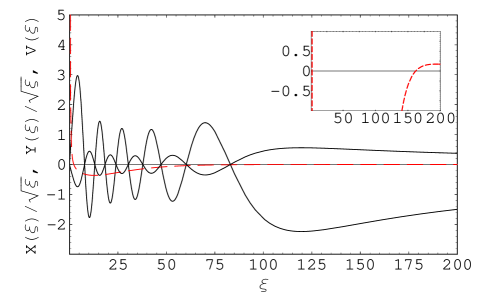
Figure 1: Soliton profile. Stokes and pump fields (black) (assumed real) and the potential (dashed red) both in arbitrary units vs $\xi={\cal M}\rho$ are shown for the refractive index $\nu=\sqrt{2}$, the field ratio at the origin $r(0)=-0.25$ (essentially fixed at all $\xi$), and $\xi_{0}=12.43\cdots$. The barrier region of the potential is expanded by $10^{4}$ in the inset.

Relation between the soliton mass ${\cal M}$ and the soliton size $\rho_{0}$ is roughly ${\cal M}\rho_{0}=O[\xi_{s}]$, with $\xi_{s}$ one of the eigenvalues. The soliton size can be anywhere between atomic distance ($\sim$ 1nm in solids) and target size, maximally the transverse size of laser irradiated region, but most likely sizes of order the wavelength of triggering laser are the main component. For numerical estimate below we assume for definiteness ${\cal M}=\xi_{s}\pi/(2\rho_{0})$, often taking $\xi_{s}=1$ for crude estimates.

One might characterize the photonic soliton by saying that it is a stable concentration of fields, possibly much below the field wavelength scale, supported by surrounding dense, excited target atoms.

Implication to radiative neutrino pair emission       We discuss neutrino pair emission $|1\rangle\rightarrow|2\rangle+\gamma+\nu_{i}\nu_{j}$, the pair emission caused by the Hamiltonian density, ${\cal H}_{W}=g_{W}j_{\nu}^{\dagger}R_{31}+({\rm h.c.})$ with $j_{\nu}^{\dagger}$ the neutrino pair emission current. Features of a single photon energy spectrum, angular distribution and distinction from two photon process have been discussed using a different approach in [8]. Here we investigate this problem using MB equations, and examine effect of soliton formation.

The transition amplitude for radiative neutrino pair emission after soliton formation is governed by the following equation written in the interaction picture,

$$\partial_{t}R_{21}=\frac{d_{2}g_{W}}{4\Delta}nj_{\nu}^{\dagger}{\cal E}_{s}\frac{1-\eta r^{2}}{1+\eta r^{2}}e^{-i({\cal M}-E_{\nu\nu}-E_{\gamma})(t\pm z)}\,,$$ (13)

where $E_{\nu\nu}(E_{\gamma})$ is the energy going into neutrinos (photons). A large soliton mass of ${\cal M}\gg\Delta$ appears in the exponential factor.

The large time limit for the transition rate per unit volume $d|R_{21}(t)|^{2}/dt$ can be worked out by using the wave function of soliton ${\cal E}_{s}(\rho)e^{im\theta}e^{\pm i({\cal M}-E_{\nu\nu}-E_{\gamma})z}$, resulting in a similar formula to the Fermi golden rule, with a difference of large energy factor ${\cal M}-E_{\nu\nu}-E_{\gamma}$. How the total rate scales with the total number of target atoms is as follows. We may take the maximal magnitude ${\cal E}_{s}$ of order ${\cal M}/d_{2}$, along with $r=0$. The enhancement factor per unit atom is $\>K=|{\cal E}_{s}/e|^{2}(V\Delta^{3}/2\pi^{2})(2\Delta/{\cal M})\sim 1/(\pi d_{2}^{2}\rho_{0}\Delta^{3})\,,\>$ where $e\sim\sqrt{\Delta/2V}\sim\Delta^{2}/\sqrt{2}$ is the field magnitude of a single atom transition, and the inverse of the last factor ${\cal M}/2\Delta$ is the number of events for the soliton decay. One has the entire enhancement factor for $N$ target atoms given by $KN^{2}$, where

$$K\sim 2.4\times 10^{8}\xi_{s}(\frac{{\rm nm}}{\rho_{0}})(\frac{{\rm eV}}{\Delta})^{3}(\frac{10^{-8}{\rm cm}}{d_{2}})^{2}\,.$$ (14)

What happens is formation of soliton of mass ${\cal M}$, which macroscopically decays. This massive soliton goes into many radiative pairs. The microscopic description of this phenomenon is that the rate of elementary radiative neutrino pair emission is enhanced by an extra factor, $O[{\cal M}/(d_{2}^{2}\Delta^{3})\sim 1/(d_{2}^{2}\rho_{0}\Delta^{3})]$ in addition to the usual coherence factor $N^{2}$.

The elementary rate $\gamma$ of radiative neutrino pair emission is roughly given by
$\>\gamma_{\gamma\nu\nu}=G_{F}^{2}\Delta_{12}^{5}(\gamma_{32}/\Delta_{32})(\Delta_{12}/\Delta_{31})^{2}/(15\pi^{5})\sim 3.3\times 10^{-34}s^{-1}(\Delta_{12}/{\rm eV})^{5}(\gamma_{32}/\Delta_{32})(\Delta_{12}/\Delta_{31})^{2}\,.\>$ For noble gas atoms implanted with a fraction $10^{-3}$ in solid para-H₂ matrix, the maximum rate is $4\times 10^{-27}s^{-1}N^{2}$ for Ar and $2\times 10^{-28}s^{-1}N^{2}$ for Xe, giving the total rate of order (40 - 2)Hz for $N=10^{14}$ (we took $\xi_{s}=1$ for this estimate). Other noble gas atoms in solid matrix give similar rates, somewhat larger for Ne by $O[400]$ than Xe. Alkaline earth and other atoms often give much smaller rates. The enhanced rate scales with $\Delta_{12}^{4}\Delta_{32}^{2}/(\Delta_{31}^{2}\rho_{0})$ of target parameters, which works to give large rates for the $\Lambda-$type noble gas atoms, with large $\Delta_{i2}$ and small $\Delta_{31}$.

The precise angular distribution of photon in radiative neutrino pair emission depends on how the triggering laser irradiation leads to formation of solitons, their number and their size distribution, which is a difficult problem to solve. But, the angular distribution from decay of a single soliton can be worked out from (13). Without much calculation we may deduce basic features of photon angular distribution by noting combined spatial variation of field and neutrino pair ${\cal E}_{s}j_{\nu}^{\dagger}$. The phase factor in the exponent, which needs to be canceled, is $\left((\pm{\cal N}+K_{\rho})\rho+(\pm\kappa+K_{z})z+(m+m_{\nu\nu})\theta\right)$, with $K_{i}$ the momenta of many neutrino pairs. The correlation to the cylinder axis is evident, and the photon emission is confined to a small angle region of $\theta\leq O[\kappa/{\cal M}=(\nu^{2}-1)n(\xi_{0})/n_{0}]$.

On the other hand, two photon process has in RHS of eq.(13) $\>d_{1}d_{2}n{\cal E}_{s}^{*}{\cal E}_{p}^{*}(1-\eta r^{2})/(4\Delta(1+\eta r^{2})\,)e^{iE_{\gamma\gamma}(t\pm z)}\,,\>$ in which the soliton mass ${\cal M}$ is missing in the exponent. Thus, two photon emission from solitons do not occur. The two photon process however can occur from amplified pump and Stokes field not related to soliton formation, to give a rate simply proportional to $N^{2}$. Thus, the rate for radiative neutrino pair emission, is more enhanced, at least by the factor $r^{-2}{\cal M}/(d_{2}^{2}\Delta^{3})\sim r^{-2}/(d_{2}^{2}\rho_{0}\Delta^{3})$, than for two photon emission, which is of order $10^{5}r^{-2}$ or more for noble gas atoms in solid matrix. Incidentally, the elementary rate for two photon emission from a single atom is estimated $O[1]{\rm sec}^{-1}$ for noble gas atoms.

Controled two photon emission, however, becomes possible by using a systematic destruction of coherence, such as abrupt modulation of dielectric constant. It should also be noted that stability, and possibility of controled coherence breaking, of PS gives an ideal mechanism of enhancing the signal to the 2 photon background ratio in measurement of forbidden processes.

The potential background of multi-photon (more than 2 photon) emission is not enhanced at all by soliton formation, thus when the elementary rate of multi-photon QED process is smaller than the enhanced rate of radiative neutrino pair emission, say $O[1]$Hz, the multi-photon emission does not become the major background.

Applications and outlook       Here we briefly discuss some possible technological applications using two photon emission caused by controled destruction of stable PS’s.

Topological solitons, both stable or unstable (the case of resonance), are likely to be created in the region of high dielectric constant $\epsilon$. One may use for preparation the photonic crystal type of medium [12] doped by target atoms of long-lived $\Lambda-$type level such as Ba D-levels. Many photonic solitons of small size may be created when an array disk made of rectangular shaped high $\epsilon$ material is irradiated by the Bessel laser beam of chirality 1 for the trigger. This might serve for the memory storage. On the other hand, when a cylinder made of many high $\epsilon$ tubes is irradiated by a Bessel beam of large aperture, one may expect creation of many PS’s of long size, which might serve for efficient light transportation. From energetic reasons we expect that PS’s of size of order the laser wavelength are more likely to be created at its formation.

Correlation of emitted two pulsed lights after controled coherence breaking is excellent, in direction, energy, and chirality. Correlated emission of strong light pulses after PS destruction may thus be useful for quantum information.

What is pressing is experimental confirmation of the basic idea in the present work, and is to clarify how easy or how difficult it is to creat many PS’s using material technologically available at present. On theoretical side calculation of dynamical time evolution is left to further work.

Acknowledgements       We should like to thank for our collaborators of SPAN group, A. Fukumi, K. Nakajima, I. Nakano, and H. Nanjo for enlightening discussions on this and related subjects.

References

• [1] R.H. Dicke, Phys. Rev.93, 99(1954).
• [2] J.C. MacGillivray and M.S. Feld, Phys. Rev.A 14, 1169(1976).
• [3] F. Haake, H. King, G. Schroeder, J. Haus, and R. Glauber, Phys. Rev.A 20, 2047(1979).
• [4] For a review of superradiance, M. Benedict, A.M. Ermolaev, V.A. Malyshev, I.V. Sokolov, and E.D. Trifonov, Super-radiance Multiatomic coherent emission, Informa (1996).
• [5] S. Inouye et al., Science285, 571 (1999).
• [6] Y. Yoshikawa et al., Phys. Rev. Lett.94, 083602(2005); Phys. Rev.A 69, 041603(R) (2004).
• [7] M. Yoshimura, Phys. Rev.D75, 113007(2007).
• [8] M. Yosimura, C.Ohae, A.Fukumi, K. Nakajima, I. Nakano, H. Nanjo, and N. Sasao, Macro-coherent two photon and radiative neutrino pair emission, arXiv 805.1970[hep-ph](2008). M. Yoshimura, Neutrino Spectroscopy using Atoms (SPAN), in Proceedings of 4th NO-VE International Workshop, edited by M. Baldo Ceolin(2008).
• [9] T. Takahashi and M. Yoshimura, Effect of Relic Neutrino on Neutrino Pair Emission from Metastable Atoms, hep-ph/0703019.
• [10] To the best of our knowledge, the terminology of photonic soliton has been used in the literature in rahter imprecise ways. Our terminology is based on the topological winding number and solutions of MB equation, and has no direct connection to the ones used in literature.
• [11] For non-zero $\Omega_{ii}>0$ there may exist, for a large $\sqrt{\nu^{2}-1}\xi_{0}$, resonance solutions in their energy vicinity. They are time dependent solutions of the form, $\psi(x\,,t)=e^{-iE_{*}t-\gamma_{*}t/2}u(x)$, where $\>\left(-d^{2}/dx^{2}+V(x)\right)u(x)=(E_{*}-i\gamma_{*}/2)u(x)\>$ with resonance parameters, real $E_{*}\,,\gamma_{*}>0$. Their presence implies instability when we consider time evolution towards soliton formation. Unstable resonances, if their lifetimes are large enough, are however useful to initiate two photon emission.
• [12] J.D. Joannopoulos et al., Photonic Crystals , 2nd edition, Princeton University Press (2008).