Stability analysis on the finite-temperature replica-symmetric and first-step replica-symmetry-broken cavity solutions of the random vertex cover problem

Abstract

The vertex-cover problem is a prototypical hard combinatorial optimization problem. It was studied in recent years by physicists using the cavity method of statistical mechanics. In this paper, the stability of the finite-temperature replica-symmetric (RS) and the first-step replica-symmetry-broken (1RSB) cavity solutions of the vertex cover problem on random regular graphs of finite vertex-degree $K$ are analyzed by population dynamics simulations. We found that (1) the lowest temperature for the RS solution to be stable, $T_{RS}(K)$, is not a monotonic function of $K$, and (2) at relatively large connectivity $K$ and temperature $T$ slightly below the dynamic transition temperature $T_{d}(K)$, the 1RSB solutions with small but non-negative complexity values are stable. Similar results are obtained on random Poissonian graphs.

I Introduction

The vertex-cover (VC) problem, which asks to find a set of vertices of a graph such that the number of vertices in this set is less than a given value and that each edge of the graph is incident to at least one of the vertices in the set, is a prototype of NP-complete problems Garey and Johnson (1979); Hartmann and Weigt (2005) with wide range of real-world applications Breitbart et al. (2001); Park and Lee (2001); Gomez-Gardenes et al. (2006). In the last ten years, the VC problem defined on the ensemble of large random graphs was extensively studied using mean-field spin glasses methods, especially the zero-temperature cavity method Weigt and Hartmann (2001); Zhou (2003); Weigt and Zhou (2006); Zhou (2005); Zhou et al. (2007). It is found that, when the average connectivity $c$ of the random graph is such that $c<e=2.71828\cdots$, the random minimal vertex-cover (MVC) problem, which corresponds to vertex-covers of the minimal size for a given random graph, can be described by the replica-symmetric (RS) cavity theory. In this parameter range, minimal vertex-covers for a given random graph can be constructed using a leaf-removal algorithm Bauer and Golinelli (2001) or by a simple message-passing warning propagation algorithm Weigt and Hartmann (2001). When $c>e$, the RS cavity theory is insufficient for the MVC problem, but the cavity theory at the level of first-step replica-symmetry-breaking (1RSB) is still able to give accurate predictions on the average size of minimal vertex-covers Zhou (2003); Weigt and Zhou (2006) and the average ground-state entropy Zhou and Zhou (2009). Following the zero-temperature 1RSB cavity theory, a survey propagation algorithm was used in Ref. Weigt and Zhou (2006) to construct minimal vertex-covers for single random graphs.

Similar as the mean-field work on the random $K$-satisfiability problem Mézard et al. (2002); Mézard and Zecchina (2002); Mézard and Parisi (2003), the zero-temperature cavity calculations of Refs. Zhou (2003); Weigt and Zhou (2006) for the VC problem considers only the energetic effect and ignores completely the entropic effect. To have a more comprehensive understanding of the random VC problem, in the present paper a finite temperature $T$ is introduced into the VC problem. The stabilities of the mean-field RS and 1RSB cavity solution for the VC problem at finite temperature are analyzed following earlier works of Refs. Krzakala and Zdeborová (2007); Montanari et al. (2008); Zdeborová and Krzakala (2007); Zdeborová (2008); Montanari and Ricci-Tersenghi (2003); Montanari et al. (2004); F. Krzakala et al. (2004). The $T\rightarrow 0$ limit of these solutions and their stability are also studied. A similar analysis was recently carried out for the random $Q$-coloring problem by Krzakala and Zdeborova Krzakala and Zdeborová (2007). The results reported in this paper suggest that the VC problem and the $Q$-coloring problem have some important differences. On random regular graphs with connectivity $K$, for the VC problem we find that the lowest temperature for the RS solution to be stable, $T_{RS}(K)$, is not a monotonic function of $K$. The same non-monotonic behavior is observed for the VC problem on random Poisson graphs. We also find that, for random regular graphs with relatively large connectivity $K$, there is a temperature range $T_{RS}(K)<T<T_{d}(K)$ in which both a stable RS solution and a stable 1RSB solution co-exist, where $T_{d}(K)$ is the dynamical transition temperature of the system. Although the VC problem is a spin-glass problem with only two-body interactions, the numerical results of this work suggest that, for random regular graphs with relatively large connectivity $K$ and temperature $T\sim T_{d}(K)$, the 1RSB cavity solutions with small but non-negative complexity values may be stable toward further steps of replica-symmetry-breaking.

The paper is organized as follows. Section II includes some definitions. In Sec. III we consider the RS solution and its stability. In Sec. IV we consider the finite temperature 1RSB solution and its type-II stability. We also compare results obtained by the finite-temperature stability analysis with those obtained using both the energetic and the entropic zero-temperature stability analysis. We conclude this work in Sec. V. Some of the technical details are included in the two appendices of this paper.

II Definitions

Two ensembles of random graphs are considered in this paper, namely Erdös-Renyi (ER) random graphs Bollobas (2001) and regular random graphs.

An ER random graph ${\cal G}$ has $N$ vertices and $M=(c/2)N$ different edges, where the edges are chosen completely random from the set of $N(N-1)/2$ candidate edges between vertex-pairs. An edge of the graph which links between vertices $i$ and $j$ is denoted by $(i,j)$. The vertex degree $k_{i}$ of a vertex $i$ is equal to the number of edges that are linked to vertex $i$. The mean value of vertex degrees as averaged over all the vertices of graph ${\cal G}$ is equal to $c$. For a large ER random graph, the fraction of vertices with a given degree $k$ is given by the Poisson distribution $f_{c}(k)\equiv e^{-c}c^{k}/k!$. Because of this reason, an ER random graph is also called a Poisson random graph.

A regular random graph has $N$ vertices and $M=(K/2)N$ edges, with each vertex having exactly $K$ edges. The $M$ edges in a regular random graph are randomly connected under the constraint that each vertex has $K$ edges attached.

A vertex cover of graph ${\cal G}$ is a subset of vertices $U$ that covers all edges. Here, cover means that for each edge $(i,j)$ in the graph at least one of the two end vertices is in the set $U$. We denote the state of each vertex $i$ by a Ising spin $\sigma_{i}\in\{\pm 1\}$: $\sigma_{i}=-1$ if $i\in U$ and $\sigma_{i}=+1$ if otherwise. All the vertex covers of graph ${\cal G}$ form a solution sub-space out of the total number of $2^{N}$ possible spin configurations. Each vertex cover $\{\sigma_{i}\}\equiv\{\sigma_{1},\sigma_{2},\ldots,\sigma_{N}\}$ is assigned an energy

$$E\left(\{\sigma_{i}\}\right)=\sum_{i=1}^{N}\delta_{\sigma_{i},-1}$$ (1)

which is equal to the cardinality of the vertex cover.

We introduce a temperature $T$ and weight each vertex cover by the Boltzmann factor $e^{-\beta E}$, where $\beta=1/T$ is called the inverse temperature. The total partition function $Z$ and the free energy $F(\beta)$ are then defined by

$$Z\equiv e^{-\beta F(\beta)}=\sum_{\left\{\sigma_{i}\right\}}e^{-\beta E\left(\left\{\sigma_{i}\right\}\right)}\prod_{(i,j)}\bigl{(}1-\delta_{\sigma_{i},1}\delta_{\sigma_{j},1}\bigr{)}\ ,$$ (2)

and the Gibbs measure for each vertex cover is

$$\mathcal{P}\left(\{\sigma_{i}\}\right)=\frac{1}{Z}e^{-\beta E\left(\{\sigma_{i}\}\right)}\prod_{(i,j)}\bigl{(}1-\delta_{\sigma_{i},1}\delta_{\sigma_{j},1}\bigr{)}\ .$$ (3)

In Eqs. (2) and (3), the term $\prod_{(i,j)}(1-\delta_{\sigma_{i},1}\delta_{\sigma_{j},1})$ is equal to unity or zero depending on whether the spin configuration corresponds to a vertex-cover or not. Only vertex-covers contribute to the free-energy of the system. The $T\rightarrow 0$ limit of Eq. (2) corresponds to the MVC problem. In this case, only those ground-state solutions have non-zero Gibbs measure.

Under the Gibbs measure Eq. (3) the marginal probability $\pi_{i}$ of a vertex $i$ being covered is expressed as

$$\pi_{i}=\sum_{\{\sigma_{j}\}}\mathcal{P}\left(\{\sigma_{j}\}\right)\delta_{\sigma_{i},-1}\ .$$ (4)

$\pi_{i}$ is called the cover ratio of vertex $i$. A direct computation of the cover ratios $\pi_{i}$ is difficult for large random graphs, but approximate values for $\pi_{i}$ can be obtained using the cavity method.

III Stability of the Replica Symmetric Cavity Theory

III.1 The replica-symmetric cavity equations at finite temperatures

According to the replica-symmetric cavity theory Mézard and Parisi (2001), the free energy at inverse temperature $\beta$ can be calculated by

$$F(\beta)=\sum_{i\in{\cal G}}\Delta F_{i}-\sum_{(i,j)\in{\cal G}}\Delta F_{(i,j)}\ ,$$ (5)

where $\Delta F_{i}$ and $\Delta F_{(i,j)}$ are, respectively, the free energy shift due to the addition of vertex $i$ and edge $(i,j)$. The free energy expression Eq. (5) corresponds to the zeroth-order term of a loop series expansion for the total partition function Eq. (2) Chertkov and Chernyak (2006). The set of nearest-neighbors for a vertex $i$ is denoted as $\partial i$. Because of the locally tree-like structure of a random graph ${\cal G}$, in the absence of vertex $i$, the length of the shortest paths between two vertices $j,k$ in the set $\partial i$ diverges logarithmically with the graph size $N$. It is then assumed that in the absence of vertex $i$ the spin values on the vertices of the set $\partial i$ are mutually independent. Under this Bethe-Peierls approximation, the free energy shift associated with the addition of vertex $i$ is expressed as

$$\Delta F_{i}=-\frac{1}{\beta}\log\Bigl{(}e^{-\beta}+\prod_{j\in\partial i}\pi_{j|i}(\beta)\Bigr{)}\ ,$$ (6)

where $\pi_{j|i}(\beta)$ is the probability of vertex $j$ being covered in the absence of vertex $i$. In Eq. (6), the term $e^{-\beta}$ corresponds to vertex $i$ being covered ($\sigma_{i}=-1$), while the term $\prod_{j\in\partial i}\pi_{j|i}$ corresponds to vertex $i$ being uncovered (then all the neighbors of $i$ need to be covered). Under the same Bethe-Peierls approximation, the free energy shift $\Delta F_{(i,j)}$ is expressed as

$$\Delta F_{(i,j)}=-\frac{1}{\beta}\log\Bigl{(}1-\bigl{(}1-\pi_{i|j}(\beta)\bigr{)}(1-\pi_{j|i}(\beta)\bigr{)}\Bigr{)}\ .$$ (7)

The free energy $F$ as expressed by Eq. (5) is a functional of the $2M$ cavity probabilities $\{\pi_{j|i}\}$, two on each edge $(i,j)$. At equilibrium, the free energy $F$ should reach a minimal value. Then the variational condition

$$\frac{\delta F}{\delta\pi_{j|i}}=0$$ (8)

leads to the following iterative equation for each cavity probability $\pi_{j|i}$:

$$\pi_{j|i}=\mathcal{F}_{RS}\left(\left\{\pi_{k|j}\right\}\right)=\frac{e^{-\beta}}{e^{-\beta}+\prod_{k\in\partial j\backslash i}\pi_{k|j}(\beta)}\ ,$$ (9)

where $\partial j\backslash i$ denotes the remaining set after vertex $i$ is removed from set $\partial j$. When a fixed point is reached for the set of iterative equations Eq. (9), the mean energy $\langle E\rangle$ and entropy $S$ of the system are then calculated according to

$$\langle E\rangle = \frac{{\rm d}\beta F}{{\rm d}\beta}=\sum_{i}\frac{e^{-\beta}}{e^{-\beta}+\prod\limits_{j\in\partial i}\pi_{j|i}(\beta)}\ ,$$ (10)

$$S = \beta\bigl{(}\langle E\rangle-F\bigr{)}\ .$$ (11)

For a single graph ${\cal G}$, we denote by $\mathcal{P}_{RS}(\pi)$ the probability of observing a cavity probability with value $\pi_{j|i}=\pi$, namely

$$\mathcal{P}_{RS}(\pi)=\frac{1}{2M}\sum\limits_{(i,j)\in{\cal G}}\Bigl{(}\delta\bigl{(}\pi_{j|i}(\beta)-\pi\bigr{)}+\delta\bigl{(}\pi_{i|j}(\beta)-\pi\bigr{)}\Bigr{)}\ ,$$ (12)

where $\delta(x)$ is the Dirac delta function. When the size $N$ of a random graph ${\cal G}$ is sufficiently large, the probability distribution $P(\pi)$ becomes independent of the detailed connection pattern of the graph. It only depends on the vertex degree profile of the graph and the inverse temperature $\beta$. We can write down the following self-consistent equation for $P(\pi)$:

$$\mathcal{P}_{RS}(\pi)=p_{nn}(1)\delta\Bigl{(}\pi-\frac{e^{-\beta}}{e^{-\beta}+1}\Bigr{)}+\sum\limits_{k=1}^{\infty}p_{nn}(k+1)\int\prod_{j=1}^{k}\Bigl{[}{\rm d}\pi_{j}\mathcal{P}_{RS}(\pi_{j})\Bigr{]}\delta\Biggl{(}\pi-\frac{e^{-\beta}}{e^{-\beta}+\prod_{j=1}^{k}\pi_{j}}\Biggr{)}\ .$$ (13)

In Eq. (13), $p_{nn}(k+1)$ is the probability that a randomly chosen nearest-neighbor of a vertex have vertex degree $k+1$.

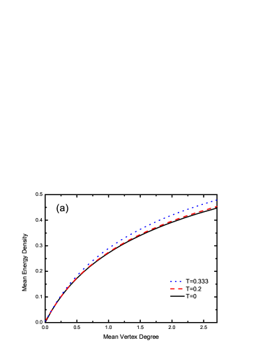
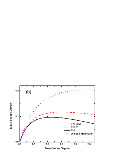
Figure 1: (Color Online) Mean vertex-cover energy density and entropy density as a function of the mean vertex degree of the ER random graph. Different curves correspond to different temperature $T$. The circular symbols are simulation results of Ref. Weigt and Hartmann (2001).

For ER random graphs, $p_{nn}(k+1)=(k+1)f_{c}(k)/c=f_{c}(k)$, i.e., it is also a Poisson distribution. A fixed-point solution for Eq. (13) can be obtained by population dynamics simulation Mézard and Parisi (2001). In terms of the cavity probability distribution $\mathcal{P}_{RS}(\pi)$, the densities for the free energy, mean energy, and entropy can be re-written as

$$f\equiv F/N = -\frac{1}{\beta}f_{c}(0)\log\bigl{(}e^{-\beta}+1\bigr{)}-\frac{1}{\beta}\sum_{k=1}^{\infty}f_{c}(k)\int\prod_{j=1}^{k}\Bigl{[}{\rm d}\pi_{j}\mathcal{P}_{RS}(\pi_{j})\Bigr{]}\log\Bigl{(}e^{-\beta}+\prod_{j=1}^{k}\pi_{j}\Bigr{)}$$ (14)

$$+\frac{c}{2\beta}\int{\rm d}\pi_{i}\mathcal{P}_{RS}(\pi_{i}){\rm d}\pi_{j}\mathcal{P}_{RS}(\pi_{j})\log\bigl{(}1-(1-\pi_{i})(1-\pi_{j})\bigr{)}\ ,$$

$$\bar{e}\equiv\langle E\rangle/N = f_{c}(0)\frac{e^{-\beta}}{e^{-\beta}+1}+\sum\limits_{k=1}^{\infty}f_{c}(k)\int\prod\limits_{j=1}^{k}\Bigr{[}{\rm d}\pi_{j}\mathcal{P}_{RS}(\pi_{j})\Bigr{]}\frac{e^{-\beta}}{e^{-\beta}+\prod_{j=1}^{k}\pi_{j}}\ ,$$ (15)

$$s\equiv S/N = \beta(\bar{e}-f)\ .$$ (16)

The mean energy and entropy density of the vertex-cover problem on ER random graphs of mean degree $c<2.7183$ are shown in Fig. 1. At a given value of $\beta$, the mean energy density increases continuously with the mean vertex degree $c$. On the other hand, the mean entropy first increases with $c$ when $c$ is small and then decreases with $c$ when $c$ exceeds certain temperature-dependent value.

For regular random graphs, $p_{nn}(k+1)$ in Eq. (13) is expressed as $p_{nn}(k+1)=\delta_{k}^{K-1}$. In the replica-symmetric cavity theory, it is therefore assumed that the cavity cover ratio distribution $\mathcal{P}_{RS}(\pi)$ is a Dirac delta function $\mathcal{P}_{RS}(\pi)=\delta(\pi-\pi_{*})$, with $\pi_{*}$ determined by

$$\pi_{*}e^{-\beta}+\pi_{*}^{K}-e^{-\beta}=0\ .$$ (17)

The mean free energy density and energy density are calculated by

$$f = -\frac{1}{\beta}\log(e^{-\beta}+\pi_{*}^{K})+\frac{K}{2\beta}\log(2\pi_{*}-\pi_{*}^{2})\ ,$$ (18)

$$\bar{e} = \frac{e^{-\beta}}{e^{-\beta}+\pi_{*}^{K}}\ .$$ (19)

III.2 The entropic zero-temperature limit

The energetic zero-temperature limit of the RS cavity theory is very easy to implement. In this limit, one only interests in whether a given vertex is always uncovered among all the MVCs, and a warning propagation algorithm can be constructed for the vertex-cover problem in this limit Weigt and Zhou (2006). In this subsection, we study the entropic zero-temperature limit so that the entropy of MVCs can also be calculated.

It is helpful to define two auxiliary parameters $\eta_{i}(\beta)$ and $\eta_{j|i}(\beta)$ through

$$\eta_{i}(\beta) = \frac{1}{\beta}\log\Bigl{(}\frac{\pi_{i}(\beta)}{1-\pi_{i}(\beta)}\Bigr{)}\ ,$$ (20)

$$\eta_{j|i}(\beta) = \frac{1}{\beta}\log\Bigl{(}\frac{\pi_{j|i}(\beta)}{1-\pi_{j|i}(\beta)}\Bigr{)}\ .$$ (21)

The physical meanings of $\eta_{i}$ and $\eta_{j|i}$ are obvious: $\beta\eta_{i}=\log[\pi_{i}/(1-\pi_{i}]$ is the log-likelihood of vertex $i$ being covered, and $\beta\eta_{j|i}$ is the log-likelihood of vertex $j$ being covered in the absence of vertex $i$. The iterative equation (9) can be rewritten as

$$\eta_{j|i}(\beta)=-1+\sum\limits_{k\in\partial j\backslash i}\frac{1}{\beta}\log\bigl{(}1+e^{-\beta\eta_{k|j}}\bigr{)}\ .$$ (22)

At $T\rightarrow 0$ ($\beta\rightarrow+\infty$) we assume that

$$\eta_{j|i}=m_{j|i}+\frac{r_{j|i}}{\beta}\ ,$$ (23)

with $m_{j|i}$ being an integer and $r_{j|i}$ being a finite real value. Then From Eq. (22) we get the iteration equations for $m_{j|i}$ and $r_{j|i}$:

$$m_{j|i} = -1+\sum\limits_{k\in\partial j\backslash i}\Theta(-m_{k|j})\ ,$$ (24)

$$r_{j|i} = \sum\limits_{k\in\partial j\backslash i}\Bigl{[}\bigl{(}1-\Theta(|m_{k|j}|)\bigr{)}\log(1+e^{-r_{k|j}})-\Theta(-m_{k|j})r_{k|j}\Bigr{]}\ ,$$ (25)

where $\Theta(x)$ is the Heaviside function defined by $\Theta(x)=1$ for $x>0$ and $\Theta(x)=0$ for $x\leq 0$.

At the limit of $\beta\rightarrow\infty$, the free energy Eq. (14), energy Eq. (15), and entropy Eq. (16) can all be expressed in terms of $\{m_{j|i},r_{j|i}\}$. From these expressions, the mean ground-state energy and entropy densities of the VC problem on an ER random graph can easily be evaluated by population dynamics. The theoretical predictions on the mean energy and entropy density of the MVC problem are also shown in Fig. 1, together with the simulation results of Weigt and Hartmann Weigt and Hartmann (2001). For mean connectivity $c<2.7183$ the agreement between theory and simulation results is good. In the population dynamics simulation, we have noticed that when $c>2.7183$, the amplitude of some $r_{j|i}$ values approaches infinity when $m_{j|i}=0$. Such type of divergence then lead to a negative value for the entropy density of the MVC problem (see also Ref. Zhou and Zhou (2009)). As we will discuss in the next subsection, for ER random graphs with $c>2.7183$, the zero-temperature RS cavity theory is no longer valid and a more advanced mean-field theory is needed.

We notice that, the divergence of the residue fields $r_{j|i}$ as observed for the random MVC problem does not occur in the random maximal matching problem Zdeborová and Mézard (2006). For the random maximal matching problem, the RS cavity theory is stable at any temperature.

III.3 Stability of the replica-symmetric solution

At low enough temperatures and/or high mean vertex degrees, the Bethe-Peierls approximation used in the RS cavity equations is no longer valid. Then the RS cavity theory becomes unstable to higher levels of replica-symmetry-breaking. The stability of the RS cavity equations can be checked by studying the point-to-set correlations in the graph Krzakala et al. (2007); Mézard and Montanari (2006); Montanari and Semerjian (2006). If these correlations do not decay to zero at large distances, then non-trivial solutions exist for the one-step replica-symmetry-breaking (1RSB) cavity equations at Parisi parameter $m=1$. The dynamical transition temperature $T_{d}$, which is defined by the critical temperature where point-to-set correlation begin to diverge, can be checked using 1RSB equations at $m=1$(see Appendix A for a detailed calculation of $T_{d}$).

A easier way to check the validity of the RS assumption is to study the local stability of the RS solution. This local stability analysis leads to a threshold temperature $T_{RS}$. However, the local stability of the RS solution is a necessary but not a sufficient condition for RS correctness and in general, $T_{RS}\leq T_{d}$. In this paper, the way of checking the local stability of the RS solution is to study the spin-glass susceptibility Zdeborová (2008); Zdeborová and Mézard (2006) as defined by

$$\chi_{SG}=\frac{1}{N}\sum_{i\neq j}\langle\sigma_{i}\sigma_{j}\rangle_{c}^{2}\ ,$$ (26)

where $\langle\sigma_{i}\sigma_{j}\rangle_{c}\equiv\langle\sigma_{i}\sigma_{j}\rangle-\langle\sigma_{i}\rangle\langle\sigma_{j}\rangle$ is the connected correlation between vertex $i$ and vertex $j$. The above equation can be re-expressed as

$$\chi_{SG}=\frac{2}{N}\Bigl{[}N_{1}\overline{\langle\sigma_{i}\sigma_{j(1)}\rangle_{c}^{2}}+N_{2}\overline{\langle\sigma_{i}\sigma_{j(2)}\rangle_{c}^{2}}+\ldots+N_{d}\overline{\langle\sigma_{i}\sigma_{j(d)}\rangle_{c}^{2}}+\ldots\Bigr{]}\ ,$$ (27)

where $N_{d}$ is the total number of vertex-pairs of distance (minimum path length) $d$ in the graph ${\cal G}$; $\sigma_{j(d)}$ denotes a vertex $j$ which is separated from vertex $i$ by a distance $d$; and $\overline{\langle\sigma_{i}\sigma_{j(d)}\rangle_{c}^{2}}$ denotes the mean value of $\langle\sigma_{i}\sigma_{j(d)}\rangle_{c}^{2}$ as averaged over all the $N_{d}$ vertex-pairs $(i,j)$ of distance $d$. For a large ER random graph with mean connectivity $c$, $N_{d}=N(c^{d}/2)$ when $d$ is much smaller than the length of a typical loop in the graph ($d<\log_{c}N$), while for a large regular random graph with vertex degree $K$, the scaling is $N_{d}=NK(K-1)^{d-1}/2$. On the other hand, using the locally tree-like property of a random graph $\mathcal{G}$, it can be shown that

$$\overline{\langle\sigma_{i}\sigma_{j(d)}\rangle_{c}^{2}}\propto\lambda^{(d-1)}\ ,$$ (28)

where

$$\lambda(\beta)=\overline{\Biggl{[}\frac{\partial\pi_{j|i}}{\partial\pi_{k|j}}\Biggr{]}^{2}}=\overline{\Biggl{[}\frac{e^{-\beta}\prod_{l\in\partial j\backslash i,k}\pi_{l|j}(\beta)}{\bigl{(}e^{-\beta}+\prod_{l\in\partial j\backslash i}\pi_{l|j}(\beta)\bigr{)}^{2}}\Biggr{]}^{2}}\ .$$ (29)

In the above equation, the overline means averaging over all the paths $k\rightarrow j\rightarrow i$ of length two in the graph $\mathcal{G}$.

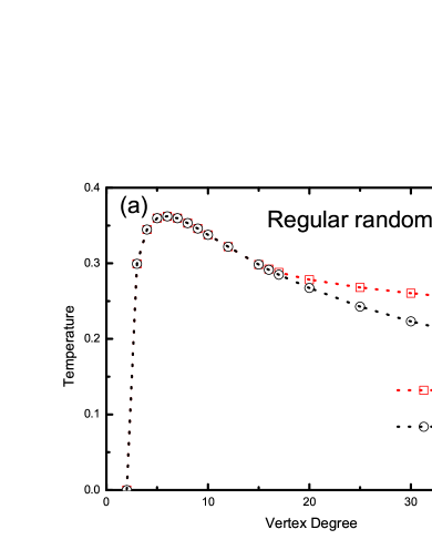
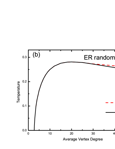
Figure 2: (a) RS local instability temperature $T_{RS}$ and dynamical transition temperature $T_{d}$ of the vertex-cover problem on regular random graphs (a) and ER random graphs (b). When $T<T_{RS}$, RS solution become locally unstable; When $T<T_{d}$, 1RSB solution at $m=1$ has non-trivial solution.

For a regular random graph, the spin-glass susceptibility $\chi_{SG}$ remains finite in the thermodynamic limit of $N\rightarrow\infty$ if and only if $(K-1)\lambda(\beta)<1$. This condition is re-expressed as

$$(K-1)\Biggl{[}\frac{e^{-\beta}\pi_{*}^{K-2}}{\left(e^{-\beta}+\pi_{*}^{K-1}\right)^{2}}\Biggr{]}^{2}<1\ ,$$ (30)

where $\pi_{*}$ is the solution of Eq.(17).

The local stability boundary for the RS cavity theory as predicted by Eq. (30) and the dynamical transition temperature $T_{d}$ are shown in Fig. 2a. At $K=2$, the RS solution is locally stable at any temperature. When $K\geq 3$ the RS solution is only stable at temperatures $T>T_{RS}$. The critical temperature $T_{RS}$ is not a monotonic function of graph degree $K$ but rather has a maximal value at $K=6$. Such a re-entrant behavior is also observed for random ER graphs (Fig. 2b). It is not yet clear why the RS solution of the VC problem on a random regular graph of $K=6$ is the most easiest to be unstable. At small values of $K$, $T_{d}=T_{RS}$ . But when $K\geq 16$, $T_{d}>T_{RS}$. The 1RSB solution at $m=1$ (see the next section and Appendix A) begins to have a non-trivial solution at $T=T_{d}$, suggesting that the configuration space of the system starts to splitting into many Gibbs pure states. In the temperature region $T_{RS}<T<T_{d}$, although the RS solution still remains locally stable, it does not correctly describe the property of the system. In our numerical solutions, we find that the Kauzmann temperature $T_{K}$, which corresponds to zero complexity ($\Sigma\left(m=1\right)=0$, see next section), is always equal to $T_{d}$.

For an ER random graphs, the convergence condition for the spin-glass susceptibility $\chi_{SG}$ is $c\lambda(\beta)<1$. For this ensemble of graphs, we can not determine the stability boundary analytically. Instead, we iterate a stability parameter $\Delta_{i|f}$ in population using population dynamics, where

$$\Delta_{i|f}=\sum_{j\in\partial i\backslash f}\left[\frac{e^{-\beta\prod_{j^{\prime}\neq j}\pi_{j^{\prime}|i}}}{\left(e^{-\beta}+\prod_{j\in\partial i\backslash f}\pi_{j|i}^{2}\right)}\right]^{2}\Delta_{j|i}.$$ (31)

If $\Delta_{j|f}<1$ after iterating for a long enough time, the RS solution is then locally stable; otherwise it is locally unstable. The local stability boundary for the RS cavity solution is shown in Fig. 2b. When $c<2.7183$ the RS solution is always stable and 1RSB equation at $m=1$ has trivial solution. When $c>e$, the RS solution is stable at high temperatures and becomes unstable blow a threshold temperature $T_{RS}(c)$. The threshold temperature $T_{RS}(c)$ has a maximal value at mean vertex-degree $c\approx 20$. Similar with those of regular random graphs, $T_{d}=T_{RS}$ at relative small average connectivity and $T_{d}$ becomes larger than $T_{RS}$ when $c>=30$.

III.4 Infinite-connectivity limit

When the connectivity ($c$ for ER graphs and $K$ for regular random graphs) is large, we see from Eq. (9) that $\pi_{j|i}$ should be very close to $1$. In the case of regular random graphs, the solution at the $K\to\infty$ limit of Eq. (17) has the following property

$$\lim_{K\to\infty}\pi_{\star}^{K}=0\ ,\;\;\;\lim_{K\to\infty}\pi_{\star}=1\ .$$ (32)

At this limit, the free energy density and mean energy density both equal to unity, and the entropy density is zero. This means that when the connectivity goes to infinity, there is only one vertex cover for the graph which includes all the vertices. At $K\rightarrow\infty$, the local stability condition for the RS solution is

$$\lim_{K\to\infty}\pi_{\star}^{2K-4}\left(K-1\right)e^{2\beta}<1\ ,$$ (33)

which is satisfied at any finite temperature. Therefore the RS solution is locally stable at any finite temperature for an infinitely connected regular random graph.

For ER random graphs, we do not have an analytical expression for the large $c$ limit, but we have checked by population dynamics simulations that the results are the same as those in regular random graphs: the cover ratio and the energy density both go to unity, the entropy density goes to zero and the RS solution is locally stable at any finite temperature.

IV Stability of the first-step replica-symmetry-broken cavity solution

IV.1 1RSB solution at finite temperatures

When the RS mean-field solution to the random vertex-cover problem is unstable, one can try to describe the system using the first-step replica-symmetry-breaking (1RSB) spin-glass theory. In the 1RSB theory, the configuration space of the system is divided into many sub-spaces or macrostates. Each macrostate $\alpha$ has a free energy $F_{\alpha}(\beta)$ and its contribution to the statistical property of the system is weighted by a Boltzmann factor $\exp\bigl{(}-yF_{\alpha}(\beta)\bigr{)}$, where $y$ is the adjustable inverse temperature at the level of macrostates. The ratio $m\equiv y/\beta=yT$ is called the Parisi parameter. The grand free energy density (also called the replicated free energy density) $g(y,\beta)$ is defined as

$$g(y,\beta)=-\frac{1}{Ny}\log\Bigl{(}\sum\limits_{\alpha}\exp\bigl{(}-yF_{\alpha}(\beta)\bigr{)}\Bigr{)}=-\frac{1}{Ny}\log\Bigl{(}\int{\rm d}fe^{-Nyf+N\Sigma(f)}\Bigr{)}\ ,$$ (34)

where $f$ denotes the free energy density of a macrostate and $\exp(N\Sigma(f))$ is the density of macrostates with free energy density $f$. The quantity $\Sigma(f)$ is called the complexity. Taking the $N\to\infty$ limit, at saddle-point we have

$$g(y,\beta)=\min\limits_{f}\bigl{[}f-\Sigma(f)/y\bigr{]}\ .$$ (35)

The macrostates with the lowest free energy density $f_{0}(\beta)$ corresponds to the point of zero complexity, $\Sigma\bigl{(}f_{0}(\beta)\bigr{)}=0$. Depending on the value of the parameter $y$ (or equivalent the Parisi parameter $m$) the free energy density $f$ of the macrostates which contribute to the grand free energy density $g(y,\beta)$ is determined by

$$\frac{{\rm d}\Sigma(f)}{{\rm d}f}=y\ .$$ (36)

In the 1RSB cavity theory, the order parameter is no longer the cover ratio $\pi_{j|i}$ but the distribution profile $Q_{j|i}(\pi_{j|i})$ of $\pi_{j|i}$ over all the macrostates. Equation (9) is generalized into

$$Q_{j|i}(\pi_{j|i})=\mathcal{F}_{1RSB}(\{Q_{k|j}\})=\frac{1}{Z_{j|i}}\Bigl{[}\int\prod_{k\in\partial j\backslash i}{\rm d}\pi_{k|j}Q_{k|j}(\pi_{k|j})\Bigr{]}e^{-y\Delta F_{j|i}}\delta\Bigl{(}\pi_{j|i}-\frac{e^{-\beta}}{e^{-\beta}+\prod_{k\in\partial j\backslash i}\pi_{k|j}}\Bigr{)}\ ,$$ (37)

where $Z_{j|i}$ is a normalization factor, and the expression for $\Delta F_{j|i}$ is

$$\Delta F_{j|i}=-\frac{1}{\beta}\log\bigl{(}e^{-\beta}+\prod\limits_{k\in\partial j\backslash i}\pi_{k|j}(\beta)\bigr{)}\ .$$ (38)

At given inverse temperatures $\beta$ and $y$, a fixed-point solution $\{Q_{j|i}(\pi_{j|i})\}$ of Eq. (37) for a given random graph can be obtained by population dynamics. The corresponding grand free energy density $g$, mean free-energy density $\langle f\rangle$ (averaged over all the macrostates), and complexity can be obtained by the following equations:

$$g = \frac{1}{N}\sum\limits_{i}\Delta G_{i}-\frac{1}{N}\sum\limits_{(i,j)}\Delta G_{ij}\ ,$$ (39)

$$\langle f\rangle = \frac{1}{N}\sum\limits_{i}\langle\Delta F_{i}\rangle-\frac{1}{N}\sum\limits_{(i,j)}\langle\Delta F_{ij}\rangle\ ,$$ (40)

$$\Sigma = y(\langle f\rangle-g)\ .$$ (41)

In the above equations, $\Delta G_{i}$ and $\Delta G_{ij}$ are, respectively, the shift of the grand free energy of the system due to the addition of a vertex $i$ and an edge $(i,j)$:

$$\Delta G_{i} = -\frac{1}{y}\log\Bigl{[}\int\prod_{j\in\partial i}{\rm d}\pi_{j|i}Q_{j|i}(\pi_{j|i})e^{-y\Delta F_{i}}\Bigr{]}\ ,$$ (42)

$$\Delta G_{ij} = -\frac{1}{y}\log\Bigl{[}\int{\rm d}\pi_{j|i}{\rm d}\pi_{i|j}Q_{j|i}(\pi_{j|i})Q_{i|j}(\pi_{i|j})e^{-y\Delta F_{ij}}\Bigr{]}\ ;$$ (43)

and $\langle\Delta F_{i}\rangle$ and $\langle\Delta F_{ij}\rangle$ are, respectively, the mean value of the changes $\Delta F_{i}$ and $\Delta F_{ij}$ over all the macrostates:

$$\langle\Delta F_{i}\rangle = \frac{\int\prod_{j\in\partial i}{\rm d}\pi_{j|i}Q_{j|i}(\pi_{j|i})\Delta F_{i}e^{-y\Delta F_{i}}}{\int\prod_{j\in\partial i}{\rm d}\pi_{j|i}Q_{j|i}(\pi_{j|i})e^{-y\Delta F_{i}}}\ ,$$ (44)

$$\langle\Delta F_{ij}\rangle = \frac{\int{\rm d}\pi_{j|i}{\rm d}\pi_{i|j}Q_{j|i}(\pi_{j|i})Q_{i|j}(\pi_{i|j})\Delta F_{ij}e^{-y\Delta F_{ij}}}{\int{\rm d}\pi_{j|i}{\rm d}\pi_{i|j}Q_{j|i}(\pi_{j|i})Q_{i|j}(\pi_{i|j})e^{-y\Delta F_{ij}}}\ .$$ (45)

To characterize the statistical property of the vertex-cover problem on a random graph, what we need is a distribution of the distribution $Q_{j|i}(\pi_{j|i})$ among all the directed edges $j\rightarrow i$ of the graph. Let us denote this distribution as $\mathcal{P}_{1RSB}[Q(\pi)]$. Similar to Eq. (13) we can write down the following self-consistent equation for $\mathcal{P}_{1RSB}[Q]$:

$$\mathcal{P}_{1RSB}[Q(\pi)]=p_{nn}(1)\delta\Bigl{(}Q(\pi)-\delta(\pi-\frac{e^{-\beta}}{e^{-\beta}+1})\Bigr{)}+\sum\limits_{k=1}^{\infty}p_{nn}(k+1)\int\prod_{j=1}^{k}\Bigl{[}{\rm D}Q_{j}\mathcal{P}_{1RSB}(Q_{j})\Bigr{]}\delta\Biggl{(}Q(\pi)-\mathcal{F}_{1RSB}(\{Q_{j}\})\Biggr{)}\ .$$ (46)

For graphs with a general vertex degree distribution, Eq. (46) can be solved numerically by population dynamics on a two-dimensional array (see, e.g., Ref. Zhou (2008)). In the special case of random regular graphs, the probability distribution $\mathcal{P}_{1RSB}[Q]$ has a simple form: $\mathcal{P}_{1RSB}[Q(\pi)]=\delta\left(Q(\pi)-Q_{c}\left(\pi\right)\right)$. Then Eq. (46) can be re-written as a self-consistent equation for a single probability function $Q_{c}(\pi)$, and the numerical task is much simplified.

IV.2 1RSB Stability analysis

The stability of the 1RSB cavity solution is analyzed in the solution space of the second-step replica-symmetry-breaking (2RSB) cavity theory. In the 2RSB cavity theory, for each directed edge $j\rightarrow i$ the order parameter is the distribution of $Q_{j|i}(\pi_{j|i})$ over all the domains of macrostates, which is denoted by $\mathbb{Q}_{j|i}[Q]$. The iteration equation for this distribution reads

$$\mathbb{Q}_{j|i}[Q]=\frac{1}{\mathcal{Z}_{j|i}}\int\prod_{k\in\partial j\backslash i}DQ_{k|j}\mathbb{Q}_{k|j}[Q_{k|j}]e^{-y_{2}\Delta G_{j|i}}\delta\Bigl{(}Q-\mathcal{F}_{1RSB}(\{Q_{k|j}\})\Bigr{)}\,$$ (47)

where $\mathcal{Z}_{j|i}$ is a normalization constant, $y_{2}$ is the inverse temperature at the level of domains of macrostates, and $\Delta G_{k|j}$ is expressed as

$$\Delta G_{k|j}=-\frac{1}{y}\log\Bigl{[}\int\prod_{k\in\partial j\backslash i}{\rm d}\pi_{k|j}Q_{k|j}(\pi_{k|j})e^{-y\Delta F_{k|j}}\Bigr{]}\ .$$ (48)

If on each directed edge $j\rightarrow i$ the iteration equation Eq. (47) converges to the fixed-point solution $\mathbb{Q}_{j|i}[Q(\pi)]=\delta\bigl{(}Q(\pi)-Q_{j|i}(\pi)\bigr{)}$, then the 1RSB solution is said to be stable toward further steps of replica-symmetry-breaking.

According to Refs. Montanari and Ricci-Tersenghi (2003); Montanari et al. (2004); Rivoire et al. (2004), there are two types of instabilities the 1RSB cavity solution Eq. (37) can show toward non-trivial 2RSB solutions. The first type of instability (type-I instability) is state aggregation: the 1RSB macrostates aggregate into 2RSB domains, while they themselves as described by Eq. (37) contain no further internal structures. The type-I instability can be studied by tracing the propagation of a small perturbations to the distribution $Q\left(\pi_{j|i}\right)$ during the 1RSB iteration. But in practice it is rather difficult to implement such a check since the distribution $Q_{j|i}(\pi)$ has to be represented by an array in the numerical population dynamics simulation. In this paper, the type-I instability analysis is performed only at zero temperature for the energetic cavity solution but not at finite temperatures.

The second type (type-II) instability is state fragmentation: a 1RSB macrostate is itself composed of many sub-macrostates. Numerically, this type of instability can be studied by tracing the propagation of a small perturbation to $\pi_{i|j}$ during the 1RSB iteration. The easiest way to do this is the deviation of two replicas method Pagnani et al. (2003); Zdeborová (2008). One first iterates the 1RSB population dynamics to reach a steady state, and then creates a replica of the whole population and gives a small perturbation to each $\pi_{i|j}$ value of the origin population. These two populations are then updated using the same sequence of random numbers for a sufficiently long time. If the difference between the two populations decays to zero with time, then the 1RSB cavity solution is type-II stable. Another method of checking type-II stability is noise propagation: we binds a noise $\chi_{j|i}$ to each $\pi_{j|i}$ in the population. Then we iterate the population using Eq. (37) until a steady state is reached. At the same time, the values of $\chi_{j|i}$’s are updated using Eq. (31). If $\sum_{j}\chi_{j|i}$ is decreasing with iteration (equivalently, $\sum_{j}\chi_{j|i}<1$ finally), then the 1RSB iteration is stable. We have checked both methods and find that they always give the same result.

IV.2.1 The case of random regular graphs

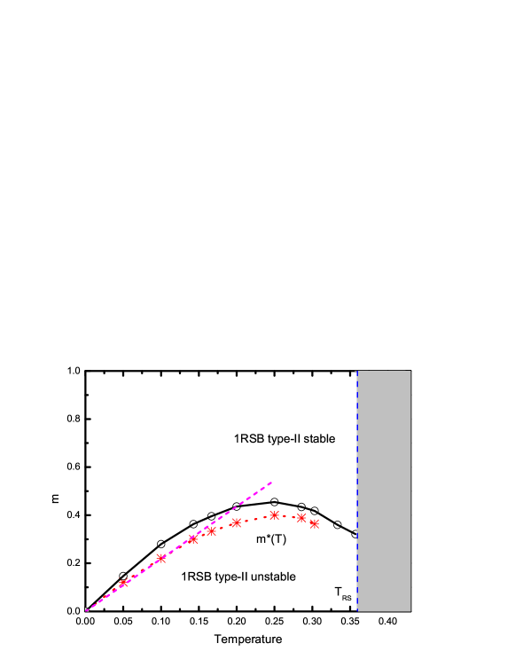
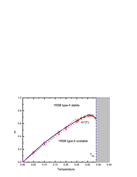
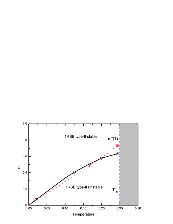
Figure 3 shows the phase diagram for the random regular graph VC problem with connectivity $K=5$. When temperature $T>T_{RS}(K=5)=0.358$ the RS solution is stable. When $T<T_{RS}(5)$ the RS solution becomes unstable and $T_{d}=T_{K}=T_{RS}$. The 1RSB solution is type-II stable only when the Parisi parameter $m$ is sufficiently large. On the other hand, the physically meaningful values of $m\leq m^{*}$, which correspond to $\Sigma(m)\geq 0$, are all in the type-II unstable region (the value $m^{*}$ with $\Sigma(m^{*})=0$ as a function of $T$ is shown by the dotted line in Fig. 3). Therefore for $K=5$ the 1RSB cavity solution is insufficient to describe the statistical physics property of the VC problem. The same qualitative results are obtained for random regular graphs with $K=10$ (see Fig. 4).

Figure 3: (Color Online) Phase diagram of the 1RSB solution of the vertex-cover problem on random regular graphs with vertex degree $K=5$. When $T>T_{RS}(5)=T_{d}(5)=T_{K}(5)\approx 0.358$ the RS mean-field solution is stable (the shaded region) and 1RSB solution at $m=1$ has only a trivial solution; when $T<T_{RS}(5)$, the 1RSB solution is type-II stable only when the Parisi parameter $m$ is located above the solid line which connects the circular symbols. The values of the Parisi parameter $m=m^{*}$ which corresponds to zero complexity and hence the dominating macroscopic states are given by the dotted line. In this case, $m^{*}$ is always located in the type-II unstable region. The dashed line represents the curve $m=y_{I}T$, where $y_{I}$ is the maximal value of $y$ for which the 1RSB zero-temperature energetic cavity solution is type-I stable.

Figure 4: (Color Online) Same as Fig. 3, but for random regular graphs with vertex degree $K=10$.

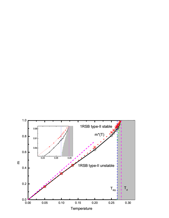
Figure 5: (Color Online) Same as Fig. 3, but for random regular graphs with vertex degree $K=20$. For $T>T_{RS}(20)=0.2674$ the RS mean-field solution is locally stable, while for $T<T_{d}(20)=T_{K}(20)=0.2793$ a non-trivial 1RSB mean-field solution appears at $m=1$. Notice that $T_{d}(20)>T_{RS}(20)$. The boundary line (which connected the $+$ symbols) between the white and the shaded regions marks the minimal value of $m$ below which the 1RSB solution has no non-trivial solutions. The insert is an enlarge of the main figure.

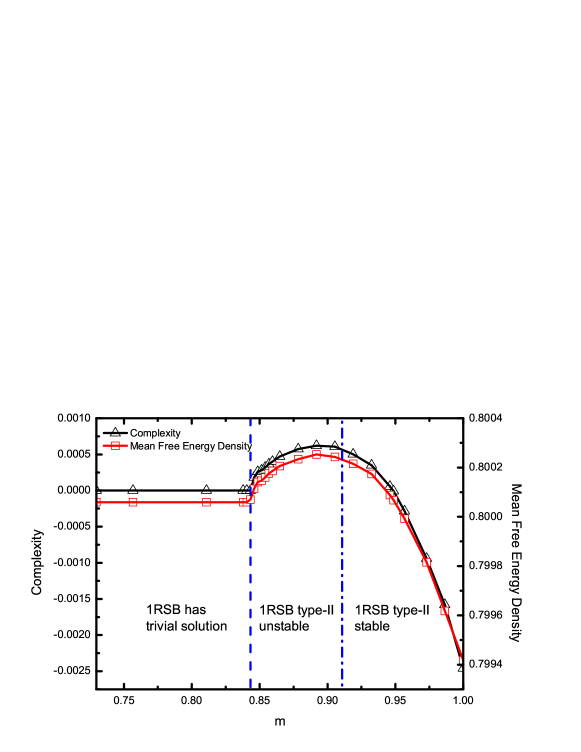
Figure 6: (Color Online) Complexity and mean free energy density at $T=0.2703$ for the VC problem on regular graphs with vertex degree $K=20$.

Figure 5 shows the phase diagram for the random regular graph vertex-cover problem with connectivity $K=20$. At this connectivity we obtain results that are qualitatively different from the results obtained for $K=5$ and $10$. The RS mean-field solution is locally stable when temperature $T>T_{RS}(20)=0.2674$. In this case, however, the dynamical transition temperature $T_{d}(K)$, which is determined as the maximal temperature at which a nontrivial 1RSB solution at $m=1$ exists, does not coincide with $T_{RS}(K)$. For $K=20$, $T_{d}(20)=0.2793$, and in the temperature range $T_{RS}(20)<T<T_{d}(20)$, non-trivial 1RSB solutions for the VC problem exist if the Parisi parameter $m$ is beyond the boundary line between the white and the gray region of Fig. 5. This result indicates that, in this temperature range, 1RSB solution and RS solution are both stable. However the existence of a non-trivial 1RSB solution at $m=1$ indicates that the RS solution is in fact not the physically meaningful one, as it does not describe the structure of the configuration space correctly.

As an example, for $K=20$ and $T=0.2703$, the complexity and the free energy density of the 1RSB solution of the VC problem are shown in Fig. 6 as a function of the Parisi parameter $m$. When $m<0.8459$, the 1RSB solution reduces to the RS solution, which has free energy density $f_{RS}\approx 0.80006$. A non-trivial 1RSB solution emerges for $m>0.8459$ and this 1RSB solution becomes type-II stable when $m>0.9108$. The complexity is a decreasing function of $m$ in the type-II stable region and it reaches zero at $m=0.9486$ (correspondingly, the free energy density of the dominating 1RSB macroscopic states is $f_{1RSB}\approx 0.80008$). Therefore the 1RSB free-energy density is only slightly larger than the RS free-energy density. For the whole temperature range $T_{RS}(20)<T<T_{d}(20)$ we have checked that the free energy density of the RS solution and that of the 1RSB solution at $m=m^{*}(T)$ are always very close to each other.

Figure 5 also demonstrates that, when the temperature $T$ is higher than $0.15$, the line $m^{*}(T)$, which corresponds to the dominating macroscopic states at each temperature, is located in the 1RSB type-II stable region. If the 1RSB solution is also type-I stable at $m\approx m^{*}(T)$ (which we have checked to be the case only for $T=0$, see the dashed line), then for $T>0.15$ the VC problem can be sufficiently described by the 1RSB solution without the need of further steps of replica-symmetry-breaking. Further work is obviously needed to study more closely the VC problem near the temperature $T_{RS}(K)$. For very low temperatures, however, the 1RSB solution will become type-II unstable.

IV.2.2 The case of random Erdös-Renyi graphs

Simulations on random ER graphs are technically more difficult, and therefore we have studied only the cases of mean vertex degree $c=5$ and $c=10$. For the case of $c=5$, results similar to Fig. 3 and Fig. 4 are obtained. The results for the case of $c=10$ are shown in Fig. 7. For this system, the 1RSB solution at $m=m^{*}(T)$ is type-II stable when $T>0.20$.

Figure 7: (Color Online) Phase diagram of the 1RSB solution of the VC problem on ER random graphs of mean vertex-degree $c=10$. The RS solution is stable for temperature $T>T_{RS}=T_{d}=T_{K}=0.25$. For this system the energetic zero-temperature 1RSB solution is type-I stable for $y\geq 0$.

IV.3 The stability thresholds of the zero-temperature energetic and entropic 1RSB cavity solution

As a check of the finite-temperature results, here we compare the low-temperature results with the results obtained directly at $T=0$. At the zero temperature limit, two types of 1RSB solutions can be written down. The energetic 1RSB solution Zhou (2003); Weigt and Zhou (2006), which neglects all the entropic effect of the VC problem, is much simplified. Both the type-I and type-II stability analysis of this solution can be performed. In this work, the type-II stability analysis is carried out through a bug proliferation simulation (the detailed mathematical formulas are given in Appendix B).

The entropic 1RSB solution takes into account both the energetic and the entropic effect and is numerically more involved. For the vertex-cover problem, following the entropic zero-temperature RS solution of Sec. III.2, we can develop the 1RSB solution by defining the 1RSB order parameter $Q_{j|i}(m_{j|i},r_{j|i})$. The iteration equation for $Q_{j|i}$ reads:

$$Q_{j|i}(m,r)=\frac{1}{Z_{j|i}}\prod\limits_{k\in\partial j\backslash i}\Biggl{[}\sum_{m_{k|j}}\int{\rm d}r_{k|j}Q_{k|j}(m_{k|j},r_{k|j})\Biggr{]}e^{-y\Delta E_{j|i}}\delta\bigl{(}m-m_{j|i}\bigr{)}\delta\bigl{(}r-r_{j|i}\bigr{)}\ ,$$ (49)

where $m_{j|i}$ and $r_{j|i}$ are expressed by Eq. (24) and Eq. (25).

When population dynamics is used to solve the entropic 1RSB equation Eq. (49), it is observed that, if the re-weighting parameter $y$ is lower than certain threshold value, the magnitudes of some of the $r_{j|i}$ parameters may increase continuously with iteration and eventually diverge. This divergence suggest that the zero-temperature entropic 1RSB solution is not stable. We use this divergence criterion to determine the type-II stability threshold of the zero-temperature entropic 1RSB solution.

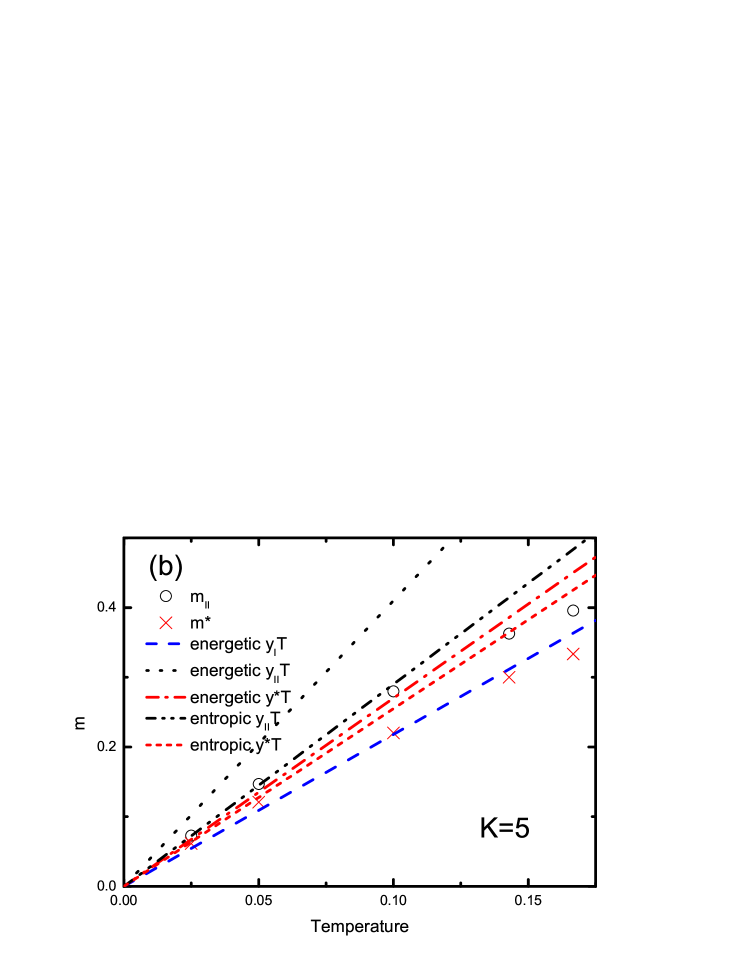
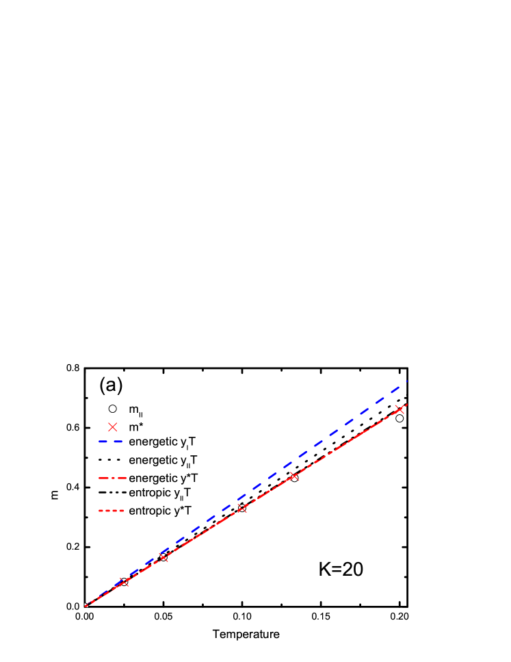
Figure 8 shows the stability boundaries of the finite temperature 1RSB solution, the energetic zero-temperature 1RSB solution, and the zero-temperature entropic 1RSB solution, for random regular graphs with $K=20$ and $K=5$. For both $K=20$ and $K=5$, the type-II stability threshold $y_{II}$ and value $y^{*}$ (determined by $\Sigma=0$) of the $T=0$ entropic 1RSB solution match the corresponding slops in the $T$-$m$ plane of the finite-temperature 1RSB solution. At $K=20$ the $T=0$ energetic 1RSB solution has the same value of $y^{*}$ as that of the entropic 1RSB solution; and the type-II stability threshold $y_{II}$ of the energetic 1RSB solution is very close to that of the entropic 1RSB solution.

The energetic 1RSB solution is stable for $y<y_{I}$. Since $y_{I}>y^{*}$ at $K=20$, the zero-temperature 1RSB solutions at are type-I stable $y=y^{*}$. However, $y_{I}<y^{*}$ for $K=5$, therefore the zero-temperature 1RSB solutions are type-I unstable at $y=y^{*}$. At this value of vertex connectivity, the type-II stability threshold $y_{II}$ as obtained for the 1RSB energetic solution and the 1RSB entropic solution are different.

Figure 8: (Color Online) Comparison of finite temperature results with the zero-temperature energetic and entropic 1RSB results for regular random graphs of vertex degree $K=20$ (a) and $K=5$ (b). Symbols are finite-temperature results. The blue dashed curve ($y_{I}T$ represent the slopes corresponding of type-I stability of the energetic zero temperature solutions. The energetic 1RSB solution is type-I stable when $y<y_{I}$. Black curves (dotted and dash dotted) represent the slopes corresponding to type-II stability of the (energetic and entropic) zero-temperature 1RSB solution. The 1RSB solution is type-II stable when $y>y_{II}$. Red curves (dash dotted and short dashed) represent the slopes corresponding to $y(\Sigma=0)$ of the (energetic and entropic) zero-temperature 1RSB solution.

V Conclusion

In summary, the vertex-cover problem on finite-connectivity random graphs were studied in this paper by finite-temperature cavity method at both the replica-symmetric and first-step replica-symmetry-breaking level, and the stability of these mean-field solutions were analyzed. We found that the local stability boundary $T_{RS}$ for the RS solution and the dynamical transition temperature $T_{d}$ show a re-entrant behavior with the connectivity both in the case of random regular graphs and Poisson random graphs: the threshold temperature $T_{RS}$ and $T_{d}$ first increases with connectivity and then decreases with connectivity. The reason for this re-entrant behavior (which is absent in the random $Q$-coloring problem Krzakala and Zdeborová (2007)) is not yet clear. For random regular graphs with a relatively large connectivity (e.g., $K=20$), there exists a temperature region in which both the RS solution and the 1RSB solutions with Parisi parameter $m$ close to unity are stable. This point deserves to be studied further on single graphs by the belief-propagation iteration process Yedidia et al. (2005); Hartmann and Weigt (2005) using different initial conditions. At relatively large connectivity, the VC problem at not too low temperatures may be sufficiently described by the 1RSB cavity solution without the need of further steps of replica-symmetry-breaking. But at temperature close to zero, more complicated mean-field solutions are needed Weigt and Hartmann (2001); Weigt and Zhou (2006); Zhou et al. (2007).

Appendix A Calculation of the dynamical transition temperature $T_{d}$

The dynamical transition temperature $T_{d}$ is defined as the highest temperature for the 1RSB cavity equation at Parisi parameter $m=1$ to have a non-trivial solution. To calculate $T_{d}$, one may solve the 1RSB equation Eq. (37) with $m=1$ using population dynamics, but numerically this is quite demanding, as population of populations is needed and different macrostates should be properly reweighted. It was first noticed in Ref. Mézard and Montanari (2006) that the 1RSB equation at $m=1$ may be solved without using populations of populations and reweighting of macrostates, and this possibility of simplification was exploited in various later studies Zdeborová and Krzakala (2007); Montanari et al. (2008); Zdeborová (2008); Zdeborová and M.Mézard (2008); Zdeborova and Mezard (2008). In this appendix, we follow Ref. Montanari et al. (2008) to solve Eq. (37) at $y=\beta$ (i.e., $m=1$).

At $m=1$ the mean cavity cover ratio $\overline{\pi}_{j|i}\equiv\int{\rm d}\pi_{j|i}Q_{j|i}(\pi_{j|i})\pi_{j|i}$ satisfies the following iteration equation

$$\overline{\pi}_{j|i}=\frac{e^{-\beta}}{e^{-\beta}+\prod_{k\in\partial j\backslash i}\overline{\pi}_{k|j}}\ ,$$ (50)

which has the same form as the RS iteration equation (9). Therefore, distribution of $\overline{\pi}_{j|i}$ among all the edges of the graph is given by $\mathcal{P}_{RS}$, see Eq. (12). Define $Q\left(\pi|\overline{\pi}\right)$ as the conditional probability that the cavity cover ratio is equal to $\pi$ when its mean value is $\overline{\pi}$. We have

$$Q\left(\pi|\overline{\pi}\right)\mathcal{P}_{RS}\left(\overline{\pi}\right)$$

$$\;\;=\int{\mathcal{D}}Q\mathcal{P}_{1RSB}\left[Q\right]Q\left(\pi\right)\delta\left(\overline{\pi}-\int d\pi Q\left(\pi\right)\pi\right)$$

$$\;\;=\sum\limits_{k=0}^{\infty}p_{nn}(k+1)\int\prod\limits_{j=1}^{k}{\mathcal{D}}Q_{j}\mathcal{P}_{1RSB}(Q_{j})\frac{\int\prod_{j=1}^{k}{\rm d}\pi_{j}Q_{j}(\pi_{j})(e^{-\beta}+\prod_{j}\pi_{j})}{e^{-\beta}+\prod_{j}\overline{\pi}_{j}}\delta\bigl{(}\pi-\mathcal{F}_{RS}(\{\pi_{j}\})\bigr{)}\delta\bigl{(}\overline{\pi}-\mathcal{F}_{RS}(\{\overline{\pi}_{j}\})\bigr{)}$$

$$\;\;=\sum\limits_{k=0}^{\infty}p_{nn}(k+1)\int\prod\limits_{j=1}^{k}{\rm d}\overline{\pi}_{j}{\mathcal{P}}_{RS}(\overline{\pi}_{j})\delta\bigl{(}\overline{\pi}-{\mathcal{F}}_{RS}(\{\overline{\pi}_{j}\})\bigr{)}\frac{\int\prod_{j}{\rm d}\pi_{j}{Q}_{j}(\pi_{j}|\overline{\pi}_{j})(e^{-\beta}+\prod_{j}\pi_{j})}{e^{-\beta}+\prod_{j}\overline{\pi}_{j}}\delta\bigl{(}\pi-\mathcal{F}_{RS}(\{\pi_{j}\})\bigr{)}\ .$$ (51)

In deriving Eq. (51), we have used the identity that ${Q}_{j}(\pi|\overline{\pi})\equiv\int{\mathcal{D}}Q_{j}\mathcal{P}_{1RSB}(Q_{j}|\overline{\pi})Q_{j}(\pi)$, with $\mathcal{P}_{1RSB}(Q_{j}|\overline{\pi})$ being the conditional probability of $Q_{j}$ given that the mean value of the cavity cover ratio is $\overline{\pi}$. $\mathcal{P}_{1RSB}(Q_{j}|\overline{\pi})$ is related to $\mathcal{P}_{1RSB}(Q_{j})$ by

$$\mathcal{P}_{1RSB}(Q_{j}|\overline{\pi})=\frac{\mathcal{P}_{1RSB}(Q_{j})\delta\bigl{(}\overline{\pi}-\int{\rm d}\pi Q_{j}(\pi)\pi\bigr{)}}{\int\mathcal{D}Q_{j}\mathcal{P}_{1RSB}(Q_{j})\delta\bigl{(}\overline{\pi}-\int{\rm d}\pi Q_{j}(\pi)\pi\bigr{)}}=\frac{\mathcal{P}_{1RSB}(Q_{j})\delta\bigl{(}\overline{\pi}-\int{\rm d}\pi Q_{j}(\pi)\pi\bigr{)}}{\mathcal{P}_{RS}(\overline{\pi})}\ .$$ (52)

To get rid of the reweighting term $(e^{-\beta}+\prod\limits_{j}\pi_{j})$ in Eq. (51), we define $Q_{\sigma_{j}}(\pi_{j}|\overline{\pi}_{j})$ as the conditional distribution that the cavity cover ratio of vertex $j$ is equal to $\pi_{j}$ given that the mean cavity cover ratio of vertex $j$ is $\overline{\pi}_{j}$ and that vertex $j$ is in the spin state $\sigma_{j}$. We have

$$Q_{\sigma_{j}}(\pi_{j}|\overline{\pi}_{j})\equiv\frac{\psi_{\sigma_{j}}Q(\pi_{j}|\overline{\pi}_{j})}{\overline{\psi}_{\sigma_{j}}}\ ,$$ (53)

where $\psi_{\sigma_{j}}=(1-\pi_{j})\delta_{\sigma_{j},1}+\pi_{j}\delta_{\sigma_{j},-1}$ is the probability distribution of $\sigma_{j}$, and $\overline{\psi}_{\sigma_{j}}=(1-\overline{\pi}_{j})\delta_{\sigma_{j},1}+\overline{\pi}_{j}\delta_{\sigma_{j},-1}$. Then Eq. (51) can be rewritten as

$$Q(\pi|\overline{\pi})\mathcal{P}_{RS}(\overline{\pi}) = \sum\limits_{k=0}^{\infty}p_{nn}(k+1)\int\prod\limits_{j=1}^{k}{\rm d}\overline{\pi}_{j}\mathcal{P}_{RS}(\overline{\pi}_{j})\delta(\overline{\pi}-\mathcal{F}_{RS}(\{\overline{\pi}_{j}\})$$ (54)

$$\times\sum\limits_{\sigma_{i}}\sum\limits_{\{\sigma_{j}\}}\frac{\delta_{\sigma_{i},-1}e^{-\beta}+\delta_{\sigma_{i},1}\prod_{j}\overline{\pi}_{j}\delta_{\sigma_{j},-1}}{e^{-\beta}+\prod_{j}\overline{\pi}_{j}}\times\int\prod\limits_{j=1}^{k}{\rm d}\pi_{j}Q_{\sigma_{j}}(\pi_{j}|\overline{\pi}_{j})\delta(\pi-\mathcal{F}_{RS}(\{\pi_{j}\}))\ .$$

From the above equation and the identity that

$$Q\left(\pi|\overline{\pi}\right)=\sum_{\sigma}\overline{\psi}_{\sigma}Q_{\sigma}\left(\pi|\bar{\pi}\right)\ ,$$ (55)

we obtain an iterative equation for $Q_{\sigma}(\pi|\overline{\pi})$:

$$\overline{\psi}_{\sigma}Q_{\sigma}\left(\pi|\overline{\pi}\right)\mathcal{P}_{RS}\left(\overline{\pi}\right) = \sum_{k=0}^{\infty}{p}_{nn}(k+1)\int\prod_{j=1}^{k}{\rm d}\overline{\pi}_{j}\mathcal{P}_{RS}\left(\overline{\pi}_{j}\right)\delta\left[\overline{\pi}-\mathcal{F}_{RS}\left(\left\{\overline{\pi}_{j}\right\}\right)\right]\times$$ (56)

$$\times\sum_{\left\{\sigma_{j}\right\}}\frac{e^{-\beta}\delta_{\sigma,-1}+\delta_{\sigma,1}\prod_{j}\overline{\pi}_{j}\delta_{\sigma_{j},-1}}{e^{-\beta}+\prod_{j}\overline{\pi}_{j}}\times\int\prod_{j=0}^{k}{\rm d}\pi_{j}Q_{\sigma}\left(\pi_{j}|\overline{\pi}_{j}\right)\delta\left[\pi-\mathcal{F}_{RS}\left(\left\{\pi_{j}\right\}\right)\right]\ .$$

According to Ref. Mézard and Montanari (2006), the 1RSB cavity equation Eq. (37) at $m=1$ has a non-trivial fixed point if Eq. (56) has a non-trivial solution with the initial conditions $Q_{1}(\pi=0|\overline{\pi})=1$ and $Q_{-1}(\pi=1|\overline{\pi})=1$, see also Refs. Montanari et al. (2008); Zdeborová (2008); Zdeborová and M.Mézard (2008); Zdeborova and Mezard (2008).

Appendix B energetic zero-temperature stability analysis

In this section, bug proliferation is used to analyze the type-II instability of 1-RSB solutions in vertex-cover problems. We introduce an message, the so-called warning $u_{j\rightarrow i}$ sent from vertex $j$ to a neighbor $i$. If the vertex $j$ is uncovered, it sends a warning $u_{j\rightarrow i}=1$ to $i$, otherwise $u_{j\rightarrow i}=0.$ To do survey propagation, $\pi^{(0)}_{i\mid j}$ ($\pi^{(1)}_{i\mid j}$) is used to represent the probability that vertex $i$ is always uncovered (covered) when $j$ is removed in a cluster. Similarly, $\pi^{(*)}_{i\mid j}$ is the probability that $i$ is unfrozen in the above situation.

$$\pi^{(0)}_{i\mid l} =c^{-1}_{i\mid l}\prod_{j\in N(i)\setminus l}(1-\pi^{(0)}_{j\mid i}),$$ (57)

$$\pi^{(*)}_{i\mid l} =c^{-1}_{i\mid l}e^{-y}\sum_{j\in N(i)\setminus l}\pi^{(0)}_{j\mid i}\prod_{j^{{}^{\prime}}\in N(i)\setminus\{j,l\}}(1-\pi^{(0)}_{j^{{}^{\prime}}\mid i}),$$ (58)

$$\pi^{(1)}_{i\mid l} =c^{-1}_{i\mid l}e^{-y}[1-\prod_{j\in N(i)\setminus l}(1-\pi^{(0)}_{j\mid i})-\sum_{j\in N(i)\setminus l}\pi^{(0)}_{j\mid i}\prod_{j^{{}^{\prime}}\in N(i)\setminus\{j,l\}}(1-\pi^{(0)}_{j^{{}^{\prime}}\mid i})],$$ (59)

$$c_{i\mid l} =e^{-y}[1-(1-e^{y})\prod_{j\in N(i)\setminus l}(1-\pi^{(0)}_{j\mid i}].$$ (60)

To analyze the type-II instability, a ”bug” is introduced and propagated on a graph. Here ”bug” means supposed that along edge $1$ the warning is $\beta_{1}$, we turn it to another type like $\beta_{0}$ with a very small probability $p^{1}_{\beta_{1}\rightarrow\beta_{0}}$. After one iteration, this will induce a new ”bug” $\gamma\rightarrow\delta$ on edge $l$ as an output and the probability of this situation is:

$$p^{l}_{\gamma\rightarrow\delta}=\frac{1}{Z}\sum_{\begin{array}[]{l}(\beta_{1},\cdots,\beta_{n})\rightarrow\gamma\\ (\beta_{0},\cdots,\beta_{n})\rightarrow\delta\end{array}}(p^{1}_{\beta_{1}\rightarrow\beta_{0}}\cdots p^{n}_{\beta_{n}})\exp{(-y\Delta E^{\prime})}$$ (61)

Thus we can define a matrix:

$$V_{\gamma\rightarrow\delta,\beta_{1}\rightarrow\beta_{0}}\equiv\frac{\partial p^{l}_{\gamma\rightarrow\delta}}{\partial p^{1}_{\beta_{1}\rightarrow\beta_{0}}}.$$ (62)

The bug is propagated on the graph and if it can proliferate the system is unstable. After $d$ times of iterations, absolutely the criterion of such an instability is determined by a product of $d$ matrices

$$C\cdot|\lambda_{MAX}|\equiv\mu_{d}$$ (63)

where $\lambda_{MAX}$ is the largest eigenvalue of matrix $V^{1}\ldots V^{d}$. If $\mu_{d}$ grows exponentially with $d$, the solution is unstable otherwise it is stable. Here the matrix $V$ is simply just $2\times 2$,

$$\left({\begin{array}[]{*{20}c}{V_{0\to 1,0\to 1}}&{V_{0\to 1,1\to 0}}\\ {V_{1\to 0,0\to 1}}&{V_{1\to 0,1\to 0}}\\ \end{array}}\right)$$ (64)

It is easy to get that:

$$V_{0\to 1,1\to 0} =\frac{e^{y}\prod_{k\in N(i)\setminus{j,l}}(1-\pi^{(0)}_{k\mid j})}{1-(1-e^{y})\prod_{k\in N(i)\setminus j}(1-\pi^{(0)}_{k\mid j})}$$ (65)

$$V_{1\to 0,0\to 1} =\frac{\prod_{k\in N(i)\setminus{j,l}}(1-\pi^{(0)}_{k\mid j})}{1-(1-e^{y})\prod_{k\in N(i)\setminus j}(1-\pi^{(0)}_{k\mid j})}$$ (66)

and $V_{0\to 1,0\to 1}=V_{1\to 0,1\to 0}=0$.

Solution about above equations and $\mu_{d}$ can be obtained through population dynamics. We have applied this analysis on the 1RSB solution of the vertex-cover problem with mean vertex degree $c=10$. The results are shown in the fig. 9. We estimate the threshold $y_{II}\approx 3.301$. Considering that the grand free-energy density reaches the peak at $y^{*}=3.13$, we therefore conclude that thermodynamics of the energetic zero-temperature 1RSB solution of the vertex-cover problem is unstable.

Figure 9: Stability of the 1RSB solution of random vertex-cover problem. $\ln\mu_{d}$ is plotted versus $d$ for different $y$. From top to bottom: 2, 3, 3.3, 3.5, 3.55 and the lines are the linear fits.

References

• Garey and Johnson (1979) M. Garey and D. S. Johnson, Computers and Intractability: A Guide to the Theory of NP-Completeness (Freeman, San Francisco, 1979).
• Hartmann and Weigt (2005) A. Hartmann and M. Weigt, Phase Transitions in Combinatorial Optimizatino Problems (Wiley-VCH, Berlin, 2005).
• Breitbart et al. (2001) Y. Breitbart, C. Chan, M. Garofalakis, R. Rastogi, and A. Silverschatz, Efficiently monitoring bandwidth and latency in IP networks (IEEE, Anchorage, Alaska, 2001).
• Park and Lee (2001) K. Park and H. Lee, On the effectiveness of route-based packet filtering for distributed DoS attack prevention in power-law internets (ACM, San Diego, California, 2001).
• Gomez-Gardenes et al. (2006) J. Gomez-Gardenes, P. Echenique, and y. Moreno, Eur. Phys. J. B 49, 259 (2006).
• Weigt and Hartmann (2001) M. Weigt and A. K. Hartmann, Phys. Rev. E 63, 056127 (2001).
• Zhou (2003) H. Zhou, Eur. Phys. J. B 32, 265 (2003).
• Weigt and Zhou (2006) M. Weigt and H. Zhou, Phys. Rev. E 74, 046110 (2006).
• Zhou (2005) H. Zhou, Phys. Rev. Lett. 94, 217203 (2005).
• Zhou et al. (2007) J. Zhou, H. Ma, and H. Zhou, J. Stat. Mech. L06001 (2007).
• Bauer and Golinelli (2001) M. Bauer and O. Golinelli, Eur. Phys. J. B 24, 339 (2001).
• Zhou and Zhou (2009) J. Zhou and H. Zhou, Phys. Rev. E 79, 020103(R) (2009).
• Mézard et al. (2002) M. Mézard, G. Parisi, and R. Zecchina, Science 297, 812 (2002).
• Mézard and Zecchina (2002) M. Mézard and R. Zecchina, Phys. Rev. E 66, 056126 (2002).
• Mézard and Parisi (2003) M. Mézard and G. Parisi, J. Stat. Phys. 111, 1 (2003).
• Krzakala and Zdeborová (2007) L. Krzakala and L. Zdeborová, Eur. Phys. Lett. 81, 57005 (2007).
• Montanari et al. (2008) A. Montanari, F. Ricci-Tesenghi, and G. Semerjian, J. Stat. Mech. P04004 (2008).
• Zdeborová and Krzakala (2007) L. Zdeborová and F. Krzakala, Phys. Rev. E 76, 031131 (2007).
• Zdeborová (2008) L. Zdeborová, arxiv:0806.4112 (2008).
• Montanari and Ricci-Tersenghi (2003) A. Montanari and F. Ricci-Tersenghi, Eur. Phys. J. B 33, 339 (2003).
• Montanari et al. (2004) A. Montanari, G. Parisi, and F. Ricci-Tersenghi, J. Phys. A: Math. Gen. 37, 2073 (2004).
• F. Krzakala et al. (2004) F. F. Krzakala, A. Pagnani, and M. Weigt, Phys. Rev. E 70, 046705 (2004).
• Bollobas (2001) B. Bollobas, Random Graphs (CUP, Cambridge, 2001).
• Mézard and Parisi (2001) M. Mézard and G. Parisi, Eur. Phys. J. B 20, 217 (2001).
• Chertkov and Chernyak (2006) M. Chertkov and V. Y. Chernyak, J. Stat. Mech. P06009 (2006).
• Zdeborová and Mézard (2006) L. Zdeborová and M. Mézard, J. Stat. Mech. p. P05003 (2006).
• Krzakala et al. (2007) F. Krzakala, A. Montanari, F. Ricci-Tersenghi, G. Semerjian, and L. Zdeborová, Proc. Natl. Acad. Sci. 104, 10318 (2007).
• Mézard and Montanari (2006) M. Mézard and A. Montanari, J. Stat. Phys. 124, 1317 (2006).
• Montanari and Semerjian (2006) A. Montanari and G. Semerjian, J. Stat. Phys. 124, 103 (2006).
• Zhou (2008) H. Zhou, Phys. Rev. E 77, 066102 (2008).
• Rivoire et al. (2004) O. Rivoire, G. Biroli, O. Martin, and M. Mézard, Eur. Phys. J. B 37, 55 (2004).
• Pagnani et al. (2003) A. Pagnani, G. Parisi, and M. Ratiéville, Phys. Rev. E 68, 046706 (2003).
• Yedidia et al. (2005) J. S. Yedidia, W. T. Freeman, and Y. Weiss, IEEE Trans. Inf. Theory 51, 2282 (2005).
• Zdeborová and M.Mézard (2008) L. Zdeborová and M.Mézard, Phys. Rev. Lett 101, 078702 (2008).
• Zdeborova and Mezard (2008) L. Zdeborova and M. Mezard, J. Stat. Mech. 12, 12004 (2008), URL http://www.iop.org/EJ/abstract/1742-5468/2008/12/P12004.