Converting Between Quadrilateral and Standard
Solution Sets in Normal Surface Theory

Abstract

The enumeration of normal surfaces is a crucial but very slow operation in algorithmic $3$–manifold topology. At the heart of this operation is a polytope vertex enumeration in a high-dimensional space (standard coordinates). Tollefson’s Q–theory speeds up this operation by using a much smaller space (quadrilateral coordinates), at the cost of a reduced solution set that might not always be sufficient for our needs. In this paper we present algorithms for converting between solution sets in quadrilateral and standard coordinates. As a consequence we obtain a new algorithm for enumerating all standard vertex normal surfaces, yielding both the speed of quadrilateral coordinates and the wider applicability of standard coordinates. Experimentation with the software package Regina shows this new algorithm to be extremely fast in practice, improving speed for large cases by factors from thousands up to millions.

1 Introduction

The theory of normal surfaces plays a pivotal role in algorithmic $3$–manifold topology. Introduced by Kneser [17] and further developed by Haken [10, 11], normal surfaces feature in key topological algorithms such as unknot recognition [10], $3$–sphere recognition [20, 21, 22], connected sum and JSJ decomposition [16], and testing for incompressible surfaces [14].

The beauty of normal surface theory is that it allows difficult topological questions to be transformed into straightforward linear programming problems, yielding algorithms that are well-suited for computer implementation. Unfortunately these linear programming problems can be extremely expensive computationally, which is what motivates the work described here.

Algorithms that employ normal surface theory typically operate as follows:

1. Begin with a compact $3$–manifold triangulation formed from $n$ tetrahedra;

2. Enumerate all vertex normal surfaces within this triangulation, as described below;

3. Search through this list for a surface of particular interest (such as an essential sphere for the connected sum decomposition algorithm, or an essential disc for the unknot recognition algorithm).

The linear programming problem (and often the bottleneck for the entire algorithm) appears in step (ii). It can be shown that the set of all normal surfaces within a triangulation is described by a polytope in a $7n$–dimensional vector space; step (ii) then requires us to enumerate the vertices of this polytope. The normal surfaces described by these vertices are called vertex normal surfaces.

The trouble with step (ii) is that the vertex enumeration algorithm can grow exponentially slow in $n$; moreover, this growth is unavoidable since the number of vertex normal surfaces can likewise grow exponentially large. As a result, normal surface algorithms are (at the present time) unusable for large triangulations.

Nevertheless, it is important to have these algorithms working as well as possible in practice. One significant advance in this regard was made by Tollefson [25], who showed that in certain cases, normal surface enumeration could be done in a much smaller vector space of dimension $3n$. This $3n$–dimensional space is called quadrilateral coordinates, and the resulting vertex normal surfaces (referred to by Tollefson as Q–vertex surfaces) form the quadrilateral solution set. For comparison, we refer to the original $7n$–dimensional space as standard coordinates and its vertex normal surfaces as the standard solution set. It is important to note that these solution sets are different (in fact we prove in Lemma 4.5 that one is essentially a proper subset of the other).

Practically speaking, quadrilateral coordinates are a significant improvement—although the running time remains exponential, experiments show that the enumeration of normal surfaces in quadrilateral coordinates runs orders of magnitude faster than in standard coordinates.

However, using quadrilateral coordinates can be problematic from a theoretical point of view. In the algorithm overview given earlier, step (iii) requires us to prove that, if an interesting surface exists, then it exists as a vertex normal surface. Such results are more difficult to prove in quadrilateral coordinates, largely because addition becomes a more complicated operation; in particular, useful properties of surfaces that are linear functionals in standard coordinates (such as as Euler characteristic) are no longer linear in quadrilateral coordinates. As a result, only a few results appear in the literature to show that quadrilateral coordinates can replace standard coordinates in certain topological algorithms.

The purpose of this paper is, in essence, to show that we can have our cake and eat it too. That is, we show that we can enumerate vertex normal surfaces in standard coordinates (thereby avoiding the theoretical problems of quadrilateral coordinates) by first constructing the quadrilateral solution set and then converting this into the standard solution set (thus avoiding the performance problems of standard coordinates). The conversion process is not trivial (and indeed forms the bulk of this paper), but it is found to be extremely fast in practice.

The key results in this paper are as follows:

• Algorithm 4.6, which gives a simple procedure for converting the standard solution set into the quadrilateral solution set;

• Algorithm 5.15, which gives a more complex procedure for converting the quadrilateral solution set into the standard solution set;

• Algorithm 5.17, which builds on these results to provide a new way of enumerating all vertex normal surfaces in standard coordinates, by going via quadrilateral coordinates as outlined above.

The final algorithm in this list (Algorithm 5.17) is the “end product” of this paper—it can be dropped into any high-level topological algorithm that requires the enumeration of vertex normal surfaces. Experimentation shows that this new algorithm runs orders of magnitude faster than the current state-of-the-art, with consistent improvements of the order of $10^{3}$–$10^{6}$ times the speed observed for large cases. Full details can be found in Section 6.

The remainder of this paper is structured as follows. Section 2 introduces the theory of normal surfaces, and defines the standard and quadrilateral solution sets precisely. In Section 3 we address the ambiguity inherent in quadrilateral coordinates by studying canonical surfaces and vectors. Sections 4 and 5 contain the main results, where we describe the conversion from standard to quadrilateral coordinates and quadrilateral to standard coordinates respectively. We finish in Section 6 with experimental testing that shows how well these new algorithms perform in practice.

Because this paper introduces a fair amount of notation, an appendix is included that lists the key symbols and where they are defined.

For researchers who wish to perform their own experiments, the three algorithms listed above have been implemented in version 4.6 of the software package Regina [3, 4].

Thanks must go to Ryan Budney and the University of Victoria, British Columbia for their hospitality during the development of this work, and to both RMIT University and the University of Melbourne for continuing to support the development of Regina. The author also thanks the Victorian Partnership for Advanced Computing for the use of their excellent computing resources.

2 Normal Surfaces

In this section we provide the essential definitions of normal surface theory, including both Haken’s original formulation (standard coordinates) and Tollefson’s normal surface Q–theory (quadrilateral coordinates).

We only present what is required to define the standard and quadrilateral solution sets. For a more thorough overview of normal surface theory the reader is referred to [12]; for further details on quadrilateral coordinates the reader is referred to Tollefson’s original paper [25].

Definition 2.1 (Triangulation).

A compact $3$–manifold triangulation is a finite collection of tetrahedra $\Delta_{1},\ldots,\Delta_{n}$, where some or all of the $4n$ tetrahedron faces are affinely identified in pairs, and where the resulting topological space is a compact $3$–manifold.

We allow different vertices of the same tetrahedron to be identified, and likewise with edges and faces (some authors refer to such structures as pseudo-triangulations or semi-simplicial triangulations). Any tetrahedron face that is not identified with some other tetrahedron face becomes part of the boundary of this $3$–manifold, and is referred to as a boundary face.

Each equivalence class of tetrahedron vertices under these identifications is called a vertex of the triangulation; likewise with edges and faces.

It should be noted that, according to this definition, the link of each vertex in the underlying $3$–manifold must be a disc or a $2$–sphere. This rules out the ideal triangulations of Thurston [23]; we discuss the reasons for this decision at the end of this section.

Definition 2.2 (Normal Surface).

Let $\mathcal{T}$ be a compact $3$–manifold triangulation, and let $\Delta$ be a tetrahedron of $\mathcal{T}$. A normal disc in $\Delta$ is a properly embedded disc in $\Delta$ which does not touch any vertices of $\Delta$, and whose boundary consists of either (i) three arcs running across three different faces of $\Delta$, or (ii) four arcs running across all four faces of $\Delta$. We refer to such discs as triangles and quadrilaterals respectively.

There are seven different types of normal disc in a tetrahedron, defined by the choice of which tetrahedron edges a disc intersects. These include (i) four triangle types, each surrounding a single vertex of $\Delta$, and (ii) three quadrilateral types, each separating a single pair of opposite edges of $\Delta$. All seven disc types are illustrated in Figure 1.

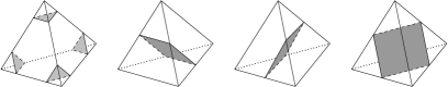
Figure 1: The seven different types of normal disc in a tetrahedron

An embedded normal surface in the triangulation $\mathcal{T}$ is a properly embedded surface that intersects each tetrahedron of $\mathcal{T}$ in a (possibly empty) collection of disjoint normal discs. Here we allow both disconnected surfaces and the empty surface.

We consider two normal surfaces identical if they are related by a normal isotopy, i.e., an ambient isotopy that preserves each simplex of $\mathcal{T}$.

We divert briefly to define a particular class of normal surface that plays an important role in the relationship between standard and quadrilateral coordinates.

Definition 2.3 (Vertex Link).

Let $\mathcal{T}$ be a compact $3$–manifold triangulation, and let $V$ be some vertex of $\mathcal{T}$. We define the vertex link of $V$, denoted $\ell(V)$, to be the normal surface that appears at the frontier of a small regular neighbourhood of $V$. In particular, $\ell(V)$ contains one copy of each triangular disc type surrounding $V$, and contains no other normal discs at all.

Here we follow the nomenclature of Jaco and Rubinstein [15]; in particular, Definition 2.3 is not the same as the combinatorial link in a simplicial complex. Tollefson refers to vertex links as trivial surfaces [25].

Note that Definition 2.1 implies that $\ell(V)$ is a disc or a $2$–sphere (according to whether or not $V$ is on the boundary of the $3$–manifold). In the case where $\mathcal{T}$ is a one-vertex triangulation, the normal surface $\ell(V)$ contains precisely one copy of every triangular disc type in the triangulation, and no other normal discs.

At this point the theory of normal surfaces moves into linear algebra, whereupon we must choose between the formulation of Haken (standard coordinates) or Tollefson (quadrilateral coordinates). In the text that follows we outline both formulations side by side.

Definition 2.4 (Vector Representations).

Let $\mathcal{T}$ be a compact $3$–manifold triangulation built from the $n$ tetrahedra $\Delta_{1},\ldots,\Delta_{n}$, and let $S$ be an embedded normal surface in $\mathcal{T}$.

Consider the individual normal discs that form the surface $S$. Let $t_{i,j}$ denote the number of triangular discs of the $j$th type in $\Delta_{i}$ ($j=1,2,3,4$), and let $q_{i,k}$ denote the number of quadrilateral discs of the $k$th type in $\Delta_{i}$ ($k=1,2,3$).

Then the standard vector representation of $S$, denoted $\mathbf{v}(S)$, is the $7n$–dimensional vector

$$\mathbf{v}(S)~{}=\,(~{} t_{1,1},t_{1,2},t_{1,3},t_{1,4},\ q_{1,1},q_{1,2} ,q_{1,3}\ ;$$

$$t_{2,1},t_{2,2},t_{2,3},t_{2,4},\ q_{2,1},q_{2,2} ,q_{2,3}\ ;$$

$$\ldots ,q_{n,3}\ ),$$

and the quadrilateral vector representation of $S$, denoted $\mathbf{q}(S)$, is the $3n$–dimensional vector

$$\mathbf{q}(S)~{}=\,(~{}q_{1,1},q_{1,2},q_{1,3}\ ;\ q_{2,1},q_{2,2},q_{2,3}\ ;\ \ldots,q_{n,3}\ ).$$

When we are working with standard vector representations in $\R^{7n}$ we say we are working in standard coordinates. Likewise, when working with quadrilateral vector representations in $\R^{3n}$ we say we are working in quadrilateral coordinates.

It turns out that, if we ignore vertex links, then the vector representations contain enough information to completely reconstruct a normal surface. The results, due to Haken [10] and Tollefson [25], are as follows.

Lemma 2.5.

Consider two embedded normal surfaces $S$ and $T$ within some compact $3$–manifold triangulation.

• The standard vector representations of $S$ and $T$ are equal, that is, $\mathbf{v}(S)=\mathbf{v}(T)$, if and only if surfaces $S$ and $T$ are identical.

• The quadrilateral vector representations of $S$ and $T$ are equal, that is, $\mathbf{q}(S)=\mathbf{q}(T)$, if and only if (i) $S$ and $T$ are identical, or (ii) $S$ and $T$ differ only by adding or removing vertex linking components.

Although every embedded normal surface has a standard and quadrilateral vector representation, there are many vectors in $\R^{7n}$ and $\R^{3n}$ respectively that do not represent any normal surface at all. Haken [10] and Tollefson [25] completely characterise which vectors represent embedded normal surfaces, using the concept of admissible vectors. We build up a definition of this concept now, and then present the full characterisation results of Haken and Tollefson in Theorem 2.10.

Definition 2.6 (Standard Matching Equations).

Let $\mathcal{T}$ be a compact $3$–manifold triangulation built from the $n$ tetrahedra $\Delta_{1},\ldots,\Delta_{n}$, and consider some $7n$–dimensional vector $\mathbf{v}=\left(t_{1,1},t_{1,2},t_{1,3},t_{1,4},q_{1,1},q_{1,2},q_{1,3};\ldots,q_{n,3}\right)$. For each non-boundary face $F$ of $\mathcal{T}$ and each edge $e$ of the face $F$, we obtain an equation as follows.

In essence, our equation states that we must be able to match the normal discs on one side of $F$ with the normal discs on the other. To express this formally, let $\Delta_{i}$ and $\Delta_{j}$ be the two tetrahedra joined along face $F$. In each tetrahedron $\Delta_{i}$ and $\Delta_{j}$ there is precisely one triangle type and one quadrilateral type that meets face $F$ in an arc parallel to $e$; let these be described by the coordinates $t_{i,a}$ and $q_{i,b}$ in $\Delta_{i}$ and $t_{j,c}$ and $q_{j,d}$ in $\Delta_{j}$. Our equation is then

$$t_{i,a}+q_{i,b}=t_{j,c}+q_{j,d}.$$

The set of all such equations is called the set of standard matching equations for $\mathcal{T}$.

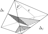
Figure 2: An example of the standard matching equations

Note that if $\mathcal{T}$ has $f$ non-boundary faces then there are $3f$ such equations in total; in particular, if $\mathcal{T}$ has no boundary at all then there are $6n$ standard matching equations. Figure 2 shows an illustration of one such equation; here we have one triangle and one quadrilateral in $\Delta_{i}$ meeting two triangles in $\Delta_{j}$, giving $(t_{i,a}+q_{i,b}=1+1)=(t_{j,c}+q_{j,d}=2+0)$.

Definition 2.7 (Quadrilateral Matching Equations).

Let $\mathcal{T}$ be a compact $3$–manifold triangulation built from the $n$ tetrahedra $\Delta_{1},\ldots,\Delta_{n}$, and consider some $3n$–dimensional vector $\mathbf{q}=\left(q_{1,1},q_{1,2},q_{1,3};\ldots,q_{n,3}\right)$. For each non-boundary edge $e$ of $\mathcal{T}$, we obtain an equation as follows.

Consider the tetrahedra containing edge $e$; these are arranged in a cycle around $e$ as illustrated in Figure 3. Choose an arbitrary direction around this cycle, and arbitrarily label the two ends of $e$ as upper and lower.

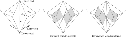
Figure 3: Building the quadrilateral matching equations

Within each of these tetrahedra, there are two quadrilateral types that meet edge $e$: the upward quadrilaterals, which rise from the lower end of $e$ to the upper end as we move around the cycle, and the downward quadrilaterals, which fall in the opposite direction. These are again illustrated in Figure 3.

We can now create an equation from edge $e$ as follows. Let the tetrahedra containing $e$ be $\Delta_{i_{1}},\Delta_{i_{2}},\ldots,\Delta_{i_{k}}$, let the coordinates corresponding to the upward quadrilateral types be $q_{i_{1},u_{1}},q_{i_{2},u_{2}},\ldots,q_{i_{k},u_{k}}$, and let the coordinates corresponding to the downward quadrilateral types be $q_{i_{1},d_{1}},q_{i_{2},d_{2}},\ldots,q_{i_{k},d_{k}}$. Then we obtain the equation

$$q_{i_{1},u_{1}}+q_{i_{2},u_{2}}+\ldots+q_{i_{k},u_{k}}=q_{i_{1},d_{1}}+q_{i_{2},d_{2}}+\ldots+q_{i_{k},d_{k}}.$$

The set of all such equations is called the set of quadrilateral matching equations for $\mathcal{T}$.

We will see that both the standard and quadrilateral matching equations form necessary but not sufficient conditions for a non-negative integer vector to represent an embedded normal surface. We still need one more set of constraints, which we define as follows.

Definition 2.8 (Quadrilateral Constraints).

Let $\mathcal{T}$ be a compact $3$–manifold triangulation built from the $n$ tetrahedra $\Delta_{1},\ldots,\Delta_{n}$, and let $\mathbf{w}$ be either a $7n$–dimensional vector of the form $\left(t_{1,1},t_{1,2},t_{1,3},t_{1,4},q_{1,1},q_{1,2},q_{1,3};\ldots,q_{n,3}\right)$, or a $3n$–dimensional vector of the form $\left(q_{1,1},q_{1,2},q_{1,3};\ldots,q_{n,3}\right)$.

Then $\mathbf{w}$ satisfies the quadrilateral constraints if, for each tetrahedron $\Delta_{i}$, at most of one of the quadrilateral coordinates $q_{i,1}$, $q_{i,2}$ and $q_{i,3}$ is non-zero.

The quadrilateral constraints arise because any two quadrilaterals of different types within the same tetrahedron must intersect, yet embedded normal surfaces cannot have self-intersections. We have now gathered enough conditions for the complete characterisation results of Haken [10] and Tollefson [25], which we reproduce in Definition 2.9 and Theorem 2.10.

Definition 2.9 (Admissible Vector).

Let $\mathcal{T}$ be a compact $3$–manifold triangulation built from $n$ tetrahedra. A ($7n$ or $3n$)–dimensional vector is called admissible if (i) its entries are all non-negative, (ii) it satisfies the (standard or quadrilateral) matching equations for $\mathcal{T}$, and (iii) it satisfies the quadrilateral constraints for $\mathcal{T}$.

Theorem 2.10.

Let $\mathcal{T}$ be a compact $3$–manifold triangulation built from $n$ tetrahedra, and let $\mathbf{w}$ be a ($7n$ or $3n$)–dimensional vector of integers. Then $\mathbf{w}$ is the (standard or quadrilateral) vector representation of an embedded normal surface in $\mathcal{T}$ if and only if $\mathbf{w}$ is admissible.

Although we can now reduce normal surfaces to vectors in $\R^{7n}$ or $\R^{3n}$, we still have infinitely many surfaces to search through if we are seeking an “interesting” surface, such as an essential $2$–sphere or an incompressible surface. The following series of definitions, due to Jaco and Oertel [14], allow us to reduce such searches to finite problems by restricting our attention to what are known as vertex normal surfaces.

Definition 2.11 (Projective Solution Space).

For any dimension $d$, we define the following regions in $\R^{d}$:

• The non-negative orthant $O^{d}$ is the region in $\R^{d}$ in which all coordinates are non-negative; that is, $O^{d}=\{\mathbf{x}\in\R^{d}\,|\,x_{i}\geq 0\ \forall i\}$.

• The projective hyperplane $J^{d}$ is the hyperplane in $\R^{d}$ where all coordinates sum to 1; that is, $J^{d}=\{\mathbf{x}\in\R^{d}\,|\,\sum x_{i}=1\}$.

Note that the intersection $O^{d}\cap J^{d}$ is the unit simplex in $\R^{d}$.

Let $\mathcal{T}$ be a compact $3$–manifold triangulation built from $n$ tetrahedra. The standard projective solution space for $\mathcal{T}$, denoted $\mathscr{S}(\mathcal{T})$, is the region in $\R^{7n}$ consisting of all points in $O^{7n}\cap J^{7n}$ that satisfy the standard matching equations. Likewise, the quadrilateral projective solution space for $\mathcal{T}$, denoted $\mathscr{Q}(\mathcal{T})$, is the region in $\R^{3n}$ consisting of all points in $O^{3n}\cap J^{3n}$ that satisfy the quadrilateral matching equations.

Since each $O^{d}\cap J^{d}$ is the unit simplex and the matching equations are both linear and rational, it follows that the standard and quadrilateral projective solution spaces are (finite) convex rational polytopes in $\R^{7n}$ and $\R^{3n}$ respectively.

It is clear from Theorem 2.10 that the non-zero vectors in $\R^{7n}$ or $\R^{3n}$ that represent embedded normal surfaces are precisely those positive multiples of points in $\mathscr{S}(\mathcal{T})$ or $\mathscr{Q}(\mathcal{T})$ that (i) are integer vectors, and (ii) satisfy the quadrilateral constraints.

Definition 2.12 (Projective Image).

Suppose that $\mathbf{x}\in\R^{d}$ is not the zero vector. We define the projective image of $\mathbf{x}$, denoted $\overline{\mathbf{x}}$, to be the vector $\mathbf{x}/\sum x_{i}$. In other words, $\overline{\mathbf{x}}$ is the (unique) multiple of $\mathbf{x}$ that lies in the projective hyperplane $J^{d}$.

To avoid complications with vertex links and the empty surface, we define the projective image of the zero vector to be the zero vector. That is, $\overline{\mathbf{0}}=\mathbf{0}$ (which does not lie in the projective hyperplane $J^{d}$).

Let $S$ be an embedded normal surface in some triangulation $\mathcal{T}$. To keep our notation clean, we write the projective images of the vector representations $\mathbf{v}(S)$ and $\mathbf{q}(S)$ as $\overline{\mathbf{v}}(S)$ and $\overline{\mathbf{q}}(S)$ respectively.

Definition 2.13 (Vertex Normal Surface).

Let $\mathcal{T}$ be a compact $3$–manifold triangulation built from $n$ tetrahedra, and let $S$ be an embedded normal surface in $\mathcal{T}$. We call $S$ a standard vertex normal surface if and only if $\overline{\mathbf{v}}(S)$ (the projective image of the standard vector representation of $S$) is a vertex of the polytope $\mathscr{S}(\mathcal{T})$. Likewise, we call $S$ a quadrilateral vertex normal surface if and only if $\overline{\mathbf{q}}(S)$ is a vertex of the polytope $\mathscr{Q}(\mathcal{T})$.

Although vertex normal surfaces correspond to vertices of the projective solution space, this correspondence does not always work in the other direction. Instead we must restrict our attention to vectors that satisfy the quadrilateral constraints.

Definition 2.14 (Solution Sets).

Let $\mathcal{T}$ be a compact $3$–manifold triangulation built from $n$ tetrahedra. The standard solution set for $\mathcal{T}$ is the (finite) set of all vertices of the polytope $\mathscr{S}(\mathcal{T})$ that satisfy the quadrilateral constraints. Likewise, the quadrilateral solution set for $\mathcal{T}$ is the (finite) set of all vertices of the polytope $\mathscr{Q}(\mathcal{T})$ that satisfy the quadrilateral constraints.

The correspondence between solution sets and vertex normal surfaces is now an immediate consequence of Theorem 2.10 and the fact that each projective solution space is a rational polytope:

Corollary 2.15.

Let $\mathcal{T}$ be a compact $3$–manifold triangulation built from $n$ tetrahedra, and let $\mathbf{w}$ be a ($7n$ or $3n$)–dimensional vector. Then $\mathbf{w}$ is the projective image of the vector representation for a (standard or quadrilateral) vertex normal surface if and only if $\mathbf{w}$ is in the (standard or quadrilateral) solution set.

We return now to the overview of a “typical normal surface algorithm” as given in Section 1. Such algorithms typically work because we can prove that, if a $3$–manifold triangulation contains an “interesting” surface, then it contains an interesting vertex normal surface. Examples of such theorems include:

• Jaco and Oertel [14] show that, if a closed irreducible $3$–manifold triangulation contains a two-sided incompressible surface, then such a surface exists as a standard vertex normal surface. Jaco and Tollefson [16] extend this result to bounded manifolds, and Tollefson [25] shows that such a surface must also exist as a quadrilateral vertex normal surface.

• Jaco and Tollefson [16] prove similar results for essential spheres in closed $3$–manifolds and essential compression discs in bounded irreducible $3$–manifolds; in particular, they show that if such a surface exists then one can be found amongst the standard vertex normal surfaces. With these results, they build algorithms to solve problems such as connected sum decomposition, JSJ decomposition and unknot recognition.

We can therefore build such an algorithm by constructing the standard or quadrilateral solution set for our triangulation, and then searching through the solutions for one that scales to an “interesting” normal surface.

The construction of the solution sets is, though finite, an exponentially slow procedure in the number of tetrahedra $n$. The best known algorithm to date is described in [5]; it is essentially a variant of the double description method of Motzkin et al. [19], modified in several ways to exploit the quadrilateral constraints for greater speed and lower memory consumption.

The remainder of this paper is concerned mainly with the conversion between the standard solution set and the quadrilateral solution set. Upon establishing conversion algorithms in both directions (Algorithms 4.6 and 5.15), we finish with a new algorithm for constructing the standard solution set (Algorithm 5.17) that is orders of magnitude faster than the current state-of-the-art.

We conclude this section with a brief discussion of ideal triangulations. These triangulations, due to Thurston [23], include vertices whose links are neither $2$–spheres nor discs, but rather closed surfaces with genus (such as tori or Klein bottles). By removing these vertices (and only these vertices), we obtain a triangulation of a non-compact $3$–manifold. One of the most well-known ideal triangulations is the two-tetrahedron triangulation of the figure eight knot complement, discussed in detail in [18].

Quadrilateral coordinates play a special role in ideal triangulations—they allow us to describe spun normal surfaces, which contain infinitely many triangular discs spiralling in towards the high-genus vertices. Such surfaces cannot be represented in standard coordinates at all, which is why we must restrict our attention in this paper to compact $3$–manifold triangulations. The reader is referred to Tillmann [24] for a thorough overview of spun normal surfaces.

3 Canonical Surfaces and Vectors

Although our eventual goal is to construct algorithms for converting between the standard and quadrilateral solution sets, we begin in this section with the more modest aim of converting between standard and quadrilateral vectors.

One complication we face is that, whereas vectors in standard coordinates represent unique normal surfaces, vectors in quadrilateral coordinates do not (Lemma 2.5). We work around this uniqueness problem by introducing the notion of canonical surfaces and canonical vectors in standard coordinates. Although this allows us to map vectors in quadrilateral coordinates to unique canonical vectors in standard coordinates and unique canonical surfaces, we will find that these maps are not as well-behaved as we might like them to be.

The structure of this section is as follows. We first define canonical surfaces and canonical vectors and examine some of their basic properties. Following this we study several additional maps between both surfaces and vectors; amongst these maps are the quadrilateral projection $\pi\co\R^{7n}\to\R^{3n}$ and the canonical extension $\varepsilon\co\R^{3n}\to\R^{7n}$, which convert back and forth between vectors in standard and quadrilateral coordinates. We finish the section with Algorithm 3.12, which shows how these conversions can be performed in as fast a time complexity as possible.

Throughout this section, we assume that we are working with a compact $3$–manifold triangulation $\mathcal{T}$ built from $n$ tetrahedra. We also allow a little flexibility with our notation: the expression $\ell(V)$ will be used to refer to both the vertex linking surface surrounding $V$ (as presented in Definition 2.3) and also its standard vector representation in $\R^{7n}$.

Definition 3.1 (Canonical Normal Surface).

A canonical normal surface in the triangulation $\mathcal{T}$ is an embedded normal surface that does not contain any vertex linking components.

The purpose of this definition is to resolve the ambiguities inherent in quadrilateral coordinates. In particular, it gives us the following uniqueness properties, which follow immediately from Lemma 2.5 and Theorem 2.10:

Lemma 3.2.

Let $S$ and $T$ be canonical normal surfaces within the triangulation $\mathcal{T}$. Then the quadrilateral vector representations of $S$ and $T$ are equal, that is, $\mathbf{q}(S)=\mathbf{q}(T)$, if and only if surfaces $S$ and $T$ are identical.

Lemma 3.3.

Let $\mathbf{w}$ be a $3n$–dimensional vector of integers. Then $\mathbf{w}$ is the quadrilateral vector representation of a canonical normal surface in $\mathcal{T}$ if and only if $\mathbf{w}$ is admissible. Moreover, this canonical normal surface is unique.

Instead of thinking of canonical surfaces as having no vertex links, we can instead think of them as surfaces where it is impossible to remove a vertex link. With this in mind, we extend the concept from surfaces to vectors as follows.

Definition 3.4 (Canonical Vector).

Let $\mathbf{w}$ be any vector in $\R^{7n}$ (i.e., in standard coordinates). We call $\mathbf{w}$ a canonical vector if and only if (i) all triangular coordinates of $\mathbf{w}$ are non-negative, but (ii) if we subtract $\epsilon\ell(V)$ for any $\epsilon>0$ and any vertex link $\ell(V)$ then some triangular coordinate of $\mathbf{w}$ must become negative.

In other words, for each vertex $V$ of the triangulation $\mathcal{T}$, the following property must hold. Let $t_{i_{1},j_{1}},t_{i_{2},j_{2}},\ldots,t_{i_{k},j_{k}}$ be the coordinates in $\mathbf{w}$ corresponding to the triangular normal discs surrounding $V$. Then all of $t_{i_{1},j_{1}},t_{i_{2},j_{2}},\ldots,t_{i_{k},j_{k}}$ are at least zero, and at least one of these coordinates is equal to zero.

Essentially this definition states that (i) $\mathbf{w}$ might be admissible (having non-negative triangular coordinates), but (ii) $\mathbf{w}-\epsilon\ell(V)$ can never be admissible.

We have already established two bijections between surfaces and vectors: Theorem 2.10 shows a bijection between embedded normal surfaces and admissible integer vectors in $\R^{7n}$, and Lemma 3.3 shows a bijection between canonical normal surfaces and admissible integer vectors in $\R^{3n}$. We can now extend this list with a bijection between canonical normal surfaces and admissible canonical integer vectors in $\R^{7n}$.

Lemma 3.5.

The standard vector representation of a canonical normal surface is a canonical vector in $\R^{7n}$. Conversely, every admissible canonical integer vector in $\R^{7n}$ is the standard vector representation of a (unique) canonical normal surface.

Proof.

This result follows immediately from Theorem 2.10 by observing that, if an admissible integer vector $\mathbf{w}\in\R^{7n}$ is not canonical, then all of the triangular coordinates surrounding some vertex $V$ are $\geq 1$, and so $\mathbf{w}=\ell(V)+\mathbf{w^{\prime}}$ for some other admissible integer vector $\mathbf{w^{\prime}}$. ∎

We can observe that, if we restrict our attention to admissible integer vectors, then we have bijections between (i) canonical vectors in standard coordinates and canonical surfaces, and (ii) vectors in quadrilateral coordinates and canonical surfaces. It follows then that we must have a bijection between canonical vectors in standard coordinates and vectors in quadrilateral coordinates; that is, a method for converting between coordinate systems. We develop this idea further in Definition 3.10.

Although the “canonical” property gives us uniqueness results and bijections that we did not have before, it is not particularly well-behaved. In particular, it is clear from Definition 3.4 that this property is preserved under scalar multiplication but not necessarily under addition. However, we can salvage the situation a little as seen in the following result.

Lemma 3.6.

If $\mathbf{w}\in\R^{7n}$ is a canonical vector then so is $\lambda\mathbf{w}$ for any $\lambda>0$. Likewise, if $\mathbf{w}\in\R^{7n}$ is an admissible canonical vector then so is $\lambda\mathbf{w}$ for any $\lambda>0$. Finally, if $\mathbf{w}=\mathbf{x}+\mathbf{y}$ for admissible vectors $\mathbf{w},\mathbf{x},\mathbf{y}\in\R^{7n}$ and $\mathbf{w}$ is canonical then so are $\mathbf{x}$ and $\mathbf{y}$.

Proof.

This follows immediately from Definition 3.4 and the fact that the matching equations are invariant under scalar multiplication. ∎

We proceed now to define several mappings that express the relationships between canonical surfaces, non-canonical surfaces, vectors in standard coordinates and vectors in quadrilateral coordinates. Lemma 3.11 summarises the interplay between these relationships. We begin by presenting notation for the domains and ranges of these functions.

Notation 3.7.

Let $\mathbb{S}$ denote the set of all embedded normal surfaces (up to normal isotopy), and let $\mathbb{S}_{c}\subset\mathbb{S}$ denote the set of all canonical normal surfaces. Let $\R_{a}^{7n}$ and $\R_{a}^{3n}$ denote the set of all admissible vectors in $7n$ and $3n$ dimensions respectively, and let $\R_{a,c}^{7n}\subset\R_{a}^{7n}$ denote the set of all admissible canonical vectors in $7n$ dimensions. Likewise, let $\Z_{a}^{7n}$ and $\Z_{a}^{3n}$ denote the set of all admissible integer vectors in $7n$ and $3n$ dimensions respectively, and let $\Z_{a,c}^{7n}\subset\Z_{a}^{7n}$ denote the set of all admissible canonical integer vectors in $7n$ dimensions.

It follows then that standard vector representation is a bijection $\mathbf{v}\co\mathbb{S}\to\Z_{a}^{7n}$ that takes the subset $\mathbb{S}_{c}\subset\mathbb{S}$ to the subset $\Z_{a,c}^{7n}\subset\Z_{a}^{7n}$. Likewise, quadrilateral vector representation is a many-to-one function $\mathbf{q}\co\mathbb{S}\to\Z_{a}^{3n}$ that becomes a bijection when restricted to $\mathbb{S}_{c}$.

Definition 3.8 (Represented Surface).

Let $\mathbf{w}$ be an admissible integer vector in $\R^{7n}$. Then the represented surface of $\mathbf{w}$, denoted $\sigma_{v}(\mathbf{w})$, is the unique embedded normal surface with standard vector representation $\mathbf{w}$ (as noted in Theorem 2.10). Thus $\sigma_{v}\co\Z_{a}^{7n}\to\mathbb{S}$ is the inverse function to $\mathbf{v}\co\mathbb{S}\to\Z_{a}^{7n}$.

Likewise, let $\mathbf{w}$ be an admissible integer vector in $\R^{3n}$. Then the represented surface of $\mathbf{w}$, denoted $\sigma_{q}(\mathbf{w})$, is the unique canonical normal surface with quadrilateral vector representation $\mathbf{w}$ (as noted in Lemma 3.3). Thus $\sigma_{q}\co\Z_{a}^{3n}\to\mathbb{S}_{c}$ is the inverse function to the restriction $\mathbf{q}\co\mathbb{S}_{c}\to\Z_{a}^{3n}$.

Definition 3.9 (Canonical Part).

Let $S$ be an embedded normal surface within the triangulation $\mathcal{T}$. The canonical part of $S$, denoted $\kappa_{s}(S)$, is the canonical normal surface obtained by removing all vertex linking components from $S$. It follows that $\kappa_{s}$ is a function $\kappa_{s}\co\mathbb{S}\to\mathbb{S}_{c}$ whose restriction to $\mathbb{S}_{c}$ is the identity.

Similarly, let $\mathbf{w}$ be any vector in $\R^{7n}$. The canonical part of $\mathbf{w}$, denoted $\kappa_{v}(\mathbf{w})$, is the unique canonical vector that can be obtained from $\mathbf{w}$ by adding and/or subtracting scalar multiples of vertex links. It follows that, if we restrict our attention to admissible vectors, then $\kappa_{v}$ is a function $\kappa_{v}\co\R_{a}^{7n}\to\R_{a,c}^{7n}$ whose restriction to $\R_{a,c}^{7n}$ is the identity.

The canonical part of a vector $\mathbf{w}\in\R^{7n}$ can be constructed as follows. Let the vertices of the triangulation be $V_{1},\ldots,V_{m}$, and for each $i$ let $\lambda_{i}$ be the minimum of all triangular coordinates in $\mathbf{w}$ that correspond to triangular normal discs surrounding $V_{i}$ (so $\mathbf{w}$ is canonical if and only if every $\lambda_{i}=0$). Then $\kappa_{v}(\mathbf{w})=\mathbf{w}-\lambda_{1}\ell(V_{1})-\ldots-\lambda_{m}\ell(V_{m})$.

We now come to the point of defining conversion functions between vectors in standard coordinates and vectors in quadrilateral coordinates.

Definition 3.10 (Projection and Extension).

Let $\mathbf{w}\in\R^{7n}$ be any vector in standard coordinates; recall that the $7n$ coordinates of $\mathbf{w}$ correspond to $3n$ quadrilateral disc types and $4n$ triangular disc types. The quadrilateral projection of $\mathbf{w}$, denoted $\pi(\mathbf{w})$, is defined to be the vector in $\R^{3n}$ consisting of only the $3n$ quadrilateral coordinates for $\mathbf{w}$. That is, if

$$\mathbf{w}~{}=\,(~{} t_{1,1},t_{1,2},t_{1,3},t_{1,4},\ q_{1,1},q_{1,2} ,q_{1,3}\ ;$$

$$t_{2,1},t_{2,2},t_{2,3},t_{2,4},\ q_{2,1},q_{2,2} ,q_{2,3}\ ;$$

$$\ldots ,q_{n,3}\ )\in\R^{7n},$$

then

$$\pi(\mathbf{w})~{}=\,(~{}q_{1,1},q_{1,2},q_{1,3}\ ;\ q_{2,1},q_{2,2},q_{2,3}\ ;\ \ldots,q_{n,3}\ )\in\R^{3n}.$$

Conversely, let $\mathbf{w}\in\R_{a}^{3n}$ be any admissible vector in quadrilateral coordinates. The canonical extension of $\mathbf{w}$, denoted $\varepsilon(\mathbf{w})$, is defined to be the unique admissible canonical vector in $\R_{a,c}^{7n}$ whose quadrilateral projection is $\mathbf{w}$.

It follows that, if we restrict our attention to admissible canonical vectors, then the quadrilateral projection $\pi\co\R_{a,c}^{7n}\to\R_{a}^{3n}$ is the inverse function to the canonical extension $\varepsilon\co\R_{a}^{3n}\to\R_{a,c}^{7n}$.

It does need to be shown that canonical extension is well-defined; that is, that for any admissible $\mathbf{w}\in\R_{a}^{3n}$ there is a unique admissible canonical $\mathbf{x}\in\R_{a,c}^{7n}$ for which $\pi(\mathbf{x})=\mathbf{w}$. Lemmata 3.3 and 3.5 together show this to be true in the integers; since admissibility and canonicity are invariant under positive scalar multiplication this is also true in the rationals, and because the matching equations are rational and linear this fact extends to the reals.

Quadrilateral projection and canonical extension are true “conversion functions”, in the sense that if $S$ is any embedded normal surface then $\pi$ maps $\mathbf{v}(S)\mapsto\mathbf{q}(S)$, and if $S$ is also canonical then $\varepsilon$ maps $\mathbf{q}(S)\mapsto\mathbf{v}(S)$. The advantage of the broader definition above is that $\pi$ and $\varepsilon$ can also be applied to rational and real vectors, which means that we can use them to convert not just vector representations of surfaces but also arbitrary admissible points within the projective solution spaces.

This brings us to the end of our list of mappings. To conclude this section, we bring these mappings together and show how they interact (Lemma 3.11), and then we describe how the conversions $\pi$ and $\varepsilon$ can be performed in as fast a time complexity as possible (Algorithm 3.12).

[units ¡1pt,1pt¿ 0units ¡1pt,1pt¿ [[100S$\mathbb{S}$100

Figure 4: A commutative diagram of mappings

Lemma 3.11.

Consider Figure 3, which shows the interactions between the maps $\mathbf{v}$, $\mathbf{q}$, $\sigma_{v}$, $\sigma_{q}$, $\kappa_{s}$, $\kappa_{v}$, $\pi$ and $\varepsilon$. Note that some of these maps appear twice—once in their full generality, and once when restricted to canonical surfaces or vectors. All of the unnamed hooked arrows in this diagram are inclusion maps. Then the following facts are true:

1. Figure 3 is a commutative diagram.

2. All double arrows in this diagram represent inverse functions. This includes the pair $\mathbf{v},\sigma_{v}\co\mathbb{S}\rightleftharpoons\Z_{a}^{7n}$, their canonical restrictions $\mathbf{v},\sigma_{v}\co\mathbb{S}_{c}\rightleftharpoons\Z_{a,c}^{7n}$, the pair $\mathbf{q},\sigma_{q}\co\mathbb{S}_{c}\rightleftharpoons\Z_{a}^{3n}$, and the pair $\pi,\varepsilon\co\R_{a,c}^{7n}\rightleftharpoons\R_{a}^{3n}$.

3. Of the three vector-to-vector maps ($\pi$, $\varepsilon$ and $\kappa_{v}$), only $\pi$ is linear. The remaining maps $\varepsilon$ and $\kappa_{v}$ preserve scalar multiplication (that is, $\varepsilon(\lambda\mathbf{w})=\lambda\varepsilon(\mathbf{w})$ and $\kappa_{v}(\lambda\mathbf{w})=\lambda\kappa_{v}(\mathbf{w})$ for $\lambda\geq 0$), but they need not preserve addition. The non-linear maps $\varepsilon$ and $\kappa_{v}$ are drawn in the diagram with dotted lines.

Proof.

These observations are all straightforward consequences of the relevant definitions, and we do not recount the details here. The one additional observation required is that vertex linking surfaces only contain triangular discs, which is why $\mathbf{q}\circ\kappa_{s}=\mathbf{q}$ and $\pi\circ\kappa_{v}=\pi$ (since $\mathbf{q}$ and $\pi$ ignore triangular discs entirely). ∎

Note that some of the maps described by Lemma 3.11 are more general than Figure 3 indicates. In particular, both $\pi$ and $\kappa_{v}$ are defined on all $7n$–dimensional vectors, admissible or not. The commutative relationship $\pi\circ\kappa_{v}=\pi$ still holds in this more general setting, but we do not worry about this here.

We return now to the two key conversion functions: the quadrilateral projection $\pi\co\R^{7n}\to\R^{3n}$ and the canonical extension $\varepsilon\co\R_{a}^{3n}\to\R_{a,c}^{7n}$. It is clear how to compute $\pi(\mathbf{w})$ quickly (just drop all triangular coordinates from $\mathbf{w}$), but it is less clear how to compute $\varepsilon(\mathbf{w})$ quickly.

A simple algorithm for computing $\varepsilon(\mathbf{w})$ might run as follows. Given a quadrilateral vector $\mathbf{w}\in\R_{a}^{3n}$, we solve the standard matching equations using typical methods of linear algebra to obtain a matching set of triangular coordinates (there will be many solutions but any one will do), and then we apply $\kappa_{v}$ to make the resulting vector in $\R^{7n}$ canonical.

However, this algorithm is slow—to solve the standard matching equations requires $O(n^{3})$ time for a simple implementation, though more sophisticated solvers can improve upon this a little. It turns out that for the specific problem of computing $\varepsilon(\mathbf{w})$ we can do much better, as seen in the following result.

Algorithm 3.12.

Let $\mathbf{w}\in\R_{a}^{3n}$ be any admissible vector in quadrilateral coordinates. Then the following algorithm computes the canonical extension $\varepsilon(\mathbf{w})$, and does so in $O(n)$ time.

We begin by constructing a vector

$$\mathbf{x}~{}=\,(~{} t_{1,1},t_{1,2},t_{1,3},t_{1,4},\ q_{1,1},q_{1,2} ,q_{1,3}\ ;$$

$$t_{2,1},t_{2,2},t_{2,3},t_{2,4},\ q_{2,1},q_{2,2} ,q_{2,3}\ ;$$

$$\ldots ,q_{n,3}\ )\in\R^{7n}$$

whose quadrilateral coordinates $q_{i,j}$ are copied directly from $\mathbf{w}$, and whose triangular coordinates $t_{i,j}$ are initially unknown. Then, for each vertex $V$ of the triangulation $\mathcal{T}$, we perform the following steps:

1. Choose an arbitrary triangular disc type surrounding $V$, and set the corresponding triangular coordinate of $\mathbf{x}$ to zero.

2. Run through all triangular disc types surrounding $V$ using a depth-first search, beginning at the disc type chosen in step 1 above. By “depth-first search”, we mean that after visiting some triangular disc type, we recursively visit the three adjacent triangular disc types in turn (ignoring those that have been visited already).

   Each time we visit a triangular disc type, we set the corresponding triangular coordinate of $\mathbf{x}$ as follows. Suppose we are visiting the triangular disc type corresponding to coordinate $t_{i,a}$, having just come from the (adjacent) triangular disc type corresponding to coordinate $t_{j,c}$. Then one of the standard matching equations for $\mathcal{T}$ is of the form $t_{i,a}+q_{i,b}=t_{j,c}+q_{j,d}$. Since we already have values for $t_{j,c}$, $q_{i,b}$ and $q_{j,d}$, we can use this matching equation to set the unknown coordinate $t_{i,a}$ accordingly.

3. Once this depth-first search is complete, we have values assigned to all triangular coordinates of $\mathbf{x}$ surrounding $V$. Let $\lambda$ be the minimum of these triangular coordinates; we now subtract $\lambda\ell(V)$ from $\mathbf{x}$.

Proof.

First we note that the algorithm is well-defined; in particular, that each depth-first search in step 2 runs to completion (that is, we visit every triangular disc surrounding $V$). This follows immediately from the fact that each vertex link $\ell(V)$ is connected.

Our next task is to prove the algorithm correct. Consider step 1, where we set an arbitrary triangular coordinate surrounding vertex $V$ to zero. Suppose instead that we set this coordinate to $\mu$. By examining the form of the standard matching equations in step 2, we see that this $+\mu$ would propagate through every triangular disc type surrounding $V$; in other words, by the end of step 2 we would have added an extra $\mu\ell(V)$ to the solution $\mathbf{x}$. However, this would then cause us to subtract an extra $\mu\ell(V)$ from $\mathbf{x}$ in step 3. Therefore the value given to the first triangular coordinate in step 1 does not affect the final solution $\mathbf{x}$.

Since $\varepsilon(\mathbf{w})$ is known to satisfy the standard matching equations, and since the only coordinate assignment in our algorithm that does not use the standard matching equations (step 1) turns out to be irrelevant, it follows that $\mathbf{x}=\varepsilon(\mathbf{w})$. That is, the algorithm is correct.

Finally, we observe that the algorithm runs in $O(n)$ time. Each of the $3n$ triangular disc types in $\mathcal{T}$ is visited precisely once in steps 1 and 2; moreover, for each disc type there is a small constant number of adjacencies (three) to examine. It follows that, assuming we are careful with our implementation, the time complexity of this algorithm is indeed $O(n)$. ∎

As a final observation, $\varepsilon$ must construct a vector of length $7n$ by definition, which means that any algorithm for computing $\varepsilon(\mathbf{w})$ must run in at least $O(n)$ time. Therefore the $O(n)$ time complexity of Algorithm 3.12 is the fastest time complexity possible.

4 The Easy Direction: Standard to Quadrilateral

At this point we are ready to build algorithms for converting between the standard and quadrilateral solution sets. In this section we consider the simpler direction: converting the standard solution set into the quadrilateral solution set.

We begin by proving some necessary and sufficient conditions for vertex normal surfaces (Lemmata 4.1 and 4.3). We then show that the canonical part of every quadrilateral vertex normal surface is also a standard vertex normal surface (Lemma 4.5), and use this as the basis for our standard-to-quadrilateral conversion algorithm (Algorithm 4.6).

Once again, we assume throughout this section that we are working with a compact $3$–manifold triangulation $\mathcal{T}$ built from $n$ tetrahedra.

Lemma 4.1.

Let $S$ be an embedded normal surface in $\mathcal{T}$ for which $\mathbf{v}(S)\neq\mathbf{0}$. If $S$ is a standard vertex normal surface, then whenever $\mathbf{v}(S)=\alpha\,\mathbf{u}+\beta\,\mathbf{w}$ for admissible vectors $\mathbf{u},\mathbf{w}\in\R^{7n}$ and constants $\alpha,\beta>0$, it must be true that both $\mathbf{u}$ and $\mathbf{w}$ are multiples of $\mathbf{v}(S)$. Conversely, if $S$ is not a standard vertex normal surface, then there exist embedded normal surfaces $U$ and $W$ and rationals $\alpha,\beta>0$ for which $\mathbf{v}(S)=\alpha\,\mathbf{v}(U)+\beta\,\mathbf{v}(W)$ but where neither $\mathbf{v}(U)$ nor $\mathbf{v}(W)$ are multiples of $\mathbf{v}(S)$.

Moreover, these statements are also true in quadrilateral coordinates, where we replace “standard”, $\mathbf{v}(\cdot)$ and $\R^{7n}$ with “quadrilateral”, $\mathbf{q}(\cdot)$ and $\R^{3n}$ respectively.

In essence, we are taking a basic fact about polytope vertices and showing that it holds true even when we restrict our attention to admissible vectors within the polytope. Note that the two statements of this lemma are not exactly converse; instead each is a little stronger than the converse of the other, making them slightly easier to exploit later on.

Proof.

The proofs are identical in standard and quadrilateral coordinates; here we consider standard coordinates only.

Suppose $S$ is a standard vertex normal surface. Then the given condition on $\mathbf{u}$ and $\mathbf{w}$ follows immediately from the fact that $\overline{\mathbf{v}}(S)$ is a vertex of the polytope $\mathscr{S}(\mathcal{T})$.

On the other hand, suppose that $S$ is not a standard vertex normal surface. Then $\overline{\mathbf{v}}(S)$ is not a vertex of the polytope $\mathscr{S}(\mathcal{T})$, and so we can find rational vectors $\mathbf{u},\mathbf{w}\in\mathscr{S}(\mathcal{T})$ on opposite sides of $\overline{\mathbf{v}}(S)$; that is, $\mathbf{u},\mathbf{w}\neq\overline{\mathbf{v}}(S)$ and $\frac{1}{2}(\mathbf{u}+\mathbf{w})=\overline{\mathbf{v}}(S)$.

We show that both $\mathbf{u}$ and $\mathbf{w}$ satisfy the quadrilateral constraints as follows. Without loss of generality, suppose that $\mathbf{u}$ does not satisfy the quadrilateral constraints. Then, since $\overline{\mathbf{v}}(S)$ does, there must be some quadrilateral coordinate $q_{i,j}$ that is zero in $\overline{\mathbf{v}}(S)$ but strictly positive in $\mathbf{u}$. It follows that this coordinate is negative in $\mathbf{w}$, contradicting the claim that $\mathbf{w}\in\mathscr{S}(\mathcal{T})$ (recall that $\mathscr{S}(\mathcal{T})$ lies in the non-negative orthant).

Therefore both $\mathbf{u}$ and $\mathbf{w}$ are rational vectors in $\mathscr{S}(\mathcal{T})$ that satisfy the quadrilateral constraints. It follows from Theorem 2.10 that we can find embedded normal surfaces $U$ and $W$ for which $\overline{\mathbf{v}}(U)=\mathbf{u}$ and $\overline{\mathbf{v}}(W)=\mathbf{w}$, whereupon we find that $\mathbf{v}(S)=\alpha\,\mathbf{v}(U)+\beta\,\mathbf{v}(W)$ for $\alpha,\beta>0$ but neither $\mathbf{v}(U)$ nor $\mathbf{v}(W)$ is a multiple of $\mathbf{v}(S)$. ∎

Note that Lemma 4.1 has slightly different implications in standard and quadrilateral coordinates. For instance, the condition $\mathbf{v}(S)\neq\mathbf{0}$ requires the surface $S$ to be non-empty, but $\mathbf{q}(S)\neq\mathbf{0}$ requires that $S$ is not a union of vertex links. Other differences arise regarding scalar multiplication. For example, for certain types of two-sided surface $S$, we have that $\mathbf{v}(U)$ is an integer multiple of $\mathbf{v}(S)$ if and only if the surface $U$ consists of zero or more copies of $S$. On the other hand, $\mathbf{q}(U)$ is an integer multiple of $\mathbf{q}(S)$ if and only if $U$ consists of zero or more copies of $S$ with possibly some vertex links added or subtracted.

Our next result allows us to identify vertex normal surfaces based purely on which coordinates are zero and which are non-zero.

Definition 4.2 (Domination).

Let $\mathbf{x}$ and $\mathbf{y}$ be vectors in $\R^{d}$. We say that $\mathbf{x}$ dominates $\mathbf{y}$ if, whenever a coordinate $x_{i}$ is zero, the corresponding coordinate $y_{i}$ is zero also. We say that $\mathbf{x}$ strictly dominates $\mathbf{y}$ if (i) $\mathbf{x}$ dominates $\mathbf{y}$, and (ii) there is some coordinate $y_{i}$ that is zero for which the corresponding coordinate $x_{i}$ is non-zero.

For instance, in $\R^{3}$ the vector $(0,5,3)$ strictly dominates $(0,2,0)$, the vectors $(1,0,2)$ and $(3,0,1)$ both dominate each other (but not strictly), and neither of $(0,2,5)$ or $(7,0,4)$ dominates the other.

When discussing domination we use $\mathbf{x}$ and $\overline{\mathbf{x}}$ interchangeably, since both $\mathbf{x}$ and $\overline{\mathbf{x}}$ have zero coordinates in the same positions.

Lemma 4.3.

Let $S$ be an embedded normal surface in $\mathcal{T}$ for which $\mathbf{v}(S)\neq\mathbf{0}$. If $S$ is a standard vertex normal surface, then whenever $\mathbf{v}(S)$ dominates $\mathbf{u}$ for some admissible vector $\mathbf{u}\in\R^{7n}$, it must be true that $\mathbf{u}$ is a multiple of $\mathbf{v}(S)$. Conversely, if $S$ is not a standard vertex normal surface, then there is some standard vertex normal surface $U$ for which $\mathbf{v}(S)$ strictly dominates $\mathbf{v}(U)$.

Moreover, these statements are also true in quadrilateral coordinates, where we replace “standard”, $\mathbf{v}(\cdot)$ and $\R^{7n}$ with “quadrilateral”, $\mathbf{q}(\cdot)$ and $\R^{3n}$ respectively.

As in Lemma 4.1, each half of this lemma is a stronger version of the converse of the other. While this makes the statement of the lemma a little less transparent, it also makes both halves easier to use in practice (as we will see later in this section).

Proof.

Again the proofs in standard and quadrilateral coordinates are identical; here we consider only standard coordinates.

Suppose that $S$ is a standard vertex normal surface and that $\mathbf{v}(S)$ dominates $\mathbf{u}$ for some admissible $\mathbf{u}\in\R^{7n}$. If $\mathbf{u}=\mathbf{0}$ then $\mathbf{u}$ is clearly a multiple of $\mathbf{v}(S)$, so assume that $\mathbf{u}\neq\mathbf{0}$. Let $\mathbf{w}=\mathbf{v}(S)+\epsilon(\mathbf{v}(S)-\mathbf{u})$ for some small $\epsilon>0$; that is, $\mathbf{w}$ is an extension of the line joining $\mathbf{u}$ and $\mathbf{v}(S)$, just beyond $\mathbf{v}(S)$.

Because $\mathbf{v}(S)$ and $\mathbf{u}$ satisfy the standard matching equations, so does $\mathbf{w}$. Because $\mathbf{v}(S)$ dominates $\mathbf{u}$, we can keep the coordinates of $\mathbf{w}$ non-negative by choosing $\epsilon$ sufficiently small. Finally, because $\mathbf{v}(S)$ satisfies the quadrilateral constraints and $\mathbf{u}$ introduces no new non-zero coordinates, it follows that $\mathbf{w}$ satisfies the quadrilateral constraints also. Therefore $\mathbf{w}$ is an admissible vector. Since $(1+\epsilon)\mathbf{v}(S)=\mathbf{w}+\epsilon\mathbf{u}$, we have from Lemma 4.1 that $\mathbf{u}$ is a multiple of $\mathbf{v}(S)$.

Now suppose that $S$ is not a standard vertex normal surface. Let $F$ be the minimal-dimensional face of the polytope $\mathscr{S}(\mathcal{T})$ containing $\overline{\mathbf{v}}(S)$, and let $\mathbf{u}$ be any vertex of $F$. We aim to show that $\mathbf{u}=\overline{\mathbf{v}}(U)$ for some standard vertex normal surface $U$, and that $\overline{\mathbf{v}}(S)$ strictly dominates $\mathbf{u}$.

Consider any coordinate that is zero in $\overline{\mathbf{v}}(S)$; without loss of generality let this be $q_{i,j}$ (though it could equally well be a triangular coordinate). The hyperplane $q_{i,j}=0$ is a supporting hyperplane for $\mathscr{S}(\mathcal{T})$, and since it contains $\overline{\mathbf{v}}(S)$ it must contain the entire minimal-dimensional face $F$. Therefore the coordinate $q_{i,j}$ is zero at every vertex of $F$, including $\mathbf{u}$.

Running through all such coordinates, we see that $\mathbf{u}$ is dominated by $\overline{\mathbf{v}}(S)$; this domination also shows that $\mathbf{u}$ satisfies the quadrilateral constraints. Since our polytope is rational and $\mathbf{u}$ is a vertex it follows that $\mathbf{u}=\overline{\mathbf{v}}(U)$ for some standard vertex normal surface $U$.

Finally, because $S$ is not a standard vertex normal surface we have $\overline{\mathbf{v}}(S)\neq\mathbf{u}$; the first part of this lemma then shows that $\mathbf{u}$ cannot dominate $\overline{\mathbf{v}}(S)$, which means that $\mathbf{u}$ must be strictly dominated by $\overline{\mathbf{v}}(S)$. ∎

One simple but useful consequence of Lemma 4.3 is the following.

Corollary 4.4.

Every standard vertex normal surface in $\mathcal{T}$ is either (i) canonical, or (ii) consists of one or more copies of the link of a single vertex of $\mathcal{T}$. Moreover, the link of a single vertex of $\mathcal{T}$ is always a standard vertex normal surface.

Proof.

Let $S$ be a standard vertex normal surface in $\mathcal{T}$, and suppose that $S$ is not canonical. Then $S$ contains at least one vertex linking component; let this be the link $\ell(V)$. It follows that $\mathbf{v}(S)=\ell(V)+\mathbf{u}$ for some non-negative $\mathbf{u}\in\R^{7n}$. Thus $\mathbf{v}(S)$ dominates $\ell(V)$, and from Lemma 4.3 we have that $\mathbf{v}(S)$ is a multiple of the vertex link $\ell(V)$.

Now consider a single vertex link $\ell(V)$. If this vertex link is not a standard vertex normal surface, then from Lemma 4.3 there is some non-empty embedded normal surface $U$ for which $\ell(V)$ strictly dominates $\mathbf{v}(U)$. Thus the surface $U$ contains only triangular discs surrounding the vertex $V$, and moreover at least one such triangular disc type does not appear in $U$ at all.

By following the standard matching equations around the vertex $V$ we find that, because some triangular coordinate surrounding $V$ is zero in $\mathbf{v}(U)$, then all such coordinates must be zero in $\mathbf{v}(U)$. Thus $U$ is the empty surface, giving a contradiction. ∎

We proceed now to the key result that underpins the standard-to-quadrilateral conversion algorithm.

Lemma 4.5.

The canonical part of every quadrilateral vertex normal surface in $\mathcal{T}$ is also a standard vertex normal surface in $\mathcal{T}$.

Proof.

Let $S$ be a quadrilateral vertex normal surface, and suppose that the canonical part $\kappa_{s}(S)$ is not a standard vertex normal surface. Then from Lemma 4.1, there exist embedded normal surfaces $U$ and $W$ where $\mathbf{v}(\kappa_{s}(S))=\alpha\,\mathbf{v}(U)+\beta\,\mathbf{v}(W)$ for $\alpha,\beta>0$ and where neither $\mathbf{v}(U)$ nor $\mathbf{v}(W)$ is a rational multiple of $\mathbf{v}(\kappa_{s}(S))$. Because $\kappa_{s}(S)$ is canonical, it follows from Lemma 3.6 that both $U$ and $W$ are canonical also.

Using the fact that the quadrilateral projection $\pi$ is linear and that $\pi\cdot\mathbf{v}=\mathbf{q}$ (Lemma 3.11), it follows that the analogous relationship $\mathbf{q}(\kappa_{s}(S))=\alpha\,\mathbf{q}(U)+\beta\,\mathbf{q}(W)$ must hold in quadrilateral coordinates. Since $\mathbf{q}\cdot\kappa_{s}=\mathbf{q}$, this simplifies to $\mathbf{q}(S)=\alpha\,\mathbf{q}(U)+\beta\,\mathbf{q}(W)$.

Finally, because $S$ is a quadrilateral vertex normal surface, Lemma 4.1 shows that both $\mathbf{q}(U)$ and $\mathbf{q}(W)$ must be rational multiples of $\mathbf{q}(S)=\mathbf{q}(\kappa_{s}(S))$. Since the canonical extension $\varepsilon$ preserves scalar multiplication and $\varepsilon\cdot\mathbf{q}=\mathbf{v}$ on canonical surfaces (Lemma 3.11 again), this implies that both $\mathbf{v}(U)$ and $\mathbf{v}(W)$ are rational multiples of $\mathbf{v}(\kappa(S))$, a contradiction. ∎

We close this section with our first algorithm for converting between solution sets: the conversion from the standard solution set to the quadrilateral solution set. This is the easier direction in all respects—the algorithm is conceptually simple (we use Lemma 4.5 to find potential solutions and Lemma 4.3 to verify them), it is simple to implement, and it has a guaranteed small polynomial running time (which is unusual for vertex enumeration problems).

Algorithm 4.6.

Suppose we are given the standard solution set for the triangulation $\mathcal{T}$, and that this standard solution set consists of the $k$ vectors $\mathbf{v}_{1},\ldots,\mathbf{v}_{k}\in\R^{7n}$. Then the following algorithm computes the quadrilateral solution set for $\mathcal{T}$, and does so in $O(nk^{2})$ time.

1. Compute the quadrilateral projections $\pi(\mathbf{v}_{1}),\ldots,\pi(\mathbf{v}_{k})$; recall that this merely involves removing the triangular coordinates from each vector. Throw away any zero vectors that result, and label the remaining non-zero vectors $\mathbf{q}_{1},\ldots,\mathbf{q}_{k^{\prime}}\in\R^{3n}$.

2. Begin with an empty list of vectors $L$. For each $i=1,\ldots,k^{\prime}$, test whether the vector $\mathbf{q}_{i}$ dominates any other $\mathbf{q}_{j}$ for $i\neq j$. If not, insert the projective image $\overline{\mathbf{q}_{i}}$ into the list $L$.

3. Once step 2 is complete, the list $L$ holds the complete quadrilateral solution set for $\mathcal{T}$.

Proof.

Our first task is to prove the algorithm correct. We approach this by (i) showing that every member of the quadrilateral solution set does appear in the final list $L$, and then (ii) showing that any other vector does not appear in the final list $L$.

• Suppose $\mathbf{w}\in\R^{3n}$ is a member of the quadrilateral solution set for $\mathcal{T}$. Then $\mathbf{w}$ is non-zero, and furthermore $\mathbf{w}=\overline{\mathbf{q}}(S)=\overline{\mathbf{q}}(\kappa_{s}(S))$ for some quadrilateral vertex normal surface $S$. From Lemma 4.5, $\kappa_{s}(S)$ is also a standard vertex normal surface, and so $\overline{\mathbf{v}}(\kappa_{s}(S))$ is a member of the standard solution set. Therefore $\overline{\mathbf{v}}(\kappa_{s}(S))=\mathbf{v}_{i}$ for some $i$, whereupon Lemma 3.11 gives us $\mathbf{w}=\overline{\mathbf{q}}(\kappa_{s}(S))=\overline{\pi(\mathbf{v}(\kappa_{s}(S)))}=\overline{\pi(\mathbf{v}_{i})}$. That is, $\mathbf{w}$ appears in step 1 as $\mathbf{w}=\mathbf{q}_{i^{\prime}}$ for some $i^{\prime}$.

  Suppose now that $\mathbf{w}$ does not appear in the final list $L$. This can only be because $\mathbf{q}_{i^{\prime}}$ dominates $\mathbf{q}_{j^{\prime}}$ for some $j^{\prime}\neq i^{\prime}$. From step 1 we know that $\mathbf{q}_{j^{\prime}}=\pi(\mathbf{v}_{j})$ for some vector $\mathbf{v}_{j}\neq\mathbf{v}_{i}$ in the standard solution set. Moreover, neither $\mathbf{v}_{i}$ nor $\mathbf{v}_{j}$ is a multiple of a vertex link (otherwise $\mathbf{q}_{i^{\prime}}$ or $\mathbf{q}_{j^{\prime}}$ would be zero); therefore Corollary 4.4 shows that both $\mathbf{v}_{i}$ and $\mathbf{v}_{j}$ are canonical, and so $\mathbf{v}_{i}=\varepsilon(\mathbf{q}_{i^{\prime}})$ and $\mathbf{v}_{j}=\varepsilon(\mathbf{q}_{j^{\prime}})$.

  Because $\mathbf{q}_{i^{\prime}}$ dominates $\mathbf{q}_{j^{\prime}}$, it follows from Lemma 4.3 that $\mathbf{q}_{j^{\prime}}$ is a multiple of $\mathbf{q}_{i^{\prime}}$. Since $\varepsilon$ preserves scalar multiplication, $\mathbf{v}_{i}=\varepsilon(\mathbf{q}_{i^{\prime}})$ is also a multiple of $\mathbf{v}_{j}=\varepsilon(\mathbf{q}_{j^{\prime}})$. Finally, since $\mathbf{v}_{i}$ and $\mathbf{v}_{j}$ both belong to the standard solution set, their coordinates must both sum to one and we obtain $\mathbf{v}_{i}=\mathbf{v}_{j}$, a contradiction.

• Suppose now that $\mathbf{w}\in\R^{3n}$ is not a member of the quadrilateral solution set for $\mathcal{T}$. From Lemma 4.3 there is some quadrilateral vertex normal surface $U$ for which $\mathbf{w}$ strictly dominates $\mathbf{q}(U)$, and from the previous argument the projective image $\overline{\mathbf{q}}(U)$ appears in step 1 as some $\mathbf{q}_{j^{\prime}}$. This domination ensures that $\mathbf{w}$ is tossed away in step 2, and so does not appear in the final list $L$.

We see then that $L$ contains precisely the quadrilateral solution set for $\mathcal{T}$ as claimed. Note that step 2 ensures that $L$ contains no duplicate vectors (i.e., that $L$ is a “true set”); otherwise each would dominate the other. We finish by observing that all vector operations take $O(n)$ time and that steps 1 and 2 require $O(k)$ and $O(k^{2})$ vector operations respectively, giving a running time of $O(nk^{2})$ in total. ∎

5 The Hard Direction: Quadrilateral to Standard

We come now to our second conversion algorithm for solution sets: the conversion from the quadrilateral solution set to the standard solution set. Although this is the more difficult conversion, with a messy implementation and a worst-case exponential running time, it is ultimately the more useful. In particular:

• It gives us genuinely new surfaces, which Lemma 4.5 shows is not true in the reverse direction. This means that we can potentially learn new information about the underlying triangulation and $3$–manifold.

• It forms the basis for a new enumeration algorithm to generate the standard solution set, which runs orders of magnitude faster than the current state-of-the-art.

We begin with some prerequisite tools in Section 5.1, where we introduce some additional vector maps and then discuss polyhedral cones and their interaction with the quadrilateral constraints. Following this, Section 5.2 is devoted to presenting and proving the quadrilateral-to-standard solution set conversion algorithm (Algorithm 5.15). We finish in Section 5.3 with a brief discussion of time complexity (Conjecture 5.16) and the new enumeration algorithm described above (Algorithm 5.17). As discussed back in the introduction, this final enumeration algorithm is the real “end product” of this paper, and we devote all of Section 6 to testing its performance in a practical setting.

As before, we assume throughout this section that we are working with a compact $3$–manifold triangulation $\mathcal{T}$ built from $n$ tetrahedra.

5.1 Vector Maps and Polyhedral Cones

To present and prove the quadrilateral-to-standard conversion algorithm (Algorithm 5.15), we need to call upon two new families of vector maps, both of which involve the vertices of the triangulation $\mathcal{T}$.

Definition 5.1 (Partial Canonical Part).

Let the vertices of $\mathcal{T}$ be labelled $V_{1},\ldots,V_{m}$, and let $\mathbf{w}$ be any vector in $\R^{7n}$. For each $i=1,\ldots,m$, the $i$th partial canonical part of $\mathbf{w}$ is denoted $\kappa_{v}^{(i)}(\mathbf{w})$ and is defined as follows. Let $\lambda\in\R$ be the largest scalar for which all of the coordinates of $\mathbf{w}-\lambda\ell(V_{i})$ that correspond to triangular disc types surrounding $V_{i}$ are non-negative. Then we define $\kappa_{v}^{(i)}(\mathbf{w})=\mathbf{w}-\lambda\ell(V_{i})$.

Essentially $\kappa_{v}^{(i)}(\mathbf{w})$ is a “restricted” canonical part of $\mathbf{w}$ where we only allow copies of the vertex link $\ell(V_{i})$ to be added or subtracted. It is simple to see that applying this procedure to all vertices gives the usual canonical part $\kappa_{v}$, that is, $\kappa_{v}=\kappa_{v}^{(1)}\circ\ldots\circ\kappa_{v}^{(m)}$. Like $\kappa_{v}$, the partial maps $\kappa_{v}^{(i)}$ are not linear but do preserve scalar multiplication.

Definition 5.2 (Truncation).

Let the vertices of $\mathcal{T}$ be labelled $V_{1},\ldots,V_{m}$, and let $\mathbf{w}$ be any vector in $\R^{7n}$. For each $i=0,\ldots,m$, the $i$th truncation of $\mathbf{w}$ is denoted $\tau_{i}(\mathbf{w})$, and is defined as follows. We first locate all coordinates in $\mathbf{w}$ that correspond to triangular disc types surrounding the vertices $V_{i+1},\ldots,V_{m}$. Then $\tau_{i}(\mathbf{w})$ is obtained from $\mathbf{w}$ by setting each of these coordinates to zero.

For convenience, if $S\subseteq\R^{7n}$ is any set of vectors then we let $\tau_{i}(S)$ denote the corresponding set of $i$th truncations; that is, $\tau_{i}(S)=\{\tau_{i}(\mathbf{w})\,|\,\mathbf{w}\in S\}$.

The $0$th truncation $\tau_{0}(\mathbf{w})$ is most severe, setting all triangular coordinates in $\mathbf{w}$ to zero. At the other extreme, the $m$th truncation has no effect whatsoever, with $\tau_{m}(\mathbf{w})=\mathbf{w}$. Each truncation map is linear, and it is clear that $\tau_{i}\circ\tau_{j}=\tau_{\min(i,j)}$. Note that truncation does not preserve admissibility, since $\tau_{i}(\mathbf{w})$ might not satisfy the standard matching equations even if $\mathbf{w}$ does.

In general it is impossible to undo truncations precisely. However, for admissible vectors the errors are controllable, as seen in the following result.

Lemma 5.3.

Consider any two admissible vectors $\mathbf{x},\mathbf{y}\in\R^{7n}$. If $\tau_{i-1}(\mathbf{x})=\tau_{i-1}(\mathbf{y})$, then $\tau_{i}(\mathbf{x})=\tau_{i}(\mathbf{y})+\mu\ell(V_{i})$ for some $\mu\in\R$.

Proof.

Because $\tau_{i-1}$ does not affect any quadrilateral coordinates, we have $\pi(\mathbf{x})=\pi(\mathbf{y})$. With Lemma 3.11 we can convert this into $\kappa_{v}(\mathbf{x})=\kappa_{v}(\mathbf{y})$, whereupon the result is a simple consequence of Definition 3.9. ∎

For the remainder of this section we focus on polyhedral cones. These are used heavily in the proof of Algorithm 5.15, and we concentrate in particular on their interaction with the quadrilateral constraints.

Definition 5.4 (Polyhedral Cone).

A polyhedral cone in $\R^{d}$ is an intersection of finitely many closed half-spaces in $\R^{d}$, all of whose bounding hyperplanes pass through the origin.

A pointed polyhedral cone in $\R^{d}$ is a polyhedral cone in $\R^{d}$ for which the origin is an extreme point. Equivalently, it is a polyhedral cone in $\R^{d}$ that has a supporting hyperplane meeting it only at the origin.

It is clear that every polyhedral cone $C$ is convex and closed under non-negative scalar multiplication (that is, $\mathbf{x},\mathbf{y}\in C$ implies $\lambda\mathbf{x}+\mu\mathbf{y}\in C$ for all $\lambda,\mu\geq 0$). An example of a polyhedral cone that is not pointed is the infinite prism $\{\mathbf{x}\in\R^{3}\,|\,x_{1},x_{2}\geq 0\}$, for which any supporting hyperplane containing $\mathbf{0}$ must also contain the entire line $x_{1}=x_{2}=0$.

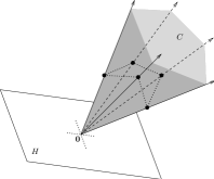
Figure 5: A pointed polyhedral cone with five basis vectors

Definition 5.5 (Basis).

Let $S$ be any set of vectors in $\R^{d}$. By a basis for $S$, we mean a subset of vectors $B\subset S$ for which

1. every vector of $S$ can be expressed as a non-negative linear combination of vectors in $B$;

2. if any vector is removed from $B$ then property (i) no longer holds.

It is straightforward to see that we can replace (ii) with the equivalent property

• no vector in $B$ can be expressed as a non-negative linear combination of the others.

Although our definition of a basis is designed with polyhedral cones in mind, it is deliberately broad; this is because we will need to apply it not only to polyhedral cones but also to non-convex sets, such as the semi-admissible parts to be defined shortly. Note that for general sets $S$, property (i) does not work in reverse—there might well be non-negative linear combinations of vectors in $B$ that are not elements of the set $S$.

For a pointed polyhedral cone $C$, the vectors in a basis correspond to the edges of the cone; these edges are also known as extremal rays of $C$. Figure 5 illustrates a pointed polyhedral cone $C$ with a supporting hyperplane $H$ as described by Definition 5.4; the five points marked in black together form a basis for $C$. The basis for a pointed polyhedral cone is essentially unique and can be used to reconstruct the cone, as noted by the following well known results.

Lemma 5.6.

Every polyhedral cone $C$ has a finite basis. Moreover, if $B$ and $B^{\prime}$ are both bases for a pointed polyhedral cone $C$, then there is a one-to-one correspondence between $B$ and $B^{\prime}$ that takes each vector to a positive scalar multiple of itself.

Lemma 5.7.

Let $B\subset\R^{d}$ be a finite set of vectors for which

1. no element of $B$ can be expressed as a non-negative linear combination of the others;

2. there is some hyperplane $H\subset\R^{d}$ passing through $\mathbf{0}$ for which every vector of $B$ lies strictly to the same side of $H$ (in particular, none of these vectors lie within $H$).

Then the set of all non-negative linear combinations of vectors in $B$ forms a pointed polyhedral cone with $B$ as its basis.

Some pairs of basis vectors are adjacent, in the sense that the corresponding edges of the cone are joined by two-dimensional faces. In Figure 5 above, adjacent pairs of basis vectors are marked by dotted lines. We define adjacency formally as follows.

Definition 5.8 (Adjacency).

Let $\mathbf{b}$ and $\mathbf{b}^{\prime}$ be two distinct basis vectors for a pointed polyhedral cone $C$. We define $\mathbf{b}$ and $\mathbf{b}^{\prime}$ to be adjacent if the smallest-dimensional face of $C$ containing both $\mathbf{b}$ and $\mathbf{b}^{\prime}$ has dimension two.

Bases of polyhedral cones provide a very limited form of uniqueness when taking non-negative linear combinations, as seen in the following simple lemma.

Lemma 5.9.

Let $B=\{\mathbf{b}_{1},\ldots,\mathbf{b}_{k}\}$ be a basis for a pointed polyhedral cone $C\subset\R^{d}$. If some $\mathbf{b}_{r}\in B$ can be written as a non-negative linear combination of basis vectors (that is, $\mathbf{b}_{r}=\sum\lambda_{i}\mathbf{b}_{i}$ where all $\lambda_{i}\geq 0$), then this linear combination must be the trivial $\mathbf{b}_{r}=\mathbf{b}_{r}$. That is, $\lambda_{r}=1$ and $\lambda_{i}=0$ for $i\neq r$.

Proof.

Suppose we have some non-negative linear combination $\mathbf{b}_{r}=\sum\lambda_{i}\mathbf{b}_{i}$. If $\lambda_{r}<1$ then we obtain $\mathbf{b}_{r}$ as a non-negative linear combination of the other basis vectors $\mathbf{b}_{i}$ ($i\neq r$), in violation of Definition 5.5. Therefore $\lambda_{r}\geq 1$, and we can subtract $\mathbf{b}_{r}$ to obtain $\mathbf{0}$ as a non-negative linear combination $\mathbf{0}=\sum\lambda_{i}^{\prime}\mathbf{b}_{i}$.

Since our cone is pointed, it has a supporting hyperplane $H$ for which $\mathbf{0}\in H$ but every $\mathbf{b}_{i}$ lies strictly to one side of $H$. The only way to obtain this with non-negative $\lambda_{i}^{\prime}$ is to set every $\lambda_{i}^{\prime}=0$, showing our original linear combination to be the trivial $\mathbf{b}_{r}=\mathbf{b}_{r}$. ∎

The uniqueness in Lemma 5.9 is limited in the sense that it only holds when $\mathbf{b}_{r}$ is a basis vector. In general, an arbitrary point $\mathbf{x}\in C$ might well be expressible as a non-negative linear combination of basis vectors in several different ways. Even for basis elements, it should be noted that Lemma 5.9 can fail for non-pointed cones.

An even weaker form of uniqueness exists for combinations of adjacent basis vectors, and indeed can be used to completely characterise adjacency as follows.

Lemma 5.10.

Let $B=\{\mathbf{b}_{1},\ldots,\mathbf{b}_{k}\}$ be a basis for a pointed polyhedral cone $C\subset\R^{d}$. Two distinct basis vectors $\mathbf{b}_{r},\mathbf{b}_{s}\in B$ are adjacent if and only if, whenever $\mu\mathbf{b}_{r}+\eta\mathbf{b}_{s}=\sum\lambda_{i}\mathbf{b}_{i}$ for $\mu,\eta,\lambda_{i}\geq 0$, we must have $\lambda_{i}=0$ for every $i\neq r,s$.

In other words, $\mathbf{b}_{r}$ and $\mathbf{b}_{s}$ are adjacent if and only if any non-negative linear combination of basis vectors $\mathbf{b}_{r}$ and $\mathbf{b}_{s}$ can only be expressed as a non-negative linear combination of basis vectors $\mathbf{b}_{r}$ and $\mathbf{b}_{s}$.

Proof.

To prove this we use two equivalent characterisations of faces for polyhedral cones, both of which are described by Brøndsted [2]:

1. A set $F\subseteq C$ is a face of $C$ if and only if $F=C$, $F=\emptyset$, or $F=C\cap H$ for some supporting hyperplane $H$;

2. A set $F\subseteq C$ is a face of $C$ if and only if (i) $F$ is convex, and (ii) whenever the open line segment $(\mathbf{x},\mathbf{y})$ contains a point in $F$ for some $\mathbf{x},\mathbf{y}\in C$, the entire closed line segment $[\mathbf{x},\mathbf{y}]$ lies in $F$.

We also note that every face of a polyhedral cone (and thus every supporting hyperplane above) must pass through the origin.

Suppose the basis vectors $\mathbf{b}_{r}$ and $\mathbf{b}_{s}$ are adjacent, and that $\mu\mathbf{b}_{r}+\eta\mathbf{b}_{s}=\sum\lambda_{i}\mathbf{b}_{i}$ for some $\mu,\eta,\lambda_{i}\geq 0$. Let $F$ be the smallest-dimensional face of $C$ containing both $\mathbf{b}_{r}$ and $\mathbf{b}_{s}$; since $F$ is two-dimensional, it cannot contain any other basis vector $\mathbf{b}_{i}$ for $i\neq r,s$.

Using (a) above, we can write $F=C\cap H$ for some supporting hyperplane $H$ passing through the origin. We see that $\mathbf{b}_{r}$ and $\mathbf{b}_{s}$ lie in $H$ and every other basis vector lies strictly to one side of $H$, whereupon our non-negative linear combination must have $\lambda_{i}=0$ for every $i\neq r,s$.

Suppose now that the basis vectors $\mathbf{b}_{r}$ and $\mathbf{b}_{s}$ are not adjacent. Let $G$ be the two-dimensional plane passing through $\mathbf{b}_{r}$, $\mathbf{b}_{s}$ and the origin; the non-adjacency of $\mathbf{b}_{r}$ and $\mathbf{b}_{s}$ shows that $G$ cannot be a face of $C$. Therefore, by (b) above, there are points $\mathbf{x},\mathbf{y}\in C$ for which $(\mathbf{x},\mathbf{y})$ meets $G$ but $[\mathbf{x},\mathbf{y}]\nsubseteq G$.

Let $\mathbf{z}\in(\mathbf{x},\mathbf{y})\cap G$. Because $\mathbf{z}\in G$ we can write $\mathbf{z}=\mu\mathbf{b}_{r}+\eta\mathbf{b}_{s}$ for some $\mu,\eta\geq 0$. On the other hand, we can also write $\mathbf{z}$ as a non-trivial convex combination of $\mathbf{x}$ and $\mathbf{y}$. Since $[\mathbf{x},\mathbf{y}]\nsubseteq G$ at least one of $\mathbf{x}$ and $\mathbf{y}$ cannot be expressed purely in terms of $\mathbf{b}_{r}$ and $\mathbf{b}_{s}$, and we obtain $\mathbf{z}=\mu\mathbf{b}_{r}+\eta\mathbf{b}_{s}=\sum\lambda_{i}\mathbf{b}_{i}$ where every $\lambda_{i}\geq 0$ and some $\lambda_{i}>0$ for $i\neq r,s$. ∎

There are other characterisations of adjacency, such as the algebraic and combinatorial conditions described by Fukuda and Prodon [9]. However, Lemma 5.10 will be more useful to us when we come to the proof of Algorithm 5.15.

The double description method, devised by Motzkin et al. [19] and improved upon by other authors since, is a standard algorithm for inductively converting a set of half-spaces that define a polyhedral cone into a basis for this same cone. The double description method plays an important role in the standard enumeration of normal surfaces; the reader is referred to [5] for both theoretical and practical details. Although we do not explicitly call upon the double description method here, we do rely on one of its core components, which is the following result.

Lemma 5.11.

Let $C\subset\R^{d}$ be a pointed polyhedral cone with basis $B$, and let $H$ be a half-space defined by the linear inequality $H=\{\mathbf{x}\in\R^{d}\,|\,\mathbf{x}\cdot\mathbf{h}\geq 0\}$. Then the intersection $C\cap H$ is also a pointed polyhedral cone, and we can compute a basis for $C\cap H$ as follows.

Partition the basis $B$ into sets $S_{0}=\{\mathbf{b}\in B\,|\,\mathbf{b}\cdot\mathbf{h}=0\}$, $S_{+}=\{\mathbf{b}\in B\,|\,\mathbf{b}\cdot\mathbf{h}>0\}$ and $S_{-}=\{\mathbf{b}\in B\,|\,\mathbf{b}\cdot\mathbf{h}<0\}$. Then a basis for $C\cap H$ is

$$S_{0}\cup S_{+}\cup\left\{\frac{(\mathbf{u}\cdot\mathbf{h})\mathbf{w}-(\mathbf{w}\cdot\mathbf{h})\mathbf{u}}{(\mathbf{u}\cdot\mathbf{h})-(\mathbf{w}\cdot\mathbf{h})}\,\left|\,\begin{array}[]{l}\mathbf{u}\in S_{+}\ \text{and}\ \mathbf{w}\in S_{-},\\ \text{$\mathbf{u},\mathbf{w}$ are adjacent basis vectors of $C$}\end{array}\right.\right\}.$$

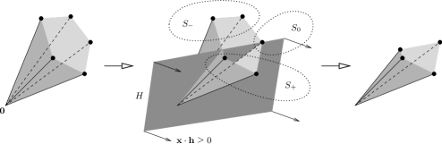
Figure 6: Intersecting a pointed polyhedral cone with a new half-space

This procedure is illustrated in Figure 6. For further details on the double description method (including Lemma 5.11), the reader is referred to the excellent overview by Fukuda and Prodon [9].

When we come to proving Algorithm 5.15, we will need to work with restricted portions of polyhedral cones that satisfy the quadrilateral constraints. This motivates the following definition.

Definition 5.12 (Semi-Admissible Part).

Consider any set of vectors $S\subseteq\R^{7n}$. The semi-admissible part of $S$, denoted $\alpha(S)$, is the subset of all vectors in $S$ that satisfy the quadrilateral constraints.

We call this the semi-admissible part because we deliberately make no mention of non-negativity or the matching equations. This is essential—in Algorithm 5.15 we deal with vectors that satisfy the quadrilateral constraints but that can have negative coordinates, and in the corresponding proof we take $i$th truncations of these vectors which can break the matching equations.

It is important to note that the semi-admissible part of a polyhedral cone $C$ may well be non-convex, and so might not be a polyhedral cone in itself. Nevertheless, $\alpha(C)$ remains closed under non-negative scalar multiplication.

The following result shows that, for “sufficiently non-negative” pointed polyhedral cones $C$, bases for $C$ and bases for $\alpha(C)$ are tightly related.

Lemma 5.13.

Let $C$ be a pointed polyhedral cone in $\R^{7n}$ where, for every $\mathbf{x}\in C$, the quadrilateral coordinates of $\mathbf{x}$ are all non-negative. If $B$ is a basis for $C$, then the semi-admissible part $\alpha(B)$ forms a basis for $\alpha(C)$. Conversely, every basis for $\alpha(C)$ can be expressed in the form $\alpha(B)$ where $B$ is a basis for $C$.

Proof.

Suppose that $B=\{\mathbf{b}_{1},\ldots,\mathbf{b}_{k}\}$ is a basis for $C$.

• Since $B$ is a basis it is clear that every $\mathbf{x}\in\alpha(C)\subseteq C$ can be expressed as $\mathbf{x}=\sum\lambda_{i}\mathbf{b}_{i}$ with all $\lambda_{i}\geq 0$. Furthermore, if $\lambda_{i}>0$ for any $\mathbf{b}_{i}$ that does not satisfy the quadrilateral constraints, the non-negativity condition on $C$ ensures that $\mathbf{x}=\lambda_{i}\mathbf{b}_{i}+\ldots$ cannot satisfy the quadrilateral constraints either. Thus $\mathbf{x}=\sum\lambda_{i}\mathbf{b}_{i}$ is actually a non-negative linear combination of vectors in $\alpha(B)$.

• Since no element of $B$ can be expressed as a non-negative linear combination of the others, the same must be true of $\alpha(B)\subseteq B$.

It follows by Definition 5.5 that $\alpha(B)$ is a basis for $\alpha(C)$.

Conversely, let $B^{\prime}$ be a basis for $\alpha(C)$, and let $B=\{\mathbf{b}_{1},\ldots,\mathbf{b}_{k}\}$ be some basis for $C$. For each $\mathbf{b}_{i}\in\alpha(B)$, we modify $B$ as follows.

• Since $B^{\prime}$ is a basis for $\alpha(C)$, we can express $\mathbf{b}_{i}$ as a non-negative linear combination of elements of $B^{\prime}$; we mark this linear combination ($\star$) for later reference. Because $B$ is a basis for $C$, we can expand ($\star$) to a non-negative linear combination of elements of $B$. Thus we obtain $\mathbf{b}_{i}=\sum\lambda_{j}\mathbf{b}_{j}$ for $\lambda_{j}\geq 0$.

  However, Lemma 5.9 shows that the only such linear combination can be $\mathbf{b}_{i}=\mathbf{b}_{i}$. Since all linear combinations are non-negative, it follows that the first linear combination ($\star$) must likewise consist only of positive multiples of $\mathbf{b}_{i}$; in particular, we must have $\mu\mathbf{b}_{i}\in B^{\prime}$ for some $\mu>0$. We now replace $\mathbf{b}_{i}$ with $\mu\mathbf{b}_{i}$ in $B$; it is clear that $B$ remains a basis for $C$.

By following this procedure for each $\mathbf{b}_{i}\in\alpha(B)$, we obtain a basis $B$ for $C$ that satisfies $B^{\prime}\supseteq\alpha(B)$. However, from the first part of this lemma $\alpha(B)$ is also a basis for $\alpha(C)$. Therefore any additional vectors in $B^{\prime}$ would be redundant, and so we have $B^{\prime}=\alpha(B)$. ∎

We conclude our brief study of polyhedral cones with an example of a semi-admissible part and its basis that we have seen before. The following observations are all immediate consequences of the relevant definitions and Lemma 5.13.

Example 5.14.

Let $C\subset\R^{7n}$ be the set of all vectors whose entries are all non-negative and which satisfy the standard matching equations for the triangulation $\mathcal{T}$. Then $C$ is a pointed polyhedral cone, the standard projective solution space $\mathscr{S}(\mathcal{T})$ is a finite cross-section of this cone (taken along the projective hyperplane $J^{7n}$), and the vertices of the polytope $\mathscr{S}(\mathcal{T})$ form a basis for $C$. Furthermore, $\alpha(C)=\R^{7n}_{a}$ (the set of all admissible vectors in $\R^{7n}$), and the standard solution set forms a basis for $\alpha(C)$.

5.2 The Main Conversion Algorithm

We are now ready to present the quadrilateral-to-standard solution set conversion algorithm in full detail. The algorithm relies on the numbering of standard coordinate positions—here we number coordinate positions $1,2,\ldots,7n$ according to Definition 2.4, so that positions $7i+\{1,2,3,4\}$ correspond to triangular coordinates and positions $7i+\{5,6,0\}$ correspond to quadrilateral coordinates. For an arbitrary vector $\mathbf{w}\in\R^{7n}$, we use the common notation whereby $w_{i}\in\R$ denotes the coordinate of $\mathbf{w}$ in the $i$th position.

Roughly speaking, the algorithm operates as follows. Given the $m$ vertices $V_{1},\ldots,V_{m}$ of the triangulation, we inductively build lists of vectors $L_{0},L_{1},\ldots,L_{m}$. Each list $L_{r}$ generates all admissible vectors that can be formed by (i) combining vectors from the quadrilateral solution space and then (ii) adding or subtracting vertex links $\ell(V_{1}),\ldots,\ell(V_{r})$. In particular, the initial list $L_{0}$ is the quadrilateral solution set, and (after appropriate scaling) the final list $L_{m}$ becomes the standard solution set.

Each inductive step that transforms $L_{r}$ into $L_{r+1}$ is based on the double description method, though complications arise because we do not have access to the full facet structures of the underlying polyhedral cones. As we construct each list $L_{r}$ we essentially ignore all triangular coordinates around the subsequent vertices $V_{r+1},\ldots,V_{m}$, though we do maintain the standard matching equations at all times. This selective ignorance is expressed in the proof through the truncation function $\tau_{r}$, and is resolved in the algorithm itself by taking the partial canonical part $\kappa_{v}^{(r)}$ when the need arises.

Algorithm 5.15.

Suppose we are given the quadrilateral solution set for the triangulation $\mathcal{T}$, and that this quadrilateral solution set consists of the $k$ vectors $\mathbf{q}_{1},\ldots,\mathbf{q}_{k}\in\R^{3n}$. Then the following algorithm computes the standard solution set for $\mathcal{T}$.

Let the vertices of $\mathcal{T}$ be $V_{1},\ldots,V_{m}$. We construct lists of vectors $L_{0},L_{1},\ldots,L_{m}\subset\R^{7n}$ as follows.

1. Fill the list $L_{0}$ with the canonical extensions $\varepsilon(\mathbf{q}_{1}),\ldots,\varepsilon(\mathbf{q}_{k})\in\R^{7n}$, using Algorithm 3.12 to perform the computations.

2. Create a set of coordinate positions $C\subseteq\{1,2,\ldots,7n\}$ and initialise this to the set of all quadrilateral coordinate positions, so that

   $$C=\{5,6,7,\ 12,13,14,\ \ldots,\ 7n-2,7n-1,7n\}.$$

   This set will grow as the algorithm runs, eventually expanding to all of $\{1,2,\ldots,7n\}$.

3. For each $r=1,2,\ldots,m$, fill the list $L_{r}$ as follows.

   1. For each vector $\mathbf{x}\in L_{r-1}$, insert the partial canonical part $\kappa_{v}^{(r)}(\mathbf{x})$ into $L_{r}$.

   2. Insert the negative vertex link $-\ell(V_{r})$ into $L_{r}$.

   3. Let $T_{r}\subset\{1,2,\ldots,7n\}$ be the set of all coordinate positions corresponding to triangular disc types in the vertex link $\ell(V_{r})$; that is, $T_{r}=\{p\,|\,\ell(V_{r})_{p}\neq 0\}$. For each position $p\in T_{r}$, perform the following steps.

      1. Partition the list $L_{r}$ into three lists $S_{0}$, $S_{+}$ and $S_{-}$ according to the sign of the $p$th coordinate. Specifically, let $S_{0}=\{\mathbf{x}\in L_{r}\,|\,x_{p}=0\}$, $S_{+}=\{\mathbf{x}\in L_{r}\,|\,x_{p}>0\}$ and $S_{-}=\{\mathbf{x}\in L_{r}\,|\,x_{p}<0\}$.

      2. Create a new temporary list $L^{\prime}=S_{0}\cup S_{+}$.

      3. Run through all pairs of vectors $\mathbf{u}\in S_{+}$ and $\mathbf{w}\in S_{-}$ that satisfy both of the following conditions:

         • $\mathbf{u}$ and $\mathbf{w}$ together satisfy the quadrilateral constraints. That is, for each tetrahedron $\Delta_{i}$ of $\mathcal{T}$, at least two of the three quadrilateral coordinates for $\Delta_{i}$ are zero in both $\mathbf{u}$ and $\mathbf{w}$ simultaneously.

         • There is no vector $\mathbf{z}\in L_{r}$ other than $\mathbf{u}$ and $\mathbf{w}$ for which, whenever a coordinate position $i\in C$ satisfies both $u_{i}=0$ and $w_{i}=0$, then $z_{i}=0$ also.

         For each such pair, insert the vector $(u_{p}\mathbf{w}-w_{p}\mathbf{u})/(u_{p}-w_{p})$ into the temporary list $L^{\prime}$. Note that this vector is the point where the line joining $\mathbf{u}$ and $\mathbf{w}$ meets the hyperplane $\{\mathbf{x}\in\R^{7n}\,|\,x_{p}=0\}$.

      4. Empty out the list $L_{r}$ and refill it with the vectors in $L^{\prime}$, and insert the coordinate position $p$ into the set $C$.

   4. Finish the list by inserting the positive vertex link $\ell(V_{r})$ into $L_{r}$.

Suppose that the very last list $L_{m}$ consists of the $k^{\prime}$ vectors $\mathbf{v}_{1},\ldots,\mathbf{v}_{k^{\prime}}\in\R^{7n}$. Then the standard solution set for $\mathcal{T}$ consists of the $k^{\prime}$ projective images $\overline{\mathbf{v}_{1}},\ldots,\overline{\mathbf{v}_{k^{\prime}}}$.

Before we embark on a proof that this algorithm is correct, there are a few points worth noting.

• Unlike the previous algorithms in this paper, the statement of Algorithm 5.15 does not include a time complexity. This is because the algorithm can grow exponentially slow with respect to the size of the input.

  For examples of this exponential growth the reader is referred to [6], which describes the solution sets for the $n$–tetrahedron twisted layered loop, a highly symmetric triangulation of the quotient space $S^{3}/Q_{4n}$. In these examples the quadrilateral solution set has size $\Theta(n)$, whereas the standard solution set has size $\Theta(\phi^{n})$ for $\phi=(1+\sqrt{5})/2$. Thus the size of the output is exponential in the size of the input, and so the running time of any conversion algorithm must be at least this bad.

  On the other hand, it is possible—and indeed quite plausible—that the running time of Algorithm 5.15 is polynomial in the size of the output. For further discussion, see Conjecture 5.16 later in this section.

• Step 3(c) bears a resemblance to the double description method of Motzkin et al. [19]. As discussed earlier, this is no accident—in a sense, within each iteration of step 3 we create a new pointed polyhedral cone and then enumerate its admissible extreme rays. The differences appear in the processing of pairs $\mathbf{u}\in S_{+}$ and $\mathbf{w}\in S_{-}$, where we deviate from the usual double description method in the constraints on $\mathbf{u}$ and $\mathbf{w}$.

• As presented, Algorithm 5.15 requires exact arithmetic on rational numbers, which may be undesirable in practice for reasons of performance or implementation. We can avoid this by observing that throughout steps 1–3 we can replace any vector $\mathbf{x}$ with any multiple $\lambda\mathbf{x}$ ($\lambda>0$) without changing the final solution set. This means that we can work entirely within the integers by rescaling vectors appropriately.

Proof of Algorithm 5.15.

This is a lengthy proof, consisting of two nested inductions corresponding to the two nested loops of steps 3 and 3(c). We therefore split this proof into six parts: I–III to establish the outer induction, and IV–VI to establish the inner induction. The road map for parts I–III is given below. Because the inner induction sits within part II, we delay the road map for parts IV–VI until then.

Our outer induction proves a statement about the finished lists $L_{0},\ldots,L_{m}$. In order to make this statement, we define the space $\mathscr{A}_{r}$ for each $r=0,\ldots,m$ to be

(1) $$\mathscr{A}_{r}\ =\ \left\{\left.\mathbf{x}=\sum_{i=1}^{k}\lambda_{i}\varepsilon(\mathbf{q}_{i})+\sum_{j=1}^{r}\mu_{j}\ell(V_{j})\ \right|\ \begin{array}[]{l}\lambda_{i}\geq 0\ \forall i\in 1..k,\\ x_{p}\geq 0\ \forall p\in 1..7n\end{array}\right\}.$$

That is, $\mathscr{A}_{r}$ consists of all non-negative vectors in $\R^{7n}$ that can be expressed as (i) a non-negative linear combination of the original $k$ vectors from the quadrilateral solution space, plus (ii) arbitrary positive or negative multiples of the first $r$ vertex links. Our key inductive claim relates the space $\mathscr{A}_{r}$ to the list $L_{r}$ as follows:

Claim: Once the list $L_{r}$ is fully constructed, it consists only of admissible vectors. Furthermore, the truncation $\tau_{r}(L_{r})$ is a basis for the semi-admissible part $\alpha(\tau_{r}(\mathscr{A}_{r}))$.

($\star$)

Our outer induction now proceeds according to the following plan.

Road map for parts I–III:

1. Show that ($\star$) is true for $r=0$;

2. Show that if ($\star$) is true for $r=i-1$ where $i>0$ then ($\star$) is also true for $r=i$;

3. Show that if ($\star$) is true for $r=m$ then Algorithm 5.15 is correct.

Because part II is significantly more complex than the others (in particular, it contains the inner induction), we shall subvert the natural order of things and deal with parts I and III first.

— Part I —

We begin with part I, where we must prove ($\star$) for $r=0$. Note that $\mathscr{A}_{0}$ can be written more simply as

$$\mathscr{A}_{0}\ =\ \left\{\left.\mathbf{x}=\sum_{i=1}^{k}\lambda_{i}\varepsilon(\mathbf{q}_{i})\ \right|\ \begin{array}[]{l}\lambda_{i}\geq 0\ \forall i\in 1..k,\\ x_{p}\geq 0\ \forall p\in 1..7n\end{array}\right\}.$$

Furthermore, because each $\varepsilon(\mathbf{q}_{i})$ is admissible the constraints $x_{p}\geq 0$ are redundant, and so $\mathscr{A}_{0}$ is merely the set of all non-negative linear combinations of $\varepsilon(\mathbf{q}_{1}),\ldots,\varepsilon(\mathbf{q}_{k})$. Because truncation is linear, $\tau_{0}(\mathscr{A}_{0})$ is likewise the set of all non-negative linear combinations of $\tau_{0}(\varepsilon(\mathbf{q}_{1})),\ldots,\tau_{0}(\varepsilon(\mathbf{q}_{k}))$. Noting that neither $\tau_{0}$ nor $\varepsilon$ affects quadrilateral coordinates, we can make the following observations:

• Suppose that some $\tau_{0}(\varepsilon(\mathbf{q}_{i}))\in\R^{7n}$ could be expressed as a linear combination of the others. Restricting our attention to quadrilateral coordinates would therefore give some $\mathbf{q}_{i}\in\R^{3n}$ as a linear combination of the others, in violation of Lemma 4.1.

• Since the vectors $\tau_{0}(\varepsilon(\mathbf{q}_{i}))$ are all non-zero vectors with non-negative coordinates, they all lie to the same side of the hyperplane $\sum x_{p}=0$.

It follows from Lemma 5.7 that $\tau_{0}(\mathscr{A}_{0})$ is a pointed polyhedral cone with $\tau_{0}(L_{0})$ as its basis. Moreover, since each $\mathbf{q}_{i}$ satisfies the quadrilateral constraints we have $\alpha(\tau_{0}(L_{0}))=\tau_{0}(L_{0})$, and so by Lemma 5.13 $\tau_{0}(L_{0})$ is a basis for $\alpha(\tau_{0}(\mathscr{A}_{0}))$ also. Finally, it is clear from construction that every vector in $L_{0}$ is admissible.

— Part III —

We now jump straight to part III, where we can ignore truncations entirely because $\tau_{m}$ is the identity map. We assume therefore that $L_{m}$ is a basis for $\alpha(\mathscr{A}_{m})$, and our task is to prove from this that the projective images of the vectors in $L_{m}$ together form the standard solution set for $\mathcal{T}$.

The key observation here is that the semi-admissible part $\alpha(\mathscr{A}_{m})$ is simply $\R^{7n}_{a}$, the set of all admissible vectors in standard coordinates. To see this:

• Every vector in $\alpha(\mathscr{A}_{m})$ has non-negative coordinates by definition of $\mathscr{A}_{m}$, and satisfies the quadrilateral constraints by definition of $\alpha$. Moreover, since every $\varepsilon(\mathbf{q}_{i})$ and $\ell(V_{j})$ satisfies the standard matching equations, so does every vector in $\alpha(\mathscr{A}_{m})$. Thus $\alpha(\mathscr{A}_{m})\subseteq\R^{7n}_{a}$.

• Let $\mathbf{x}\in\R^{7n}_{a}$. By Definition 2.11, the quadrilateral projection $\pi(\mathbf{x})$ can be expressed as a non-negative combination of vertices of the quadrilateral projective solution space $\mathscr{Q}(\mathcal{T})$. More specifically, $\pi(\mathbf{x})$ can be expressed as a non-negative combination of admissible vertices of $\mathscr{Q}(\mathcal{T})$, since otherwise $\pi(\mathbf{x})$ would not satisfy the quadrilateral constraints. Therefore $\pi(\mathbf{x})=\sum\lambda_{i}\mathbf{q}_{i}$ for some $\lambda_{i}\geq 0$.

  By chasing maps around the commutative diagram in Lemma 3.11 and recalling that $\pi$ is linear and $\varepsilon$ preserves scalar multiplication, we subsequently derive the equation $\kappa_{v}(\mathbf{x})=\kappa_{v}\left(\sum\lambda_{i}\varepsilon(\mathbf{q}_{i})\right)$. That is, $\mathbf{x}$ is a non-negative linear combination of $\varepsilon(\mathbf{q}_{i})$ plus some arbitrary linear combination of vertex links. Hence $\mathbf{x}\in\alpha(\mathscr{A}_{m})$, and we have $\R^{7n}_{a}\subseteq\alpha(\mathscr{A}_{m})$.

From here part III is straightforward. We know that $L_{m}$ is a basis for $\R^{7n}_{a}=\alpha(\mathscr{A}_{m})$, and from Example 5.14 we know that the standard solution set is a basis for $\R^{7n}_{a}$ also. Expressing $\R^{7n}_{a}$ as the semi-admissible part of a pointed polyhedral cone (Example 5.14 again), we can combine Lemmata 5.6 and 5.13 to show that the basis for $\alpha(\mathscr{A}_{m})$ is unique up to scalar multiplication. It follows that once we take projective images, the list $L_{m}$ and the standard solution set are identical.

— Part II —

All that remains is part II, the inductive step. Suppose we are constructing the list $L_{r}$ for some $r>0$. Our outer inductive hypothesis is that the list $L_{r-1}$ consists only of admissible vectors and that $\tau_{r-1}(L_{r-1})$ is a basis for $\alpha(\tau_{r-1}(\mathscr{A}_{r-1}))$. Our task is to prove that, once the list $L_{r}$ is complete, it too consists only of admissible vectors with the truncation $\tau_{r}(L_{r})$ forming a basis for $\alpha(\tau_{r}(\mathscr{A}_{r}))$.

To show this, we must dig into the construction of the list $L_{r}$ and perform a new inner induction over the constructive loop in step 3(c) of the algorithm. Suppose the list $L_{r-1}$ consists of the vectors $\mathbf{a}_{1},\ldots,\mathbf{a}_{t}$. For every set of coordinate positions $P$, we define a new space

(2) $$\mathscr{B}_{P}\ =\ \left\{\mathbf{x}=\sum_{i=1}^{t}\lambda_{i}\kappa_{v}^{(r)}(\mathbf{a}_{i})-\mu_{r}\ell(V_{r})\ \left|\ \begin{array}[]{l}\lambda_{i}\geq 0\ \forall i\in 1..t,\\ \mu_{r}\geq 0,\\ x_{p}\geq 0\ \forall p\in P\end{array}\right.\right\}.$$

Essentially, $\mathscr{B}_{P}$ is constructed by taking non-negative linear combinations of (i) the $r$th partial canonical parts of vectors in $L_{r-1}$, and (ii) the negative vertex link $-\ell(V_{r})$. Note that we relax our insistence on non-negative coordinates—vectors in $\mathscr{B}_{P}$ may include negative coordinates, as long as these only occur at coordinate positions outside the set $P$.

Our inner inductive claim is the following. It should be read as a loop invariant that applies before and after each position $p\in T_{r}$ is processed in step 3(c) of Algorithm 5.15.

Claim: Every vector $\mathbf{x}$ in the partially-constructed list $L_{r}$ satisfies both the standard matching equations and the quadrilateral constraints, and has at least one coordinate position $p\in T_{r}$ for which $x_{p}\leq 0$. Furthermore, the truncation $\tau_{r}(\mathscr{B}_{C})$ is a pointed polyhedral cone, and the truncation $\tau_{r}(L_{r})$ forms a basis for the semi-admissible part $\alpha(\tau_{r}(\mathscr{B}_{C}))$.

($\dagger$)

Note that both the list $L_{r}$ and the set $C$ continue to change as step 3(c) iterates through each position $p\in T_{r}$. Our claim is that they both change together in a way that maintains the truth of ($\dagger$).

The remainder of this proof proceeds according to the following plan. Once again, the context for this plan is that we are currently constructing the list $L_{r}$ in the $r$th iteration of step 3 of the algorithm.

Road map for parts IV–VI:

1. Show that ($\dagger$) is true when we first reach step 3(c);

2. Show that, when processing some $p\in T_{r}$ in step 3(c), if ($\dagger$) is true before running step 3(c)(i) then ($\dagger$) is still true after running step 3(c)(iv);

3. Show that, if ($\dagger$) is true after the loop in step 3(c) finishes, then ($\star$) is true at the end of step 3(d).

In other words, parts IV and V constitute an inner induction to establish the correctness of the invariant ($\dagger$) throughout the construction of the list $L_{r}$. Part VI then uses this invariant to prove the outer inductive claim ($\star$), concluding part II and the proof of Algorithm 5.15.

Throughout parts IV–VI we continue to assume the outer inductive hypothesis; that is, that $L_{r-1}$ consists of the admissible vectors $\mathbf{a}_{1},\ldots,\mathbf{a}_{t}$, and that the truncation $\tau_{r-1}(L_{r-1})$ forms a basis for $\alpha(\tau_{r-1}(\mathscr{A}_{r-1}))$.

— Part IV —

We begin our inner induction with part IV, at the point where we first reach step 3(c). At this point in the algorithm, the relevant variables take the following values:

• $L_{r}$ consists of $\kappa_{v}^{(r)}(\mathbf{a}_{1})$, …, $\kappa_{v}^{(r)}(\mathbf{a}_{t})$ and the negative vertex link $-\ell(V_{r})$;

• $C$ consists of all quadrilateral coordinate positions, as well as the triangular coordinate positions in sets $T_{1},\ldots,T_{r-1}$.

Our task is to show that the claim ($\dagger$) holds true for these values of $L_{r}$ and $C$.

It is clear from construction that every $\mathbf{x}\in L_{r}$ has at least one coordinate position $p\in T_{r}$ for which $x_{p}\leq 0$. Moreover, since the outer inductive hypothesis shows that every $\mathbf{a}_{i}$ is admissible, we can see that (i) every $\mathbf{x}\in L_{r}$ satisfies both the standard matching equations and the quadrilateral constraints, and that (ii) the only coordinates in any $\mathbf{x}\in L_{r}$ that might be negative are those in positions $p\in T_{r}$. Noting that $T_{r}\cap C=\emptyset$, the constraint $x_{p}\geq 0\ \forall p\in C$ in equation (2) is therefore redundant in this case, and we simply have

(3) $$\mathscr{B}_{C}\ =\ \left\{\left.\mathbf{x}=\sum_{i=1}^{t}\lambda_{i}\kappa_{v}^{(r)}(\mathbf{a}_{i})-\mu_{r}\ell(V_{r})\ \right|\ \begin{array}[]{l}\lambda_{i}\geq 0\ \forall i\in 1..t,\\ \mu_{r}\geq 0\end{array}\right\}.$$

It remains to show that $\tau_{r}(\mathscr{B}_{C})$ is a pointed polyhedral cone, and that $\tau_{r}(L_{r})$ forms a basis for $\alpha(\tau_{r}(\mathscr{B}_{C}))$.

From (3) it is clear that $\mathscr{B}_{C}$ is the set of all non-negative linear combinations of vectors in $L_{r}$, and thus $\tau_{r}(\mathscr{B}_{C})$ is the set of all non-negative linear combinations of vectors in $\tau_{r}(L_{r})$. We now focus on establishing the conditions of Lemma 5.7 for the list $\tau_{r}(L_{r})$.

1. Suppose that some vector in $\tau_{r}(L_{r})$ can be written as a non-negative linear combination of the other vectors in $\tau_{r}(L_{r})$. Taking the linear map $\tau_{r-1}$ and recalling that $\tau_{r-1}\circ\tau_{r}=\tau_{r-1}$, it follows that the corresponding vector in $\tau_{r-1}(L_{r})$ can be written as the same non-negative linear combination of the other vectors in $\tau_{r-1}(L_{r})$.

   For each $\kappa_{v}^{(r)}(\mathbf{a}_{i})\in L_{r}$ we have $\tau_{r-1}(\kappa_{v}^{(r)}(\mathbf{a}_{i}))=\tau_{r-1}(\mathbf{a}_{i})$, and for $-\ell(V_{r})\in L_{r}$ we have $\tau_{r-1}(-\ell(V_{r}))=\mathbf{0}$. Thus $\tau_{r-1}(L_{r})$ consists of the basis $\tau_{r-1}(L_{r-1})$ combined with the zero vector, and so the only possible non-negative linear combination in $\tau_{r-1}(L_{r})$ is the trivial combination $\tau_{r-1}(-\ell(V_{r}))=\mathbf{0}$. It follows that our original non-negative linear combination in $\tau_{r}(L_{r})$ must have been $\tau_{r}(-\ell(V_{r}))=\mathbf{0}$, a contradiction.

2. We aim now to construct a hyperplane $H\subset\R^{7n}$ for which every vector in $\tau_{r}(L_{r})$ lies strictly to the same side of $H$. To do this, we define the temporary vector $\mathbf{u}=\tau_{r-1}(\mathbf{1})$. That is, $\mathbf{u}$ contains 1 in all quadrilateral coordinate positions as well as the triangle positions $p\in T_{1}\cup\ldots\cup T_{r-1}$, and contains 0 in the remaining triangle positions $p\in T_{r}\cup\ldots\cup T_{m}$. Recall also that the vertex link $\ell(V_{r})$ contains 1 in all triangle positions $p\in T_{r}$, and contains 0 in all other triangle and quadrilateral positions.

   Define the constants

   $$g=\min_{i=1}^{t}\left\{\mathbf{u}\cdot\tau_{r}(\kappa_{v}^{(r)}(\mathbf{a}_{i}))\right\}\quad\text{and}\quad h=\max_{i=1}^{t}\left\{\ell(V_{r})\cdot\tau_{r}(\kappa_{v}^{(r)}(\mathbf{a}_{i}))\right\}.$$

   Since $\tau_{r-1}(L_{r-1})$ is a basis of non-negative vectors and $\mathbf{u}\cdot\tau_{r}(\kappa_{v}^{(r)}(\mathbf{a}_{i}))=\mathbf{u}\cdot\tau_{r-1}(\mathbf{a}_{i})$, it is clear that $g>0$. Furthermore, from the definition of $\kappa_{v}^{(r)}$ and the fact that $\ell(V_{r})\cdot\tau_{r}(\kappa_{v}^{(r)}(\mathbf{a}_{i}))=\ell(V_{r})\cdot\kappa_{v}^{(r)}(\mathbf{a}_{i})$ it is clear that $h\geq 0$.

   Let $H$ be the hyperplane $\{\mathbf{x}\in\R^{7n}\,|\,(h+1)\mathbf{u}\cdot\mathbf{x}=g\,\ell(V_{r})\cdot\mathbf{x}\}$. We show now that every element of $\tau_{r}(L_{r})$ lies strictly to the same side of $H$. By definition of $g$ and $h$, if $\mathbf{x}=\tau_{r}(\kappa_{v}^{(r)}(\mathbf{a}_{i}))\in\tau_{r}(L_{r})$ then we have $(h+1)\mathbf{u}\cdot\mathbf{x}\geq(h+1)g>g\,h\geq g\,\ell(V_{r})\cdot\mathbf{x}$. Finally, if $\mathbf{x}=\tau_{r}(-\ell(V_{r}))\in\tau_{r}(L_{r})$ then this simplifies to $\mathbf{x}=-\ell(V_{r})$, and so $(h+1)\mathbf{u}\cdot\mathbf{x}=0>g\,\ell(V_{r})\cdot\mathbf{x}$. Therefore $H$ is the hyperplane that we require.

It follows from Lemma 5.7 that $\tau_{r}(\mathscr{B}_{C})$ is a pointed polyhedral cone with $\tau_{r}(L_{r})$ as its basis. Finally, since every $\mathbf{a}_{i}$ is admissible it is clear that every vector of $\tau_{r}(L_{r})$ satisfies the quadrilateral constraints; thus $\alpha(\tau_{r}(L_{r}))=\tau_{r}(L_{r})$, and Lemma 5.13 shows that $\tau_{r}(L_{r})$ is a basis for $\alpha(\tau_{r}(\mathscr{B}_{C}))$ also.

— Part V —

We come now to part V, the main inductive step for the inner induction. Here we assume that ($\dagger$) holds before running step 3(c)(i); our task is to show that ($\dagger$) still holds after running step 3(c)(iv).

Throughout this part, we assume that we are building the list $L_{r}$, and that we are currently processing some coordinate position $p\in T_{r}$. We use the following notation:

• $L_{r}$ and $C$ denote the initial states of these variables, before step 3(c)(i).

• $S_{0}$, $S_{+}$ and $S_{-}$ are as defined in Algorithm 5.15; that is, $S_{0}=\{\mathbf{x}\in L_{r}\,|\,x_{p}=0\}$, $S_{+}=\{\mathbf{x}\in L_{r}\,|\,x_{p}>0\}$ and $S_{-}=\{\mathbf{x}\in L_{r}\,|\,x_{p}<0\}$.

• $L^{\prime}$ denotes the final state of the list after step 3(c)(iv). In other words,

(4) $$L^{\prime}=S_{0}\cup S_{+}\cup\left\{\frac{u_{p}\mathbf{w}-w_{p}\mathbf{u}}{u_{p}-w_{p}}\,\left|\,\begin{array}[]{l}\mathbf{u}\in S_{+}\ \text{and}\ \mathbf{w}\in S_{-},\\ \text{$\mathbf{u},\mathbf{w}$ together satisfy the quad.~{}constraints,}\\ \nexists\mathbf{z}\in L_{r}\backslash\{\mathbf{u},\mathbf{w}\}\ \text{for which}\\ \quad\left(i\in C\cup\{p\}\ \text{and}\ u_{i}=w_{i}=0\right)\Rightarrow z_{i}=0\end{array}\right.\right\}.$$

In addition, we note that the final state of the set $C$ is simply $C\cup\{p\}$. We can therefore assume claim ($\dagger$) exactly as written, and our task is to prove the following:

1. Every $\mathbf{x}\in L^{\prime}$ satisfies both the standard matching equations and the quadrilateral constraints, and has at least one coordinate position $p^{\prime}\in T_{r}$ for which $x_{p^{\prime}}\leq 0$;

2. The truncation $\tau_{r}(\mathscr{B}_{C\cup\{p\}})$ is a pointed polyhedral cone;

3. The truncation $\tau_{r}(L^{\prime})$ forms a basis for $\alpha(\tau_{r}(\mathscr{B}_{C\cup\{p\}}))$.

Claim (a) is straightforward; these properties are already known to be true for all vectors in $S_{0},S_{+},S_{-}\subseteq L_{r}$, and it is clear by construction that they also hold for vectors new to $L^{\prime}$. In particular, $x_{p}=0$ for each new vector $\mathbf{x}=(u_{p}\mathbf{w}-w_{p}\mathbf{u})/(u_{p}-w_{p})$. Claim (b) is also straightforward, since equation (2) shows that $\tau_{r}(\mathscr{B}_{C\cup\{p\}})$ is the intersection of the pointed polyhedral cone $\tau_{r}(\mathscr{B}_{C})$ with the half-space $x_{p}\geq 0$. We therefore focus our efforts on proving (c), that is, that $\tau_{r}(L^{\prime})$ forms a basis for $\alpha(\tau_{r}(\mathscr{B}_{C\cup\{p\}}))$.

We know from ($\dagger$) that $L_{r}$ forms a basis for $\alpha(\tau_{r}(\mathscr{B}_{C}))$, where $\tau_{r}(\mathscr{B}_{C})$ is a pointed polyhedral cone. From Lemma 5.13, there is a basis $M$ for $\tau_{r}(\mathscr{B}_{C})$ for which $L_{r}=\alpha(M)$. As noted earlier, the final polyhedral cone $\tau_{r}(\mathscr{B}_{C\cup\{p\}})$ is simply $\tau_{r}(\mathscr{B}_{C})$ intersected with the half-space $x_{p}\geq 0$; our plan is to use this fact to convert $M$ into a basis for $\tau_{r}(\mathscr{B}_{C\cup\{p\}})$ and then a basis for $\alpha(\tau_{r}(\mathscr{B}_{C\cup\{p\}}))$, which we will see is simply the final list $L^{\prime}$.

To convert $M$ into a basis for $\tau_{r}(\mathscr{B}_{C\cup\{p\}})$, we call upon the regular double description method. Just as $M$ is a superset of $L_{r}$, we define the supersets $M_{0}=\{\mathbf{m}\in M\,|\,m_{p}=0\}\supseteq S_{0}$, $M_{+}=\{\mathbf{m}\in M\,|\,m_{p}>0\}\supseteq S_{+}$ and $M_{-}=\{\mathbf{m}\in M\,|\,m_{p}<0\}\supseteq S_{-}$. Lemma 5.11 then shows that the following is a basis for $\tau_{r}(\mathscr{B}_{C\cup\{p\}})=\tau_{r}(\mathscr{B}_{C})\cap\{\mathbf{x}\,|\,x_{p}\geq 0\}$:

$$M^{\prime}=M_{0}\cup M_{+}\cup\left\{\frac{u_{p}\mathbf{w}-w_{p}\mathbf{u}}{u_{p}-w_{p}}\,\left|\,\begin{array}[]{l}\mathbf{u}\in M_{+}\ \text{and}\ \mathbf{w}\in M_{-},\\ \text{$\mathbf{u},\mathbf{w}$ are adjacent basis vectors in $\tau_{r}(\mathscr{B}_{C})$}\end{array}\right.\right\}.$$

Using Lemma 5.13 and the observation that $u_{p}>0>w_{p}$, a corresponding basis for the semi-admissible part $\alpha(\tau_{r}(\mathscr{B}_{C\cup\{p\}}))$ is

$$\alpha(M^{\prime})=S_{0}\cup S_{+}\cup\left\{\frac{u_{p}\mathbf{w}-w_{p}\mathbf{u}}{u_{p}-w_{p}}\,\left|\,\begin{array}[]{l}\mathbf{u}\in S_{+}\ \text{and}\ \mathbf{w}\in S_{-},\\ \text{$\mathbf{u},\mathbf{w}$ together satisfy the quad.~{}constraints,}\\ \text{$\mathbf{u},\mathbf{w}$ are adjacent basis vectors in $\tau_{r}(\mathscr{B}_{C})$}\end{array}\right.\right\}.$$

Consider the following claim, which we will prove shortly.

Claim: Suppose $\mathbf{u}$ and $\mathbf{w}$ are basis vectors for $\tau_{r}(\mathscr{B}_{C})$ that together satisfy the quadrilateral constraints. Then $\mathbf{u}$ and $\mathbf{w}$ are adjacent if and only if there is no $\mathbf{z}\in M\backslash\{\mathbf{u},\mathbf{w}\}$ for which, whenever $i\in C$ and $u_{i}=w_{i}=0$, we must have $z_{i}=0$.

(※)

If this is true, then our basis for $\alpha(\tau_{r}(\mathscr{B}_{C\cup\{p\}}))$ can be rewritten as

$$\alpha(M^{\prime})=S_{0}\cup S_{+}\cup\left\{\frac{u_{p}\mathbf{w}-w_{p}\mathbf{u}}{u_{p}-w_{p}}\,\left|\,\begin{array}[]{l}\mathbf{u}\in S_{+}\ \text{and}\ \mathbf{w}\in S_{-},\\ \text{$\mathbf{u},\mathbf{w}$ together satisfy the quad.~{}constraints,}\\ \nexists\mathbf{z}\in M\backslash\{\mathbf{u},\mathbf{w}\}\ \text{for which}\\ \quad\left(i\in C\ \text{and}\ u_{i}=w_{i}=0\right)\Rightarrow z_{i}=0\end{array}\right.\right\}.$$

Because $C$ contains all quadrilateral positions, we can change $\mathbf{z}\in M\backslash\{\mathbf{u},\mathbf{w}\}$ in the final condition above to $\mathbf{z}\in L_{r}\backslash\{\mathbf{u},\mathbf{w}\}$. Furthermore, because $u_{p},w_{p}\neq 0$ we can change $i\in C$ in this same condition to $i\in C\cup\{p\}$. The equation then becomes identical to (4), and we see that our basis $\alpha(M^{\prime})$ is indeed the final list $L^{\prime}$.

The only thing now remaining for part V is to prove the claim (※). We do this using Lemma 5.10.

Suppose that $\mathbf{u}$ and $\mathbf{w}$ are not adjacent basis vectors in $\tau_{r}(\mathscr{B}_{C})$. By Lemma 5.10 there is some $\mathbf{x}\in\tau_{r}(\mathscr{B}_{C})$ and some coefficients $\mu,\eta,\lambda_{j}\geq 0$ for which $\mathbf{x}=\mu\mathbf{u}+\eta\mathbf{w}=\sum\lambda_{j}\mathbf{b}_{j}$, where each $\mathbf{b}_{j}$ is a basis vector for $\tau_{r}(\mathscr{B}_{C})$ and where $\lambda_{j}>0$ for some $\mathbf{b}_{j}\neq\mathbf{u},\mathbf{w}$. Because the $i$th coordinate of every basis vector is non-negative for every $i\in C$, it follows that whenever $u_{i}=w_{i}=0$ for $i\in C$ we must have $(\mathbf{b}_{j})_{i}=0$ also. Therefore $\mathbf{b}_{j}$ satisfies the conditions for $\mathbf{z}$ as specified in (※).

Suppose now that $\mathbf{u}$ and $\mathbf{w}$ are adjacent basis vectors in $\tau_{r}(\mathscr{B}_{C})$ that together satisfy the quadrilateral constraints, and that $\mathbf{z}$ is some different basis vector for which, whenever $i\in C$ and $u_{i}=w_{i}=0$, we have $z_{i}=0$ also. We show that this leads to a contradiction.

Let $\mathbf{x}=\mathbf{u}+\xi\mathbf{w}$ where $\xi>0$ is chosen so that $x_{p}<0$, and let $\mathbf{y}=\mathbf{x}-\epsilon\mathbf{z}$ for some small $\epsilon>0$. If $\mathbf{y}\in\tau_{r}(\mathscr{B}_{C})$ then we can express $\mathbf{y}=\sum\lambda_{i}\mathbf{b}_{i}$, where each $\lambda_{i}\geq 0$ and each $\mathbf{b}_{i}$ is a basis vector for $\tau_{r}(\mathscr{B}_{C})$. This gives us $\mathbf{x}=\mathbf{u}+\xi\mathbf{w}=\epsilon\mathbf{z}+\sum\lambda_{i}\mathbf{b}_{i}$, whereupon Lemma 5.10 shows that $\mathbf{u}$ and $\mathbf{w}$ cannot be adjacent, giving us the contradiction that we seek.

It remains to prove that $\mathbf{y}\in\tau_{r}(\mathscr{B}_{C})$. The condition on $\mathbf{z}$ ensures that for sufficiently small $\epsilon>0$ we have $y_{i}\geq 0$ for all $i\in C$, so all we need to show is that $\mathbf{y}$ can be expressed as a linear combination $\mathbf{y}=\sum_{i}\lambda_{i}\kappa_{v}^{(r)}(\mathbf{a}_{i})-\mu_{r}\ell(V_{r})$ for $\lambda_{i},\mu_{r}\geq 0$.

From (2) all vectors in $\mathscr{B}_{C}$ satisfy the standard matching equations. Since $\mathbf{y}$ is a linear combination of vectors in $\tau_{r}(\mathscr{B}_{C})$, it follows that $\mathbf{y}=\tau_{r}(\mathbf{y}^{\prime})$ for some $\mathbf{y}^{\prime}\in\R^{7n}$ that also satisfies the standard matching equations. Because $y_{i}\geq 0$ for all $i\in C$ we see that both $\mathbf{y}$ and $\mathbf{y}^{\prime}$ satisfy the quadrilateral constraints, and that $\mathbf{y}^{\prime}+\sum_{i=r}^{m}\zeta_{i}\ell(V_{i})$ is a non-negative vector for some coefficients $\zeta_{r},\ldots,\zeta_{m}\in\R$. Therefore $\mathbf{y}^{\prime}+\sum_{i=r}^{m}\zeta_{i}\ell(V_{i})$ is admissible.

It follows that $\pi(\mathbf{y}^{\prime}+\sum_{i=r}^{m}\zeta_{i}\ell(V_{i}))=\pi(\mathbf{y}^{\prime})\in\R^{3n}$ can be expressed as a non-negative linear combination of vectors in the quadrilateral solution set, and so from equation (1) we see that $\tau_{r-1}(\mathbf{y}^{\prime}+\sum_{i=r}^{m}\zeta_{i}\ell(V_{i}))=\tau_{r-1}(\mathbf{y}^{\prime})\in\tau_{r-1}(\mathscr{A}_{r-1})$. Using the quadrilateral constraints for $\mathbf{y}^{\prime}$ we then obtain $\tau_{r-1}(\mathbf{y}^{\prime})\in\alpha(\tau_{r-1}(\mathscr{A}_{r-1}))$, and so $\tau_{r-1}(\mathbf{y}^{\prime})=\sum_{i=1}^{t}\lambda_{i}\tau_{r-1}(\mathbf{a}_{i})$ for some $\lambda_{1},\ldots,\lambda_{t}\geq 0$.

Because $\mathbf{y^{\prime}}$ is admissible, Lemma 5.3 shows that the only error we can introduce by replacing $\tau_{r-1}$ with $\tau_{r}$ is a multiple of the vertex link $\ell(V_{r})$. Therefore $\mathbf{y}=\tau_{r}(\mathbf{y}^{\prime})=\sum_{i=1}^{t}\lambda_{i}\tau_{r}(\mathbf{a}_{i})+\mu\ell(V_{r})$ for some coefficient $\mu\in\R$. Since the partial canonical part $\kappa_{v}^{(r)}$ only adds or subtracts multiples of $\ell(V_{r})$, we can rewrite this as $\mathbf{y}=\sum_{i=1}^{t}\lambda_{i}\kappa_{v}^{(r)}(\tau_{r}(\mathbf{a}_{i}))+\mu^{\prime}\ell(V_{r})$. Finally, because we chose $\mathbf{x}$ and $\mathbf{y}$ to satisfy $y_{p}\leq x_{p}<0$ we must have $\mu^{\prime}<0$, and equation (2) shows that $\mathbf{y}\in\tau_{r}(\mathscr{B}_{C})$ as required.

— Part VI —

Moving to the final part VI, we now assume that ($\dagger$) holds at the end of step 3(c) of the algorithm; our task then is to prove that ($\star$) holds at the end of step 3(d).

At this stage of the algorithm, the set $C$ contains all positions $p\in T_{r}$ (amongst others). Consider any $\mathbf{x}\in\mathscr{B}_{C}$. We know that $\mathbf{x}$ can be expressed as a non-negative vector minus $\mu_{r}\ell(V_{r})$, but we also know that $x_{p}\geq 0$ for all $p\in C\supseteq T_{r}$. It follows that every $\mathbf{x}\in\mathscr{B}_{C}$ is a non-negative vector, and so in this case we can write $\mathscr{B}_{C}$ as

(5) $$\mathscr{B}_{C}\ =\ \left\{\mathbf{x}=\sum_{i=1}^{t}\lambda_{i}\kappa_{v}^{(r)}(\mathbf{a}_{i})-\mu_{r}\ell(V_{r})\ \left|\ \begin{array}[]{l}\lambda_{i}\geq 0\ \forall i\in 1..t,\\ \mu_{r}\geq 0,\\ x_{p}\geq 0\ \forall p\in 1..7n\end{array}\right.\right\}.$$

That is, we can replace the specific condition $x_{p}\geq 0\ \forall p\in C$ with the more general condition $x_{p}\geq 0\ \forall p\in 1..7n$.

We pick off the easy part of ($\star$) first. From ($\dagger$) we know that after step 3(c) every $\mathbf{x}\in L_{r}$ satisfies both the standard matching equations and the quadrilateral constraints, and from (5) every $\mathbf{x}\in L_{r}$ is a non-negative vector also. Thus $L_{r}$ consists only of admissible vectors, and inserting the vertex link in step 3(d) does not change this fact.

It remains to prove that $\tau_{r}(L_{r})$ forms a basis for $\alpha(\tau_{r}(\mathscr{A}_{r}))$. We do this directly through Definition 5.5.

1. At the end of step 3(c) of the algorithm, we know from ($\dagger$) that $\tau_{r}(L_{r})$ forms a basis for $\alpha(\tau_{r}(\mathscr{B}_{C}))$. It follows that $\tau_{r}(L_{r})\subseteq\alpha(\tau_{r}(\mathscr{B}_{C}))$, and that every $\mathbf{x}\in\alpha(\tau_{r}(\mathscr{B}_{C}))$ can be expressed as a non-negative linear combination of vectors in $\tau_{r}(L_{r})$. We aim to show the same for every $\mathbf{x}\in\alpha(\tau_{r}(\mathscr{A}_{r}))$ at the end of step 3(d).

   It can be seen from the definition of $\mathscr{A}_{r}$ that

   $$\mathscr{A}_{r}\ =\ \{\mathbf{x}=\mathbf{a}+\mu\ell(V_{r})\,|\,\mathbf{a}\in\mathscr{A}_{r-1}\ \text{and}\ x_{p}\geq 0\ \forall p\in 1..7n\},\ \text{and hence}$$

   $$\alpha(\tau_{r}(\mathscr{A}_{r}))\ =\ \{\mathbf{x}=\mathbf{a}+\mu\ell(V_{r})\,|\,\mathbf{a}\in\alpha(\tau_{r}(\mathscr{A}_{r-1}))\ \text{and}\ x_{p}\geq 0\ \forall p\in 1..7n\}.$$

   We now call upon the outer inductive hypothesis; in particular, the fact that $\tau_{r-1}(L_{r-1})$ is a basis for $\alpha(\tau_{r-1}(\mathscr{A}_{r-1}))$. Combining this with Lemma 5.3 to replace $\tau_{r-1}$ with $\tau_{r}$, our equation becomes

   $$\alpha(\tau_{r}(\mathscr{A}_{r}))\ =\ \alpha\left(\left\{\mathbf{x}=\sum_{i=1}^{t}\lambda_{i}\tau_{r}(\mathbf{a}_{i})+\mu\ell(V_{r})\ \left|\ \begin{array}[]{l}\lambda_{i}\geq 0\ \forall i\in 1..t,\\ x_{p}\geq 0\ \forall p\in 1..7n\end{array}\right.\right\}\right).$$

   Finally, using equation (5) and the fact that $\kappa_{v}^{(r)}$ only ever adds or subtracts copies of $\ell(V_{r})$, we obtain

   $$\alpha(\tau_{r}(\mathscr{A}_{r}))=\{\mathbf{b}+\mu\ell(V_{r})\,|\,\mathbf{b}\in\alpha(\tau_{r}(\mathscr{B}_{C}))\ \text{and}\ \mu\geq 0\}.$$

   That is, $\alpha(\tau_{r}(\mathscr{A}_{r}))$ consists of all non-negative linear combinations of (a) vectors in $\alpha(\tau_{r}(\mathscr{B}_{C}))$, and (b) the vertex link $\ell(V_{r})$. It follows from ($\dagger$) that, once we insert the vertex link into $L_{r}$ in step 3(d) of the algorithm, we know that $\tau_{r}(L_{r})\subseteq\alpha(\tau_{r}(\mathscr{A}_{r}))$ and that every $\mathbf{x}\in\alpha(\tau_{r}(\mathscr{A}_{r}))$ can be expressed as a non-negative linear combination of vectors in $\tau_{r}(L_{r})$.

2. We now show that, after step 3(d) of the algorithm, no vector in $\tau_{r}(L_{r})$ can be expressed as a non-negative linear combination of the others. Let $L_{r}^{\prime}$ be the list $L_{r}$ as it was immediately after step 3(c) (that is, without the vertex link); from ($\dagger$) we know this property is true for $\tau_{r}(L_{r}^{\prime})$. Denote the vectors in $L_{r}^{\prime}$ as $\mathbf{b}_{1},\ldots,\mathbf{b}_{q}$.

   Suppose that some vector in $\tau_{r}(L_{r})$ can be expressed as a non-negative linear combination of the others. Because the list $\tau_{r}(L_{r})$ contains only the basis elements $\tau_{r}(\mathbf{b}_{1}),\ldots,\tau_{r}(\mathbf{b}_{q})$ and the vertex link $\ell(V_{r})$, our expression must be of one of the following two types:

   • $\tau_{r}(\mathbf{b}_{i})=\sum_{j\neq i}\lambda_{j}\tau_{r}(\mathbf{b}_{j})+\mu\ell(V_{r})$ for $\lambda_{j}\geq 0$ and $\mu>0$. That is, the vertex link $\ell(V_{r})$ appears as a non-empty part of this linear combination.

     Because $\mathbf{b}_{i}$ is a non-negative vector, the clause $x_{p}\leq 0$ in ($\dagger$) implies that $\kappa_{v}(\mathbf{b}_{i})=\mathbf{b}_{i}$. However, because every $\mathbf{b}_{j}$ is also a non-negative vector, the presence of the vertex link on the right hand side above implies that

     $$\kappa_{v}\left(\sum_{j\neq i}\lambda_{j}\tau_{r}(\mathbf{b}_{j})+\mu\ell(V_{r})\right)\neq\sum_{j\neq i}\lambda_{j}\tau_{r}(\mathbf{b}_{j})+\mu\ell(V_{r}).$$

     That is, $\kappa_{v}(\mathbf{b}_{i})\neq\mathbf{b}_{i}$, giving us a contradiction.

   • $\ell(V_{r})=\sum_{j}\lambda_{j}\tau_{r}(\mathbf{b}_{j})$ for $\lambda_{j}\geq 0$. That is, the vertex link $\ell(V_{r})$ can be expressed as a non-negative linear combination of truncated vectors in $L_{r}^{\prime}$.

     Since all $\mathbf{b}_{j}$ are non-negative, every $\mathbf{b}_{j}$ that features in this linear combination must have all its quadrilateral coordinates equal to zero. Each such $\mathbf{b}_{j}$ is also admissible, whereupon Lemma 3.11 can be used to show it is a non-negative combination of vertex links. More precisely, non-negativity again shows that each corresponding $\tau_{r}(\mathbf{b}_{j})$ must be a multiple of the single vertex link $\ell(V_{r})$. However, this yields the expression $\tau_{r}(\mathbf{b}_{j})=\mu\ell(V_{r})$, which we have shown above to be impossible.

This concludes the requirements for Definition 5.5, whereupon we see that $\tau_{r}(L_{r})$ must form a basis for $\alpha(\tau_{r}(\mathscr{A}_{r}))$. Indeed, this also concludes part VI, and therefore the entire proof of Algorithm 5.15. ∎

5.3 Time Complexity and the Enumeration Algorithm

We now return to the issue of time complexity, which was raised briefly following the statement of the quadrilateral-to-standard solution set conversion algorithm (Algorithm 5.15). It has already been noted that this conversion algorithm can grow exponentially slow in the size of the input; it is also seen in [5] that the enumeration algorithms for the standard and quadrilateral solution space suffer from the same problem.

We have already discussed examples where the size of the standard solution space is exponential in $n$ (punishing the enumeration algorithm) and also exponential in the size of the quadrilateral solution space (punishing the conversion algorithm). However, this is not our worst problem. The intermediate lists that are created by these algorithms can potentially grow exponentially large with respect to both the input and the output, leading to situations where both the standard and quadrilateral solution space are very small, yet the enumeration algorithms take a very long time to run.

The root of the problem lies in the double description method, upon which the enumeration algorithms are built. Using Lemma 5.11, the double description method inductively builds a series of lists, the last of which becomes the standard or quadrilateral solution space. It is well known that the double description method can suffer from a combinatorial explosion, where the intermediate lists can grow exponentially large before shrinking back down to what might be a very small output set. See [1, 9] for discussions of how this combinatorial explosion can be tamed in general, and [5] for techniques specific to normal surface enumeration.

Because the quadrilateral-to-standard conversion algorithm incorporates aspects of the double description method, one should expect it to suffer from the same problems. However, empirical evidence suggests that it does not—in Section 6 we find that the intermediate lists in Algorithm 5.15 appear not to explode in size (never growing larger than $1\frac{1}{2}$ times the output size), and that the total running time for conversion appears to be negligible in comparison to enumeration. In light of these observations, we put forward the following proposal.

Conjecture 5.16.

The time complexity of Algorithm 5.15 is at worst polynomial in the size of the output. That is, the running time is at most a polynomial function of $n$ (the number of tetrahedra) and $k^{\prime}$ (the size of the standard solution set).

More specifically, it seems reasonable to believe based on experimental evidence that the intermediate lists for Algorithm 5.15 are at worst linear in $k^{\prime}$, from which Conjecture 5.16 would follow as an immediate consequence. A possible cause could be the highly structured ways in which the intermediate polyhedral cones $\mathscr{A}_{r}$ and $\mathscr{B}_{C}$ are formed in the proof of Algorithm 5.15.

We finish this section with the new enumeration algorithm that was promised in the introduction and again at the beginning of Section 5. Specifically, we use Algorithm 5.15 as a key component in a new algorithm for enumerating the standard solution space. As discussed in the introduction, the enumeration problem has great practical significance in normal surface theory but suffers from the feasibility problems of an exponential running time. In this context, the new algorithm below is a significant improvement—we find in Section 6 that for large cases it runs thousands and even millions of times faster than the current state-of-the-art.

This current state-of-the-art is described in [5]; essentially we begin with the double description method of Motzkin et al. [19], apply the filtering techniques of Letscher, and then incorporate a range of further improvements that exploit special properties of the normal surface enumeration problem. We refer to this modified double description method as direct enumeration.

Our new enumeration algorithm combines direct enumeration with Algorithm 5.15, and runs as follows.

Algorithm 5.17.

To compute the standard solution set for the triangulation $\mathcal{T}$, we can use the following algorithm.

1. Use direct enumeration to compute the quadrilateral solution set for $\mathcal{T}$.

2. Use Algorithm 5.15 to convert this quadrilateral solution set into the standard solution set for $\mathcal{T}$.

We expect this algorithm to perform well—although the direct enumeration in quadrilateral coordinates (step 1) remains exponentially slow, in practice it runs many orders of magnitude faster than a direct enumeration in standard coordinates [5]. Following this, the quadrilateral-to-standard conversion (step 2) is found to run extremely quickly, as discussed above.

All that remains is to test these claims in practice, which brings us to the final section of this paper.

6 Measuring Performance

To conclude this paper we measure the performance of our new algorithms through a series of practical tests. These tests involve running both old and new algorithms over 500 different triangulations, taking a variety of measurements along the way.

The triangulations chosen for these tests are the first 500 orientable triangulations from the Hodgson–Weeks closed hyperbolic census [13]; their sizes range from 9 to 25 tetrahedra. All computations were performed on a single 2.3 GHz AMD Opteron processor using the software package Regina [3, 4]. There are alternative implementations of normal surface enumeration available, notably the FXrays software by Culler and Dunfield [7]; we use Regina here because, with the improvements of [5], it is found in the author’s experience to have the greater efficiency in both time and memory for large triangulations.

Our first tests compare running times for the new enumeration algorithm in standard coordinates (Algorithm 5.17) against the old state-of-the-art (the modified double description method of [5], referred to earlier as “direct enumeration”). The following observations can be made:

• Figure 7 plots new running times directly against old running times, with one point for each of the 500 triangulations. Both axes use a log scale, since running times for both algorithms are spread out across several orders of magnitude. The diagonal lines are guides to illustrate the magnitude of the improvements.

  

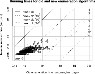
  Figure 7: Comparing the old direct enumeration against the new Algorithm 5.17

  It is immediately clear that the new algorithm is faster, and significantly so. The weakest improvement is still over $10$ times the speed, and the strongest is over $2\,000\,000$ times. Roughly speaking, the largest cases experience the greatest improvements (which is what we hope for). Some additional points worth noting:

  • The resolution of the timer is $0.01$ seconds. This explains the long horizontal clumps in the bottom-left corner of the graph—here the new algorithm runs in literally the smallest times that can be measured. An error factor of $0.005$ seconds has been added to all measurements to compensate for cases where the time is measured to be zero.

  • Whilst the new algorithm ran to completion for all 500 triangulations, the old algorithm did not. Eight cases were terminated after 30 days of running time; these are the eight points at the rightmost end of the plot. This early termination underestimates the improvements due to the new algorithm; the real improvements might well be orders of magnitude larger again.

• In Figure 8 we plot the improvement factor (the old running time divided by the new running time) against both the input size and the output size (the size of the quadrilateral and standard solution sets respectively).

   

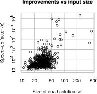
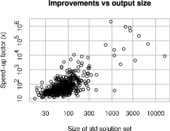
  Figure 8: Speed improvement factors for the new Algorithm 5.17

  One striking observation is how small the solution sets are, given that the triangulations range from $n=9$ to $n=25$ tetrahedra and that the sizes of the solution sets can grow exponentially in $n$. We examine this effect in greater detail in [6].

  If we focus on cases with unusually large input and output sets—those points that escape the dense clouds at the left of each plot—we find again that the improvements are particularly strong. Amongst the triangulations with input size $>100$ the improvement factors range from over $4\,000$ to over $2\,000\,000$. Likewise, with the exception of just one triangulation, those with output size $>500$ have improvements ranging from over $2\,000$ to over $2\,000\,000$. The lone exception has output size $1\,141$ and an improvement factor of $37$.

Our final tests examine the feasibility of Conjecture 5.16. Recall that this conjecture states that the running time for the quadrilateral-to-standard solution set conversion algorithm (Algorithm 5.15) is at worst polynomial in the size of the output. For this to occur we must avoid the combinatorial explosion in the sizes of the intermediate lists $L_{0},L_{1},\ldots,L_{m}$.

Figure 9 measures the extent of this combinatorial explosion. Specifically, for each triangulation we measure the size of the maximal list divided by the size of the final list—if we have a combinatorial explosion we expect this ratio to be very large, and if not then we expect it to remain close to one. We then bin these measurements into small ranges and plot the resulting frequencies in a histogram (so in each of the three plots, the sum of the heights of the bars is always 500). We take these measurements not only for Algorithm 5.15 but also for the old direct enumeration algorithm in both quadrilateral and standard coordinates.

  

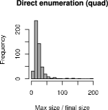
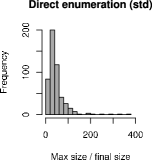
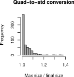
Figure 9: The combinatorial explosion for enumeration and conversion algorithms

What we see is exactly what we hope for. With the old direct enumeration algorithms, the maximal list can grow to hundreds of times the output size (and perhaps larger, recalling that for the eight worst cases the direct enumeration in standard coordinates was prematurely terminated after 30 days). For Algorithm 5.15 this ratio is never greater than $\frac{3}{2}$. That is, the behaviour we see is consistent with the intermediate lists being bounded by a linear function of the output size.

Figure 10 tests our conjecture more directly by plotting the running time of Algorithm 5.15 against the output size $k^{\prime}$ (the size of the standard solution set). Once again, both axes use a log scale so that the data points are more evenly distributed.

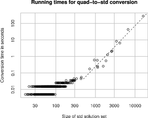
Figure 10: The running time for Algorithm 5.15 as a function of output size

It is reasonable to ignore all points where the running time is under $0.1$ seconds, since the clock resolution is only $0.01$ seconds (once again we see horizontal bands of points where the running times are the smallest that can be measured). Not only does the clock resolution introduce large relative errors for these points, but they are also highly susceptible to what would otherwise be negligible tasks, such as initialising data structures at the beginning of the algorithm, or extracting algebraic information from the triangulation.

Focusing our attention therefore on the points with time $>0.1\,\mathrm{s}$ (or equivalently, with output size $>500$), we find that the points follow what appears to be a straight line. If $t$ is the running time, this corresponds to an equation of the form $\log t=\alpha\log k^{\prime}+\beta$, or equivalently, $t\propto k^{\prime\alpha}$. That is, the time does indeed appear polynomial in the output size $k^{\prime}$.

We can measure the degree of this polynomial by performing a linear regression. This regression is indicated by the dashed line in Figure 10; its equation is approximately

$$\log t=2.4729\times\log k^{\prime}-18.5016.$$

That is, the running time appears to be a little under $t\propto k^{\prime 2.5}$. The adjusted correlation coefficient for this regression is $r\simeq 0.96$, indicating an extremely good linear fit.

Note that $t\propto k^{\prime 2.5}$ is quite reasonable, given the structure of Algorithm 5.15. If we assume that each list $L_{i}$ has size $O(k^{\prime})$, then each inductive step $L_{i}\to L_{i+1}$ involves at least $O(k^{\prime 2})$ iterations through the innermost loop (running through all $\mathbf{u}\in S_{+}$ and $\mathbf{w}\in S_{-}$). This inner loop can in turn take $O(k^{\prime})$ time as it tests for adjacency by searching for an appropriate $\mathbf{z}\in L_{r}$; however, Fukuda and Prodon [9] note that such searches often terminate early, and our additional test on the quadrilateral constraints means that many such searches can be avoided entirely. We therefore expect an average running time of between $O(k^{\prime 2})$ and $O(k^{\prime 3})$, which is precisely what we see.

One might observe that we have neglected the number of tetrahedra $n$ entirely in this empirical discussion of Conjecture 5.16. Of course $n$ features implicitly in the size of the output, since each vector in the standard solution set has dimension $7n$. We focus on $k^{\prime}$ here because it spans several orders of magnitude, ranging from 17 to 16 106; in contrast, $n$ merely ranges from 9 to 25. Since the size of the standard solution set can grow exponentially in $n$ (and this is also found to be true in the average case [6]), it is reasonable to expect $k^{\prime}$ to become the dominating factor in the running time.

Appendix: Notation

Throughout this paper we introduce a number of symbols that are used in the statements and proofs of results. For convenience, the following tables list the key symbols and where they are defined.

Sets and Vector Spaces:

Symbol Meaning Point of definition $O^{d}$ Non-negative orthant Definition 2.11 $J^{d}$ Projective hyperplane $\mathscr{S}(\mathcal{T})$ Standard projective solution space $\mathscr{Q}(\mathcal{T})$ Quadrilateral projective solution space $\mathbb{S}$ All embedded normal surfaces Notation 3.7 $\mathbb{S}_{c}$ All canonical embedded normal surfaces $\R_{a}^{7n}$, $\R_{a}^{3n}$ Admissible vectors in $\R^{7n}$ or $\R^{3n}$ $\Z_{a}^{7n}$, $\Z_{a}^{3n}$ Admissible integer vectors in $\Z^{7n}$ or $\Z^{3n}$ $\R_{a,c}^{7n}$, $\Z_{a,c}^{7n}$ Admissible canonical vectors in $\R^{7n}$ or $\Z^{7n}$ $\mathscr{A}_{r}$, $\mathscr{B}_{C}$ Used for loop invariants in Algorithm 5.15 Equations (1) and (2)

Maps:

Symbol Meaning Point of definition $\ell(\cdot)$ Vertex link (surface or vector) Definition 2.3 $\mathbf{v}(\cdot)$, $\mathbf{q}(\cdot)$ Vector representation Definition 2.4 $\overline{\,\cdot\,}$, $\overline{\mathbf{v}}(\cdot)$, $\overline{\mathbf{q}}(\cdot)$ Projective image Definition 2.12 $\sigma_{v}(\cdot)$, $\sigma_{q}(\cdot)$ Represented surface Definition 3.8 $\kappa_{s}(\cdot)$, $\kappa_{v}(\cdot)$ Canonical part (surface or vector) Definition 3.9 $\pi(\cdot)$ Quadrilateral projection Definition 3.10 $\varepsilon(\cdot)$ Canonical extension Definition 3.10 $\kappa_{v}^{(i)}(\cdot)$ Partial canonical part Definition 5.1 $\tau_{i}(\cdot)$ Truncation Definition 5.2 $\alpha(\cdot)$ Semi-admissible part Definition 5.12

References

- [1] D Avis, D Bremner, R Seidel, How good are convex hull algorithms?, Comput. Geom. 7 (1997) 265–301
- [2] A Brøndsted, An introduction to convex polytopes, Graduate Texts in Mathematics 90, Springer–Verlag, New York (1983)
- [3] B A Burton, Regina: Normal surface and –manifold topology software, http://regina.sourceforge.net/ (1999–2009)
- [4] B A Burton, Introducing Regina, the –manifold topology software, Experiment. Math. 13 (2004) 267–272
- [5] B A Burton, Optimizing the double description method for normal surface enumeration, To appear in Math. Comp., arXiv:0808.4050 (2008)
- [6] B A Burton, Extreme cases in normal surface enumeration, In preparation (2009)
- [7] M Culler, N Dunfield, FXrays: Extremal ray enumeration software, http://www.math.uic.edu/~t3m/ (2002–2003)
- [8] W Eberly, M Giesbrecht, P Giorgi, A Storjohann, G Villard, Solving sparse rational linear systems, from: “ISSAC ’06: Proceedings of the 2006 International Symposium on Symbolic and Algebraic Computation”, ACM Press (2006) 63–70
- [9] K Fukuda, A Prodon, Double description method revisited, from: “Combinatorics and Computer Science (Brest, 1995)”, Lecture Notes in Comput. Sci. 1120, Springer, Berlin (1996) 91–111
- [10] W Haken, Theorie der Normalflächen, Acta Math. 105 (1961) 245–375
- [11] W Haken, Über das Homöomorphieproblem der –Mannigfaltigkeiten. I, Math. Z. 80 (1962) 89–120
- [12] J Hass, J C Lagarias, N Pippenger, The computational complexity of knot and link problems, J. Assoc. Comput. Mach. 46 (1999) 185–211
- [13] C D Hodgson, J R Weeks, Symmetries, isometries and length spectra of closed hyperbolic three-manifolds, Experiment. Math. 3 (1994) 261–274
- [14] W Jaco, U Oertel, An algorithm to decide if a –manifold is a Haken manifold, Topology 23 (1984) 195–209
- [15] W Jaco, J H Rubinstein, –efficient triangulations of –manifolds, J. Differential Geom. 65 (2003) 61–168
- [16] W Jaco, J L Tollefson, Algorithms for the complete decomposition of a closed -manifold, Illinois J. Math. 39 (1995) 358–406
- [17] H Kneser, Geschlossene Flächen in dreidimensionalen Mannigfaltigkeiten, Jahresbericht der Deut. Math. Verein. 38 (1929) 248–260
- [18] S Matsumoto, R Rannard, The regular projective solution space of the figure-eight knot complement, Experiment. Math. 9 (2000) 221–234
- [19] T S Motzkin, H Raiffa, G L Thompson, R M Thrall, The double description method, from: “Contributions to the Theory of Games, Vol. II”, (H W Kuhn, A W Tucker, editors), Annals of Mathematics Studies 28, Princeton University Press, Princeton, NJ (1953) 51–73
- [20] J H Rubinstein, An algorithm to recognize the –sphere, from: “Proceedings of the International Congress of Mathematicians (Zürich, 1994)”, volume 1, Birkhäuser (1995) 601–611
- [21] J H Rubinstein, Polyhedral minimal surfaces, Heegaard splittings and decision problems for –dimensional manifolds, from: “Geometric Topology (Athens, GA, 1993)”, AMS/IP Stud. Adv. Math. 2, Amer. Math. Soc. (1997) 1–20
- [22] A Thompson, Thin position and the recognition problem for , Math. Res. Lett. 1 (1994) 613–630
- [23] W P Thurston, The geometry and topology of –manifolds, Lecture notes, Princeton University (1978)
- [24] S Tillmann, Normal surfaces in topologically finite –manifolds, Enseign. Math. (2) 54 (2008) 329–380
- [25] J L Tollefson, Normal surface –theory, Pacific J. Math. 183 (1998) 359–374