The WiggleZ Dark Energy Survey: small-scale clustering of Lyman Break Galaxies at $z<1$

Abstract

The WiggleZ Dark Energy Survey is a large-scale structure survey of intermediate-redshift UV-selected emission-line galaxies scheduled to cover 1000 deg², spanning a broad redshift range $0.2<z<1.0$. The main scientific goal of the survey is the measurement of baryon acoustic oscillations (BAO) in the galaxy clustering pattern at a significantly higher redshift than previous studies. The BAO may be applied as a standard cosmological ruler to constrain dark energy models. Based on the first $20\%$ of the dataset, we present initial results concerning the small-scale clustering of the WiggleZ targets, together with survey forecasts. The WiggleZ galaxy population possesses a clustering length $r_{0}=4.40\pm 0.12\,h^{-1}$ Mpc, which is significantly larger than $z=0$ UV-selected samples, with a slope $\gamma=1.92\pm 0.08$. This clustering length is comparable to $z=3$ Lyman Break Galaxies with similar UV luminosities. The clustering strength of the sample increases with optical luminosity, UV luminosity and reddening rest-frame colour. The full survey, scheduled for completion in 2010, will map an effective volume $V_{\rm eff}\approx 1$ Gpc³ (evaluated at a scale $k=0.15\,h$ Mpc^-1) and will measure the angular-diameter distance and Hubble expansion rates in three redshift bins with accuracies $\approx 5\%$. We will determine the value of a constant dark energy equation-of-state parameter, $w_{\rm cons}$, with a higher precision than existing supernovae observations using an entirely independent technique. The WiggleZ and supernovae measurements lie in highly complementary directions in the plane of $w_{\rm cons}$ and the matter density $\Omega_{\rm m}$. The forecast using the full combination of WiggleZ, supernovae and CMB datasets is a marginalized error $\Delta w_{\rm cons}=0.07$, providing a robust and precise measurement of the properties of dark energy including cross-checking of systematic errors.

1 Introduction

The large-scale structure of the Universe is one of the pillars of our modern understanding of cosmology, encoding information about the contents and evolution of the Universe, the physics of the growth of density fluctuations with time, and the formation and evolution of galaxies within the underlying network of dark matter haloes. In particular, the large-scale clustering pattern of galaxies is sensitive to the properties of the cosmic dark energy component which is currently poorly understood. Dark energy influences both the rate of growth of structure and the geometrical distance-redshift relations. One of the cleanest probes of dark energy is to delineate as a function of redshift the apparent tangential and radial size of the baryon acoustic oscillation scale, a known “standard ruler” preferred separation imprinted into the galaxy distribution (Cooray et al. 2001; Eisenstein 2002; Blake & Glazebrook 2003; Seo & Eisenstein 2003; Hu & Haiman 2003; Linder 2003; Glazebrook & Blake 2005). This cosmological probe is helping to motivate a new generation of massive spectroscopic galaxy surveys.

Cosmic structure has been mapped out by a succession of galaxy redshift surveys of increasing size and depth. The local Universe (redshifts $z<0.2$) has been studied in exquisite detail by the 2-degree Galaxy Redshift Survey (2dFGRS; Colless et al. 2001) and the Sloan Digital Sky Survey (SDSS; York et al. 2000). The SDSS Luminous Red Galaxy component extended this programme to a mean redshift $z\approx 0.35$ using a specific type of tracer galaxy (Eisenstein et al. 2001). Indeed, the cosmological conclusions reached should be independent of the galaxy type used, given that the “bias” with which galaxies trace the underlying dark matter fluctuations is expected to be a simple linear function on large scales (Coles 1993; Scherrer & Weinberg 1998). In this sense, the choice of the “tracer population” of galaxies can be determined by observational considerations such as telescope exposure times, the availability of input imaging data for target selection, and secondary science goals.

The WiggleZ Dark Energy Survey, using the AAOmega multi-object spectrograph at the 3.9m Anglo-Australian Telescope (AAT), is designed as the next leap forwards in redshift coverage, targetting the range $0.2<z<1.0$. The survey is scheduled to cover a sky area of 1000 deg², mapping a cosmic volume $V\sim 1$ Gpc³ sufficient to measure the imprint of baryon oscillations in the clustering pattern at a significantly higher redshift than has been previously achieved by 2dFGRS (Cole et al. 2005; Percival et al. 2007) and SDSS (Eisenstein et al, 2005; Huetsi 2006; Percival et al. 2007; Gaztanaga et al. 2008). The survey redshift range is motivated by the optimal redshift location for testing a cosmological constant model in a spatially-flat Universe (Parkinson et al. 2007), which is the sensible initial hypothesis to reject in the dark energy parameter space. The target galaxy population is bright emission-line galaxies selected from UV imaging by the Galaxy Evolution Explorer (GALEX) satellite (Martin et al. 2005). This choice is motivated by the short (1-hr) exposure times required to obtain redshifts at the AAT. The survey commenced in August 2006 and is scheduled to finish in July 2010, using the equivalent of 165 clear nights of telescope time (220 awarded nights). Secondary science goals involve the study of star formation and galaxy evolution as a function of redshift and environment.

In this initial study we focus on the small-scale clustering properties of the first $20\%$ of the WiggleZ sample. The clustering strength is an important parameter in the survey design and cosmological parameter forecasts: the signal-to-noise with which we can recover the galaxy power spectrum depends on the bias of the galaxies with respect to the dark matter fluctuations, which affects the balance between sample variance and shot noise in the power spectrum error budget. These initial clustering measurements allow us to determine the bias parameter and complete the survey forecast.

Furthermore, the joint UV-optical selection in the redshift interval $0.2<z<1$ places the WiggleZ survey in an interesting location in the parameter space of galaxy evolution. In this context, the clustering strength of a set of galaxies provides a direct indication of the density of the environment or (equivalently) the typical mass of the dark matter haloes hosting the galaxies. The clustering strength of UV-selected samples has been studied at low redshift $z\approx 0$ (Milliard et al. 2007; Heinis et al. 2007) and the corresponding rest-frame samples have been selected at much higher redshift $z\approx 3$ through studies of the clustering of Lyman Break Galaxies (LBGs; e.g. Giavalisco & Dickinson 2001; Ouchi et al. 2001; Arnouts et al. 2002; Foucaud et al. 2003; Adelberger et al. 2005; Allen et al. 2005; Ouchi et al. 2005; Lee et al. 2006; Yoshida et al. 2008). The WiggleZ survey samples a redshift range which is intermediate to these previous studies. Moreover, the clustering strength of optically-selected star-forming galaxies at high redshift has been studied over small areas by the Deep Extragalactic Evolutionary Probe (DEEP2) project (Coil et al. 2008) and the VIMOS VLT Deep Survey (VVDS; Meneux et al. 2006). WiggleZ is mapping an area $\sim 100$ times larger, and is therefore able to measure accurately the clustering strength of the most luminous star-forming galaxies, for which these smaller surveys are limited by small-number statistics and sample variance.

The backdrop to these studies is the recent concept of “down-sizing” (Cowie et al. 1996; Glazebrook et al. 2004; van Dokkum et al. 2004) whereby the stars in more massive galaxies appear to have formed earlier, and the typical mass of the most actively star-forming galaxies is expected to decrease with time. A recent study of LBGs (Yoshida et al. 2008) has emphasized the importance of studying the clustering segregration with both UV and optical luminosities, which crudely trace ongoing star formation rate and stellar mass, respectively. WiggleZ is well-suited for undertaking such studies over the redshift range $0.2<z<1.0$.

Figure 1: The sky distribution of the seven WiggleZ survey regions compared to the coverage of the SDSS, RCS2 and GALEX Medium Imaging Survey at the end of 2008.

The plan of this paper is as follows: in Section 2 we introduce the WiggleZ survey strategy and target selection and describe the data sample used in this study. In Section 3 we describe the methodology used to produce the small-scale clustering measurement including the generation of random (unclustered) realizations of the dataset with the correct selection functions and redshift completeness map. We also explain how we derive the statistical error in the clustering measurement. We present the clustering results in Section 4 (split by redshift, absolute magnitude and rest-frame colour) together with initial comparisons to other studies. Section 5 contains the cosmological parameter forecasts for the full WiggleZ survey, and Section 6 summarizes our conclusions. When converting redshifts to co-moving co-ordinates we assume a spatially-flat Universe with cosmological parameters $\Omega_{\rm m}=0.3$ and $\Omega_{\Lambda}=0.7$.

2 Data

The design and implementation of the WiggleZ Dark Energy Survey will be fully described in a forthcoming “survey paper” (Drinkwater et al. 2009, in preparation) which will accompany our mid-term Data Release. We include a brief outline here both for ease of reference and to emphasize the key points relevant to the small-scale clustering analysis.

2.1 WiggleZ survey strategy

The WiggleZ survey strategy is to harvest low signal-to-noise spectra of a large number of UV-selected emission-line galaxies in relatively short exposure times (1-hr integrations at the AAT). The survey tolerates a relatively low redshift completeness of $70\%$ but generates a large statistical sample of galaxy redshifts. The survey goal is to cover $1{,}000$ deg² of the equatorial sky, gathering $\sim 350{,}000$ spectra of which $\sim 245{,}000$ are expected to yield successful redshifts. The survey was designed such that the average galaxy number density $n$ is related to the amplitude of the galaxy clustering power spectrum $P_{\rm gal}$ on the relevant baryon oscillation scales by $n\sim 1/P_{\rm gal}$, implying that the contributions of sample variance and shot noise to the clustering error are equal. This is the optimal survey strategy for fixed number of galaxies.

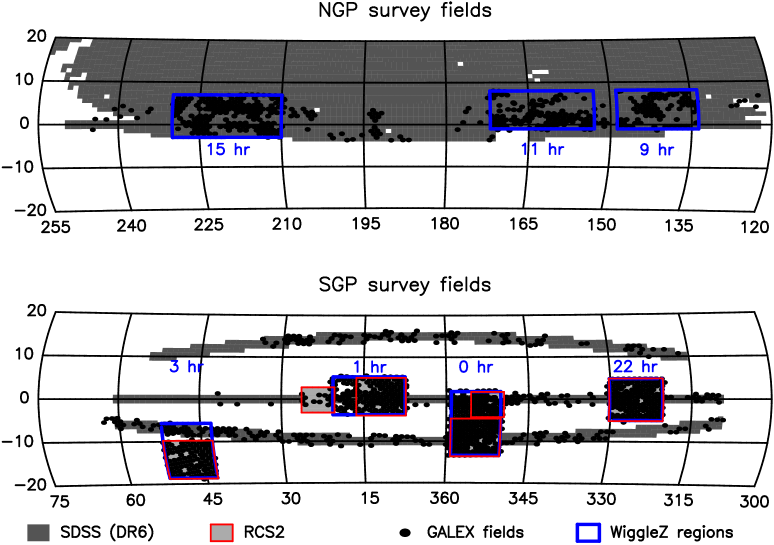
The WiggleZ survey area, illustrated in Figure 1, is split into seven equatorial regions to facilitate year-round observing. We require that each region should possess a minimum angular dimension of $\sim 10$ deg, corresponding to a spatial co-moving scale that exceeds by at least a factor of two the standard ruler preferred scale [which projects to (8.5, 4.6, 3.2, 2.6) deg at $z=(0.25,0.5,0.75,1.0)$]. The survey coverage within individual regions should also be highly ($>70\%$) contiguous, otherwise the significance of the detection of the acoustic features is degraded by convolution with the survey window function. The survey duration is forecast to be $\sim 165$ clear nights between August 2006 and July 2010, using the multi-object capability of the 2dF positioner system coupled to the AAOmega spectrographs (Saunders et al. 2004; Sharp et al. 2006).

Galaxy redshifts are obtained from the bright emission lines associated with star-forming galaxies, in particular redshifted [OII] 3727Å, H$\beta$ 4861Å  and [OIII] 4959Å, 5007Å. Low-resolution (5Å FWHM) spectra are obtained spanning the (observed-frame) wavelength range $5500-9500$Å, hence the majority of successful redshifts in the range $z<0.95$ are confirmed by multiple emission lines. Single-line redshifts are almost invariably [OII], for which we usually resolve the doublet in the range $z>0.8$, increasing our confidence in the line identification. Redshifts are obtained by visual inspection of each spectrum using the interactive software tool “runz”, and are classified by a quality flag $1\leq Q\leq 5$, where the range $Q\geq 3$ denotes a “reliable” redshift (see Colless et al. 2001). The fraction of stellar contamination is very small ($<1\%$) and we find a similarly low fraction of high-redshift quasar interlopers. The galaxy continuum is typically detected with low signal-to-noise (an average of $S/N\sim 1$ per resolution element).

2.2 WiggleZ survey target selection

WiggleZ targets are chosen by a joint UV-optical selection. The primary selection dataset is the Medium Imaging Survey undertaken by the Galaxy Evolution Explorer (GALEX) UV satellite, which provides typical exposure times of 1500 seconds in two filter bands, $FUV$ ($1350-1750$Å) and $NUV$ ($1750-2750$Å). The GALEX point-spread function is too broad to allow for accurate placement of the spectrograph optical fibres, therefore the UV imaging is cross-matched with optical data. For our NGP regions, the SDSS imaging data are used. For our SGP regions, the SDSS $2.5^{\circ}$ stripes are too narrow compared to the preferred baryon oscillation scale hence we use imaging data from the second Red Cluster Sequence (RCS2) project instead (Yee et al. 2007). Sources are cross-matched between the GALEX and optical catalogues with a matching tolerance of 2.5 arcsec (which produces a negligible fraction of incorrect matches). In each imaging dataset, the majority of galaxies possess relatively low signal-to-noise ($S/N=3-5$) but their detection in both datasets ensures a robust sample. We note that acquisition of our eventual requirement of $\sim 1250$ GALEX orbits of data is still ongoing. About $70\%$ of this total had been obtained at the end of 2008.

Targets are chosen from the UV-optical matched sample using a series of magnitude and colour cuts. These cuts are tuned to optimize the fraction of targets lying at high redshift $z>0.5$. Firstly the galaxy magnitudes are de-reddened using standard dust corrections based on the local value of $E(B-V)$ measured from the Schlegel, Finkbeiner & Davis (1998) dust maps. The primary GALEX selection criterion is a red $FUV-NUV$ colour ($FUV-NUV>1$ or $FUV$ drop-out), motivated by the Lyman Break passing through the $FUV$ filter for $z>0.5$, and tuned by looking at galaxy templates. At the depth of the Medium Imaging Survey this colour is noisy, resulting in a significant amount of contamination by low-redshift ($z<0.5$) galaxies which are partially removed by the additional cuts described below. We also impose a faint UV magnitude limit $NUV<22.8$ and an additional signal-to-noise requirement $S/N>3$ for the detected NUV flux (which becomes relevant for fields with unusually high dust content or low exposure time). The GALEX field-of-view is circular with radius $\sim 0.6$ deg; we only select sources within the central $0.55$ deg because of concerns over the photometry at the edge of the field.

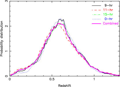
Our primary optical selection cuts are derived from SDSS $r$-band imaging. We require a UV-optical colour in the range $-0.5<NUV-r<2$ based on the expected model tracks of star-forming galaxies. We impose a bright $r$-band limit $20<r<22.5$; the UV-optical colour cut implies that the median optical magnitude of our targets is $r\sim 21.5$. Finally we increase the high-redshift efficiency by introducing optical colour cuts. Different cuts are used for the SDSS and RCS2 regions, governed by the available imaging bands and depths. For the SDSS regions analyzed in this paper, we apply cuts for those (brighter) galaxies with good detections in the SDSS $g$- and $i$-bands. Specifically, for targets with $g<22.5$ and $i<21.5$ we reject galaxies in the colour space defined by $r-i<g-r-0.1$ and $r-i<0.4$ which is occupied by low-redshift galaxies both theoretically and empirically (more details will be given in Drinkwater et al. 2009, in preparation). The final fraction of $z>0.5$ galaxies obtained is $\approx 70\%$. The redshift distribution is displayed in Figure 2.

An average of 3-4 pointings of the 2dF spectrograph per patch of sky is required in order to achieve the required target density of 350 deg^-2. For any observing run the optimal placement of field centres (based on the current availability of targets) is achieved using the “Metropolis” (simulated annealing) algorithm (Campbell, Saunders & Colless 2004). Galaxies are prioritized for spectroscopic follow-up on the basis of optical $r$-band magnitude, in the sense that fainter targets are observed first. The motivation for this strategy is to combat the potential inefficiency of “mopping up” residual galaxies in the final pointing for any patch of sky: the brighter remaining galaxies can be observed in a shorter exposure time by configuring fewer fibres.

2.3 WiggleZ July 2008 data sample

In this paper we analyze the subset of the WiggleZ sample assembled from our first observations in August 2006 up until the end of the 08A semester (July 2008). At this point we had utilized 108 of our allocated nights, of which the equivalent of 70 nights were clear. The available galaxy database included $\approx 97{,}000$ reliable ($Q\geq 3$) WiggleZ unique galaxy redshifts.

In this analysis we only use those galaxies lying in the SDSS regions of our optical imaging because work is still on-going on the RCS2 portion of the angular selection function. Specifically, we include the WiggleZ 9-hr, 11-hr, 15-hr and 0-hr (SDSS) regions illustrated in Figure 1. The number of existing AAOmega pointings in these regions is (42, 98, 140, 48). The numbers of galaxies in each region with reliable redshifts satisfying the final survey selection criteria are (5782, 14873, 21629, 4383), constituting a total sample of $N=46{,}667$ for this initial analysis (about $20\%$ of the final sample).

3 Analysis

3.1 Correlation function estimator

We quantify the small-scale clustering of the galaxy distribution using a standard set of techniques based on the 2-point correlation function. This statistic compares the number of observed close galaxy pairs to that expected by random chance, as a function of spatial separation. The key requirement is an ensemble of random (unclustered) realizations of the survey possessing the same selection function as the observed galaxy distribution. With this in place we convert the data (D) and random (R) galaxy angle-redshift distributions into a grid of co-moving co-ordinates $(x,y,z)$ using an assumed cosmological model (we use a flat model with $\Omega_{\rm m}=0.3$). We then bin the number of data-data (DD), data-random (DR) and random-random (RR) pairs in the two-dimensional space of separation perpendicular to the line-of-sight (denoted by $\sigma$) and parallel to the line-of-sight (denoted by $\pi$). This decomposition is motivated by the influence of galaxy peculiar velocities (redshift-space distortions) which shift galaxies in $\pi$, but not in $\sigma$. Each of our random realizations contains the same number of targets as the data sample, and is generated by a method described below. The pair counts $DR$ and $RR$ are determined by averaging over 10 random realizations.

The 2D redshift-space correlation function $\xi_{z}(\sigma,\pi)$ is derived using the estimator proposed by Landy & Szalay (1993):

$$\xi_{z}(\sigma,\pi)=\frac{DD(\sigma,\pi)-2\,DR(\sigma,\pi)+RR(\sigma,\pi)}{RR(\sigma,\pi)}$$ (1)

(where this last equation assumes an equal number of data and random galaxies). We bin galaxy pairs by the absolute value of the line-of-sight separation, i.e. $\pi\equiv|\pi|$. The “real-space” correlation function (independent of the redshift-space distortion) can be obtained by summing equation 1 over $\pi$. We first define the projected correlation function $\Xi(\sigma)$ (Davis & Peebles 1983):

$$\Xi(\sigma)=2\sum_{\pi=0}^{\infty}\xi_{z}(\sigma,\pi)\,\Delta\pi$$ (2)

where the factor of 2 extrapolates the result to the full range $-\infty<\pi<\infty$. If we assume that the real-space correlation function $\xi_{r}$ is well-described by a power-law $\xi_{r}(r)=(r_{0}/r)^{\gamma}$, where $r_{0}$ is the clustering length, $\gamma$ is the slope and $r=\sqrt{\sigma^{2}+\pi^{2}}$, and if we neglect the coherent infall velocities described below, we can then derive

$$\xi_{r}(r)=\frac{\Xi(r)}{r\,C_{\gamma}}$$ (3)

where

$$C_{\gamma}=\int_{-\infty}^{\infty}(1+u^{2})^{-\gamma/2}du=\frac{\Gamma(\frac{1}{2})\Gamma(\frac{\gamma-1}{2})}{\Gamma(\frac{\gamma}{2})}$$ (4)

The difficulty with this method is that the measurement of $\xi_{z}(\sigma,\pi)$ becomes noisy for large $\pi$ and therefore the summation in equation 2 must be truncated at some $\pi=\pi_{\rm max}$, invalidating equation 3. We therefore adopted the following approach (similar to the methodology of Coil et al. 2008) to convert a model real-space correlation function $\xi_{r}(r)=(r_{0}/r)^{\gamma}$ into a projected correlation function which may be compared with the data. In the linear regime, the effect of coherent infall velocities on the correlation function can be modelled by

$$\xi_{z}(\sigma,\pi)=\xi_{0}(r)P_{0}(\mu)+\xi_{2}(r)P_{2}(\mu)+\xi_{4}(r)P_{4}(\mu)$$ (5)

where $P_{\ell}(\mu)$ are the Legendre polynomials, $\mu=\cos{\theta}$ and $\theta$ is the angle between $r$ and $\pi$. For a power-law real-space correlation function,

$$\xi_{0}(r) = \left(1+\frac{2\beta}{3}+\frac{\beta^{2}}{5}\right)\xi_{r}(r)$$ (6)

$$\xi_{2}(r) = \left(\frac{4\beta}{3}+\frac{4\beta^{2}}{7}\right)\left(\frac{\gamma}{\gamma-3}\right)\xi_{r}(r)$$ (7)

$$\xi_{4}(r) = \frac{8\beta^{2}}{35}\left[\frac{\gamma(2+\gamma)}{(3-\gamma)(5-\gamma)}\right]\xi_{r}(r)$$ (8)

where $\beta\approx\Omega_{\rm m}(z)^{0.55}/b$ is the redshift-space distortion parameter (Hamilton 1992; Hawkins et al. 2003) and $b$ is the linear galaxy bias parameter. We assumed $\beta=0.6$ for this model, consistent with our measurements (see Section 4.3), and for each set of trial values $(r_{0},\gamma)$ we employed the above set of equations to calculate $\xi_{z}(\sigma,\pi)$. For each value of $\sigma$ we then integrated this function in the $\pi$ direction up to $\pi=\pi_{\rm max}$ in order to compare with the correlation function measurements. We assumed $\pi_{\rm max}=20\,h^{-1}$ Mpc, and we checked that our results did not depend sensitively on the value of $\pi_{\rm max}$.

Figure 2: The redshift probability distribution of WiggleZ targets with reliable redshifts in the four survey regions analyzed in this study (normalized such that $\int P(z)\,dz=1$). We plot cubic spline fits to the redshift distribution. We also show the result for the combined regions as the thicker line.

We treated each of the four survey regions independently, measuring the correlation function and corresponding error. We then constructed the “combined” correlation function by averaging the measurements in the four regions with inverse-variance weighting. For convenience, we plot projected correlation functions in this paper as $\Xi(\sigma)/(\sigma\,C_{\gamma,{\rm reduced}})\propto(r_{0}/\sigma)^{\gamma}$, where

$$C_{\gamma,{\rm reduced}}=\int_{-\sigma/\pi_{\rm max}}^{\sigma/\pi_{\rm max}}(1+u^{2})^{-1/2}du$$ (9)

3.2 Selection function

We now discuss the generation of the random survey realizations that are required for calculation of the correlation function. This determination of the survey “selection function” will be described fully in a forthcoming paper (Blake et al. 2009, in preparation) and we give a brief summary here.

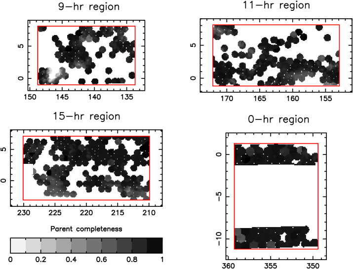
The calculation begins with the angular selection function of the “parent” sample of UV-optical matches. This function is defined firstly by the boundaries of the GALEX fields and SDSS coverage map. Secondly, because the UV magnitudes of our sample lie close to the threshold of the GALEX MIS observations, there is a significant incompleteness in the GALEX imaging that depends on the local dust extinction and GALEX exposure time. We used the GALEX number counts as a function of dust and exposure time to calibrate the relation between these quantities and the parent WiggleZ target density. This angular completeness function is displayed in Figure 3 for the four survey regions analyzed in this paper. We used this map to produce a series of random realizations of the parent catalogue for each region.

Figure 3: Greyscale map illustrating the angular completeness of the parent catalogue of SDSS-GALEX matches for the four survey regions analyzed in this paper. This parent target density varies with dust extinction and GALEX exposure time because the UV magnitudes of WiggleZ galaxies lie close to the threshold of the Medium Imaging Survey data. The $x$-axis and $y$-axis of each panel are right ascension and declination, respectively.

The next step is to process these random parent catalogues into random realizations of the redshift catalogue. The spectroscopic follow-up of the parent catalogue comprises a network of overlapping AAOmega pointings, with field centres optimized by the simulated annealing algorithm and not lying on a regular grid. The fraction of successful redshifts in each pointing varies considerably depending on weather conditions. Furthermore, the redshift completeness within each AAOmega field exhibits a significant radial variation due to acquisition errors at the plate edges.

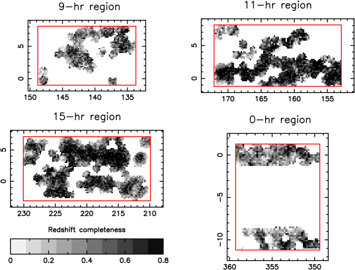
In Figure 4 we illustrate how the redshift completeness varies across these survey regions by simply taking the ratio of successful redshifts to parent galaxies in each pixel. This is a useful visualization, but in fact the number of unique sectors defined by the overlapping AAOmega fields is so large that this determination of the redshift completeness map is very noisy. Indeed, some unique sectors contain zero parent galaxies.

Figure 4: Greyscale map illustrating the completeness of the spectroscopic follow-up of the WiggleZ targets shown in Figure 3 for the four survey regions analyzed in this paper. This Figure is generated by taking the ratio of the galaxy densities in the redshift and parent catalogues in small cells. In our clustering analysis a more accurate approach is adopted in which the full AAOmega pointing sequence is applied to random realizations of the parent catalogue. The $x$-axis and $y$-axis of each panel are right ascension and declination, respectively.

One possible approach is to smooth this completeness map over larger areas to reduce the Poisson noise at the expense of a diminished sensitivity to small-scale completeness variations between AAOmega pointings. In this analysis we use an alternative approach, which is to apply the AAOmega pointing sequence to each of the random realizations of the parent catalogue, and thereby create an ensemble of random realizations of the redshift catalogue. The AAOmega pointing sequence is defined by the right ascension and declination of the field centre together with the number of successful and unsuccessful redshifts obtained for that pointing. Within each field centre parent galaxies are chosen randomly to create the synthetic redshift catalogue. It is also necessary to track the sky coverage of the GALEX data which was contemporaneous with each AAOmega pointing. Because the acquisition of the GALEX imaging data is ongoing with the spectroscopic follow-up, the boundaries of the angular mask must be modulated in step with the redshift follow-up. In addition we impose the radial redshift completeness variation across each AAOmega field, measured independently for each observing run.

The redshift distribution $N(z)$ of observed galaxies varies with position in the sky. This is due to the magnitude prioritization described in Section 2.2. Because galaxies with fainter $r$-band magnitudes are targeted first, the $N(z)$ will be skewed toward higher redshifts for areas of the survey which have been targeted by fewer AAOmega observations. This dependence is accounted for in our random catalogues by measuring the magnitude distribution of targeted galaxies as a function of sky position and drawing a random redshift from the correctly weighted $N(z)$.

3.3 Fibre collision correction

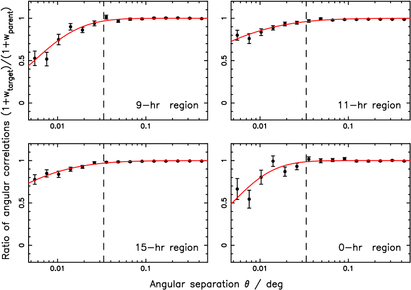
The optical fibres of the 2dF spectrograph cannot be placed closer together than $0.5$ arcmin, and there is a diminishing probability of observing in a single pointing both members of a close pair of parent galaxies separated by an angular distance of less than 2 arcmin [a projected spatial distance of $(0.4,0.8,1.1,1.4)\,h^{-1}$ Mpc at $z=(0.25,0.5,0.75,1.0)$]. This restriction will eventually be ameliorated by the requirement of observing each patch of sky with 3-4 AAOmega pointings to build up the number density of the redshift catalogue. At present, however, there is a deficit of close angular pairs in the redshift catalogue, which artificially suppresses the measured value of the galaxy correlation function on small scales. The close angular pair deficit is illustrated in Figure 5 by plotting the ratio $(1+w_{t})/(1+w_{p})$ as a function of angular separation $\theta$, where $w_{t}$ and $w_{p}$ are the angular correlation functions of the targeted catalogue and the parent catalogue, respectively. This ratio provides the fraction of surviving close pairs. In order to correct the galaxy correlation function for the missing close pairs we increased the contribution of each galaxy pair to the data-data pair count as a function of angular separation by a factor $(1+w_{p})/(1+w_{t})$ (the inverse of the quantity plotted in Figure 5) using a 2-parameter model $\{1+{\rm erf}[({\rm log_{10}}\theta-\mu)/\sigma]\}/2$ fitted to the data in Figure 5.

We note that for a survey with a redshift-dependent galaxy number density $n(z)$, the minimum-variance correlation function measurement for separation $s$ is achieved if galaxies are assigned a redshift-dependent weight $w(z)=[1+4\pi n(z)J_{3}(s)]^{-1}$ where $J_{3}(s)=\int_{0}^{s}\xi(x)\,x^{2}\,dx$ (Efstathiou 1988; Loveday et al. 1995). In our case the galaxy number density is sufficiently low that $w(z)\approx 1$ and this weighting makes a negligible difference to the results and we do not use it.

Figure 5: The ratio of the angular correlation functions of the WiggleZ parent catalogue and targeted catalogue for the four survey regions analyzed in this paper. This ratio indicates the fraction of close pairs surviving the restrictions of fibre collisions as a function of angular scale; pairs are lost for angular separations less than $\theta=2$ arcmin which is indicated by the vertical dashed line. The solid curve indicates the best fit of the 2-parameter model $\{1+{\rm erf}[({\rm log_{10}}\theta-\mu)/\sigma]\}/2$.

3.4 Redshift blunder correction

The low signal-to-noise spectra obtained by the WiggleZ survey imply that a small but significant fraction of galaxies are assigned a “reliable” ($Q\geq 3$) redshift which proves to be incorrect owing to emission-line mis-identification. This is monitored in the survey by allocating a small number of fibres (typically 3 to 5 out of 400 per pointing) to re-observe galaxies with existing $Q\geq 3$ redshifts. The fraction of repeat observations producing a discrepant redshift may be used to estimate the redshift “blunder” rate.

There is a significant difference in the reliability of $Q=3$ redshifts and $Q\geq 4$ redshifts. $Q=3$ redshifts (which represent a fraction $32\%$ of reliable redshifts) are typically based either on noisy spectra or on a single emission line with no confirming spectral features, whereas $Q\geq 4$ redshifts are based on multiple detected emission lines. Comparing repeat observations consisting of a $Q=3$ redshift and a $Q\geq 4$ redshift, assuming that the latter provides the correct redshift identification, we conclude that $\approx 17\%$ of $Q=3$ redshifts are blunders. This agrees with the internal discrepancy rate amongst repeated pairs of $Q=3$ redshifts (which is $31\%$, which must be divided by two to obtain the blunder rate per object). Comparing repeat observations consisting of $Q\geq 4$ redshifts we find that only $\approx 1\%$ of these redshifts are blunders.

The blunder rate for $Q=3$ spectra varies significantly with the true galaxy redshift, which determines how many emission lines appear in the observed wavelength range. The dependence is displayed in Figure 6 based on the comparison of $Q=3$ and $Q\geq 4$ pairs of repeat observations. The total blunder rate for all reliable ($Q\geq 3$) redshifts is below $5\%$ for the range $z<0.7$, increasing to $20\%$ by $z=1$. The redshift blunder rate does not depend on galaxy continuum magnitude.

Figure 6: The dependence of the redshift blunder rate of galaxies with $Q=3$ spectra on the (true) galaxy redshift, determined by comparing repeat observations consisting of pairs of spectra with $Q=3$ and $Q\geq 4$. Poissonian error bars are shown.

Redshift mis-identification reduces the measured value of the galaxy correlation function because a fraction of true close data-data pairs are lost as one or both of the redshifts is randomized. If $f_{\rm bad}$ is the redshift blunder rate, the correction to the correlation function is a constant factor $(1-f_{\rm bad})^{-2}$ assuming the blunder redshift is randomly distributed. We applied this correction to the measured correlation function to deduce the final value:

$$\xi_{z}(\sigma,\pi)_{\rm corrected}=\xi_{z}(\sigma,\pi)_{\rm measured}\times(1-f_{\rm bad})^{-2}$$ (10)

When measuring the galaxy correlation function for a particular redshift or luminosity range, we re-calculated the redshift blunder rate for the corresponding sample in each region as explained below. We corrected the correlation function for that region using Equation 10, before combining together the correlation functions for the different regions. We determined the redshift blunder rate for each region by weighting the blunder probabilities of the $N$ individual objects in that region:

$$f_{\rm bad}=\frac{1}{N}\left(\sum_{i=1}^{N}f_{{\rm bad},i}\right)$$ (11)

For objects with $Q=3$ we assigned the probability for each object based on its redshift using Figure 6. For objects with $Q\geq 4$ we assumed a blunder rate of $1\%$.

3.5 Jack-knife re-samples

In order to determine the error in the measured correlation function we must characterize the statistical fluctuations in the data sample. It is well-known that these fluctuations are not well-described by Poisson statistics, for which the error in the pair count $DD$ in a separation bin would be equal to $\sqrt{DD}$. Sample variance, geometrical edge effects and the same galaxy participating in pairs in different separation bins cause the statistical variance of the galaxy pair count to exceed the Poisson prediction and induce covariances between the bins.

In this analysis we use jack-knife re-sampling to determine the correlation function error. In this technique the dataset is divided into $N$ equal-area sub-regions on the sky. The correlation function analysis is repeated $N$ times, in each case omitting one of the sub-regions in turn. Labelling the different correlation function measurements at separation $s$ as $\xi_{i}(s)$ from $i=1$ to $i=N$, the covariance between separation bins $j$ and $k$ was deduced as:

$$C_{jk} \equiv \left<\xi(s_{j})\,\xi(s_{k})\right>-\left<\xi(s_{j})\right>\left<\xi(s_{k})\right>$$ (12)

$$\approx (N-1)\left(\frac{\sum_{i=1}^{N}\xi_{i}(s_{j})\xi_{i}(s_{k})}{N}-\overline{\xi(s_{j})}\overline{\xi(s_{k})}\right)$$ (13)

where $\overline{\xi(s_{j})}=\sum_{i=1}^{N}\xi_{i}(s_{j})/N$. The factor $(N-1)$ in equation 13 is required because the jack-knife re-samples are not independent, sharing a high fraction of common sources.

We defined the jack-knife samples by splitting each survey region into $N=49$ sub-regions using constant boundaries of right ascension and declination. We tried the alternative technique of using the GALEX tiles to define the jack-knife regions; this produced a result that did not differ significantly. Future analyses of the WiggleZ survey clustering will quantify the statistical fluctuations using mock galaxy catalogues constructed from N-body simulations.

4 Results

4.1 2D correlation function

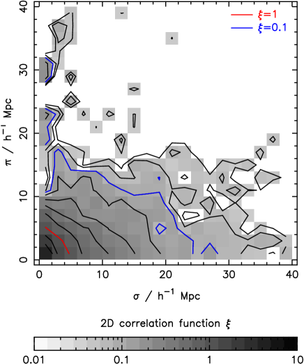
Figure 7 illustrates the dependence of the 2D redshift-space correlation function $\xi_{z}(\sigma,\pi)$ of equation 1 on the separations $\pi$ and $\sigma$ perpendicular and parallel to the line-of-sight for the sample of WiggleZ galaxies spanning the full redshift range $0.1<z<1.3$. We measured the correlation function separately for the four independent survey regions and combined the results using inverse-variance weighting. The non-circularity of the contours of constant $\xi_{z}$ trace the imprint of galaxy peculiar velocities; we use linear scales of $\sigma$ and $\pi$ in this plot to focus on the large-scale distortions. In particular, for scales $>10\,h^{-1}$ Mpc the increase in the value of $\xi_{z}$ with increasing angle to the line-of-sight $\theta={\rm arctan}(\sigma/\pi)$ for fixed total separation $\sqrt{\sigma^{2}+\pi^{2}}$ is a signature of coherent galaxy infall and can be quantified to measure the redshift-space distortion parameter $\beta$ (see Section 4.3). We also detect some evidence for “fingers of god”, in the form of elongation of the contours of $\xi_{z}$ along the $\pi$-axis, due to the virialized motions of galaxies in clusters. There is some similarity here with the results of Coil et al. (2008) Figure 7 for luminous blue galaxies, except that our sample size is significantly larger.

Figure 7: The 2D redshift-space correlation function $\xi_{z}(\sigma,\pi)$ as a function of separation $\sigma$ perpendicular to the line-of-sight and $\pi$ parallel to the line-of-sight. The function is represented using both greyscale and contours. Results for the four survey regions analyzed in this paper have been combined for the galaxy redshift range $0.1<z<1.3$. The non-circularity of the contours encodes the imprint of galaxy peculiar velocities, as discussed in the text. The red line (3rd contour from the bottom left) is the $\xi_{z}=1$ contour which lies at approximately $\sqrt{\sigma^{2}+\pi^{2}}\approx 5\,h^{-1}$ Mpc; the blue line (8th contour from the bottom left) is the $\xi_{z}=0.1$ contour.

4.2 Clustering length of the sample

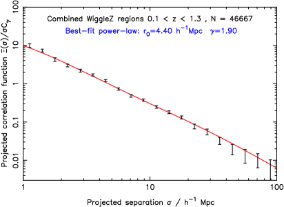
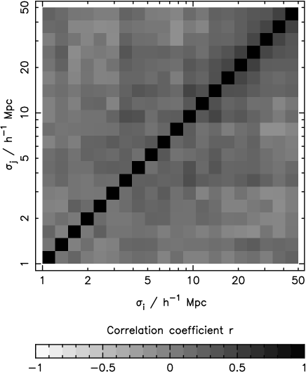
Galaxy peculiar velocities change values of $\pi$ but not $\sigma$. The real-space clustering properties of the galaxies may therefore be deduced by integrating $\xi_{z}(\sigma,\pi)$ along the $\pi$-axis, as discussed in Section 3.1. We summed the 2D correlation function for the $0.1<z<1.3$ sample in 5 logarithmic bins of $\pi$ between $\pi_{\rm min}=0.5\,h^{-1}$ Mpc and $\pi_{\rm max}=20\,h^{-1}$ Mpc. The result is plotted in Figure 8 for the projected separation range $1<\sigma<100\,h^{-1}$ Mpc, with errors obtained from the jack-knife re-sampling. The full covariance matrix $C$ deduced from the jack-knife re-samples is displayed in Figure 9 by plotting in greyscale the correlation coefficient between two separation bins $i$ and $j$:

$$r(i,j)=\frac{C_{ij}}{\sqrt{C_{ii}\,C_{jj}}}$$ (14)

Figure 8: The projected correlation function $\Xi(\sigma)/\sigma C_{\gamma}$ as a function of projected separation $\sigma$ for galaxies in the redshift range $0.1<z<1.3$, combining the results for the four survey regions analyzed in this paper. The solid line is the best-fitting power-law for the separation range $1.5<\sigma<15\,h^{-1}$ Mpc. The $y$-axis is normalized by a factor which produces numerical results approximating $(r_{0}/\sigma)^{\gamma}$.

Figure 9: Greyscale plot of the correlation coefficient $r$ of equation 14, indicating the degree of covariance between different separation bins for each redshift slice.

We employed the methodology of Section 3.1 to fit a power-law real-space correlation function $\xi_{r}=(r_{0}/r)^{\gamma}$ to the redshift-space data over the range $1.5<\sigma<15\,h^{-1}$ Mpc, by minimizing the $\chi^{2}$ statistic using the covariance matrix:

$$\chi^{2}=\sum_{i,j}\delta y_{i}\,(C^{-1})_{ij}\,\delta y_{j}$$ (15)

where $\delta y_{i}$ is the vector of offsets between the data and the model, and $C^{-1}$ is the inverse of the covariance matrix. The fitting range was motivated by our wish to estimate the clustering length $r_{0}$ for which $\xi(r_{0})=1$. A power-law provides a good fit to the data with a best-fitting $\chi^{2}=7.1$ (for 8 degrees of freedom). The marginalized measurements of the power-law parameters are $r_{0}=4.40\pm 0.12\,h^{-1}$ Mpc and $\gamma=1.92\pm 0.08$ for the $0.1<z<1.3$ sample. We compare these measurements to previous studies of UV-selected and optically-selected galaxies in Section 4.5.

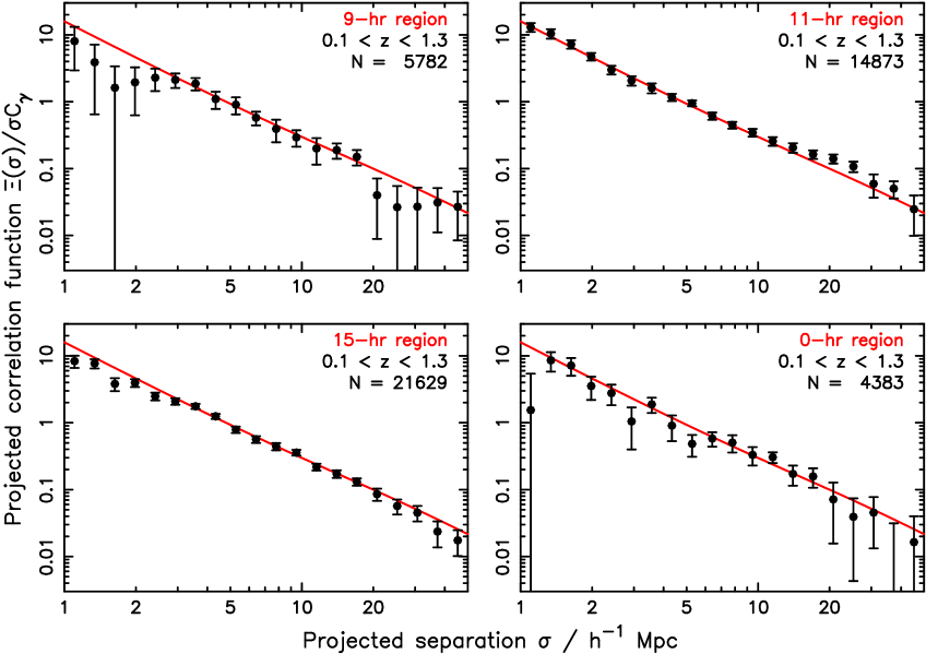
In Figure 10 we plot the separate projected correlation function measurements for each of the four survey regions analyzed in this paper. The four regions give consistent results.

Figure 10: The projected correlation function $\Xi(\sigma)/\sigma C_{\gamma}$ as a function of projected separation $\sigma$ for galaxies in the redshift range $0.1<z<1.3$, measured for the four survey regions analyzed in this paper. The solid line indicates the best-fitting power law for the whole sample, and the number of redshifts $N$ used for each region is displayed. The $y$-axis is normalized by a factor which produces numerical results approximating $(r_{0}/\sigma)^{\gamma}$.

In order to derive the bias factor of the galaxies with respect to dark matter we generated a model non-linear matter power spectrum at $z=0$ assuming a flat cosmological model with fiducial parameters $\Omega_{\rm m}=0.3$, $\Omega_{\rm b}/\Omega_{\rm m}=0.15$, $h=0.7$ (where $H_{0}=100\,h$ km s^-1 Mpc^-1) and $\sigma_{8}=0.9$, using the “CAMB” software package (Lewis, Challinor & Lasenby 2000) including corrections for non-linear growth of structure using the fitting formula of Smith et al. (2003). We used this model power spectrum to determine the non-linear matter correlation function $\xi_{\rm DM}$ at $z=0$. The resulting correlation function satisfied $\xi_{\rm DM}(r)=1$ for $r=4.7\,h^{-1}$ Mpc, which we assumed as our estimate of $r_{0,\rm{DM}}(0)$, the clustering length of dark matter at $z=0$. Given that the overall amplitude of the power spectrum scales with redshift in the linear regime as $D(z)^{2}$, where $D(z)$ is the linear growth factor, we can approximate:

$$r_{0,\rm{DM}}(z)\approx(4.7\,h^{-1}\,{\rm Mpc})\times D(z)^{2/\gamma}$$ (16)

where $\gamma\approx 1.8$. Hence the linear bias factor $b$ of a population of galaxies with clustering length $r_{0}$ can be approximated as:

$$b\approx\left(\frac{r_{0}}{r_{0,\rm{DM}}}\right)^{\gamma/2}=\left(\frac{r_{0}}{4.7\,h^{-1}\,{\rm Mpc}}\right)^{\gamma/2}\times D(z)^{-1}$$ (17)

Our measured clustering length $r_{0}=4.4\,h^{-1}$ Mpc for a sample at median redshift $z\approx 0.6$ is hence equivalent to a linear bias factor $b\approx 1.3$.

4.3 Redshift-space distortions

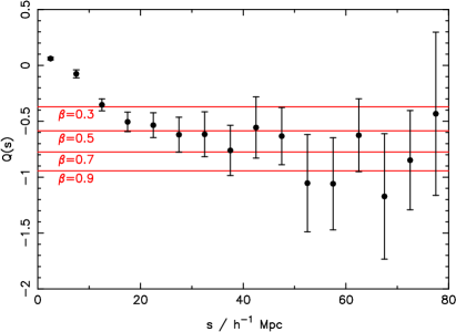
The peculiar velocities generated by large-scale coherent infall can be parameterized by $\beta\approx\Omega_{\rm m}(z)^{0.55}/b$ where $b$ is the linear bias parameter (Kaiser 1987). For a flat cosmological constant model with $\Omega_{\rm m}(0)=0.3$, $\Omega_{\rm m}(z=0.6)=0.64$, and our real-space clustering measurement $b=1.3$ hence predicts $\beta=0.6$ at the median redshift of the sample. The purpose of this Section is to demonstrate that our data contains this self-consistent signal of peculiar velocities (we leave detailed fits for $\beta$ to a further study).

We may quantify the imprint of peculiar velocities by measuring the quadrupole moment, $Q(s)$, of the 2D correlation function (Hamilton 1992). This statistic quantifies the anisotropy evident in Figure 7. If we define the correlation function moment $\xi_{\ell}$ for multipole $\ell$ as:

$$\xi_{\ell}(s)=\frac{2\ell+1}{2}\int_{-1}^{+1}\xi_{z}(s,\mu)\,P_{\ell}(\mu)\,d\mu$$ (18)

we can then show that

$$Q(s)=\frac{\xi_{2}(s)}{\left[\frac{3}{s^{3}}\int_{0}^{s}\xi_{0}(x)\,x^{2}\,dx\right]-\xi_{0}(s)}=\frac{\frac{4}{3}\beta+\frac{4}{7}\beta}{1+\frac{2}{3}\beta+\frac{1}{5}\beta^{2}}$$ (19)

which is valid for large scales $s>10\,h^{-1}$ Mpc. Figure 11 plots the measured quantity $Q(s)$ as a function of separation $s$, together with the prediction of equation 19 for various values of $\beta$. In order to construct the quantity $Q(s)$ we measured the 2D redshift-space correlation function in bins of $s$ and $\mu$, and summed over $\mu$, weighting in accordance with equation 18. The result is consistent with our estimate $\beta\approx 0.6$ and constitutes a statistically-significant detection of redshift-space distortions in our sample.

Figure 11: The statistic $Q(s)$, which encodes the anisotropy in the 2D correlation function $\xi(\sigma,\pi)$ induced by redshift-space distortions. The prediction of linear-theory on large-scales $s>10\,h^{-1}$ Mpc is indicated as a function of the parameter $\beta$.

4.4 Redshift and luminosity dependence

Our sample of WiggleZ galaxies is large enough for us to analyze the dependence of the clustering length $r_{0}$ on redshift, galaxy luminosity and colour. The situation is complicated by our joint UV-optical selection and strong luminosity-redshift correlation, but we can make some comparisons with previous studies. We fix the correlation function slope $\gamma=1.8$ in this section of the analysis.

The variation of the clustering length with redshift is plotted in Figure 12, dividing all WiggleZ galaxies in the range $0.1<z<1.0$ into redshift bins of width $\Delta z=0.1$. The clustering length is roughly constant with redshift for the range $z>0.3$, with a trend to a reduced clustering strength at low redshifts. Our interpretation of the overall constancy of $r_{0}(z)$ is that it is a product of two cancelling effects. Galaxy luminosity increases with redshift, which would tend to increase clustering length, but at redshifts $z>0.5$ optically red galaxies, which possess enhanced clustering strengths, are removed from the sample by the optical colour cuts described in Section 2.2.

Figure 12: Dependence of the best-fitting clustering length $r_{0}$ on redshift for a fit of the power-law $(r_{0}/r)^{1.8}$ to the real-space projected correlation function.

We also analyzed the clustering in absolute magnitude and rest-frame colour bins. We considered the clustering as a function of rest-frame $FUV$-band and $B$-band absolute magnitudes, which are well-matched in wavelength (for redshift $z\approx 0.5$) to the observed-frame $NUV$-band and $r$-band magnitudes which are used to define our target samples. For this initial analysis we assumed redshift-dependent average K-corrections which we applied to all galaxies regardless of colour. These K-corrections were derived using the spectral energy distribution of a Lyman Break Galaxy including an intrinsic dust contribution $A_{V}=0.14$, which produces a very good match to the redshift-dependence of the average observed $NUV-r$ colour of the WiggleZ targets.

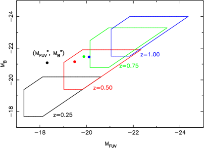
We note that the $FUV$-band and $B$-band absolute magnitudes of our target sample correlate strongly with redshift. This is depicted by Figure 13 which plots the target selection box in $(M_{FUV},M_{B})$ for 4 different redshifts, also indicating the characteristic absolute magnitudes $(M_{FUV}^{*},M_{B}^{*})$ at each redshift obtained from Arnouts et al. (2005) and Willmer et al. (2006). Between $z=0.25$ and $z=1$ the average value of $M_{FUV}-M_{FUV}^{*}$ brightens by 2 magnitudes (becoming positive at $z\approx 0.5$) and the average value of $M_{B}-M_{B}^{*}$ brightens by 4 magnitudes (becoming positive at $z\approx 0.7$).

Figure 13: The WiggleZ UV-optical target selection box in the space of $B$-band absolute magnitude $M_{B}$ and $FUV$-band absolute magnitude $M_{FUV}$ for 4 different redshifts between $z=0.25$ and $z=1$ (moving from left to right in the Figure). These absolute magnitude limits are implied by our apparent magnitude and colour selections $NUV<22.8$, $20<r<22.5$ and $-0.5<NUV-r<2$. The values of $M_{B}^{*}$ and $M_{FUV}^{*}$ at each redshift are shown for comparison (taken from Willmer et al. 2005 and Arnouts et al. 2005). Absolute magnitudes are calculated assuming $h=0.7$.

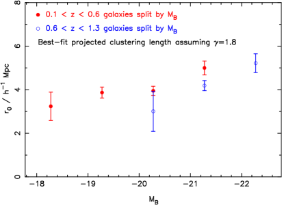
The dependence of the clustering length $r_{0}$ of the $0.1<z<1.3$ WiggleZ sample on $M_{B}$, $M_{FUV}$ and $M_{FUV}-M_{B}$ is displayed in the panels of Figure 14. These measurements show that the clustering strength of the sample increases steadily with $B$-band absolute magnitude, $FUV$-band absolute magnitude and reddening $M_{FUV}-M_{B}$ colour. Sub-samples have values of $r_{0}$ ranging from $2\,h^{-1}$ Mpc to $5\,h^{-1}$ Mpc.

Figure 14: Dependence of the best-fitting clustering length $r_{0}$ on $B$-band absolute magnitude $M_{B}$, $FUV$-band absolute magnitude $M_{FUV}$ and rest-frame colour $M_{FUV}-M_{B}$, for a fit of the power-law $(r_{0}/r)^{1.8}$ to the real-space projected correlation function. Absolute magnitudes are calculated assuming $h=0.7$.

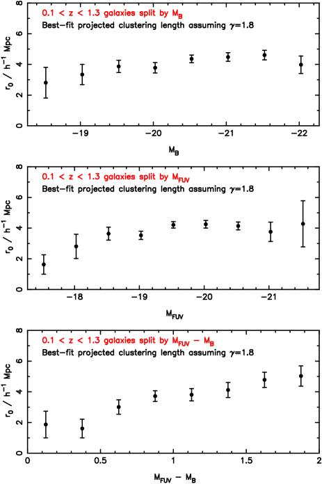
Figure 15 plots the variation of $r_{0}$ with $M_{B}$ for the low-redshift and high-redshift halves of the dataset, divided at $z=0.6$. This measurement confirms that at fixed $M_{B}$, the clustering length of the sample drops slightly with redshift as the redder galaxies are removed by the colour cuts.

Figure 15: Dependence of the best-fitting clustering length $r_{0}$ on $B$-band absolute magnitude $M_{B}$ for the upper and lower redshift ranges of our sample, for a fit of the power-law $(r_{0}/r)^{1.8}$ to the real-space projected correlation function. Absolute magnitudes are calculated assuming $h=0.7$.

4.5 Comparison to previous studies

Coil et al. (2008) present clustering measurements as a function of galaxy colour and luminosity for the DEEP2 Galaxy Redshift Survey, which has measured redshifts for $\approx 30{,}000$ galaxies in the range $0.7<z<1.5$ over an area of 3 deg². The DEEP2 subset of luminous blue galaxies (Coil et al. Table 2, line 5) has best-fitting clustering parameters $r_{0}=(4.27\pm 0.43)\,h^{-1}$ Mpc and $\gamma=1.75\pm 0.13$ at $z=1$ (for a galaxy density $n=6\times 10^{-4}\,h^{3}$ Mpc^-3 and median absolute magnitude $M_{B}=-22.1$ assuming $h=0.7$). These results lie in good agreement with ours.

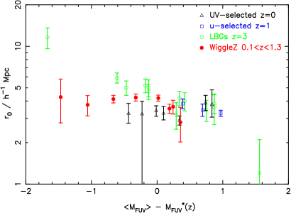
Milliard et al. (2007) and Heinis et al. (2007) present clustering analyses of GALEX-selected samples. At low redshift ($z<0.3$) the clustering strength of the UV-selected sample is $r_{0}\approx 3.5\,h^{-1}$ Mpc, corresponding to low-density environments, and shows no dependence on UV luminosity (indeed, there is tentative evidence for an anti-correlation between $r_{0}$ and luminosity). These results may naturally be compared to clustering measurements of $z\approx 3$ LBGs also selected at rest-frame UV wavelengths (e.g. Giavalisco & Dickinson 2001; Ouchi et al. 2001; Arnouts et al. 2002; Foucaud et al. 2003; Adelberger et al. 2005; Allen et al. 2005; Ouchi et al. 2005; Lee et al. 2006; Yoshida et al. 2008). These results show a qualitatively different conclusion: LBGs are highly clustered and concentrated in overdense regions. Furthermore, the clustering strength for galaxies brighter than $M_{FUV}^{*}$ increases with $FUV$ luminosity, reaching $r_{0}\approx 15\,h^{-1}$ Mpc for the most luminous sub-samples. Yoshida et al. (2008) demonstrate that the behaviour of the clustering length $r_{0}$ depends on a combination of UV and optical luminosities: galaxies bright in optical magnitudes are strongly clustered irrespective of UV magnitude, whereas galaxies faint in optical magnitude have correlation lengths increasing with UV luminosity (see Yoshida et al. Fig.15).

In Figure 16 we overplot the clustering measurements of the $0.1<z<1.3$ WiggleZ sample as a function of $FUV$ absolute magnitude on the compilation of low-redshift and high-redshift clustering measurements presented by Heinis et al. (2007). At low $FUV$ absolute magnitudes $M_{FUV}-M_{FUV}^{*}>0.5$ the clustering strengths of the different UV-selected samples agree well. This absolute magnitude range corresponds to low redshifts $z<0.3$ in the WiggleZ sample (Figure 13) for which we recover a clustering length $r_{0}\approx 3\,h^{-1}$ Mpc, similar to samples of low-redshift quiescent star-forming galaxies. At higher $FUV$ luminosities and redshifts, the WiggleZ clustering strength is more comparable to $z=3$ LBGs rather than $z=0$ UV-selected galaxies. This is expected as the $FUV-NUV$ WiggleZ selection cut becomes effective for $z>0.3$ and the nature of the resulting WiggleZ galaxy population changes to merger-induced starbursts. The WiggleZ sample does not recover the very high values of $r_{0}$ present in very luminous LBGs at $z=3$; we suggest that this may be a result of the WiggleZ colour cuts selecting against redder galaxies.

Figure 16: Comparison of the clustering segregation with FUV absolute magnitude observed in the WiggleZ sample with the compilation of low-redshift and high-redshift results presented by Heinis et al. (2007). The WiggleZ targets are more comparable to $z=3$ LBGs rather than $z=0$ UV-selected galaxies. The displayed data points are obtained from Giavalisco & Dickinson (2001), Arnouts et al. (2002), Foucaud et al. (2003), Heinis et al. (2004), Adelberger et al. (2005) and Heinis et al. (2007). Absolute magnitudes are calculated assuming $h=0.7$.

5 Forecasts for WiggleZ survey

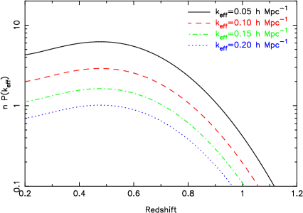
The clustering amplitude of the WiggleZ target sample is a required input for forecasting the accuracy with which the full 1000 deg² survey will measure the large-scale galaxy power spectrum. The error in the power spectrum measurement $\delta P_{\rm gal}$ at a given redshift $z$ and Fourier wavenumber $k$ is determined by the quantity $n\times P_{\rm gal}$, where $n(z)$ is the galaxy number density and $P_{\rm gal}(k,z)$ is the galaxy power spectrum amplitude. This quantity fixes the balance between sample variance and shot noise in the measurement error such that

$$\frac{\delta P_{\rm gal}}{P_{\rm gal}}=\frac{1}{\sqrt{m}}\left(1+\frac{1}{n\,P_{\rm gal}}\right)$$ (20)

where $m$ is the total number of independent Fourier modes contributing towards the measurement (e.g. Feldman, Kaiser & Peacock 1994; Tegmark 1997). The contributions of sample variance and shot noise are equal when $n\times P_{\rm gal}=1$. We model the angle-averaged redshift-space linear galaxy power spectrum as a function of $k$ and $z$ as:

$$P_{\rm gal}(k,z)=P_{\rm DM}(k,0)\left[\frac{r_{0,{\rm gal}}(z)}{r_{0,{\rm DM}}(0)}\right]^{\gamma}\left(1+\frac{2\beta}{3}+\frac{\beta^{2}}{5}\right)$$ (21)

where we assume $r_{0,{\rm DM}}(0)=4.7\,h^{-1}$ Mpc, $r_{0,{\rm gal}}(z)=4.4\,h^{-1}$ Mpc, $\gamma=1.9$ and $\beta=0.6$. The second term on the right-hand-side of equation 21 describes the boost from the galaxy linear bias factor $b$ (equation 17) using the relation $P_{\rm gal}=P_{\rm DM}b^{2}D^{2}$. The third term is the result of redshift-space distortions averaged over angles. We used the cosmological parameters as listed in Section 4.2 to produce the $z=0$ dark matter power spectrum: $\Omega_{\rm m}=0.3$, $\Omega_{\rm b}/\Omega_{\rm m}=0.15$, $h=0.7$ and $\sigma_{8}=0.9$. In order to incorporate the fraction of redshift blunders $f_{\rm bad}$ we reduced the effective value of the power spectrum by a factor $(1-f_{\rm bad})^{2}$ [i.e. increased the value of $r_{0,{\rm DM}}(0)$ by a factor $(1-f_{\rm bad})^{-2/\gamma}$].

Figure 17 plots the dependence of $n\times P_{\rm gal}$ on redshift for a set of different scales $0.05<k<0.2\,h$ Mpc^-1 relevant for the detection of baryon acoustic oscillations, assuming a source redshift distribution combining the survey regions plotted in Figure 2. We further assume a total target density of 350 deg^-2 with a $70\%$ redshift completeness. We note that over a significant range of redshifts and scales our large-scale power spectrum measurement will be limited by sample variance rather than shot noise, i.e. $n\times P_{\rm gal}>1$.

A useful quantity to describe the survey is the scale-dependent “effective volume” $V_{\rm eff}(k)$ which is defined by

$$V_{\rm eff}(k)=\int_{0}^{\infty}\left[\frac{n(z)P_{\rm gal}(k,z)}{1+n(z)P_{\rm gal}(k,z)}\right]^{2}\frac{dV}{dz}\,dz$$ (22)

where $dV/dz$ is the co-moving volume element. The effective volume represents an optimally-weighted stacking of power spectrum measurements at different redshifts (Tegmark 1997). For scales $k=(0.05,0.1,0.15,0.2)\,h$ Mpc^-1 we find $V_{\rm eff}=(0.65,0.41,0.25,0.15)\,h^{-3}$ Gpc³. Thus the survey design will achieve the goal of mapping $\sim 1$ Gpc${}^{3}=0.34\,h^{-3}$ Gpc³.

Figure 17: The dependence of $n\times P_{\rm gal}$ on redshift for four scales $k$ representative of those important for the measurement of baryon acoustic oscillations. If $n\times P_{\rm gal}=1$, then the contribution of shot noise to the power spectrum error equals that of sample variance.

We can use the effective survey volume to forecast the error in the final survey power spectrum $\delta P_{\rm gal}(k)$ in a Fourier bin of width $\Delta k$ (Tegmark 1997):

$$\frac{\delta P_{\rm gal}}{P_{\rm gal}}=\frac{2\pi}{k\sqrt{V_{\rm eff}(k)\,\Delta k}}$$ (23)

This prediction is plotted for bins of width $\Delta k=0.01\,h$ Mpc^-1 in Figure 18, in which we divide the power spectrum by the “no-wiggles” reference spectrum provided by Eisenstein & Hu (1998) in order to delineate clearly the baryon acoustic oscillations.

Figure 18: Simulation of the errors in the final WiggleZ survey galaxy power spectrum. We have divided by a smooth “reference” power spectrum to clarify the signature of baryon acoustic oscillations.

We also generated 100 Monte Carlo realizations of the final 1000 deg² survey using the methods described in Blake & Glazebrook (2003) and Glazebrook & Blake (2005). The scatter in the power spectrum measurements across the realizations was very close to that predicted by equation 23. We used these Monte Carlo realizations to assess the accuracy with which the full WiggleZ survey will measure the tangential and radial standard ruler scale imprinted by the baryon acoustic oscillations via the fitting formula described in Blake et al. (2006). Restricting ourselves to the $0.3<z<0.9$ subset, and first considering an “angle-averaged” measured power spectrum $P(k)$, we found that the scatter in the fitted acoustic wavescale was $2.8\%$. Measuring instead a 2D power spectrum $P(k_{\rm tan},k_{\rm rad})$, where $k_{\rm tan}$ and $k_{\rm rad}$ are wavevectors measured perpendicular and parallel to the line-of-sight, the scatters in the tangential and radial fitted wavescales were $4.6\%$ and $7.2\%$, respectively. This latter pair of measurements corresponds to the accuracy of determination of the quantities $D_{A}(z)/s$ and $H(z)^{-1}/s$ at an effective redshift $z\approx 0.6$, where $D_{A}$ is the angular diameter distance, $H(z)$ is the high-redshift Hubble constant, and $s$ is the sound horizon at recombination, i.e. the standard ruler scale. Dividing the survey into redshift slices we find that the angle-averaged wavescale may be measured with accuracy $(6.6\%,3.7\%,6.3\%)$ in redshift slices $(0.25-0.5,0.5-0.75,0.75-1)$. The angle-averaged wavescale measures a quantity proportional to $(D_{A}^{2}H^{-1})^{1/3}$, as discussed by Eisenstein et al. (2005).

These forecasts should be considered a pessimistic lower limit on expected performance for two reasons. Firstly we have neglected the cosmological information contained in the overall shape of the galaxy power spectrum, which is divided out in the above analysis to focus on the “standard ruler” aspect of the acoustic oscillations. This method produces robustness against systematic errors (which are expected to affect the shape of the power spectrum but not the oscillatory signature). The power spectrum shape carries information about $\Omega_{\rm m}$ and $H_{0}$ which further breaks the degeneracy in cosmological distances between these two parameters and the dark energy. Secondly we have neglected the improvement offered by “reconstruction” of the density field, which sharpens the measurement of the acoustic signature by un-doing (to first order) the large-scale coherent galaxy motions which smooth out the acoustic peaks (Eisenstein et al. 2007).

Table 1: Model WiggleZ survey parameters in one and three redshift bins used to forecast cosmological parameter measurements. The bias factor has been multiplied by a factor $1-f_{\rm bad}$ to produce an effective value allowing for the redshift blunder rate. The five standard ruler accuracies acc₁, acc₂, acc₃, acc₄, acc₅ are respectively the tangential and radial precision predicted by the Blake et al. (2006) fitting formula, an angle-averaged version of the Blake et al. formula, and the tangential and radial accuracies predicted by the Seo & Eisenstein (2007) fitting formula including density reconstruction. In the Blake et al. formula the effective bias is increased by a factor $\sqrt{1+\frac{2}{3}\beta+\frac{1}{5}\beta^{2}}=1.21$ to allow for redshift-space effects. Further details are given in the text.

Redshift slice	Number density	$r_{0,{\rm gal}}$	Bias factor	Blunder rate	acc1	acc2	acc3	acc4	acc5
	($\times 10^{-4}\,h^{3}$ Mpc-3)	$h^{-1}$ Mpc	$b$	$f_{\rm bad}$	(%)	(%)	(%)	(%)	(%)
$0.3<z<0.9$	2.29	4.3	1.21	0.037	4.6	7.2	2.8	2.7	4.3
$0.25<z<0.5$	3.33	4.0	1.01	0.038	-	-	6.6	5.5	8.7
$0.5<z<0.75$	2.78	4.4	1.27	0.022	-	-	3.7	3.6	5.8
$0.75<z<1$	0.83	4.4	1.27	0.127	-	-	6.3	7.9	10.9

We investigated improved forecasts using the methodology of Seo & Eisenstein (2007) which properly incorporates information from the power spectrum shape, redshift-space distortions and density-field reconstruction. The predicted tangential and radial measurement accuracies for the $0.3<z<0.9$ sample are $2.7\%$ and $4.3\%$, respectively (and are correlated with a correlation coefficient $r\approx 0.4$, further enhancing the power to constrain the cosmological model). We assume here that reconstruction can improve the parameters ($\Sigma_{\perp}$, $\Sigma_{\parallel}$) defined by Seo & Eisenstein (2007) by a factor equal to $0.5-0.3\,{\rm log}_{10}(n\times P_{\rm gal})$ (Eisenstein, priv. comm.). Dividing the survey into redshift slices we find that the tangential and radial wavescales may be measured with accuracies $(5.5\%,8.7\%)$ for $0.25<z<0.5$, $(3.6\%,5.8\%)$ for $0.5<z<0.75$ and $(7.9\%,10.9\%)$ for $0.75<z<1$. This information is collected in Table 1 for ease of reference.

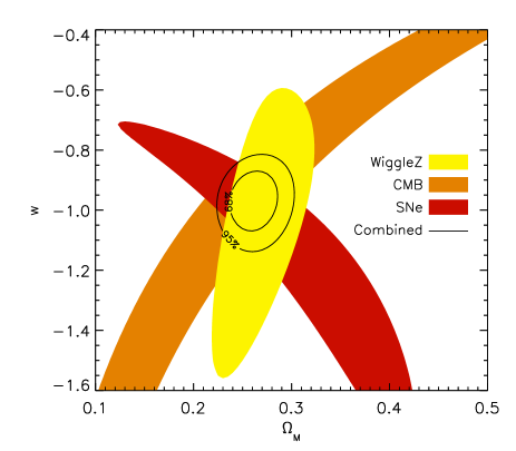
We used this last set of forecasts with reconstruction in 3 redshift bins to determine the expected accuracy of measurement of a constant equation-of-state $w_{\rm cons}$ of dark energy (assuming the measurements of $D_{A}$ and $H^{-1}$ are correlated with coefficient $r=0.4$). Confidence ellipses are displayed in Figure 19 in the space of $w_{\rm cons}$ and the matter density $\Omega_{\rm m}$ for a flat cosmology with fiducial model $w_{\rm cons}=-1$ and $\Omega_{\rm m}=0.27$. Results are shown for each redshift bin separately and for the combination of all 3 bins. In order to generate this Figure we have used the 5-year-WMAP measurement of the CMB acoustic scale $\ell_{A}=302.1\pm 0.9$ (Komatsu et al. 2009) in order to cancel the dependence of the baryon oscillation measurement on the sound horizon at recombination. In Figure 19 we have not included any further CMB information or other external datasets. The marginalized errors are $\sigma(w_{\rm cons})=0.31$ and $\sigma(\Omega_{\rm m})=0.03$.

Figure 19: The forecast $68\%$ confidence ellipses for measurements of a constant dark energy equation-of-state $w_{\rm cons}$ and the matter density $\Omega_{\rm m}$ using standard ruler measurements from the final WiggleZ survey in combination with a CMB prior on the acoustic scale $\ell_{A}$. Results are shown for 3 redshift bins (the different contours) and for the combination of the redshift bins (the shaded area).

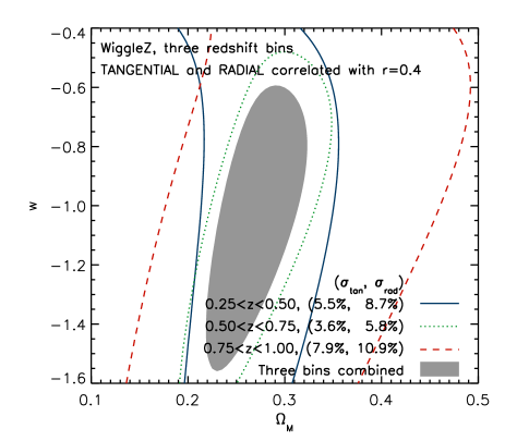
In Figure 20 we add in information from the 5-year-WMAP measurement of the CMB shift parameter $R=1.71\pm 0.02$ (Komatsu et al. 2009), including the correlation between $R$ and $\ell_{A}$, together with the latest supernovae data from the Essence, SNLS and HST observations (see Wood-Vasey et al. 2007, Astier et al. 2006, Riess et al. 2007, Davis et al. 2007). The marginalized errors in the cosmological model from the full combination of datasets are $\sigma(w_{\rm cons})=0.07$ and $\sigma(\Omega_{\rm m})=0.02$. The forecast performance of the WiggleZ survey exceeds that of the current CMB and supernovae data, but the different measurements are also complementary, breaking degeneracies in the $(\Omega_{\rm m},w_{\rm cons})$-plane through independent techniques. Disagreement between any pair of datasets would produce the possibility of discovering non-standard physics (if it exists) or systematic measurement errors. The final accuracy of $w_{\rm cons}$ constitutes a robust and precise test of the dark energy model.

Figure 20: The forecast $68\%$ confidence ellipse for measurement of $(\Omega_{\rm m},w_{\rm cons})$ from the WiggleZ survey plus CMB acoustic scale (the yellow ellipse), compared with existing measurements from the CMB shift parameter (the orange ellipse) and latest supernovae (the red ellipse). The $68\%$ and $95\%$ confidence regions for the combination of all the datasets is displayed as the central contours.

6 Conclusions

We have measured the small-scale clustering amplitude of high-redshift bright emission-line galaxies using the first $20\%$ of spectra from the AAT WiggleZ Dark Energy Survey ($\approx 47{,}000$ galaxies in the redshift range $0.1<z<1.3$). We have successfully developed a methodology to generate random realizations of the survey incorporating the currently sparse selection function and redshift incompleteness. We find that:

• The WiggleZ galaxy sample in the redshift range $0.1<z<1.3$ possesses a clustering length $r_{0}=4.40\pm 0.12\,h^{-1}$ Mpc and slope $\gamma=1.92\pm 0.08$. This clustering amplitude significantly exceeds that of UV-selected samples at $z\approx 0$ and agrees well with that of the most luminous blue galaxies observed by the DEEP2 galaxy redshift survey at $z\approx 1$. The clustering amplitude of WiggleZ targets is comparable to that of Lyman Break Galaxies at a similar UV luminosity.

• The clustering length of the WiggleZ targets is approximately constant with redshift for the range $z>0.3$. The value of $r_{0}$ increases with $B$-band luminosity, $FUV$-band luminosity, and reddening rest-frame colour.

• The redshift-space distortion signature of coherent galaxy motions is detected and its amplitude ($\beta\approx 0.6$) is consistent with that predicted from the galaxy bias. We detect some evidence for “fingers of god” due to the virialized motions of galaxies in clusters.

Using these results, we forecast the performance of the full 1000 deg² WiggleZ survey in the measurement of the galaxy power spectrum and cosmological model. We find that:

• The survey design is well-tuned to the “optimal” mean galaxy number density $n\sim P_{\rm gal}^{-1}$, where $P_{\rm gal}$ is the amplitude of the galaxy power spectrum on the scales of importance for baryon oscillations.

• The survey will delineate the baryon acoustic oscillations in the large-scale clustering pattern in three independent redshift slices, providing measurements of the cosmic distance and expansion rate in each redshift slice with accuracies of $\approx 5\%$.

• The resulting measurement of a constant dark energy equation-of-state parameter $w_{\rm cons}$ from the WiggleZ survey, calibrating the standard ruler using the CMB measurement of the acoustic scale, has a higher precision than provided by current supernovae datasets. These independent dark energy probes lie in a highly complementary direction in the parameter space of $w_{\rm cons}$ and $\Omega_{\rm m}$. The full combination of WiggleZ, supernovae and CMB datasets provides a measurement of the equation of state with accuracy $\Delta w_{\rm cons}=0.07$, constituting a robust and precise test of the dark energy model incorporating cross-checking of systematic errors between different probes.

The final survey will enable a wide range of scientific investigations into the cosmological model and galaxy evolution.

References

- [1] Adelberger K.L., Steidel C.C., Pettini M., Shapley A.E., Reddy N.A., Erb D.K., 2005, ApJ, 619, 697
- [2] Allen P.D., Moustakas L.A., Dalton G., MacDonald E., Blake C.A, Clewley L., Heymans C., Wegner G., 2005, MNRAS, 360, 1244
- [3] Arnouts S. et al., 2002, MNRAS, 329, 355
- [4] Arnouts S. et al., 2005, ApJ, 619, 43
- [5] Astier P. et al., 2006, A&A, 447, 31
- [6] Blake C.A, Glazebrook K., 2003, ApJ, 594, 665
- [7] Blake C.A., Parkinson D., Bassett B., Glazebrook K., Kunz M., Nichol R.C., 2006, MNRAS, 365, 255
- [8] Campbell L., Saunders W., Colless M., 2004, MNRAS, 350, 1467
- [9] Coil A. et al., 2008, ApJ, 672, 153
- [10] Cole S. et al., 2005, MNRAS, 362, 505
- [11] Coles P., 1993, MNRAS, 262, 1065
- [12] Colless M. et al., 2001, MNRAS, 328, 1039
- [13] Cowie L.L., Songaila A., Hu E.M., Cohen J.G., 1996, AJ, 112, 839
- [14] Cooray A., Hu W., Huterer D., Joffre M., 2001, ApJ, 557L, 7
- [15] Davis M., Peebles P.J.E., 1983, ApJ, 208, 13
- [16] Davis T.M. et al., 2007, ApJ, 666, 716
- [17] Efstathiou G., 1988, in Lawrence A., ed., Proc. 3rd IRAS Conf., Comets to Cosmology, Springer, New York, p.312
- [18] Eisenstein D.J., Hu W., 1998, ApJ, 518, 2
- [19] Eisenstein D.J. et al., 2001, AJ, 122, 2267
- [20] Eisenstein D.J., 2002, ‘Large-scale structure and future surveys’ in ‘Next Generation Wide-Field Multi-Object Spectroscopy’, ASP Conference Series vol. 280, ed. M.Brown & A.Dey, p.35 (astro-ph/0301623)
- [21] Eisenstein D.J. et al., 2005, ApJ, 633, 560
- [22] Eisenstein D.J., Seo H.-J., Sirko E., Spergel D.N., 2007, ApJ, 664, 675
- [23] Feldman H.A., Kaiser N., Peacock J.A., 1994, ApJ, 426, 23
- [24] Foucaud S., McCracken H.J., Le Fevre O., Arnouts S., Brodwin M., Lilly S.J., Crampton D., Mellier Y., 2003, A&A, 409, 835
- [25] Gaztanaga E., Cabre A., Hui L., 2008, submitted (astro-ph/0807.3551)
- [26] Giavalisco M., Dickinson M., 2001, ApJ, 550, 177
- [27] Glazebrook K. et al., 2004, Nature, 430, 181
- [28] Glazebrook K., Blake C.A., 2005, ApJ, 631, 1
- [29] Hamilton A.J.S., 1992, ApJ, 385, 5
- [30] Hawkins E. et al., 2003, MNRAS, 346, 78
- [31] Heinis S., Treyer M., Arnouts S., Milliard B., Donas J., Gal R., Martin D.C., Viton M., 2004, A&A, 424, L9
- [32] Heinis S. et al., 2007, ApJS, 173, 503
- [33] Hu W., Haiman Z., 2003, Phys. Rev. D, 68, 063004
- [34] Huesti G., 2006, A&A, 449, 891
- [35] Kaiser N., 1987, MNRAS, 227, 1
- [36] Komatsu E. et al., 2009, ApJS, 180, 330
- [37] Landy S.D., Szalay A.S., 1993, ApJ, 412, 64
- [38] Lee K.-S., Giavalisco M., Gnedin O., Somerville R.S., Ferguson H.C., Dickinson M., Ouchi M., 2006, ApJ, 642, 63
- [39] Lewis A., Challinor A., Lasenby A., 2000, ApJ, 538, 473
- [40] Linder E.V., 2003, Phys. Rev. D, 68, 083504
- [41] Loveday J., Maddox S.J., Efstathiou G., Peterson B.A., 1995, ApJ, 442, 457
- [42] Martin D., et al., 2005, ApJ, 619, L1
- [43] Meneux B. et al., 2006, A&A, 452, 387
- [44] Milliard B. et al., 2007, ApJS, 173, 494
- [45] Ouchi M. et al., 2001, ApJ, 558, L83
- [46] Ouchi M. et al., 2005, ApJ, 635, L117
- [47] Parkinson D., Blake C.A., Kunz M., Bassett B., Nichol R., Glazebrook K., 2007, MNRAS, 377, 185
- [48] Percival W., Cole S., Eisenstein D.J., Nichol R.C., Peacock J.A., Pope A.C., Szalay A.S., 2007, MNRAS, 381, 1053
- [49] Riess A. et al., 2007, ApJ, 659, 98
- [50] Saunders W. et al., 2004, ‘AAOmega: a scientific and optical overview’ in ‘Ground-based Instrumentation for Astronomy’, ed. A.Moorwood & I.Masanori, Proceedings of the SPIE, vol. 5492, p.389
- [51] Scherrer R.J., Weinberg D.H., 1998, ApJ, 504, 607
- [52] Schlegel D.J., Finkbeiner D.P., Davis M., 1998, ApJ, 500, 525
- [53] Sharp R. et al., 2006, ‘Performance of AAOmega: the AAT multi-purpose fiber-fed spectrograph’ in ‘Ground-based and Airborne Instrumentation for Astronomy’, ed. I.McLean & I.Masanori, Proceedings of the SPIE, vol. 6269, p.14 (astro-ph/0606137)
- [54] Seo H.-J., Eisenstein D.J., 2003, ApJ, 598, 720
- [55] Seo H.-J., Eisenstein D.J., 2007, ApJ, 665, 14
- [56] Smith R.E. et al., 2003, MNRAS, 341, 1311
- [57] Tegmark M., 1997, PRL, 79, 20
- [58] van Dokkum P. et al., 2004, ApJ, 611, 703
- [59] Willmer C. et al., 2006, ApJ, 647, 853
- [60] Wood-Vasey W. et al., 2007, ApJ, 666, 694
- [61] Yee H., Gladders M., Gilbank D., Majumdar S., Hoekstra H., Ellingson E., 2007, ‘The Red-Sequence Cluster Surveys’ in ‘Cosmic Frontiers ASP Conference Series’, ed. N.Metcalfe & T.Shanks, vol. 379, p.103 (astro-ph/0701839)
- [62] York D.G. et al., 2000, AJ, 120, 1579
- [63] Yoshida M., Shimasaku K., Ouchi M., Sekiguchi K., Furuswawa H., Okamura S., 2008, ApJ, 679, 269