-

Scuola di Dottorato “Vito Volterra”
Dottorato di Ricerca in Fisica
Weak Response of Nuclear Matter
Thesis submitted to obtain the degree of
“Dottore di Ricerca” – Philosophiæ Doctor
PhD in Physics – XXI cycle – October 2008
by
Nicola Farina
Program Coordinator Thesis Advisor Prof. Enzo Marinari Dr. Omar Benhar    

Introduction

The description of neutrino interactions with nuclei, and nuclear matter in general, is relevant to the study of many different problems, from supernov$\ae$ explosions to neutron star cooling, as well as to the determination of the properties of neutrino itself, most notably its mass.

The appearance of a supernova is the last stage of the evolution of stars with initial mass bigger than $\sim$ 4 $M_{\odot}$, where $M_{\odot}\approx$ 2 $\times 10^{33}$ g denotes the solar mass [1, 2, 3]. Although the first attempts to simulate a supernova explosion date more than 30 years back [4], the problem is not solved yet. In fact, the results of numerical calculations predict that, due to loss of energy carried away by neutrinos, produced in the dissociation of atomic nuclei in the core, the explosion does not occur.

The systematic uncertainty associated to simulations depends heavily on the values of the neutrino-nucleon and neutrino-nucleus reaction rates used as inputs. As many existing programs use values obtained from models based on somewhat oversimplified nuclear dynamics [5, 6, 7], such uncertainty may be significantly reduced adopting more realistic models, which have proved very successfull in the description of electro-magnetic interaction of nuclei (see, e.g., Refs. [8, 9]).

A similar problem arises in the field of neutrino physics, which is rapidly developing after the discovery of atmospheric and solar neutrino oscillation [10, 11, 12]. The experimental results point to two very distinct mass differences , $\Delta m^{2}_{sol}\approx 8.2\times 10^{-5}$ eV² and $|\Delta m^{2}_{atm}|\approx 2.5\times 10^{-3}$ eV². Only two out of the four parameters of the three-family leptonic mixing matrix $U_{PMNS}$ are known: $\theta_{12}\approx 34^{\circ}$ and $\theta_{23}\approx 45^{\circ}$. The other two parameters, $\theta_{13}$ and $\delta$, are still unknown: for the mixing angle $\theta_{13}$ direct searches at reactors [15] and three-family global analysis of the experimental data [16, 17] give the upper bound $\theta_{13}\leq 11.5^{\circ}$, whereas for the leptonic CP-violating phase $\delta$ we have no information whatsoever. Two additional discrete unknowns are the sign of the atmospheric mass difference and the $\theta_{23}$-octant.

Neutrino oscillation experiments measure energy and emission angle of the charged leptons produced in neutrino-nucleus interactions, and use the obtained results to reconstruct the incoming neutrino energy. Hence, the quantitative understanding of the neutrino-nucleus cross section, as well as of the energy spectra and angular distribution of the final state leptons, is critical to reduce the systematic uncertainty of data analysis. A number of theoretical studies aimed at providing accurate predictions of neutrino-nucleus scattering observables are discussed in Refs. [18, 19, 20].

It is important to realize that, while neutrinos interacting in stellar matter typically have energies of the order of few MeV, the energies involved in long baseline oscillations experiments are much larger. For example, K2K takes data in the region $E_{\nu}=0.5-3$ GeV.

The huge difference in kinematical conditions is reflected by different reaction mechanisms. For neutrinos of energy $\mathrel{\hbox to0.0pt{\lower 4.0pt\hbox{\hskip 1.0pt$\sim$}\hss}\raise 1.0pt\hbox{$<$}}10$ MeV, since the spatial resolution of incoming particle is much bigger than the average distance between nucleons, the nuclear response is largely determined by many-body effects.

On the other hand, at energies of the order of 1 GeV, it is reasonable to expect that the scattering process on a nucleus reduce to the incoherent sum of elementary processes involving individual nucleons. Furthermore, in this kinematical regime one needs to take into account the fact that elementary neutrino-nucleon interactions can give rise to inelastic processes, leading to the appearance of hadrons other than protons and neutrons.

The results of electron- and hadron-induced nucleon knock-out experiments have provided overwhelming evidence of the inadequacy of the independent particle model to describe the full complexity of nuclear dynamics [22, 23]. While the peaks corresponding to knock-out from shell model orbits can be clearly identified in the measured energy spectra, the corresponding strengths turn out to be consistently and sizably lower than expected, independent of the nuclear mass number. This discrepancy is mainly due to the effect of dynamical correlations induced by the nucleon-nucleon force, whose effect is not taken into account in the independent particle model.

Nuclear many body theory provides a scheme allowing for a consistent treatment of neutrino-nucleus interactions at both high and low energies. Within this approach, nuclear dynamics is described by a phenomenological hamiltonian, whose structure is completely determined by the available data on two- and three-nucleon systems, and dynamical correlations are taken into account.

Over the past decade, the formalism based on correlated wave functions, originally proposed to describe quantum liquids [24], has been employed to carry out highly accurate calculations of the binding energies of both nuclei and nuclear matter, using either the Monte Carlo method [25, 26, 27] or the cluster expansion formalism and the Fermi Hypernetted Chain integral equations [28, 29, 30].

A different approach, recently proposed in Refs. [31, 32] exploits the correlated wave functions to construct an effective interaction suitable for use in standard perturbation theory. This scheme has been employed to obtain a variety of nuclear matter properties, including the neutrino mean free path [31] and the transport coefficients [32, 33].

In this work we describe the application of the formalism based on correlated wave functions and the effective interaction to the calculation of the weak response of atomic nuclei and uniform nuclear matter.

The Thesis is structured as follows.

In Chapter 1, we briefly describe the main features of nuclear matter and nuclear forces.

In Chapter 2, we focus on the theory of nuclear matter, introducing the correlated states and the cluster expension formalism, needed to define the effective interaction. The applicability of perturbation theory within this framework is also discussed.

Chapter 3 is devoted to an overview of the many body theory of the nuclear matter response, and its connection to the spectral function.

In Chapter 4 we discuss the assumptions underlying the impulse approximation, and its applicability in the high energy regime. After a short description of the main features of the spectral function obtained from nuclear many-body theory, we compare the calculated electron-nucleus cross sections to data, and show the predictions of our approach for charged current neutrino-nucleus interactions.

Finally, in Chapter 5 we focus on the low energy regime. We develop a formalism based on the effective interaction of Ref. [32] and an effective Fermi transition operator, obtained at the same order of the cluster expansion. The effects of both short and long range correlatios, described within the correlated Hartree Fock and Tamm-Dancoff approximations, are discussed.

Note that in this Thesis we use a system of units in which $\hbar=h/2\pi=c=1$, where $h$ is the Planck constant and $c$ is the speed of light in the vacuum.

Capitolo 1 Nuclear matter and nuclear forces

Nuclear matter can be thought of as a giant nucleus, with given numbers of protons and neutrons interacting through nuclear forces only. As the typical thermal energies are negligible compared to the nucleon Fermi energies, such a system can be safely considered to be at zero temperature.

A quantitative understanding of the properties of nuclear matter, whose calculation is greatly simplified by translational invariance, is needed both as an intermediate step towards the description of real nuclei and for the development of realistic models of matter in the neutron star core.

The large body of data on nuclear masses can be used to extract empirical information on the equilibrium properties of symmetric nuclear matter (SNM), consisting of equal numbers of protons and neutrons.

The (positive) binding energy of nuclei of mass number $A$ and electric charge $Z$, defined as

$$\frac{B({\rm Z},{\rm A})}{A}=\frac{1}{A}\left[{\rm Z}m_{p}+({\rm A}-{\rm Z})m_{n}+{\rm Z}m_{e}-M({\rm Z},{\rm A})\right]\ ,$$ (1.1)

where $M({\rm Z},{\rm A})$ is the measured nuclear mass and $m_{p}$, $m_{n}$ and $m_{e}$ denote the proton, neutron and electron mass, respectively, is almost constant for A$\geq$ 12 , its value being $\sim$ 8.5 MeV (see Fig. 1.1). The $A$-dependence is well described by the semi-empirical mass formula

$$\frac{B}{A}=\frac{1}{A}\left[\right.a_{\rm V}A-a_{\rm s}A^{2/3}-a_{\rm c}\frac{Z^{2}}{A^{1/3}}-a_{A}\frac{(A-2Z)^{2}}{4A}+\lambda\ a_{\rm p}\frac{1}{A^{1/2}}\left.\right]\ .$$ (1.2)

The first term in square brackets, proportional to A, is called the volume term and describes the bulk energy of nuclear matter. The second term, proportional to the nuclear radius squared, is associated with the surface energy, while the third one accounts for the Coulomb repulsion between Z protons uniformly distributed within a sphere of radius R. The fourth term, that goes under the name of symmetry energy is required to describe the experimental observation that stable nuclei tend to have the same number of neutrons and protons. Moreover, even-even nuclei (i.e. nuclei having even Z and even A $-$ Z) tend to be more stable than even-odd or odd-odd nuclei. This property is accounted for by the last term in the above equation, where $\lambda$ $-$1, 0 and +1 for even-even, even-odd and odd-odd nuclei, respectively. Fig. 1.1 shows the different contributions to $B({\rm Z},{\rm A})/{\rm A}$, evaluated using Eq. (1.2).

In the $A\rightarrow\infty$ limit, and neglecting the effect of Coulomb repulsion between protons, the only contribution surviving in the case $Z=A/2$ is the term linear in $A$. Hence, the coefficient $a_{V}$ can be identified with the binding energy per particle of SNM.

Figura 1.1: Upper panel: A-dependence of the binding energy per nucleon of stable nuclei, evaluated according to Eq. (1.2) with $a_{\rm V}$ = 15.67 MeV, $a_{\rm s}$ = 17.23 MeV, $a_{\rm c}$ = .714 MeV, $a_{\rm A}$ = 93.15 MeV and $a_{\rm p}$ = 11.2 MeV. Lower panel: the solid line shows the magnitude of the volume contribution to the binding energy per nucleon, whereas the A-dependence of the surface, coulomb and symmetry contributions are represented by diamonds, squares and crosses, respectively.

The equilibrium density of SNM, $\rho_{0}$, can be inferred exploiting the saturation of nuclear densities, i.e. the experimental observation that the central charge density of atomic nuclei, measured by elastic electron-nucleus scattering, does not depend upon $A$ for large $A$. This property is illustrated in Fig. 1.2.

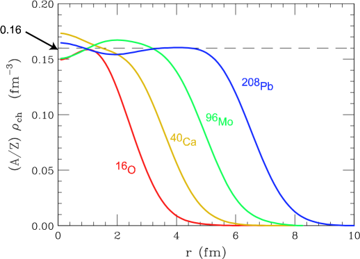
Figura 1.2: Saturation of central nuclear densities measured by elastic electron-nucleus scattering.

The empirical values of the binding energy and equilibrium density of SNM are

$$\rho_{0}=0.16\,\textrm{fm}^{-3}\ \ ,\ \ E=-15.7\,\textrm{MeV}\ .$$ (1.3)

In principle, additional information can be obtained from measurements of the excitation energies of nuclear vibrational states, yielding the (in)-compressibility module $K$. However, the data analysis of these experiments is non trivial, and the resulting values of $K$ range from $K\sim 200$ MeV (corresponding to more compressible nuclear matter, i.e. to a soft equation of state (EOS)) to $K\sim 300$ MeV (corresponding to a stiff EOS) [34].

The main goal of nuclear matter theory is deriving a EOS at zero temperature (i.e. the density dependence of the binding energy per particle $E=E(\rho)$) capable to explain the above data starting from the elementary nucleon-nucleon (NN) interaction. However, many important applications of nuclear matter theory require that its formalism be also flexible enough to describe the properties of matter at finite temperature.

Unfortunately, due to the complexity of the fundamental theory of strong interactions, the quantum chromo-dynamics (QCD), an ab initio description of nuclear matter at finite density and zero temperature is out of reach of the present computational techniques. As a consequence, one has to rely on dynamical models in which nucleons and mesons play the role of effective degrees of freedom.

In this work we adopt the approach based on nonrelativistic quantum mechanics and phenomenological nuclear hamiltonians, that allows for a quantitative description of both the two-nucleon bound state and nucleon-nucleon scattering data.

In this Chapter we outline the main features of nuclear interactions and briefly describe the structure of the NN potential models employed in many-body calculations.

1.1 Nuclear forces

The main features of the NN interaction, inferred from the analysis of nuclear systematics, may be summarized as follows.

• The saturation of nuclear density (see Fig. 1.2), i.e. the fact that density in the interior of atomic nuclei is nearly constant and independent of the mass number $A$, tells us that nucleons cannot be packed together too tightly. Hence, at short distance the NN force must be repulsive. Assuming that the interaction can be described by a nonrelativistic potential $v$ depending on the inter-particle distance, ${\bf r}$, we can then write:

  $$v({\bf r})>0\ \ \ ,\ \ |{\bf r}|<r_{c}\ ,$$ (1.4)

  $r_{c}$ being the radius of the repulsive core.

• The fact that the nuclear binding energy per nucleon is roughly the same for all nuclei with $A\geq$ 12 suggests that the NN interaction has a finite range $r_{0}$, i.e. that

  $$v({\bf r})=0\ \ \ ,\ \ |{\bf r}|>r_{0}\ .$$ (1.5)

• The spectra of the so called mirror nuclei, i.e. pairs of nuclei having the same $A$ and charges differing by one unit (implying that the number of protons in a nucleus is the same as the number of neutrons in its mirror companion), e.g. ${}^{15}_{\ 7}$N ($A$ = 15, $Z$ = 7) and ${}^{15}_{\ 8}$O ($A$ = 15, $Z$ = 8), exhibit striking similarities. The energies of the levels with the same parity and angular momentum are the same up to small electromagnetic corrections, showing that protons and neutrons have similar nuclear interactions, i.e. that nuclear forces are charge symmetric.

Charge symmetry is a manifestation of a more general property of the NN interaction, called isotopic invariance. Neglecting the small mass difference, proton and neutron can be viewed as two states of the same particle, the nucleon (N), described by the Dirac equation obtained from the Lagrangian density

$${\cal L}=\bar{\psi}_{N}\left(i\gamma^{\mu}\partial_{\mu}-m\right)\psi_{N}$$ (1.6)

where

$$\psi_{N}=\left(\begin{array}[]{c}p\\ n\end{array}\right)\ ,$$ (1.7)

$p$ and $n$ being the four-spinors associated with the proton and the neutron, respectively. The lagrangian density (1.6) is invariant under the $SU(2)$ global phase transformation

$$U={\rm e}^{i\alpha_{j}\tau_{j}}\ ,$$ (1.8)

where ${\bm{\alpha}}$ is a constant (i.e. independent of $x$) vector and the $\tau_{j}$ ($j=1,2,3$) are Pauli matrices (whose properties are briefly collected in Appendix A). The above equations show that the nucleon can be described as a doublet in isospin space. Proton and neutron correspond to isospin projections $+$1/2 and $-$1/2, respectively. Proton-proton and neutron-neutron pairs always have total isospin T=1 whereas a proton-neutron pair may have either $T=0$ or $T=1$. The two-nucleon isospin states $|T,M_{T}\rangle$ can be summarized as follows (see also Appendix A)

$$|1,1\rangle = |pp\rangle$$

$$|1,0\rangle = \frac{1}{\sqrt{2}}\left(|pn\rangle+|np\rangle\right)$$

$$|1,-1\rangle = |nn\rangle$$

$$|0,0\rangle = \frac{1}{\sqrt{2}}\left(|pn\rangle-|np\rangle\right)\ .$$

Isospin invariance implies that the interaction between two nucleons separated by a distance $r=|{\bf r}_{1}-{\bf r}_{2}|$ and having total spin $S$ depends on their total isospin $T$ but not on its projection $M_{T}$. For example, the potential $v({\bf r})$ acting between two protons with spins coupled to $S=0$ is the same as the potential acting between a proton and a neutron with spins and isospins coupled to $S=0$ and $T=1$.

1.1.1 The two-nucleon system

The details of the NN interaction can be best understood in the two-nucleon system. There is only one NN bound state, the nucleus of deuterium, or deuteron (²H), consisting of a proton and a neutron coupled to total spin and isospin $S=1$ and $T=0$, respectively. This is a clear manifestation of the spin dependence of nuclear forces.

Another important piece of information can be inferred from the observation that the deuteron exhibits a non vanishing electric quadrupole moment, implying that its charge distribution is not spherically symmetric. Hence, the NN interaction is non-central.

Besides the properties of the two-nucleon bound state, the large data base of phase shifts measured in NN scattering experiments (the Nijmegen data base [35] includes $\sim$ 4000 data points, corresponding to energies up to 350 MeV in the lab frame) provides valuable additional information on the nature of NN forces.

The theoretical description of the NN interaction was first attempted by Yukawa in 1935. He made the hypothesis that nucleons interact through the exchange of a particle, whose mass $\mu$ can be related to the interaction range $r_{0}$ according to

$$r_{0}\sim\frac{1}{\mu}\ .$$ (1.9)

Using $r_{0}\sim$ 1 fm, the above relation yields $\mu\sim 200$ MeV (1 fm^-1 = 197.3 MeV).

Figura 1.3: Feynman diagram describing the one-pion-exchange process between two nucleons. The corresponding amplitude is given by Eq. (1.10).

Yukawa’s idea has been successfully implemented identifying the exchanged particle with the $\pi$ meson (or pion), discovered in 1947, whose mass is $m_{\pi}\sim$ 140 MeV. Experiments show that the pion is a spin zero pseudo-scalar particle (i.e. it has spin-parity 0^-) that comes in three charge states, denoted $\pi^{+}$, $\pi^{-}$ and $\pi^{0}$. Hence, it can be regarded as an isospin T=1 triplet, the charge states being associated with isospin projections $M_{T}$=$+$ 1, 0 and $-$1, respectively.

The simplest $\pi$-nucleon coupling compatible with the observation that nuclear interactions conserve parity has the pseudo-scalar form $ig\gamma^{5}{\bm{\tau}}$, where $g$ is a coupling constant and ${\bm{\tau}}$ describes the isospin of the nucleon. With this choice for the interaction vertex, the amplitude of the process depicted in Fig. 1.3 can readily be written, using standard Feynman’s diagram techniques, as

$$\langle f|M|i\rangle=-ig^{2}\ \frac{{\bar{u}}(p_{2}^{\prime},s_{2}^{\prime})\gamma_{5}u(p_{2},s_{2}){\bar{u}}(p_{1}^{\prime},s_{1}^{\prime})\gamma_{5}u(p_{1},s_{1})}{k^{2}-m_{\pi}^{2}}\ \langle{\bm{\tau}_{1}}\cdot{\bm{\tau}_{2}}\rangle\ ,$$ (1.10)

where $m_{\pi}$ is the pion mass, $k=p_{1}^{\prime}-p_{1}=p_{2}-p_{2}^{\prime}$, $k^{2}=k_{\mu}k^{\mu}=k_{0}^{2}-|{\bf k}|^{2}$, $u(p,s)$ is the Dirac spinor associated with a nucleon of four momentum $p\equiv({\bf p},E)$ (E=$\sqrt{{\bf p}^{2}+m^{2}}$) and spin projection $s$ and

$$\langle{\bm{\tau}}_{1}\cdot{\bm{\tau}}_{2}\rangle=\eta_{2^{\prime}}^{\dagger}{\bm{\tau}}\eta_{2}\ \eta_{1^{\prime}}^{\dagger}{\bm{\tau}}\eta_{1}\ ,$$ (1.11)

$\eta_{i}$ being the two-component Pauli spinor describing the isospin state of particle $i$.

In the nonrelativistic limit, Yukawa’s theory leads to define a NN interaction potential that can be written in coordinate space as

$$v_{\pi} = \frac{g^{2}}{4m^{2}}\ ({\bm{\tau}}_{1}\cdot{\bm{\tau}}_{2})({\bm{\sigma}}_{1}\cdot{\bm{\nabla}})({\bm{\sigma}}_{2}\cdot{\bm{\nabla}})\ \frac{e^{-m_{\pi}r}}{r}$$ (1.12)

$$= \frac{g^{2}}{(4\pi)^{2}}\ \frac{m_{\pi}^{3}}{4m^{2}}\ \frac{1}{3}({\bm{\tau}}_{1}\cdot{\bm{\tau}}_{2})\left\{\left[({\bm{\sigma}}_{1}\cdot{\bm{\sigma}}_{2})+S_{12}\left(1+\frac{3}{x}+\frac{3}{x^{2}}\right)\right]\frac{e^{-x}}{x}\right.$$

$$\ \ \ \ \ \ \ \ \ \ \ \ -\left.\frac{4\pi}{m_{\pi}^{3}}({\bm{\sigma}}_{1}\cdot{\bm{\sigma}}_{2})\delta^{(3)}({\bf r})\right\}\ ,$$

where $x=m_{\pi}|{\bf r}|$ and

$$S_{12}=\frac{3}{r^{2}}({\bm{\sigma}}_{1}\cdot{\bf r})({\bm{\sigma}}_{2}\cdot{\bf r})-({\bm{\sigma}}_{1}\cdot{\bm{\sigma}}_{2})\ ,$$ (1.13)

reminiscent of the operator describing the non-central interaction between two magnetic dipoles, is called the tensor operator. The properties of $S_{12}$ are summarized in Appendix A

For $g^{2}/(4\pi)\sim 14$, the above potential provides an accurate description of the long range part ($|{\bf r}|\leavevmode\nobreak\ >$ 1.5 fm) of the NN interaction, as shown by the very good fit of the NN scattering phase shifts in states of high angular momentum. In these states, due to the strong centrifugal barrier, the probability of finding the two nucleons at small relative distances becomes in fact negligibly small.

At medium- and short-range other more complicated processes, involving the exchange of two or more pions (possibly interacting among themselves) or heavier particles (like the $\rho$ and the $\omega$ mesons, whose masses are $m_{\rho}$ = 770 MeV and $m_{\omega}$ = 782 MeV, respectively), have to be taken into account. Moreover, when their relative distance becomes very small ($|{\bf r}|\mathrel{\hbox to0.0pt{\lower 4.0pt\hbox{\hskip 1.0pt$\sim$}\hss}\raise 1.0pt\hbox{$<$}}0.5$ fm) nucleons, being composite and finite in size, are expected to overlap. In this regime, NN interactions should in principle be described in terms of interactions between nucleon constituents, i.e. quarks and gluons, as dictated by QCD.

Phenomenological potentials describing the full NN interaction are generally written as

$$v={\widetilde{v}}_{\pi}+v_{R}$$ (1.14)

where ${\widetilde{v}}_{\pi}$ is the one-pion-exchange potential, defined by Eqs. (1.12) and (1.13), stripped of the $\delta$-function contribution, whereas $v_{R}$ describes the interaction at medium and short range. The spin-isospin dependence and the non-central nature of the NN interactions can be properly described rewriting Eq. (1.14) in the form

$$v(ij)=\sum_{ST}\left[v_{TS}(r_{ij})+\delta_{S1}v_{tT}(r_{ij})S_{12}\right]P_{2S+1}\Pi_{2T+1}\ ,$$ (1.15)

$S$ and $T$ being the total spin and isospin of the interacting pair, respectively. In the above equation $P_{2S+1}$ ($S=0,1$) and $\Pi_{2T+1}$ ($T=0,1$) are the spin and isospin projection operators, whose definition and properties are given in Appendix A.

The functions $v_{TS}(r_{ij})$ and $v_{tT}(r_{ij})$ describe the radial dependence of the interaction in the different spin-isospin channels and reduce to the corresponding components of the one-pion-exchange potential at large $r_{ij}$. Their shapes are chosen in such a way as to reproduce the available NN data (deuteron binding energy, charge radius and quadrupole moment and the NN scattering data).

An alternative representation of the NN potential, based on the set of six operators (see Appendix A)

$$O^{n\leq 6}_{ij}=[1,(\bm{\sigma}_{i}\cdot\bm{\sigma}_{j}),S_{ij}]\otimes[1,(\bm{\tau}_{i}\cdot\bm{\tau}_{j})]\ ,$$ (1.16)

is given by

$$v(ij)=\sum_{n=1}^{6}v^{(n)}(r_{ij})O^{(n)}_{ij}\ .$$ (1.17)

While the static potential of Eq.(1.17) provides a reasonable account of deuteron properties, in order to describe NN scattering in S and P wave, one has to include the two additional momentum dependent operators

$$O^{n=7,8}_{ij}={{\bf L}\cdot{\bf S}}\otimes[1,(\bm{\tau}_{i}\cdot\bm{\tau}_{j})]\ ,$$ (1.18)

${\bf L}$ being the orbital angular momentum.

The potentials yielding the best available fits of NN scattering data, with a $\chi^{2}$/datum $\sim$ 1, are written in terms of eighteen operators, with

$$O^{n=9,\ldots,14}_{ij} = [{\bf L}^{2},{\bf L}^{2}(\bm{\sigma}_{i}\cdot\bm{\sigma}_{j}),({\bf L\cdot S})^{2}]\otimes[1,\bm{\tau}_{i}\cdot\bm{\tau}_{j}]\ ,$$ (1.19)

$$O^{n=15,\ldots,18}_{ij} = [1,\bm{\sigma}_{i}\cdot\bm{\sigma}_{j},S_{ij}]\otimes T_{ij}\ ,\ (\tau_{zi}+\tau_{zj})$$ (1.20)

where

$$T_{ij}=\frac{3}{r^{2}}({\bm{\tau}}_{i}\cdot{\bf r})({\bm{\tau}}_{j}\cdot{\bf r})-({\bm{\tau}}_{i}\cdot{\bm{\tau}}_{j})\ .$$ (1.21)

The $O^{n=15,\ldots,18}_{ij}$ take care of small charge symmetry breaking effects, due to the different masses and coupling constants of the charged and neutral pions.

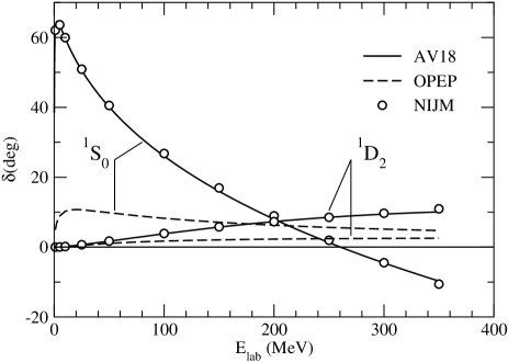
Figura 1.4: Comparison between the ¹S₀ and ¹D₂ phase shifts resulting from the Nijmegen analysis [35] (open circles) and the predictions of the Argonne $v_{18}$ (AV1 8) and one-pion-exchange (OPEP) potentials.

The calculations discussed in this Thesis are based on a widely employed potential model, obtained within the phenomenological approach outlined in this Section, generally referred to as Argonne $v_{18}$ potential [36]. It is written in the form

$$v(ij)=\sum_{n=1}^{18}v^{n}(r_{ij})O^{n}_{ij}\ .$$ (1.22)

As an example of the quality of the phase shifts obtained from the Argonne $v_{18}$ potential, in Fig. 1.4 we show the results for the ¹S₀ and ¹D₂ partial waves, compared with the predictions of the one-pion-exchange model (OPEP).

Figura 1.5: Radial dependence of the NN potential describing the interaction between two nucleons in the state of relative angular momentum $\ell=0$, and total spin and isospin $S=0$ and $T=1$.

We have used a simplified version of the above potential, obtained including the operators $O^{n\leq 8}_{ij}$, originally proposed in Ref.[37]. It reproduces the scalar part of the full interaction in all S and P waves, as well as in the ³D₁ wave and its coupling to the ³S₁.

The typical shape of the NN potential in the state of relative angular momentum $\ell=0$ and total spin and isospin $S=0$ and $T=1$ is shown in Fig. 1.5. The short-range repulsive core, to be ascribed to heavy-meson exchange or to more complicated mechanisms involving nucleon constituents, is followed by an intermediate-range attractive region, largely due to two-pion-exchange processes. Finally, at large interparticle distance the one-pion-exchange mechanism dominates.

1.1.2 Three-nucleon interactions

The NN potential determined from the properties of the two-nucleon system can be used to solve the many-body nonrelativistic Schrödinger equation for $A>2$. In the case $A=3$ the problem can be still solved exactly, but the resulting ground state energy, $E_{0}$, turns out to be slightly different from the experimental value. For example, for ³He one typically finds $E_{0}=7.6$ MeV, to be compared to $E_{exp}=8.48$ MeV. In order to exactly reproduce $E_{exp}$ one has to add to the nuclear hamiltonian a term containing three-nucleon interactions described by a potential $V_{ijk}$. The most important process leading to three-nucleon interactions is two-pion exchange associated with the excitation of a nucleon resonance in the intermediate state, depicted in Fig. 1.6.

Figura 1.6: Diagrammatic representation of the process providing the main contribution to the three-nucleon interaction. The thick solid line corresponds to an excited state of the nucleon.

The three-nucleon potential is usually written in the form

$$V_{ijk}=V_{ijk}^{2\pi}+V_{ijk}^{N}\ ,$$ (1.23)

where the first contribution takes into account the process of Fig. 1.6 while $V_{ijk}^{N}$ is purely phenomenological. The two parameters entering the definition of the three-body potential are adjusted in such a way as to reproduce the properties of ³H and ³He [38]. Note that the inclusion of $V_{ijk}$ leads to a very small change of the total potential energy, the ratio $\langle v_{ij}\rangle/\langle V_{ijk}\rangle$ being $\sim 2$ %.

For $A>3$ the Scrödinger equation is no longer exactly solvable. However, very accurate solutions can be obtained using stochastic techniques, such as variational Monte Carlo (VMC) Green function Monte Carlo (GFMC) [25].

The GFMC approach has been successfully employed to describe the ground state and the low lying excited states of nuclei having $A$ up to 10. The results of VMC and GFMC calculations carried out using realistic nuclear hamiltonian, summarized in Fig. 1.7, show that the nonrelativistic approach, based on a dynamics modeled to reproduce the properties of two- and three-nucleon systems, has a remarkable predictive power.

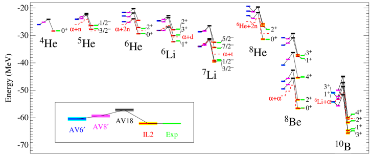
Figura 1.7: VMC and GFMC energies of nuclei with $A\leq 10$ compared to experiment (from Ref.[39]).

Capitolo 2 Nuclear matter theory

Understanding the properties of matter at densities comparable to the central density of atomic nuclei is made difficult by both the complexity of the interactions, discussed in the previous Chapter, and the approximations implied in any theoretical description of quantum mechanical many-particle systems.

The main problem associated with the use of the nuclear potential models described in Chapter 1 in a many-body calculation lies in the strong repulsive core of the NN force, which cannot be handled within standard perturbation theory.

In non-relativistic many-body theory (NMBT), a nuclear system is seen as a collection of point-like protons and neutrons whose dynamics are described by the hamiltonian

$$H=\sum_{i}t(i)+\sum_{j>i}v(ij)+\ldots\ ,$$ (2.1)

where $t(i)$ and $v(ij)$ denote the kinetic energy operator and the bare NN potential, respectively, while the ellipses refer to the presence of additional many-body interactions (see Chapter 1).

Carrying out perturbation theory in the basis provided by the eigenstates of the noninteracting system requires a renormalization of the NN potential. This is the foundation of the widely employed approach developed by Brückner, Bethe and Goldstone, in which $v(ij)$ is replaced by the well-behaved G-matrix, describing NN scattering in the nuclear medium (see, e.g. Ref.[40]). Alternatively, the many-body Schrödinger equation, with the hamiltonian of Eq.(2.1), can be solved using either the variational method or stochastic techniques. These approaches have been successfully applied to the study of both light nuclei [25] and uniform neutron and nuclear matter [28, 26, 27, 42].

Our work has been carried out using a scheme, formally similar to standard perturbation theory, in which nonperturbative effects due to the short-range repulsion are embodied in the basis functions. The details of this approach will be discussed in the following Sections.

It has to be emphasized that within NMBT the interaction is completely determined by the analysis of the exactly solvable two- and three-nucleon systems. As a consequence, the uncertainties associated with the dynamical model and the many-body calculations are decoupled, and the properties of nuclear systems ranging from deuteron to neutron stars can be obtained in a fully consistent fashion, without including any adjustable parameters.

2.1 Correlated basis function theory

The correlated states of nuclear matter are obtained from the Fermi gas (FG) states $|n_{FG}\rangle$ through the transformation [43, 44]

$$|n)=\frac{F|n_{{\rm FG}}\rangle}{\langle n_{{\rm FG}}|F^{\dagger}F|n_{{\rm FG}}\rangle^{1/2}}\ .$$ (2.2)

In the above equation, $|n_{{\rm FG}}\rangle$ is a determinant of single particle states describing $N$ noninteracting nucleons. The operator $F$, embodying the correlation structure induced by the NN interaction, is written in the form

$$F(1,\ldots,N)=\mathcal{S}\prod_{j>i=1}^{N}f_{ij}\ ,$$ (2.3)

where $\mathcal{S}$ is the symmetrization operator which takes care of the fact that, in general,

$$\left[f_{ij},f_{ik}\right]\neq 0\ .$$ (2.4)

The structure of the two-body correlation functions $f_{ij}$ must reflect the complexity of the NN potential. Hence, it is generally cast in the form (compare to Eq.(1.17))

$$f_{ij}=\sum_{n=1}^{6}f^{n}(r_{ij})O^{n}_{ij}\ ,$$ (2.5)

with the $O^{n}_{ij}$ defined by Eq.(1.16). Note that the operators included in the above definition provide a fairly accurate description of the correlation structure of the two-nucleon bound state. The shape of the radial functions $f^{n}(r_{ij})$ is determined through functional minimization of the expectation value of the nuclear hamiltonian in the correlated ground state

$$E^{V}_{0}=(0|H|0)\ .$$ (2.6)

The correlated states defined in Eq.(2.2) are not orthogonal to one another. However, they can be orthogonalized using an approach, based on standard techniques of many-body theory, that preserves diagonal matrix elements of the hamiltonian [45]. Denoting the orthogonalized states by $|n\rangle$, the procedure of Ref. [45] amounts to defining a transformation ${\widehat{T}}$ such that

$$|n)\rightarrow|n\rangle={\widehat{T}}|n)\ ,$$ (2.7)

with

$$(n|H|n)=\langle n|H|n\rangle\ .$$ (2.8)

Correlated basis function (CBF) perturbation theory is based on the decomposition of the nuclear hamiltonian

$$H=H_{0}+H_{I}\ ,$$ (2.9)

where $H_{0}$ and $H_{I}$ denote the diagonal and off-diagonal components of $H$, respectively, defined by the equations

$$\langle m|H_{0}|n\rangle = \delta_{mn}\langle m|H|n\rangle\ ,$$ (2.10)

$$\langle m|H_{I}|n\rangle = (1-\delta_{mn})\langle m|H|n\rangle\ .$$ (2.11)

The above definitions obviously imply that, if the correlated states have large overlaps with the eigenstates of $H$, the matrix elements of $H_{I}$ are small, and the perturbative expansions in powers of $H_{I}$ is rapidly convergent.

Let us consider, for example, the Green function describing the propagation of a nucleon in a hole state [46]

$$G({\bf k},\omega)=\langle\widetilde{0}|a^{\dagger}_{{\bf k}}\ \frac{1}{H-E_{0}-\omega-i\eta}\ a_{{\bf k}}|\widetilde{0}\rangle/\langle\widetilde{0}|\widetilde{0}\rangle\ .$$ (2.12)

In the above equation, $\eta=0^{+}$, $a^{\dagger}_{{\bf k}}$ and $a_{{\bf k}}$ are creation and annihilation operators and the exact ground state $|\widetilde{0}\rangle$, satisfying the Schrödinger equation $H|\widetilde{0}\rangle=E_{0}|\widetilde{0}\rangle$ can be obtained from the expansion [47, 48]

$$|\widetilde{0}\rangle=\sum_{n}(-)^{n}\left(\frac{H_{I}-\Delta E_{0}}{H_{0}-E_{0}^{V}}\right)^{n}|0\rangle\ ,$$ (2.13)

where $\Delta E_{0}=E_{0}-E^{V}_{0}$, with $E^{V}_{0}$ defined by Eq.(2.6).

In principle, using Eq.(2.13) and the similar expansion [47, 48]

$$\frac{1}{H-E_{0}-\omega-i\eta}=\frac{1}{H_{0}-E^{V}_{0}-\omega-i\eta}\ \sum_{n}(-)^{n}\left(\frac{H_{I}-\Delta E_{0}}{H_{0}-E^{V}_{0}-\omega-i\eta}\right)^{n}\ ,$$ (2.14)

the Green function can be consistently computed at any order in $H_{I}$. However, the calculation of the matrix elements of the hamiltonian appearing in Eqs.(2.12)-(2.14) involves prohibitive difficulties and requires the development of a suitable approximation scheme, to be discussed in the following Section.

2.2 Cluster expansion formalism

The correlation operator of Eq.(2.3) is defined such that, if any subset of the particles, say $i_{1},\ldots i_{p}$, is removed far from the remaining $i_{p+1},\ldots i_{N}$, it factorizes according to

$$F(1,\ldots,N)\rightarrow F_{p}(i_{1},\ldots i_{p})F_{N-p}(i_{p+1},\ldots i_{N})\ .$$ (2.15)

The above property is the basis of the cluster expansion formalism, that allows one to write the matrix element of a many-body operator between correlated states as a sum, whose terms correspond to contributions arising from isolated subsystems (clusters) involving an increasing number of particles.

Note that in this Section we will use non normalized correlated states, defined as (compare to Eq.(2.2))

$$|n\rangle=F|n_{FG}\rangle\ .$$ (2.16)

2.2.1 Ground state expectation value of the hamiltonian

Let us consider, as an example, the expectation value of the hamiltonian $H$ in the correlated state $|0\rangle$, defined in Eq.(2.16). We will closely follow the derivation of the corresponding cluster expansion given in Ref. [44] and neglect, for the sake of simplicity, the three body potential $V_{ijk}$. Under this assumption, we can write the hamiltonian as in Eq.(2.1).

The starting point is the definition of the generalized normalization integral

$$I(\beta)=\langle 0|{\rm exp}[\beta(H-T_{0})]|0\rangle\ ,$$ (2.17)

where

$$T_{0}=\sum_{|{\bf p}|<p_{F}}\frac{{\bf p}^{2}}{2m}\ ,$$ (2.18)

$p_{F}$ being the Fermi momentum, is the ground state energy of the noninteracting Fermi gas at density $\rho=2p_{F}^{3}/3\pi^{2}$. Using the definition of Eq.(2.17) we can rewrite the expectation value of the hamiltonian in the form

$$\langle H\rangle=\frac{\langle 0|H|0\rangle}{\langle 0|0\rangle}=T_{0}+\left.\frac{\partial}{\partial\beta}\ln I(\beta)\right|_{\beta=0}\ .$$ (2.19)

The cluster property of $F$ can be exploited to define a set of $N!/(N-p)!p!$ sub-normalization integrals, associated with each $p$-particle subsystem ($p=1,\ldots,N$)

$$I_{i}(\beta) = \langle i|{\rm exp}[\beta(t(1)-\epsilon^{0}_{i})]|i\rangle\ ,$$

$$I_{ij}(\beta) = \langle ij|F^{\dagger}_{2}(12){\rm exp}[\beta(t(1)+t(2)+v(12)-\epsilon^{0}_{i}-\epsilon^{0}_{j})]F_{2}(12)|ij\rangle_{a}\ ,$$

$$\vdots$$

$$I_{1\ldots N}(\beta) = I(\beta)\ ,$$ (2.20)

where the indices $i,j,\ldots$ label states belonging to the Fermi sea, the ket $|i_{1}\ldots i_{n}\rangle$ describes $n$ non interacting particles in the states $i_{1}\ldots i_{n}$, $\epsilon^{0}_{i}=|{\bf p}|_{i}^{2}/2m$ is the kinetic energy eigenvalue associated with the state $|i\rangle$ and the subscript $a$ refers to the fact that the corresponding state is antisymmetrized. For example, in the case of two particles

$$|ij\rangle_{a}=\frac{1}{\sqrt{2}}\ \left(|ij\rangle-|ji\rangle\right)\ .$$ (2.21)

To express $\ln I(\beta)$ in terms of the $\ln I_{i_{1}\ldots i_{p}}(\beta)$, we start noting that $I_{ij}$ is close to the product of $I_{i}$ and $I_{j}$. It would be exactly equal if we could neglect the interaction, described by the potential $v(12)$, and the correlations induced by both $F_{2}(12)$ and Pauli exclusion principle. This observation suggests that $I_{ij}$ can be written as

$$I_{ij}=I_{i}I_{j}Y_{ij}\ ,$$ (2.22)

with $Y_{ij}\sim 1$. Extending the same argument to the $I$’s with more than two indices, we obtain

$$I_{i} = Y_{i}$$

$$I_{ij} = Y_{i}Y_{j}Y_{ij}$$

$$\vdots$$

$$I_{1\ldots N} = I=\prod_{i}Y_{i}\ \prod_{j>i}Y_{ij}\ldots Y_{1\ldots N}\ ,$$ (2.23)

implying

$$\ln I(\beta)=\sum_{i}\ln Y_{i}+\sum_{j>i}\ln Y_{ij}+\ldots+\ln Y_{1\ldots N}\ .$$ (2.24)

It can be shown [44] that each term in the rhs of Eq.(2.24) goes like $N$ in the thermodynamic limit. In addition, the $p$-th term collects all contributions to the cluster development of $\ln I(\beta)$ involving, in a connected manner, exactly $p$ Fermi sea orbitals. Therefore, the $p$-th term can be referred to as the $p$-body cluster contribution to $\ln I(\beta)$.

The decomposition (2.23) allows one to rewrite the expectation value of the hamiltonian in the form

$$\langle H\rangle=T_{0}+(\Delta E)_{2}+(\Delta E)_{3}+\ldots+(\Delta E)_{N}$$ (2.25)

with

$$(\Delta E)_{p}=\sum_{i_{1}<i_{2}<\ldots<i_{p}}\left.\frac{\partial}{\partial\beta}\ln Y_{i_{1}i_{2}\ldots i_{p}}\right|_{\beta=0}\ .$$ (2.26)

Note that $(\Delta E)_{1}=0$, as the above definitions imply

$$I_{i}=Y_{i}=1\ ,$$ (2.27)

and

$$\frac{\partial I_{i}}{\partial\beta}=0\ .$$ (2.28)

To make the last step we have to use Eq.(2.23) and express $(\Delta E)_{p}$ in terms of the $I_{i_{1}\ldots i_{p}}$. Substitution of the resulting expressions

$$Y_{i} = I_{i}$$

$$Y_{ij} = I_{ij}(I_{i}I_{j})^{-1}\ ,$$ (2.29)

$$\vdots$$ (2.30)

into Eq.(2.26) with $p=2$ yields

$$(\Delta E)_{2}=\sum_{i<j}\left[\frac{1}{I_{ij}}\frac{\partial I_{ij}}{\partial\beta}-\left(\frac{\partial I_{i}}{\partial\beta}+\frac{\partial I_{j}}{\partial\beta}\right)\right]_{\beta=0}\ .$$ (2.31)

The “normalizations” $I_{ij}|_{\beta=0}$ appearing in the denominator differ from unity by terms $O(1/N)$ at most, that can be disregarded in the $N\rightarrow\infty$ limit. As a result, we obtain

$$(\Delta E)_{2}=\sum_{i<j}\ w_{ij}\ ,$$ (2.32)

where (see Eq.(2.20))

$$w_{ij}=\langle ij|\ \frac{1}{2}[F_{2}(12),\ [t(1)+t(2),\ F_{2}(12)]\ ]+F_{2}(12)v(12)F_{2}(12)\ |ij\rangle_{a}\ ,$$ (2.33)

Note that in the above equation we have assumed that the correlation operator be hermitian, i.e. that $F_{2}(12)=F^{\dagger}_{2}(12)=f_{12}$ (see Eq.(2.3)). The explicit expression of $(\Delta E)_{2}$, in the case of six component potential and correlation operator, is given in Appendix B.

Each term of the expansion (2.25) can be represented by a diagram featuring $p$ vertices, representing the nucleons in the cluster, connected by lines corresponding to dynamical and statistical correlations. The terms in the resulting diagrammatic expansion can be classified according to their topological structure, and selected classes of diagrams can be summed up to all orders solving a set of coupled integral equations, called Fermi hyper-netted chain (FHNC) equations [49, 50].

2.2.2 Transition matrix elements

The nuclear matter response to an external probe delivering energy $\omega$ and momentum ${\bf q}$ can be written in the form

$$S({\bf q},\omega)=\sum_{f}|\langle f|\mathcal{O}({\bf q})|0\rangle|^{2}\delta(\omega+E_{0}-E_{f})\ ,$$ (2.34)

where $\mathcal{O}$ is the operator inducing a transition from the ground state $|0\rangle$, carrying energy $E_{0}$, to a final state $|f\rangle$, carrying energy $E_{f}$. In the simple case of interaction with a scalar probe, resulting in a density fluctuation

$$\mathcal{O}({\bf q})=\rho({\bf q})=\sum_{{\bf k}}a^{\dagger}_{{\bf k}+{\bf q}}a_{{\bf k}}\ ,$$ (2.35)

$a^{\dagger}_{{\bf k}}$ and $a_{{\bf k}}$ being nucleon creation and annihilation operators, respectively.

In order to obtain the response within the CBF approach, the cluster expansion formalism discussed in the previous section must be extended to the case of transition matrix elements.

Consider a (non normalized) correlated one particle-one hole final state

$$|f\rangle=|{\bf p}{\bf h}\rangle=Fa^{\dagger}_{{\bf p}}a_{{\bf h}}|0_{FG}\rangle\ .$$ (2.36)

To obtain the response we need to calculate the matrix elements

$$\frac{\langle 0|\rho_{{\bf q}}^{\dagger}|{\bf p}{\bf h}\rangle}{\langle 0|0\rangle^{1/2}\langle{\bf p}{\bf h}|{\bf p}{\bf h}\rangle^{1/2}}$$ (2.37)

The cluster expansion of the above quantity can be carried out using a formalism somewhat different from the one described in the previous Section, originally developed in Ref. [51]. The starting point is again the generalized normalization integral, that in this case is written in the form

$$I_{0,ph}(\beta,\alpha)=\sqrt{N!}\int\prod_{i=1}^{N}dx_{i}\ \Phi_{0}^{\dagger}(1,\ldots,N)F^{\dagger}\ {\rm e}^{\beta\rho_{{\bf q}}^{\dagger}}F\ {\rm e}^{\alpha W_{ph}}\ \phi_{m_{1}}(1)\ldots\phi_{m_{N}}(N)\ ,$$ (2.38)

In the above equation $x_{1},\ldots,\ x_{N}$ denote the nucleon degrees of freedom, and $\Phi_{0}^{\dagger}(1,\ldots,N)=\langle x_{1}\ldots x_{N}|0_{FG}\rangle$ is the FG ground state wave function, i.e. the antisymmetrized product of the single particle orbitals $\phi_{m_{1}}(1)\ldots\phi_{m_{N}}N(N)$. Note that the calculation of matrix elements involving states describing Fermi systems, only requires the antisymmetrization of either the initial or the final state. The coordinate space expressions of the operators $\rho_{{\bf q}}$ and $W_{ph}$ are

$$\rho_{{\bf q}}=\sum_{i=1}^{N}\ {\rm e}^{i{\bf q}\cdot{\bf r}_{i}}\ =\sum_{i=1}^{N}\ \rho_{{\bf q}}(i)\ ,$$ (2.39)

$$W_{ph}=\sum_{i=1}^{N}\ \frac{\phi_{p}(i)}{\phi_{m_{i}}(i)}\delta_{hm_{i}}=\sum_{i=1}^{N}\ W_{ph}(i)\ .$$ (2.40)

Acting on the product $\phi_{m_{1}}\ldots\phi_{m_{N}}$, $W_{ph}$ replaces the hole state orbital $\phi_{m_{i}}$ with the particle state orbital $\phi_{p}$. In terms of generalized normalization integrals we can write

$$\langle{\bf p}{\bf h}|\rho_{{\bf q}}^{\dagger}|0\rangle=\int\prod_{i=1}^{N}dx_{i}\ \Phi_{0}^{\dagger}F^{\dagger}\rho_{{\bf q}}^{\dagger}\ F\Phi_{0}=\left.\frac{\partial}{\partial\beta}\frac{\partial I_{0,ph}(\beta,\alpha)}{\partial\alpha}\right|_{\alpha=\beta=0}\ ,$$ (2.41)

$$\langle{\bf p}{\bf h}|{\bf p}{\bf h}\rangle=\int\prod_{i=1}^{N}dx_{i}\Phi_{ph}^{\dagger}F^{\dagger}\ F\Phi_{ph}=I_{ph,ph}(0,0)$$ (2.42)

where $I^{ph,ph}(0,\alpha)$ is obtained from Eq.(2.38) replacing the FG ground state with the one particle-one hole state $\Phi_{ph}$, and

$$\langle 0|0\rangle=\int\prod_{i=1}^{N}dx_{i}\Phi_{0}^{\dagger}F^{\dagger}\ F\Phi_{0}=I_{0,0}(0,0)\ .$$ (2.43)

To carry out the cluster expansion we need to define subnormalization integrals, involving an increasing number of orbitals

$$I_{i} = \int dx_{1}\phi_{m_{i}}(1){\rm e}^{\beta\rho_{{\bf q}}^{\dagger}(1)}{\rm e}^{\alpha W_{ph}(1)}\phi_{m_{i}}(1)=X_{i}$$

$$I_{ij} = \sqrt{2}\int dx_{1}dx_{2}\ \varphi_{m_{i}m_{j}}^{\dagger}(1,2)F_{2}^{\dagger}(12){\rm e}^{\beta[\rho_{{\bf q}}^{\dagger}(1)+\rho_{{\bf q}}^{\dagger}(2)]}F_{2}(12)$$

$$\times {\rm e}^{\alpha[W_{ph}(1)+W_{ph}(2)]}\phi_{m_{i}}(1)\phi_{m_{j}}(2)=X_{i}X_{j}+X_{ij}$$

$$\vdots$$

$$I_{1\ldots N} = I^{0,ph}(\beta,\alpha)=\sum\ X_{i_{1}\ldots a}\ldots X_{j_{1}\ldots b}\ ,$$ (2.44)

where $\varphi_{m_{i}m_{j}}(1,2)=[\phi_{m_{i}}(1)\phi_{m_{j}}(2)-\phi_{m_{i}}(2)\phi_{m_{j}}(1)]/\sqrt{2})$, and the sum in the last line is extended to all partitions such that $a\leavevmode\nobreak\ +\leavevmode\nobreak\ \ldots\leavevmode\nobreak\ +\leavevmode\nobreak\ b\leavevmode\nobreak\ =\leavevmode\nobreak\ N$. Note that in this case the (small) deviation between $I_{ij}$ and the product $I_{i}I_{j}$ is characterized through their difference, rather than the ratio (compare to Eq.(2.23)).

The thermodynamic limit (i.e. the limit $A,V\rightarrow\infty$, with $A/V={\rm const}$) of $I_{0,ph}(\beta,\alpha)$ can be best identified rewriting it in the form originally obtained in Ref. [51]:

$$I_{0,ph}(\beta,\alpha)=\prod_{i=1}^{N}X_{i}(\beta,\alpha){\rm e}^{G_{0,ph}(\beta,\alpha)}\ ,$$ (2.45)

with

$$G_{0,ph}=\sum_{j>i}\xi_{ij}+O(N^{-1})\ ,$$ (2.46)

where

$$\xi_{ij}=\frac{X_{ij}}{X_{i}X_{j}}\ .$$ (2.47)

Defining

$$\mathcal{P}_{0,ph}(\beta)=\left[\frac{\partial\ {\rm e}^{G_{0,ph}(\beta,\alpha)}}{\partial\alpha}\right]_{\alpha=0}\ {\rm e}^{-[G_{ph,ph}(0,0)+G_{0,0}(0,0)]/2}$$ (2.48)

we finally obtain [51]

$$\frac{\langle 0|\rho_{{\bf q}}^{\dagger}|{\bf p}{\bf h}\rangle}{\langle 0|0\rangle^{1/2}\langle{\bf p}{\bf h}|{\bf p}{\bf h}\rangle^{1/2}}=\langle({\bf p}{\bf h})_{FG}|\rho_{{\bf q}}^{\dagger}|0_{FG}\rangle\ \mathcal{P}_{0,ph}(0)+\left.\frac{\partial}{\partial\beta}\mathcal{P}_{0,ph}(\beta)\right|_{\beta=0}\ .$$ (2.49)

From the above equations it follows that, at two-body cluster level [51],

$$\frac{\langle 0|\rho_{{\bf q}}^{\dagger}|{\bf p}{\bf h}\rangle}{\langle 0|0\rangle^{1/2}\langle{\bf p}{\bf h}|{\bf p}{\bf h}\rangle^{1/2}}=\sum_{i}\left.\frac{\partial}{\partial\beta}\frac{\partial X_{i}}{\partial\alpha}\right|_{\beta=\alpha=0}+\sum_{j>i}\left.\frac{\partial}{\partial\beta}\frac{\partial X_{ij}}{\partial\alpha}\right|_{\beta=\alpha=0}\ .$$ (2.50)

Note that the derivation of Eq.(2.50) has been carried out consistently with that of Eq.(2.31), i.e. neglecting all contributions $O(N^{-1})$ to the normalization of the correlated two-nucleon states.

2.3 Effective interaction

At lowest order of CBF, the effective interaction $V_{{\rm eff}}$ is defined by the equation

$$\langle H\rangle=\langle 0_{FG}|T_{0}+V_{{\rm eff}}|0_{FG}\rangle\ .$$ (2.51)

As the above equation suggests, the approach based on the effective interaction allows one to obtain any nuclear matter observables using perturbation theory in the FG basis. However, as discussed in the previous Section, the calculation of the hamiltonian expectation value in the correlated ground state, needed to extract $V_{{\rm eff}}$ from Eq.(2.51), involves severe difficulties.

In this Thesis we follow the procedure developed in Refs. [52, 31], whose authors derived the expectation value of the effective interaction by carrying out a cluster expansion of the rhs of Eq.(2.51), and keeping only the two-body cluster contribution. The resulting expression, that can be obtained from Eqs.(2.26)-(2.33) through a simple rearrangement of the kinetic energy contributions, reads

$$\langle 0_{FG}|V_{{\rm eff}}|0_{FG}\rangle=\sum_{i<j}\langle ij|v_{{\rm eff}}(12)|ij\rangle_{a}$$

$$\ \ \ \ =\sum_{i<j}\langle ij|f_{12}\left[-\frac{1}{m}(\nabla^{2}f_{12})-\frac{2}{m}(\bm{\nabla}f_{22})\cdot\bm{\nabla}+v(12)f_{12}\right]|ij\rangle_{a}\ ,$$ (2.52)

where the laplacian and the gradient operate on the relative coordinate. Note that $v_{{\rm eff}}$ defined by the above equation exhibits a momentum dependence due to the operator $(\bm{\nabla}f_{ij})\cdot\bm{\nabla}$, yielding contributions to nuclear matter energy through the exchange terms . However, our numerical calculations show that these contributions are small, compared to the ones associated with the momentum independent terms. As a consequence, the results presented in this Thesis have been obtained using only the static part of the effective interaction (2.52), i.e. setting

$$v_{{\rm eff}}(ij)=f_{ij}\left(-\frac{1}{m}\nabla^{2}+v(ij)\right)f_{ij}=\sum_{n}v_{{\rm eff}}^{n}(r_{ij})O^{n}_{ij}\ ,$$ (2.53)

The properties of the operators $O^{n}$ with $n=1,\ldots,\ 6$, leading to the above result, are given in Appendix A.

The definition of $v_{{\rm eff}}$ given by Eqs.(2.52) and (2.53) obviously neglects the effect of three-nucleon interactions, whose inclusion in the hamiltonian is known to be needed in order to explain the binding energies of the few-nucleon systems, as well as the saturation properties of nuclear matter. To circumvent this problem, we have used the approach originally proposed by Lagaris and Pandharipande [53], in which the main effect of the three-body force is simulated through a density dependent modification of the two-nucleon potential at intermediate range, where two-pion exchange is believed to be the dominant interaction mechanism. Neglecting, for simplicity, the charge-symmetry breaking components of the interaction, the resulting potential can be written in the form

$$\widetilde{v}(ij)=\sum_{n=1,14}\left[v^{n}_{\pi}(r_{ij})+v^{n}_{I}(r_{ij}){\rm e}^{-\gamma_{1}\rho}+v^{n}_{S}(r_{ij})\right]O^{n}_{ij}\ ,$$ (2.54)

where $v^{n}_{\pi}$, $v^{n}_{I}$ and $v^{n}_{S}$ denote the long- (one-pion-exchange), intermediate- and short-range part of the potential, respectively. The above modification results in a repulsive contribution to the binding energy of nuclear matter. The authors of Ref.[53] also include the small additional attractive contribution

$$\Delta E_{TNA}=\gamma_{2}\rho^{2}(3-2\beta^{2}){\rm e}^{-\gamma_{3}\rho}\ ,$$ (2.55)

with $\beta=(\rho_{p}-\rho_{n})/(\rho_{p}+\rho_{n})$, where $\rho_{p}$ and $\rho_{n}$ denote the proton and neutron density, respectively. The values of the parameters $\gamma_{1}$, $\gamma_{2}$ and $\gamma_{3}$ appearing in Eqs.(2.54) and (2.55) have been determined in such a way as to reproduce the binding energy and equilibrium density of nuclear matter [53].

Besides the bare two- and three body-potentials, the effective interaction is determined by the correlation operators $f_{ij}$ defined by Eq.(2.5). The shapes of the radial functions $f^{n}(r_{ij})$ are obtained from the functional minimization of the energy at the two-body cluster level, yielding a set of coupled differential equations to be solved with the boundary conditions

$$f^{n}(r_{ij}\geq d)=\left\{\begin{array}[]{ll}1\ ,&n=1\\ 0\ ,&n=2,3,4\\ \end{array}\right.\ ,$$ (2.56)

$$f^{n}(r_{ij}\geq d_{t})=0\ ,\ n=5,6$$ (2.57)

and

$$\left.\frac{df^{n}}{dr_{ij}}\right|_{r_{ij}=d} = 0\ ,\ n=1,2,3,4$$

$$\left.\frac{df^{n}}{dr_{ij}}\right|_{r_{ij}=d_{t}} = 0\ ,\ n=5,6\ ,$$ (2.58)

$d$ and $d_{t}>d$ being variational parameters. The above conditions simply express the requirements that i) for relative distances larger than the interaction range the two-nucleon wave function reduces to the one describing non interacting particles and ii) tensor interactions have longer range.

For any given value of nuclear matter density, we have solved the Euler-Lagrange equations resulting from the minimization of the binding energy at two-body cluster level, whose derivation and explicit form is given in Appendix C, using the values of $d$ and $d_{t}$ reported in Ref.[54].

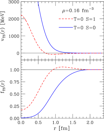
Figura 2.1: Interaction potentials (upper panel) and correlation functions (lower panel) acting in the spin-isospin channels $S=0$ and $T=0$ (solid lines) and $S=0$ and $T=1$ (dashed lines). The potential is the Argonne $v^{\prime}_{8}$ and the correlation functions correspond to nuclear matter at equilibrium density.

As an example, the results corresponding to nuclear matter at equilibrium density are illustrated in Fig.2.1, showing the central component of the correlation functions acting between a pair of nucleon carrying total spin and isospin $S$ and $T$, respectively. The relations between the $f_{TS}$ of Fig.2.1 and the $f^{n}$ of Eq.(2.5) are given in Appendix A. The shapes of the $f_{TS}$ clearly reflect the nature of the interaction. In the $T=0$ $S=0$ channel, in which the potential exhibits a strong repulsive core, the correlation function is very small at $r\mathrel{\hbox to0.0pt{\lower 4.0pt\hbox{\hskip 1.0pt$\sim$}\hss}\raise 1.0pt\hbox{$<$}}0.5$ fm. On the other hand, in the $T=0$ $S=1$ channel, the spin-isospin state corresponding to the deuteron, the repulsive core is much weaker and the potential becomes attractive at $r\mathrel{\hbox to0.0pt{\lower 4.0pt\hbox{\hskip 1.0pt$\sim$}\hss}\raise 1.0pt\hbox{$>$}}0.7$ fm. As a consequence, the correlation function does not approach zero as $r\rightarrow 0$ and exceeds unity at intermediate range.

In Fig.2.2 the components of the effective interaction at equilibrium density are compared to the corresponding components of the truncated $v_{8}^{\prime}$ potential. It clearly appears that screening effects due to NN correlations lead to a significant quenching of the interaction.

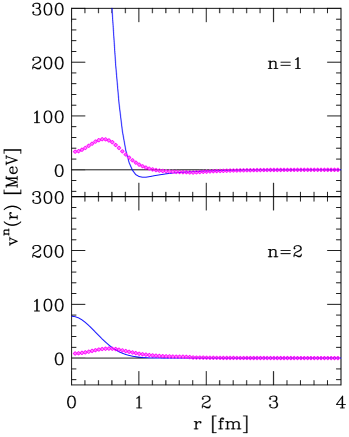
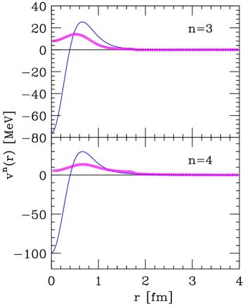
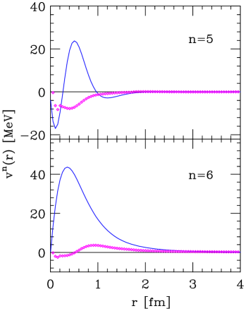
Figura 2.2: Comparison between the components of the bare Argonne $v^{\prime}_{8}$ potential (dashed lines) and the effective potential defined by Eq.(2.53) (solid lines), calculated at nuclear matter equilibrium density.

Figure 2.3 shows a comparison between the central ($n=1$, left panel) and spin-isospin ($n=4$, right panel) components of the effective interaction of Eq.(2.53), calculated at different densities using the Argonne $v^{\prime}_{8}$ potential. The density dependence is associated with the correlation functions, which depend on $\rho$ through the correlation ranges, $d$ and $d_{t}$, and the Fermi distributions. The jumps in the radial behavior of the effective interactions, clearly visible in Figs. 2.2 and 2.3 are due to the discontinuity in the second derivative of the correlation functions.

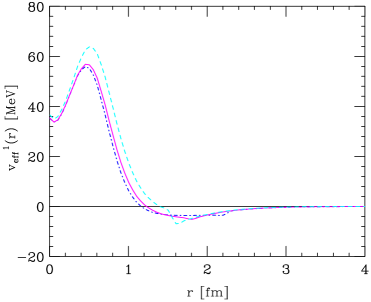
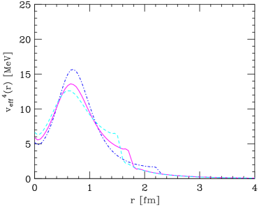
Figura 2.3: Density dependence of the central ($n=1$, left panel) and spin-isospin ($n=4$, right panel) components of the effective interaction of Eq.(2.53), calculated using the Argonne $v^{\prime}_{8}$ potential. The dot-dash, dashed and solid lines correspond to $\rho=$ 0.04, 0.16 and 0.32 fm^-3, respectively.

2.3.1 Energy per particle of neutron and nuclear matter

The effective interaction described in the previous Section was tested by computing the energy per particle of symmetric nuclear matter and pure neutron matter in first order perturbation theory using the FG basis.

Let us consider nuclear matter at density

$$\rho=\sum_{\lambda=1}^{4}\ \rho_{\lambda}\ ,$$ (2.59)

where $\lambda=1,2,3,4$ labels spin-up protons, spin-down protons, spin-up neutrons and spin-down neutrons, respectively, the corresponding densities being $\rho_{\lambda}=x_{\lambda}\rho$, with $\sum_{\lambda}x_{\lambda}=1$. For example, for symmetric nuclear matter $x_{1}=x_{2}=x_{3}=x_{4}=1/4$, while for pure neutron matter $x_{1}=x_{2}=0$ and $x_{3}=x_{4}=1/2$. Within our approach, the energy of such a system can be obtained from

$$\frac{E}{N}=\frac{3}{5}\ \sum_{\lambda}\frac{p_{F,\lambda}^{2}}{2m}+\frac{\rho}{2}\sum_{\lambda\mu}\sum_{n}\ x_{\lambda}x_{\mu}\int d^{3}r\ v^{n}_{{\rm eff}}\left[A^{n}_{\lambda\mu}-B^{n}_{\lambda\mu}\ell(p_{F,\lambda}r)\ell(p_{F,\mu}r)\right]\ .$$ (2.60)

In the above equation, $p_{F,\lambda}=(6\pi^{2}\rho_{\lambda})^{1/3}$ and the Slater function $\ell$ is defined as

$$\ell(p_{F,\lambda}r)=\sum_{\bf k}\ {\rm e}^{i{\bf k}\cdot{\bf r}}\ \theta(p_{F,\lambda}-|{\bf k}|)\ .$$ (2.61)

The explicit expression of the matrices

$$A^{n}_{\lambda\mu}=\langle\lambda\mu|O^{n}|\lambda\mu\rangle\ \ ,\ \ B^{n}_{\lambda\mu}=\langle\lambda\mu|O^{n}|\mu\lambda\rangle\ ,$$ (2.62)

where $|\lambda\mu\rangle$ denotes the two-nucleon spin-isospin state, is given in Appendix A.

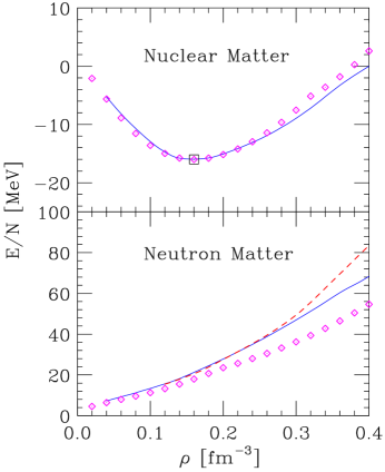
Figura 2.4: Energy per particle of symmetric nuclear matter (upper panel) and pure neutron matter (lower panel). The solid lines represent the results obtained using Eq.(2.60), whereas the diamonds correspond to the results of Akmal, Pandharipande and Ravenhall [41]. The dashed line of the lower panel represents the results of the AFDMC approach or Ref. [27]. The square in the upper panel shows the empirical saturation point of symmetric nuclear matter.

In Fig. 2.4 our results are compared to those of Refs. [41] and [27]. The calculations of Ref. [41] (diamonds, results given in the sixth column of Table VI) have been carried out using a variational approach based on the FHNC-SOC formalism, with a hamiltonian including the Argonne $v_{18}$ NN potential and the Urbana IX three-body potential [38]. The results of Ref. [27] (dashed line of the lower panel) have been obtained using the $v_{8}^{\prime}$ model and the same three-body potential, within the framework of the Auxiliary field diffusion Monte Carlo (AFDMC) technique. It appears that the effective interaction approach provides a fairly reasonable description of the EOS over a broad density range.

The comparison between the results of our calculation, based on the two-body cluster approximation, and those obtained taking into account higher order many-body effects deserves a comment. In view of the fact that the contribution of clusters involving more than two nucleons is known to be sizable, our approach has to be regarded as an effective theory, designed to provide lowest order results in agreement with the available “data”. Effective theories are widely employed in many areas of Physics, including nuclear matter theory. For example, the Walecka model [55] is designed to reproduce the nuclear matter empirical saturation properties in the mean field approximation, i.e. at tree level, although the corresponding loop corrections are known to be large.

It is worth noting that the empirical equilibrium properties of symmetric nuclear matter are accounted for without including the somewhat ad hoc density dependent correction of Ref. [41]. The authors of Ref. [32] argued that this may be ascribed to the different description of the three-body force. It should also be emphasized that, using $v_{{\rm eff}}$ of Eq.(2.53) and the three-nucleon interaction (TNI) model of Ref. [53], one effectively includes the contribution of clusters involving more than two nucleons.

In addition to the correct binding energy per nucleon and equilibrium density ($E/N=15.96$ MeV at $\rho=0.16$ fm^-3), our calculation also yields a quite reasonable value of the compressibility module, $K=$ 230 MeV.

It has to be kept in mind that our approach does not involve adjustable parameters. The correlation ranges $d$ and $d_{t}$ have been taken from Ref. [54], while the parameters entering the definition of the TNI have been determined by the authors of Ref. [53] through a fit of nuclear matter equilibrium properties.

2.3.2 Single particle spectrum and effective mass

Using the effective interaction, the effective mass can be obtained from the single-particle energies $e_{\lambda}({\bf p})$, that can be easily computed in Hartree-Fock approximation [46]. The resulting expression is (compare to Eq.(2.60)):

$$e_{\lambda}(p)=\frac{p^{2}}{2m}+\rho\ \sum_{\mu}\sum_{n}x_{\mu}\int d^{3}rv^{n}_{\rm eff}(r)\left[A^{n}_{\lambda\mu}-B^{n}_{\lambda\mu}j_{0}(pr)\ell(p_{F,\mu}r)\right]\ ,$$ (2.63)

where $p=|{\bf p}|$ and $j_{0}$ is the spherical Bessel function: $j_{0}(x)=\sin(x)/x$. Figure 2.5 shows $e(p)=\sum_{\lambda}x_{\lambda}e_{\lambda}(p)$ for symmetric nuclear matter at equilibrium density. For comparison the corresponding results from Ref. [57] are also displayed. They have been obtained using the FHNC-SOC approach and the Urbana $v_{14}$ two-nucleon potential, modified according to the TNI model of Lagaris and Pandharipande [53].

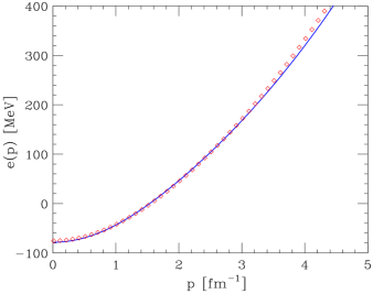
Figura 2.5: Solid Line: momentum dependence of the single particle energies obtained from the CBF effective interaction in the Hartree-Fock approximation (see Eq.(2.63)). The diamonds show the results of Ref.[57].

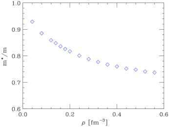
Figura 2.6: Density dependence of the ratio $m^{\star}(p_{F})/m$ of PNM, obtained from Eqs.(2.63) and (2.64) using the effective interaction described in the text.

The nucleon effective mass, $m^{\star}$, is related to the single-particle energy through

$$\frac{1}{m^{\star}}=\frac{1}{p}\ \frac{de}{dp}\ .$$ (2.64)

The density dependence of the ratio $m^{\star}(p_{F})/m$ of PNM, obtained from the $v_{\rm eff}$ discussed in this Chapter, is shown in Fig. 2.6. It is worth mentioning that for SNM at equilibrium, we find $m^{\star}(p_{F})/m=0.65$, in close agreement with the lowest order CBF result of Ref. [56]. The results of CBF calculations at second order show a $\sim$20% enhancement of the effective mass at the Fermi surface, due to medium polarization effects [56]. We do not find this enhancement, as these effects are not taken into account in the Hartree-Fock approximation.

2.3.3 Spin susceptibility of neutron matter

The results of numerical calculations show that the energy per particle of nuclear matter can be accurately approximated using the expression

$$\frac{1}{N}\ E(\alpha,\beta,\gamma)=E_{0}+E_{\sigma}\alpha^{2}+E_{\tau}\beta^{2}+E_{\sigma\tau}\gamma^{2}\ ,\$$ (2.65)

with

$$\alpha = (x_{3}-x_{4})+(x_{1}-x_{2})$$

$$\beta = (x_{3}+x_{4})-(x_{1}+x_{2})$$ (2.66)

$$\gamma = (x_{3}-x_{4})-(x_{1}-x_{2})\ .$$

In symmetric nuclear matter $x_{\lambda}=1/4$ for all $\lambda$ (see the definition in Section 2.3.2), yielding $E/N=E_{{\rm SNM}}=E_{0}$, while in pure neutron matter, corresponding to $x_{1}=x_{2}=0$ and $x_{3}=x_{4}=1/2$, $E/N=E_{{\rm PNM}}=E_{0}+E_{\tau}$, implying that $E_{\tau}$ can be identified with the symmetry energy.

Let us consider fully spin-polarized neutron matter. The two degenerate states corresponding to $x_{3}=1$ and $x_{4}=0$ ($\alpha=1$, spin-up) and $x_{3}=0$ and $x_{4}=1$ ($\alpha=-1$, spin-down) have energy,

$$E^{\uparrow}=E^{\downarrow}=E_{{\rm PNM}}+\widetilde{E}_{\sigma}\ ,$$ (2.67)

with $\widetilde{E}_{\sigma}=E_{\sigma}+E_{\sigma\tau}$. For arbitrary polarization $\alpha$, the energy can be obtained from the expansion

$$E(\alpha)=E(0)+\left.\frac{\partial E}{\partial\alpha}\right|_{\alpha=0}\alpha+\frac{1}{2}\left.\frac{\partial^{2}E}{\partial\alpha^{2}}\right|_{\alpha=0}\alpha^{2}+\ldots\ .$$ (2.68)

As $E$ must be an even function of $\alpha$ (see Eq.(2.67)), the linear term in the above series must be vanishing and, neglecting terms of order $\alpha^{3}$, we can write

$$\Delta E=E(\alpha)-E(0)=\frac{1}{2}\left.\frac{\partial^{2}E}{\partial\alpha^{2}}\right|_{\alpha=0}\alpha^{2}\ .$$ (2.69)

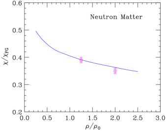
Figura 2.7: Ratio between the spin susceptibility obtained from Eqs.(2.75) and (2.60) and the FG model result. The points with error bars show the AFDMC results of Ref.[58].

In the presence of a uniform magnetic field ${\bf B}$ the energy of the system becomes

$$E_{B}(\alpha)=E(\alpha)-\alpha\mu B,$$ (2.70)

where $B$ denotes the magnitude of the external field, whose direction is chosen as spin quantization axis, and $\mu$ is the neutron magnetic moment.

Assuming that equilibrium is achieved at $\alpha=\alpha_{0}$, i.e. that

$$\left.\frac{\partial E}{\partial\alpha}\right|_{\alpha=\alpha_{0}}-\mu B=0\ ,$$ (2.71)

we obtain

$$\alpha_{0}=\mu B\left(\frac{\partial^{2}E}{\partial\alpha^{2}}\right)^{-1}_{\alpha=0}\ .$$ (2.72)

From the definitions of the total magnetization

$$M=\mu(\rho_{3}-\rho_{4})=\mu\alpha_{0}\rho=\mu^{2}\left(\frac{\partial^{2}E}{\partial\alpha^{2}}\right)^{-1}_{\alpha=0}B\rho\ ,$$ (2.73)

and the spin susceptibility $\chi$

$$M=\chi B\ ,$$ (2.74)

we finally obtain

$$\chi=\mu^{2}\left(\frac{\partial^{2}E}{\partial\alpha^{2}}\right)^{-1}_{\alpha=0}\rho=\mu^{2}\frac{1}{2(E^{\uparrow}-E_{{\rm PNM}})}\ \rho\ .$$ (2.75)

The above equation shows that, within our approach, the spin susceptibility of neutron matter can be easily calculated from Eq.(2.60)

Figure 2.7 shows the density dependence of the ratio between the susceptibility of neutron matter obtained from the effective interaction and that corresponding to the FG model. For comparison, the results of Ref.[58], obtained within the AFDMC approach using the Argonne $v^{\prime}_{8}$ NN potential and the Urbana IX three-body force, are also displayed. It appears that the inclusion of interactions leads to a substantial decrease of the susceptibility over the whole density range, and that the agreement between the two theoretical calculations is remarkably good.

Capitolo 3 Nuclear matter response

In this Chapter, we will discuss the response of nuclear matter to an external probe, defined in Eq.(2.34) of Chapter 2. Extensive experimental studies of the nuclear response have been carried out mostly through inclusive electron scattering experiments (for a recent review see, e.g., [9]). The wealth of available data, corresponding to a variety of targets, ranging from the few nucleon systems, having $A\leq 4$, to nuclei as heavy as Gold ($A=197$) and Lead ($A=208$), can be reliably extrapolated to the $A\rightarrow\infty$ limit to obtain quantitative empirical information on the nuclear matter response [59].

Electron scattering experiments have exposed the deficiencies of the independent particle model of nuclear dynamics. On the other hand, many body approaches explicitly including dynamical correlation effects provide a quantitative account of the measured cross sections in a broad kinematical domain [9].

As a pedagogical example, we will first consider the response to a scalar probe. The generalization to the case of electromagnetic and charged current weak interactions will be discussed in Chapters 4 and 5.

3.1 Many-body theory of the nuclear response

Within NMBT, the nuclear response to a scalar probe delivering momentum q and energy $\omega$, defined in Eq.(2.34), can be written in terms of the the imaginary part of the polarization propagator $\Pi({\bf q},\omega)$ according to [46, 48]

$$S({\bf q},\omega)=\frac{1}{\pi}\ {\rm Im}\ \Pi({\bf q},\omega)=\frac{1}{\pi}\ {\rm Im}\ \langle 0|\rho^{\dagger}_{{\bf q}}\ \frac{1}{H-E_{0}-\omega-i\eta}\ \rho_{{\bf q}}|0\rangle\ ,$$ (3.1)

where $\eta=0^{+}$ denotes an infinitesimal positive quantity and the operator $\rho_{{\bf q}}$, describing the density fluctuation induced by the probe, is given in Eq(2.35).

The above definition is best suited to establish the relation between $S({\bf q},\omega)$ and the nucleon Green function, leading to the popular expression of the response in terms of spectral functions [48, 47].

Equation (3.1) clearly shows that the interaction with the probe leads to a transition of the struck nucleon from a hole state of momentum ${\bf k}$, with $|{\bf k}|<p_{F}$, to a particle state of momentum ${\bf k}+{\bf q}$, with $|{\bf k}+{\bf q}|>p_{F}$. Hence, the calculation of $S({\bf q},\omega)$ amounts to describing the propagation of a particle-hole pair through the nuclear medium.

The Green function is the quantum mechanical amplitude associated with the propagation of a particle from $x\equiv(t,{\bf x})$ to $x^{\prime}\equiv(t^{\prime},{\bf x}^{\prime})$ [46]. In uniform matter, due to translation invariance, it only depends on the difference $x-x^{\prime}$, and after Fourier transformation to the conjugate variable $k\leavevmode\nobreak\ \equiv\leavevmode\nobreak\ (\leavevmode\nobreak\ {\bf k}\leavevmode\nobreak\ ,\leavevmode\nobreak\ E\leavevmode\nobreak\ )$ can be written in the form

$$G({\bf k},E) = \langle 0|a^{\dagger}_{{\bf k}}\ \frac{1}{H-E_{0}-E-i\eta}\ a_{{\bf k}}|0\rangle-\langle 0|a_{{\bf k}}\ \frac{1}{H-E_{0}+E-i\eta}\ a^{\dagger}_{{\bf k}}|0\rangle$$ (3.2)

$$= G_{h}({\bf k},E)+G_{p}({\bf k},E)\ ,$$

where $G_{h}$ and $G_{p}$ correspond to propagation of nucleons in hole and particle states, respectively.

The connection between Green function and spectral functions is established through the Lehman representation[46]

$$G({\bf k},E)=\int dE^{\prime}\left[\frac{P_{h}({\bf k},E^{\prime})}{E^{\prime}-E-i\eta}-\frac{P_{p}({\bf k},E^{\prime})}{E-E^{\prime}-i\eta}\right]\ ,$$ (3.3)

implying

$$P_{h}({\bf k},E)=\sum_{n}|\langle n_{(N-1)}(-{\bf k})|a_{{\bf k}}|0_{N}\rangle|^{2}\delta(E-E^{(-)}_{n}+E_{0})=\frac{1}{\pi}\ {\rm Im}\ G_{h}({\bf k},E)\ ,$$ (3.4)

$$P_{p}({\bf k},E)=\sum_{n}|\langle n_{(N+1)}({\bf k})|a^{\dagger}_{{\bf k}}|0_{N}\rangle|^{2}\delta(E+E^{(+)}_{n}-E_{0})=\frac{1}{\pi}{\rm Im}\ G_{p}({\bf p},E)\ ,$$ (3.5)

where $|\langle n_{(N\pm 1)}(\pm{\bf k})\rangle$ denotes an eigenstate of the $(A\pm 1)$-nucleon system, carrying momentum $\pm{\bf k}$ and energy $E^{(\pm)}_{n}$.

Within the FG model the matrix elements of the creation and annihilation operators reduce to step functions, and the Green function takes a very simple form. For example, for hole states we find

$$G_{FG,h}({\bf k},E)=\frac{\theta(p_{F}-|{\bf k}|)}{E+\epsilon^{0}_{k}-i\eta}\ ,$$ (3.6)

with $\epsilon^{0}_{k}=|{\bf k}^{2}|/2m$, implying

$$P_{FG,h}({\bf k},E)=\theta(p_{F}-|{\bf k}|)\delta(E+\epsilon^{0}_{k})\ .$$ (3.7)

Strong interactions modify the energy of a nucleon carrying momentum ${\bf k}$ according to $\epsilon^{0}_{k}\longrightarrow\epsilon^{0}_{k}+\Sigma({\bf k},E)$, where $\Sigma({\bf k},E)$ is the complex nucleon self-energy, describing the effect of nuclear dynamics. As a consequence, the Green function for hole states becomes

$$G_{h}({\bf k},E)=\frac{1}{E+\epsilon^{0}_{k}+\Sigma({\bf k},E)}\ .$$ (3.8)

A very convenient decomposition of $G_{h}({\bf k},E)$ can be obtained inserting a complete set of $(A-1)$-nucleon states (see Eqs.(3.2)-(3.4)) and isolating the contributions of one-hole bound states, whose weight is given by[60]

$$Z_{k}=|\langle-{\bf k}|a_{{\bf k}}|0\rangle|^{2}=\theta(p_{F}-|{\bf k}|)\Phi_{k}\ .$$ (3.9)

Note that in the FG model these are the only non-vanishing terms, and $\Phi_{k}\equiv 1$, while in the presence of interactions $\Phi_{k}<1$. The resulting contribution to the Green function exhibits a pole at $-\epsilon_{k}$, the quasi-particle energy $\epsilon_{k}$ being defined by the equation

$$\epsilon_{k}=\epsilon^{0}_{k}+{\rm Re}\ \Sigma({\bf k},\epsilon_{k})\ .$$ (3.10)

The full Green function can be rewritten

$$G_{h}({\bf k},E)=\frac{Z_{k}}{E+\epsilon_{k}+iZ_{k}\ {\rm Im}\ \Sigma({\bf k},e_{k})}+G^{B}_{h}({\bf k},E)\ ,$$ (3.11)

where $G^{B}_{h}$ is a smooth contribution, associated with $(A-1)$-nucleon states having at least one nucleon excited to the continuum (two hole-one particle, three hole-two particles …) due to virtual scattering processes induced by nucleon-nucleon (NN) interactions. The corresponding spectral function is

$$P_{h}({\bf k},E)=\frac{1}{\pi}\ \frac{Z_{k}^{2}\ {\rm Im}\ \Sigma({\bf k},\epsilon_{k})}{[E+\epsilon^{0}_{k}+{\rm Re}\ \Sigma({\bf k},\epsilon_{k})]^{2}+[Z_{k}{\rm Im}\ \Sigma({\bf k},\epsilon_{k})]^{2}}+P^{B}_{h}({\bf k},E)\ .$$ (3.12)

The first term in the right hand side of the above equation yields the spectrum of a system of independent quasi-particles, carrying momenta $|{\bf k}|<p_{F}$, moving in a complex mean field whose real and imaginary parts determine the quasi-particle effective mass and lifetime, respectively. The presence of the second term is a consequence of nucleon-nucleon correlations, not taken into account in the mean field picture. Being the only one surviving at $|{\bf k}|>p_{F}$, in the FG model this correlation term vanishes.

Figura 3.1: Energy dependence of the hole spectral function of nuclear matter.[47] The solid, dashed and dot-dash lines correspond to $|{\bf k}|=$ 1, 0.5 and 1.5 fm^-1, respectively. The FG spectral function at $|{\bf k}|=$ 1 and 0.5 fm^-1 is shown for comparison. The quasi-particle strengths of Eq.(3.9), are also reported.

Figure 3.1 illustrates the energy dependence of the hole spectral function of nuclear matter, calculated in Ref.[47] using CBF perturbation theory and a realistic nuclear hamiltonian, including the Urbana $v_{14}$ potential and the TNI discussed in the previous Chapter. Comparison with the FG model clearly shows that the effects of nuclear dynamics and NN correlations are large, resulting in a shift of the quasi-particle peaks, whose finite width becomes large for deeply-bound states with $|{\bf k}|\ll p_{F}$. In addition, NN correlations are responsible for the appearance of strength at $|{\bf k}|>p_{F}$. The energy integral

$$n(k)=\int dE\ P_{h}({\bf k},E)$$ (3.13)

yields the occupation probability of the state of momentum ${\bf k}$. The results of Fig. 3.1 clearly show that in presence of correlations $n(|{\bf k}|>p_{F})\neq 0$.

3.2 Nuclear response and spectral functions

In general, the calculation of the response requires the knowledge of $P_{h}$ and $P_{p}$, as well as of the particle-hole effective interaction.[48, 61] The spectral functions are mostly affected by short range NN correlations (see Fig. 3.1), while the inclusion of the effective interaction, e.g. within the framework of the Tamm-Dancoff approximation (TD) or the Random Phase Approximation (RPA), [61] is needed to account for collective excitations induced by long range correlations, involving more than two nucleons.

At large momentum transfer, as the space resolution of the probe becomes small compared to the average NN separation distance, $S({\bf q},\omega)$ is no longer significantly affected by long range correlations. The authors of Ref. [62] found that for $|{\bf q}|\mathrel{\hbox to0.0pt{\lower 4.0pt\hbox{\hskip 1.0pt$\sim$}\hss}\raise 1.0pt\hbox{$>$}}$ 500 MeV RPA corrections are negligibly small, if computed using finite size interactions.

In this kinematical regime the zero-th order approximation in the effective interaction, according to which hole and particle propagate independent of one another, is expected to be applicable. The corresponding response can be written in the simple form

$$S({\bf q},\omega)=\int d^{3}kdE\ P_{h}({\bf k},E)P_{p}({\bf k}+{\bf q},\omega-E)\ .$$ (3.14)

The widely employed plane wave impulse approximation (IA) [9] can be readily obtained from the above definition replacing $P_{p}$ with the FG result, which amounts to disregarding final state interactions (FSI) between the struck nucleon and the spectator particles. The resulting expression reads

$$S_{IA}({\bf q},\omega)=\int d^{3}kdE\ P_{h}({\bf k},E)\theta(|{\bf k}+{\bf q}|-p_{F})\delta(\omega-E-\epsilon^{0}_{|{\bf k}+{\bf q}|})\ .$$ (3.15)

Figure 3.2, showing the $\omega$ dependence of the nuclear matter structure function at $|{\bf q}|=5$ fm^-1, illustrates the role of correlations in the target ground state. The solid and dashed lines have been obtained from Eq.(3.15) using the spectral function of Ref.[47] and that resulting from the FG model (shifted in such a way as to account for nuclear matter binding energy), respectively. It clearly appears that the inclusion of correlations produces a significant shift of the strength towards larger values of energy transfer.

Figura 3.2: Nuclear matter $S_{IA}({\bf q},\omega)$ (see Eq.(3.15)), as a function of $\omega$ at $|{\bf q}|=5$ fm^-1. The solid and dashed lines correspond to the spectral function of Ref.[47] and to the FG model (shifted in such a way as to account for nuclear matter binding energy), respectively (taken from Ref.[63]).

At moderate momentum transfer, both the full response and the particle and hole spectral functions can be obtained using non relativistic many-body theory. The results of Ref.[47] suggest that the zero-th order approximations of Eqs.(3.14) and (3.15) are fairly accurate at $|{\bf q}|\leavevmode\nobreak\ \mathrel{\hbox to0.0pt{\lower 4.0pt\hbox{\hskip 1.0pt$\sim$}\hss}\raise 1.0pt\hbox{$>$}}\leavevmode\nobreak\ 500$ MeV. However, in this kinematical regime the motion of the struck nucleon in the final state can no longer be described using the non relativistic formalism. While at IA level this problem can be easily circumvented replacing the non relativistic kinetic energy with its relativistic counterpart, including the effects of FSI in the response of Eq.(3.14) involves further approximations, needed to obtain the particle spectral function at large $|{\bf q}|$.

3.3 Particle spectral function at large momentum

A systematic scheme to include corrections to Eq.(3.15) and take into account FSI, originally proposed in Ref.[64], is discussed in Ref.[65]. The main effects of FSI on the response are i) a shift in energy, due to the mean field of the spectator nucleons and ii) a redistributions of the strength, due to the coupling of the one particle-one hole final state to $n$ particle-$n$ hole final states.

In the simplest implementation of the approach of Refs.[64, 65], the response is obtained from the IA result according to

$$S({\bf q},\omega)=\int d\omega^{\prime}\ S_{IA}({\bf q},\omega^{\prime})f_{{\bf q}}(\omega-\omega^{\prime})\ ,$$ (3.16)

the folding function $f_{{\bf q}}$ being related to the particle spectral function through

$$P_{p}({\bf k}+{\bf q},\omega-E)=\theta(k_{F}-|{\bf k}+{\bf q}|)\ f_{|{\bf k}+{\bf q}|}(\omega-E-e^{0}_{|{\bf k}+{\bf q}|})$$ (3.17)

with $\epsilon^{0}_{|{\bf k}+{\bf q}|}=\sqrt{|{\bf k}+{\bf q}|^{2}+m^{2}}$. In the absence of FSI, $f_{{\bf q}}$ shrinks to a $\delta$-function and the IA result of Eq.(3.15) is recovered.

Obviously, at large ${\bf q}$ the calculation of $P_{p}({\bf k}+{\bf q},\omega-E)$ cannot be carried out using a nuclear potential model. However, it can be obtained form the measured NN scattering amplitude within the eikonal approximation. The resulting folding function is the Fourier transform of the Green function describing the propagation of the struck particle, travelling in the direction of the $z$-axis with constant velocity $v$:

$$f_{|{\bf q}|}(\omega)=\int\frac{dt}{2\pi}\ {\rm e}^{i\omega t}{\rm e}^{i\int_{0}^{t}dt^{\prime}{\widetilde{V}}_{|{\bf q}|}(vt^{\prime})}\ .$$ (3.18)

where ${\bf k}+{\bf q}\approx{\bf q}$ and

$${\widetilde{V}}_{|{\bf q}|}(z)=\langle 0|\frac{1}{A}\sum_{j>i}\Gamma_{|{\bf q}|}({\bf r}_{ij}+{\bf z})|0\rangle\ .$$ (3.19)

In the above equation, $\Gamma_{|{\bf q}|}$ is the Fourier transform of the NN scattering amplitude at incident momentum $|{\bf q}|$ and momentum transfer $|{\bf t}|$, $A_{|{\bf q}|}(k)$, parameterized according to

$$A_{|{\bf q}|}(p)=\frac{|{\bf q}|}{4\pi}\sigma(i+\alpha){\rm e}^{-\beta p^{2}}\ .$$ (3.20)

In principle, the total cross section $\sigma$, the slope $\beta$ and the ratio between the real and the imaginary part, $\alpha$, can be extracted from NN scattering data. However, the modifications of the scattering amplitude due to the presence of the nuclear medium are known to be sizable, and must be taken into account. The calculation of these corrections within the framework of NMBT is discussed in Ref.[66].

In Eq.(3.19), the expectation value is evaluated in the correlated ground state. It turns out that NN correlation, whose effect on $P_{h}$ is illustrated in Fig. 3.1, also affect the particle spectral function and, as a consequence, the folding function of Eq. (3.17). Neglecting all correlations

$${\widetilde{V}}_{|{\bf q}|}(z)\rightarrow{\widetilde{V}}^{0}_{|{\bf q}|}=\frac{1}{2}v\rho\sigma(i+\alpha)\ ,$$ (3.21)

and the quasi-particle approximation

$$P_{p}({\bf q},\omega-E)=\frac{1}{\pi}\frac{{\rm Im}\ {\widetilde{V}}^{0}_{|{\bf q}|}}{\left[\omega-E-e^{0}_{|{\bf q}|}-{\rm Re}\ {\widetilde{V}}^{0}_{|{\bf q}|}\right]^{2}+\left[{\rm Im}\ {\widetilde{V}}^{0}_{|{\bf q}|}\right]^{2}}$$ (3.22)

is recovered.

Correlations induce strong density fluctuations, preventing two nucleon from coming close to one another. The joint probability of finding two particles at positions ${\bf r_{1}}$ and ${\bf r_{2}}$ can be written

$$\rho({\bf r_{1}},{\bf r_{2}})=\langle 0|\sum_{j>i}\delta({\bf r}_{i}-{\bf r}_{1})\delta({\bf r}_{j}-{\bf r}_{2})|0\rangle=\rho^{2}g(|{\bf r_{1}}-{\bf r_{2}}|)\ .$$ (3.23)

The above equation defines the radial distribution function $g(r)$, which describes correlation effects. Figure 3.3 shows the typical shape of the radial distribution function resulting from the CBF calculation of Ref. [67].

Figura 3.3: Radial distribution function of nuclear matter at equilibrium density, obtained from CBF perturbation theory using a realistic hamiltonian [67].

The effect of correlation on FSI can be easily understood keeping in mind that the response is only sensitive to rescattering taking place within a distance $\sim 1/|{\bf q}|$ of the primary interaction vertex As the probability of finding a spectator within the range of the repulsive core of the NN force ($\mathrel{\hbox to0.0pt{\lower 4.0pt\hbox{\hskip 1.0pt$\sim$}\hss}\raise 1.0pt\hbox{$<$}}1$ fm) is small, the probability that the struck particle rescatter against one of the spectators within a length $\sim 1/|{\bf q}|$ is also very small at large $|{\bf q}|$. Hence, inclusion of correlations leads to a significant suppression of FSI.

Figura 3.4: Nuclear matter $S({\bf q},\omega)$, defined in Eq.(3.16), as a function of $\omega$ at $|{\bf q}|=5$ fm^-1. The solid and dashed lines have been obtained from the spectral function of Ref.[47], with and without inclusion of FSI, respectively. The dot-dash line corresponds to the FG model (shifted in such a way as to account for nuclear matter binding energy), respectively (taken from Ref. [63]).

Fig. 3.4 shows the $\omega$ dependence of the nuclear matter response of Eq.(3.16) at $|{\bf q}|=5$ fm^-1. The solid and dashed lines have been obtained using the spectral function of Ref.[47], with and without inclusion of FSI according to the formalism of Ref.[64], respectively. For reference, the results of the FG model are also shown by the dot-dash line. The two effects of FSI, energy shift and redistribution of the strength from the region of the peak to the tails, clearly show up in the comparison between solid and dashed lines.

Capitolo 4 Impulse Approximation regime

As pointed out in the previous Chapter, the nuclear response has been extensively investigated carrying out inclusive electron scattering experiments.

The first attempts to provide a quantitative estimate the of the measured electron-nucleus cross section were based on oversimplified models of nuclear dynamics. At the end of the seventies, Moniz suggested that the target may be described as a degenerate gas of protons and neutrons at given constant density $\rho$ [68], the effect of the interactions being crudely taken into account by an average binding energy $\overline{\epsilon}$. Despite its simplicity, the FG model of Ref. [68] was able to give a fairly accurate account of the electron-nucleus cross section in the region of the quasi-elastic peak, corresponding to $x_{B}=Q^{2}/2m\omega\ \sim$ 1, where $x_{B}$ is the Bjorken variable, $Q^{2}=|{\bf q}|^{2}-\omega^{2}$, and $\bf{q}$, $\omega$ and $m$ denote the momentum and energy transfer and the nucleon mass, respectively.

In the past twenty years, with the availability of new data, extending in the region of high $|{\bf q}|$ and low $\omega$, corresponding to $x_{B}\gg 1$, the limits of the FG model, and more generally of all independent particle models, became apparent. Away from the quasi elastic peak correlation effects, not included in the mean field picture, become more and more important and the FG model is not longer able to describe the measured cross section.

The experimental investigation of the neutrino-nucleus cross section involves additional difficulties due to the low counting rates and the lack of neutrino beams of fully specified properties. However, a quantitative understanding of the weak nuclear response is needed in a variety of different fields, ranging from nuclear astrophysics to the analysis of neutrino oscillation experiments.

Electron scattering data provide a stringent test for validation of theoretical models of the nuclear response, in view of their application to the case of weakly interacting probes. For example, the success of the FG model in explaining electron scattering in the quasi elastic region at $|{\bf q}|\mathrel{\hbox to0.0pt{\lower 4.0pt\hbox{\hskip 1.0pt$\sim$}\hss}\raise 1.0pt\hbox{$<$}}$ 500 MeV prompted its extension to neutrino scattering [69].

In this Chapter we will review the application of the formalism on NMBT to the calculation of the electromagnetic and charged current weak cross sections in the region of large momentum transfer, where the IA is expected to be safely applicable.

4.1 Electron-nucleus cross section

The differential cross section of the process

$$e+A\rightarrow e^{\prime}+X\ ,$$ (4.1)

in which an electron carrying initial four-momentum $k\equiv(E_{e},{\bf k})$ scatters off a nuclear target to a state of four-momentum $k^{\prime}\equiv(E_{e}^{\prime},{\bf k}^{\prime})$, the target final state being undetected, can be written in Born approximation as (see, e.g., Ref. [70])

$$\frac{d^{2}\sigma}{d\Omega_{e^{\prime}}dE_{e}^{\prime}}=\frac{\alpha^{2}}{Q^{4}}\frac{E_{e}^{\prime}}{E_{e}}\ L^{\mu\nu}W_{\mu\nu}^{A}\ ,$$ (4.2)

where $\alpha$ is the fine structure constant. The leptonic tensor, that can be written, neglecting the lepton mass, as

$$L^{\mu\nu}=2\left[k_{\mu}k_{\nu}^{\prime}+k_{\nu}k_{\mu}^{\prime}-g_{\mu\nu}(kk^{\prime})\right]\ ,$$ (4.3)

is completely determined by electron kinematics, whereas the nuclear tensor $W_{\mu\nu}^{A}$ contains all the information on target structure. Its definition involves the initial and final hadronic states $|0\rangle$ and $|X\rangle$, carrying four-momenta $p_{0}$ and $p_{X}$, respectively, as well as the nuclear electromagnetic current operator $J^{\mu}$:

$$W_{\mu\nu}^{A}=\sum_{X}\langle 0|J^{\mu}|X\rangle\langle X|J^{\nu}|0\rangle\delta^{(4)}(p_{0}+q-p_{X})\ ,$$ (4.4)

where the sum includes all hadronic final states. Comparison with Eq.(2.34) shows that the above tensor is the generalization of the nuclear response to the case of vector interaction.

Calculations of $W_{\mu\nu}^{A}$ at moderate momentum transfers $({\bf|q|}<0.5\,{\rm GeV})$ can be carried out within nuclear many-body theory (NMBT), using non-relativistic wave functions to describe the initial and final states and expanding the current operator in powers of ${\bf|q|}/m$, $m$ being the nucleon mass (see, e.g., Ref. [71, 72, 73]). On the other hand, at higher values of ${\bf|q|}$, corresponding to beam energies larger than $\sim 1$  GeV, the description of the final states $|X\rangle$ in terms of non-relativistic nucleons is no longer accurate. Calculations of $W_{\mu\nu}^{A}$ in this regime require a set of simplifying assumptions, allowing one to take into account the relativistic motion of final state particles carrying momenta $\sim{\bf q}$ as well as the occurrence of inelastic processes, leading to the appearance of hadrons other than protons and neutrons.

4.2 The impulse approximation

As stated in Chapter 3, the main assumptions underlying the impulse approximation (IA) scheme are that i) as the spatial resolution of a probe delivering momentum ${\bf q}$ is $\sim 1/|{\bf q}|$, at large enough $|{\bf q}|$ the target nucleus is seen by the probe as a collection of individual nucleons and ii) the particles produced at the interaction vertex and the recoiling (${\rm A}-1$)-nucleon system evolve independently of one another, which amounts to neglecting both statistical correlations due to Pauli blocking and dynamical Final State Interactions (FSI), i.e. rescattering processes driven by strong interactions.

In the IA regime the scattering process off a nuclear target reduces to the incoherent sum of elementary processes involving only one nucleon, as schematically illustrated in Fig. 4.1.

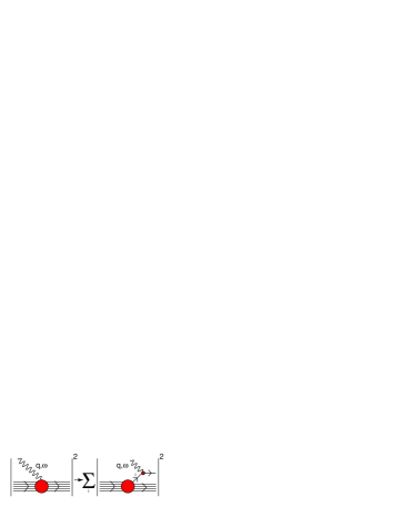
Figura 4.1: Schematic representation of the IA scheme, in which the nuclear cross section is replaced by the incoherent sum of cross sections describing scattering off individual bound nucleons, the recoiling $({\rm A}-1)$-nucleon system acting as a spectator.

Within this picture, the nuclear current can be written as a sum of one-body currents

$$J^{\mu}\rightarrow\sum_{i}j_{i}^{\mu}\ ,$$ (4.5)

while the final state reduces to the direct product of the hadronic state produced at the electromagnetic vertex, carrying momentum ${\bf p}_{x}$ and the $(A-1)$-nucleon residual system, carrying momentum ${\bf p}_{\cal R}={\bf q}-{\bf p}_{x}$ (for simplicity, we omit spin indices)

$$|X\rangle\rightarrow|x,{\bf p}_{x}\rangle\otimes|{\cal R},{\bf p_{\cal R}}\rangle\ .$$ (4.6)

Using Eq. (4.6) we can rewrite the sum in Eq. (4.4) replacing

$$\sum_{X}|X\rangle\langle X|\rightarrow\sum_{x}\int d^{3}p_{x}|x,{\bf p}_{x}\rangle\langle{\bf p}_{x},x|\ \sum_{{\cal R}}d^{3}p_{{\cal R}}|{\cal R},{\bf p}_{{\cal R}}\rangle\langle{\bf p}_{{\cal R}},{\cal R}|\ .$$

Substitution of Eqs. (4.5)-(4.2) into Eq. (4.4) and insertion of a complete set of free nucleon states, satisfying

$$\int d^{3}p\ |{\rm N},{\bf p}\rangle\langle{\bf p},{\rm N}|=I\ ,$$ (4.7)

results in the factorization of the current matrix element

$$\langle 0|J^{\mu}|X\rangle=\left(\frac{m}{\sqrt{{\bf p}_{{\cal R}}^{2}+m^{2}}}\right)^{1/2}\langle 0|{\cal R},{\bf p}_{{\cal R}};{\rm N},-{\bf p}_{{\cal R}}\rangle\sum_{i}\langle-{\bf p}_{\cal R},N|j^{\mu}_{i}|x,{\bf p}_{x}\rangle\ ,$$ (4.8)

leading to

$$W_{\mu\nu}^{A} = \sum_{x,{\cal R}}\int d^{3}p_{{\cal R}}\ d^{3}p_{x}|\langle 0|{\cal R},{\bf p}_{{\cal R}};{\rm N},-{\bf p}_{{\cal R}}\rangle|^{2}\ \frac{m}{E_{{\bf p}_{\cal R}}}$$

$$\times \sum_{i}\ \langle-{\bf p}_{{\cal R}},{\rm N}|j^{\mu}_{i}|x,{\bf p}_{x}\rangle\langle{\bf p}_{x},x|j^{\nu}_{i}|{\rm N},-{\bf p}_{{\cal R}}\rangle$$

$$\times \delta^{(3)}({\bf q}-{\bf p}_{{\cal R}}-{\bf p}_{x})\delta(\omega+E_{0}-E_{\cal R}-E_{x}),$$

where $E_{{\bf p}_{\cal R}}=\sqrt{|{\bf p}_{{\cal R}}|^{2}+m^{2}}$. Finally, using the identity

$$\delta(\omega+E_{0}-E_{\cal R}-E_{x})=\int dE\delta(E-m+E_{0}-E_{\cal R})\ \delta(\omega-E+m-E_{x})\ ,$$ (4.10)

and the definition of the target spectral function given in the previous Chapter,

$$P({\bf p},E)=\sum_{\cal R}|\langle 0|{\cal R},-{\bf p};{\rm N},{\bf p}\rangle|^{2}\ \delta(E-m+E_{0}-E_{\cal R})\ ,$$ (4.11)

we can rewrite Eq.(4.4) in the form

$$W_{\mu\nu}^{A}({\bf q},\nu)=\sum_{i}\int d^{3}p\ dE\ w_{i}^{\mu\nu}({\widetilde{q}})\left(\frac{m}{E_{{\bf p}}}\right)P({\bf p},E)\ ,$$ (4.12)

with $E_{{\bf p}}=\sqrt{|{\bf p}^{2}|+m^{2}}$ and

$$w_{i}^{\mu\nu}=\sum_{x}\langle{\bf p},{\rm N}|j^{\mu}_{i}|x,{\bf p}+{\bf q}\rangle\langle{\bf p}+{\bf q},x|j^{\nu}_{i}|{\rm N},{\bf p}\rangle\ \delta({\widetilde{\omega}}+\sqrt{{\bf p}^{2}+m^{2}}-E_{x})\ .$$

Note that the factor $(m/\sqrt{|{\bf p}_{{\cal R}}|^{2}+m^{2}})^{1/2}$ in Eq.(4.8) takes into account the implicit covariant normalization of $\langle-{\bf p}_{\cal R},N|$ in the matrix element of $j_{i}^{\mu}$.

The quantity defined in the above equation is the tensor describing electromagnetic interactions of the $i$-th nucleon in free space. Hence, Eq. (4.2) shows that in the IA scheme the effect of nuclear binding of the struck nucleon is accounted for by the replacement

$$q\equiv(\omega,{\bf q})\rightarrow{\widetilde{q}}\equiv({\widetilde{\omega}},{\bf q})\ ,$$ (4.13)

with (see Eqs. (4.2) and (4.11))

$${\widetilde{\omega}} = E_{x}-\sqrt{{\bf p}^{2}+m^{2}}$$ (4.14)

$$= \omega+E_{0}-E_{\cal R}-\sqrt{{\bf p}^{2}+m^{2}}$$

$$= \omega-E+m-\sqrt{{\bf p}^{2}+m^{2}}\ ,$$

in the argument of $w_{i}^{\mu\nu}$. This procedure essentially amounts to assuming that: i) a fraction $\delta\omega$ of the energy transfer goes into excitation energy of the spectator system and ii) the elementary scattering process can be described as if it took place in free space with energy transfer ${\widetilde{\omega}}=\omega-\delta\omega$. This interpretation emerges most naturally in the $|{\bf p}|\ll m$ limit, in which Eq. (4.14) yields $\delta\omega=E$.

Collecting together all the above results we can finally rewrite the doubly differential nuclear cross section in the form

$$\frac{d\sigma_{IA}}{d\Omega_{e^{\prime}}dE_{e^{\prime}}}=\int\ d^{3}p\ dE\ P({\bf p},E)\ \left[Z\frac{d\sigma_{ep}}{d\Omega_{e^{\prime}}dE_{e^{\prime}}}\right.$$

$$\ \ \ \ \ \ \ \ \ \ \ \ \ \ \ \ \ \ \ \ +\left.(A-Z)\frac{d\sigma_{en}}{d\Omega_{e^{\prime}}dE_{e^{\prime}}}\right]\delta(\omega-E+m-E_{x}),$$ (4.15)

where $d\sigma_{eN}/d\Omega_{e^{\prime}}dE_{e^{\prime}}$ ($N\equiv n,p$ denotes a proton or a neutron) is the cross section describing the elementary scattering process

$$e(k)\ +\ N(p)\rightarrow e^{\prime}(k^{\prime})+x(p+{\widetilde{q}})\ ,$$ (4.16)

given by

$$\frac{d\sigma_{eN}}{d\Omega_{e^{\prime}}dE_{e^{\prime}}}=\frac{\alpha^{2}}{Q^{4}}\frac{E_{e}^{\prime}}{E_{e}}\ \frac{m}{E_{\bf p}}L^{\mu\nu}w^{\mu\nu}_{N}\ ,$$ (4.17)

stripped of both the flux factor and the energy conserving $\delta$-function.

4.3 The nuclear spectral function

Non-relativistic NMBT provides a fully consistent computational framework that has been employed to obtain the spectral functions of the few-nucleon systems, having A$=3$ [74, 75, 76] and 4 [77, 78, 79], as well as of nuclear matter, i.e. in the limit A $\rightarrow\infty$ with Z=A/2 [47, 80]. Calculations based on G-matrix perturbation theory have also been carried out for oxygen [81, 82].

The spectral functions of different nuclei, ranging from Carbon to Gold, have been modeled using the Local Density Approximation (LDA) [83], in which the experimental information obtained from nucleon knock-out measurements is combined with the results of theoretical calculations of the nuclear matter $P({\bf p},E)$ at different densities [83].

Nucleon removal from shell model states has been extensively studied by coincidence $(e,e^{\prime}p)$ experiments (see, e.g., Ref. [22]). The corresponding measured spectral function is usually parameterized in the factorized form

$$P_{MF}({\bf p},E)=\sum_{n}Z_{n}\ |\phi_{n}({\bf p})|^{2}F_{n}(E-E_{n})\ ,$$ (4.18)

where $\phi_{n}({\bf p})$ is the momentum-space wave function of the single particle shell mode state $n$ (e.g. Woods-Saxon wave functions), whose energy width is described by the function $F_{n}(E-E_{n})$ (e.g. a lorentzian). The normalization of the $n$-th state is given by the so called spectroscopic factor $Z_{n}<1$, and the sum in Eq. (4.18) is extended to all occupied states. Typically, $P_{MF}({\bf p},E)$ vanishes at $E$ larger than $\sim 30$ MeV and $|{\bf p}|$ larger than $\sim 250$ MeV. Note that in absence of NN correlations the full spectral function could be written as in Eq. (4.18), with $F_{n}(E-E_{n})\equiv\delta(E-E_{n})$ and $Z_{n}\equiv 1$.

Strong dynamical NN correlations give rise to virtual scattering processes leading to the excitation of the participating nucleons to states of energy larger than the Fermi energy, thus depleting the shell model states within the Fermi sea. As a consequence, the spectral function associated with nucleons belonging to correlated pairs extends to the region of $|{\bf p}|\gg p_{F}$ and $E\gg e_{F}$, where $e_{F}$ denotes the Fermi energy, typically $\mathrel{\hbox to0.0pt{\lower 4.0pt\hbox{\hskip 1.0pt$\sim$}\hss}\raise 1.0pt\hbox{$<$}}30$ MeV.

The correlation contribution to $P({\bf p},E)$ of uniform nuclear matter has been calculated by Benhar et al for a wide range of density values [83]. Within the LDA scheme, the results of Ref. [83] can be used to obtain the corresponding quantity for a finite nucleus of mass number $A$ from

$$P_{corr}({\bf p},E)=\int d^{3}r\ \rho_{A}({\bf r})P^{NM}_{corr}({\bf p},E;\rho=\rho_{A}({\bf r}))\ ,$$ (4.19)

where $\rho_{A}({\bf r})$ is the nuclear density distribution and $P^{NM}_{corr}({\bf p},E;\rho)$ is the correlation component of the spectral function of uniform nuclear matter at density $\rho$.

Finally, the full LDA nuclear spectral function can be written

$$P_{LDA}({\bf p},E)=P_{MF}({\bf p},E)+P_{corr}({\bf p},E)\ ,$$ (4.20)

the spectroscopic factors $Z_{n}$ of Eq. (4.18) being constrained by the normalization requirement

$$\int d^{3}p\ dE\ P_{LDA}({\bf p},E)=1\ .$$ (4.21)

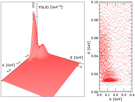
Figura 4.2: Three-dimensional plot (left panel) and scatter plot (right panel) of the oxygen spectral function obtained using the LDA approximation described in the text.

The LDA spectral function of ${}^{16}O$ obtained combining the nuclear matter results of Ref. [83] and the Saclay $(e,e^{\prime}p)$ data [84] is shown in Fig. 4.2. The shell model contribution $P_{MF}({\bf p},E)$ accounts for $\sim$ 80 % of its normalization, whereas the remaining $\sim$ 20 % of the strength, accounted for by $P_{corr}({\bf p},E)$, is located at high momentum ($|{\bf p}|\gg p_{F}$) and large removal energy ($E\gg e_{F}$). It has to be emphasized that large $E$ and large ${\bf p}$ are strongly correlated. For example, $\sim$ 50 % of the strength at $|{\bf p}|$ = 320 MeV is located at $E>$ 80 MeV.

The LDA scheme rests on the premise that short range nuclear dynamics is unaffected by surface and shell effects. The validity of this assumption is confirmed by theoretical calculations of the nucleon momentum distribution, defined as

$$n({\bf p})=\int dE\ P({\bf p},E)=\langle 0|a^{\dagger}_{\bf p}a_{\bf p}|0\rangle\ ,$$ (4.22)

where $a^{\dagger}_{\bf p}$ and $a_{\bf p}$ denote the creation and annihilation operators of a nucleon of momentum ${\bf p}$. The results clearly show that for A$\geq 4$ the quantity $n({\bf p})/A$ becomes nearly independent of $A$ in the region of large $|{\bf p}|$ ($\mathrel{\hbox to0.0pt{\lower 4.0pt\hbox{\hskip 1.0pt$\sim$}\hss}\raise 1.0pt\hbox{$>$}}300$ MeV), where NN correlations dominate (see, e.g., Ref. [85]).

In Fig. 4.3 the nucleon momentum distribution of ¹⁶O, obtained from Eq. (4.22) using the LDA spectral function of Fig. 4.2, is compared to the one resulting from a Monte Carlo calculation [86], carried out using the definition of Eq. (4.22) and a highly realistic many-body wave function [88]. For reference, the FG model momentum distribution corresponding to Fermi momentum $p_{F}$ = 221 MeV, currently used in the analysis of neutrino oscillation experiments (see, e.g. Ref.[87]), is also shown by the dashed line. It clearly appears that the $n({\bf p})$ obtained from the spectral function is close to that of Ref.[86], while the FG distribution exhibits a completely different behavior.

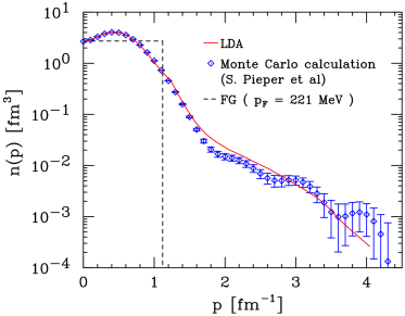
Figura 4.3: Momentum distribution of nucleons in the oxygen ground state. Solid line: LDA approximation. Dashed line: FG model with Fermi momentum $p_{F}=221$ MeV. Diamonds: Monte Carlo calculation carried out by S.C. Pieper [86] using the wave function of Ref. [88].

A direct measurement of the correlation component of the spectral function of ${}^{12}C$, obtained measuring the $(e,e^{\prime}p)$ cross section at missing momentum and energy up to $\sim$ 800 MeV and $\sim\leavevmode\nobreak\ 200$ MeV, respectively, has been recently carried out at Jefferson Lab by the E97-006 Collaboration [89]. The data resulting from the preliminary analysis appear to be consistent with the theoretical predictions based on LDA.

4.4 Comparison to electron scattering data

We have employed the formalism described in the previous Sections to compute the inclusive electron scattering cross section off oxygen at $0.2\mathrel{\hbox to0.0pt{\lower 4.0pt\hbox{\hskip 1.0pt$\sim$}\hss}\raise 1.0pt\hbox{$<$}}Q^{2}\mathrel{\hbox to0.0pt{\lower 4.0pt\hbox{\hskip 1.0pt$\sim$}\hss}\raise 1.0pt\hbox{$<$}}0.6$ GeV² [90, 91].

The IA cross section has been obtained using the LDA spectral function shown in Fig. 4.2 and the nucleon tensor defined by Eq. (4.2), that can be written as

$$w_{N}^{\mu\nu}=w^{N}_{1}\left(-g^{\mu\nu}+\frac{{\widetilde{q}}^{\mu}{\widetilde{q}}^{\nu}}{{\widetilde{q}}^{2}}\right)+\frac{w^{N}_{2}}{m^{2}}\left(p^{\mu}-\frac{(p{\widetilde{q}})}{{\widetilde{q}}^{2}}q^{\mu}\right)\left(p^{\nu}-\frac{(p{\widetilde{q}})}{{\widetilde{q}}^{2}}q^{\nu}\right)\ ,$$ (4.23)

where $p\equiv(E_{\bf p},{\bf k})$ and the off-shell four momentum transfer ${\widetilde{q}}$ is defined by Eqs. (4.13) and (4.14). The two structure functions $w^{N}_{1}$ and $w^{N}_{2}$ are extracted from electron-proton and electron-deuteron scattering data. In the case of quasi-elastic scattering they are simply related to the electric and magnetic nucleon form factors, $G_{E_{N}}$ and $G_{M_{N}}$, through

$$w^{N}_{1}=-\frac{{\widetilde{q}}^{2}}{4m^{2}}\ \delta\left({\widetilde{\omega}}+\frac{{\widetilde{q}}^{2}}{2m}\right)\ G_{M_{N}}^{2}\ ,$$ (4.24)

$$w^{N}_{2}=\frac{1}{1-{\widetilde{q}}^{2}/4m^{2}}\ \delta\left({\widetilde{\omega}}+\frac{{\widetilde{q}}^{2}}{2m}\right)\left(G_{E_{N}}^{2}-\frac{{\widetilde{q}}^{2}}{4m^{2}}G_{M_{N}}^{2}\right)\ .$$ (4.25)

Numerical calculations have been carried out using the Höhler-Brash parameterization of the form factors [92, 93], resulting from a fit which includes the recent Jefferson Lab data [94].

In the kinematical region under discussion, inelastic processes, mainly quasi-free $\Delta$ resonance production, are also known to play a role. To include these contributions in the calculation of the inclusive cross section, we have adopted the Bodek and Ritchie parameterization of the proton and neutron structure functions [95], covering both the resonance and deep inelastic region.

In Figs. 4.4-4.7 the results of our calculations are compared to the data of Ref. [97], corresponding to beam energies 700, 880, 1080 and 1200 MeV and electron scattering angle 32^∘. For reference, the results of the FG model corresponding to Fermi momentum $p_{F}=225$ MeV and average removal energy $\epsilon=25$ MeV are also shown. The results including FSI effects have been obtained from the approach described in Chapter 3, using the gaussian parameterization of Eq.(3.20), with the parameter values resulting from the fit of Ref. [96]

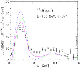
Figura 4.4: Cross section of the process ${}^{16}O(e,e^{\prime})$ at beam energy 700 MeV and electron scattering angle 32^∘. Solid line: full calculation, with inclusion of final state interaction effects. Dot-dash line: IA calculation, carried out neglecting FSI effects. Dashed line: FG model with $p_{F}=225$ MeV and $\epsilon=25$ MeV. The experimental data are from Ref.[97].

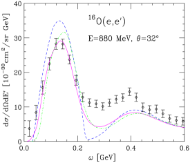
Figura 4.5: Same as in Fig. 4.4, but for beam energy 880 MeV.

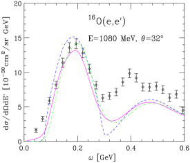
Figura 4.6: Same as in Fig. 4.4, but for beam energy 1080 MeV.

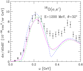
Figura 4.7: Same as in Fig. 4.4, but for beam energy 1200 MeV.

Overall, the approach described in the previous Sections, involving no adjustable parameters, provides a fairly accurate account of the measured cross sections in the region of the quasi-free peak. On the other hand, the FG model, while yielding a reasonable description at beam energies 1080 and 1200 MeV, largely overestimates the data at lower energies. The discrepancy at the top of the quasi-elastic peak turns out to be $\sim$ 25 % and $\sim$ 50 % at 880 and 700 MeV, respectively.

The results of NMBT and FG model also turn out to be sizably different in the dip region, on the right hand side of the quasi-elastic peak, while the discrepancies become less pronounced at the $\Delta$-production peak. However, it clearly appears that, independent of the employed approach and beam energy, theoretical results significantly underestimate the data at energy transfer larger than the pion production threshold.

In view of the fact that the quasi-elastic peak is correctly reproduced (within an accuracy of $\sim$ 10 %), the failure of NMBT to reproduce the data at larger $\omega$ may be ascribed to deficiencies in the description of the elementary electron-nucleon cross section. In fact, as illustrated in Fig. 4.8, the calculation of the IA cross section at the quasi-elastic and $\Delta$ production peak involves integrations of $P({\bf p},E)$ extending over regions of the $({\bf p},E)$ plane almost exactly overlapping one another.

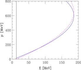
Figura 4.8: The solid and dashed lines enclose the integration regions in the $({\bf p},E)$ plane relevant to the calculation of the IA cross section at the top of the quasi-elastic and $\Delta$ production peak, respectively, for beam energy 1200 MeV and scattering angle 32^∘.

To gauge the uncertainty associated with the description of the nucleon structure functions $w_{1}^{N}$ and $w_{2}^{N}$, we have compared the electron-proton cross sections obtained from the model of Ref. [95] to the ones obtained from the model developed in Refs. [98, 99, 100] and from a global fit [101] including recent Jefferson Lab data [102]. The results of Fig. 4.9 show that at $E_{e}=1200$ MeV and $\theta=32^{\circ}$ the discrepancy between the different models is not large, being $\sim$ 15 % at the $\Delta$ production peak. It has to be noticed, however, that the models of Refs. [95, 98, 99, 100, 101] have all been obtained fitting data taken at electron beam energies larger than 2 GeV, so that their use in the kinematical regime discussed in this work involves a degree of extrapolation.

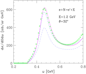
Figura 4.9: Cross section of the process $e+N\rightarrow e^{\prime}+X$ above pion production threshold, at beam energy 1200 MeV and scattering angle 32^∘. Solid line: H2 fit of Ref. [100] for $ep$ scattering; dashed line: fit of Ref. [95] for $ep$ scattering; diamonds: fit of Ref. [101] for $ep$ scattering; dot-dash line: fit of Ref. [95] for $en$ scattering.

On the other hand, the results obtained using the approach described in this paper and the nucleon structure functions of Ref. [95] are in excellent agreement with the measured $(e,e^{\prime})$ cross sections at beam energies of few GeV [83].

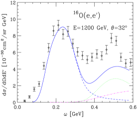
Figura 4.10: IA cross section of the process ${}^{16}O(e,e^{\prime})$ at beam energy 1200 MeV and scattering angle 32^∘. Dashed line: quasi-elastic; dots: quasi-free $\Delta$ production; dashes: nonresonant background; solid line: total. The experimental data are from Ref. [97].

Figure 4.9 also shows the prediction of the Bodek and Ritchie fit for the neutron cross section, which turns out to be much smaller than the proton one. The results of Ref. [103] suggest that extrapolating the Bodek and Ritchie fit to the low $Q^{2}$ region relevant to tha analysis of the data of Ref. [97] may lead to sizably underestimate the neutron contributions. On the other hand, the fit of Ref. [95] consistently includes both resonant and nonresonant contributions to the nuclear cross section. In this regard, it has to be pointed out that the nonresonant background is not negligible. As illustrated in Fig. 4.10, for beam energy 1200 MeV and scattering angle 32^∘ it provides $\sim$ 25 % of the cross section at energy transfer corresponding to the $\Delta$ peak.

4.5 Neutrino-nucleus cross section

The Born approximation cross section of the weak charged current process

$$\nu_{\ell}+A\rightarrow\ell^{-}+X\ ,$$ (4.26)

can be written in the form (compare to Eq. (4.2))

$$\frac{d\sigma}{d\Omega_{\ell}dE_{\ell}}=\frac{G^{2}}{32\pi^{2}}\ \frac{|{\bf k}^{\prime}|}{|{\bf k}|}\ L_{\mu\nu}W^{\mu\nu}\ ,$$ (4.27)

where $G=G_{F}\cos\theta_{C}$, $G_{F}$ and $\theta_{C}$ being Fermi’s coupling constant and Cabibbo’s angle, $E_{\ell}$ is the energy of the final state lepton and ${\bf k}$ and ${\bf k}^{\prime}$ are the neutrino and charged lepton momenta, respectively. Compared to the corresponding quantities appearing in Eq. (4.2), the tensors $L_{\mu\nu}$ and $W^{\mu\nu}$ include additional terms resulting from the presence of axial-vector components in the leptonic and hadronic currents (see, e.g., Ref. [104]).

Within the IA scheme, the cross section of Eq. (4.27) can be cast in a form similar to that obtained for the case of electron-nucleus scattering (see Eq. (4.15)). Hence, its calculation requires the nuclear spectral function and the tensor describing the weak charged current interaction of a free nucleon, $w_{N}^{\mu\nu}$. In the case of quasi-elastic scattering, neglecting the contribution associated with the pseudoscalar form factor $F_{P}$, the latter can be written in terms of the nucleon Dirac and Pauli form factors $F_{1}$ and $F_{2}$, related to the measured electric and magnetic form factors $G_{E}$ and $G_{M}$ through

$$F_{1}=\frac{1}{1-q^{2}/4m^{2}}\left(G_{E}-\frac{q^{2}}{4m^{2}}G_{M}\right)$$ (4.28)

$$F_{2}=\frac{1}{1-q^{2}/4m^{2}}\left(G_{M}-G_{E}\right)\ ,$$ (4.29)

and the axial form factor $F_{A}$.

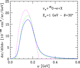
Figura 4.11: Differential cross section $d\sigma/d\Omega_{e}d\nu$ for neutrino energy $E_{\nu}=1$ GeV and electron scattering angle $\theta_{e}=30^{\circ}$. The IA results are represented by the dashed line, while the solid line corresponds to the full calculation, including the effects of FSI. The dotted line shows the prediction of the FG model with Fermi momentum $k_{F}=225$ MeV and average separation energy $\epsilon=25$ MeV.

Figure 4.11 shows the calculated cross section of the process ${}^{16}O(\nu_{e},e)$, corresponding to neutrino energy $E_{\nu}=1$ GeV and electron scattering angle $\theta_{e}=30^{\circ}$, plotted as a function of the energy transfer $\nu=E_{\nu}-E_{e}$. Numerical results have been obtained using the spectral function of Fig. 4.2 and the dipole parameterization for the form factors, with an axial mass of 1.03 GeV.

Comparison between the solid and dashed lines shows that the inclusion of FSI results in a sizable redistribution of the IA strength, leading to a quenching of the quasi-elastic peak and to the enhancement of the tails. For reference, we also show the cross section predicted by the FG model with Fermi momentum $p_{F}=225$ MeV and average separation energy $\epsilon=25$ MeV. Nuclear dynamics, neglected in the oversimplified picture in terms of noninteracting nucleons, clearly appears to play a relevant role.

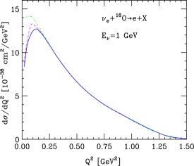
Figura 4.12: Differential cross section $d\sigma/dQ^{2}$ for neutrino energy $E=1$ GeV. The dot-dash line shows the IA results, while the solid and dashed lines have been obtained using the modified spectral function of Eq. (4.30), with and without inclusion of FSI, respectively. .

It has to be pointed out that the approach described in Chapter 3, while including dynamical correlations in the final state, does not take into account statistical correlations, leading to Pauli blocking of the phase space available to the knocked-out nucleon.

A rather crude prescription to estimate the effect of Pauli blocking amounts to modifying the spectral function through the replacement

$$P({\bf p},E)\rightarrow P({\bf p},E)\theta(|{\bf p}+{\bf q}|-{\overline{p}}_{F})$$ (4.30)

where ${\overline{p}}_{F}$ is the average nuclear Fermi momentum, defined as

$${\overline{p}}_{F}=\int d^{3}r\ \rho_{A}({\bf r})p_{F}({\bf r}),$$ (4.31)

with $p_{F}({\bf r})=(3\pi^{2}\rho_{A}({\bf r})/2)^{1/3}$, $\rho_{A}({\bf r})$ being the nuclear density distribution. For oxygen, Eq. (4.31) yields ${\overline{p}}_{F}=209$ MeV. Note that, unlike the spectral function, the quantity defined in Eq. (4.30) does not describe intrinsic properties of the target only, as it depends explicitly on the momentum transfer.

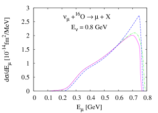
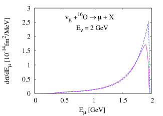
Figura 4.13: Quasi-elastic differential cross section $d\sigma/dE_{\mu}$ as a function of the scattered energy $E_{\mu}$ for the neutrino energy $E=$ 0.8 and 2.0 GeV. The solid line shows IA calculation with Pauli blocking as in Eq. (40), the dot-dash line IA calculation without Pauli blocking, and the dashed line FG model.

The effect of Pauli blocking is hardly visible in the differential cross section shown in Fig. 4.11, as the kinematical setup corresponds to $Q^{2}>0.2$ GeV² at the quasi-elastic peak. The same is true for the electron scattering cross sections discussed in the previous Section. On the other hand, this effect becomes very large at lower $Q^{2}$.

Figure 4.12 shows the calculated differential cross section $d\sigma/dQ^{2}$ for neutrino energy $E_{\nu}=1$ GeV. The dashed and dot-dash lines correspond to the IA results with and without inclusion of Pauli blocking, respectively. It clearly appears that the effect of Fermi statistic in suppressing scattering shows up at $Q^{2}<0.2$ GeV² and becomes very large at lower $Q^{2}$. The results of the full calculation, in which dynamical FSI are also included, are displayed as a full line. The results of Fig. 4.12 suggest that Pauli blocking and FSI may explain the deficit of the measured cross section at low $Q^{2}$ with respect to the predictions of Monte Carlo simulations [105].

Figure 4.13 shows the $\nu_{\mu}$-nucleus cross sections as a function of the scattered muon energy, by comparing the cross sections calculated by FG, and by the use of the spectral function with and without Pauli blocking. Figure 4.13 shows that FG yields a larger high-energy peak contribution than the other two. This is not due to the Pauli blocking, but due to the nuclear correlation effects in the spectral function: the muons tend to be scattered with a higher energy. This effect should show up in the forward angle cross section and may have a direct effect on neutrino oscillation measurements.

Capitolo 5 Low momentum transfer regime

In this chapter we focus on the nuclear matter response to weak interactions in the regime of low momentum transfer ($|{\bf q}|\sim$ 10 MeV), where the non relativistic approximation is expected to be applicable. Within this approach, the initial and final states can be obtained from NMBT, while the weak current entering the definition of the tensor $W^{\mu\nu}$ (see Eq.(4.4) and (4.27) ) is expanded in powers of $|{\bf q}|/m$. At leading order, the resulting response can be written in the simple form (compare to Eq.(2.34))

$$S({\bf q},\omega)=\frac{1}{N}\sum_{n}\langle 0|O_{{\bf q}}^{\dagger}|n\rangle\langle n|O_{{\bf q}}|0\rangle\delta(\omega+E_{0}-E_{n})\ .$$ (5.1)

where, in the case of charged current interactions, $O_{{\bf q}}$ is the operator corresponding to Fermi or Gamow-Teller transitions.

The calculation of the nuclear matter response has been carried out using CBF states, obtained from the states of the noninteracting system trough the transformation (2.2), and the two-body cluster approximation for the weak transition matrix elements (see Chapter 2). The effect of long range correlations, which are known to play a critical role at low momentum transfer, has been also included in our scheme in a fully consistent fashion, using the effective interaction defined in Chapter 2 and the Tamm-Dancoff (TD) approximation [46, 106]. We will restrict our discussion to the case of Fermi transitions. The extension to Gamow-Teller transitions is trivial.

5.1 Non relativistic reduction of the weak charged current

The starting point of our calculation is the non relativistic reduction of the weak charged current operator. Basically, one needs to expand in powers of $|{\bf q}|/m$ the matrix elements

$$\langle{\bf p}^{\prime}|J_{\mu V}^{+}|{\bf p}\rangle = \overline{u}({\bf p}^{\prime},s^{\prime}\eta^{\prime})\Gamma_{\mu}u({\bf p},s)\ \eta_{t^{\prime}}^{\dagger}\tau^{+}\eta_{t}$$

$$\langle{\bf p}^{\prime}|J_{\mu A}^{+}|{\bf p}\rangle = \overline{u}({\bf p}^{\prime},s^{\prime})\Gamma_{\mu A}\tau^{+}u({\bf p},s)\ \eta_{t^{\prime}}^{\dagger}\tau^{+}\eta_{t}\ ,$$ (5.2)

where

$$\Gamma^{\mu}=\gamma^{\mu}F_{1}+i\sigma^{\mu\nu}q_{\nu}\frac{F_{2}}{2m}+q^{\mu}F_{S}\ ,$$ (5.3)

with $\sigma^{\mu\nu}=i[\gamma_{\mu},\gamma_{\nu}]/2$, $\gamma^{\mu}$ being the Dirac matrices, and

$$\Gamma^{\mu}_{A}=\gamma^{\mu}\gamma^{5}F_{A}+q^{\mu}\gamma^{5}F_{P}+i\gamma^{5}\sigma^{\mu\nu}q_{\nu}F_{T}\ .$$ (5.4)

In the above equations, $\gamma^{5}=i\gamma^{0}\gamma^{1}\gamma^{2}\gamma^{3}$, $u({\bf p},s)$ is the spinor describing a Dirac fermion with momentum ${\bf p}$ and spin polarization $s$, $\eta_{t}$ is the Pauli spinor specifying the isospin state of the nucleon, $\tau^{+}=(\tau^{1}+i\tau^{2})/2$ is the isospin raising operator and the form factors $F_{1}$, $F_{2}$, $F_{S}$, $F_{A}$, $F_{P}$ and $F_{T}$ are functions of the squared four momentum transfer $q^{2}$.

From the definition

$$u({\bf p},s)=N_{\bf p}\left(\begin{array}[]{c}\chi_{s}\\ \\ \frac{{\mbox{\boldmath{$\sigma$}}}\cdot\textbf{p}}{E_{\bf p}+m}\chi_{s}\end{array}\right)\ ,$$ (5.5)

where $N_{{\bf p}}$ is a normalization constant and $\chi_{s}$ is a Pauli spinor, it follows that, to zero-th order in $|{\bf q}|/m$, we can write

$$\langle{\bf p}^{\prime}|J_{0V}^{+}(0)|{\bf p}\rangle\simeq F_{1}(0)\ \chi_{s^{\prime}}^{\dagger}\chi_{s}\ \eta_{t^{\prime}}^{\dagger}\tau^{+}\eta_{t}\ .$$ (5.6)

Due to the antidiagonal structure of the matrix $\gamma^{5}$, the corresponding matrix element of the axial vector current, $\langle{\bf p}^{\prime}|J_{0A}^{+}(0)|{\bf p}\rangle$, does not have any zero-th order contributions.

In conclusion, denoting $g_{V}=F_{1}(0)$ the non relativistic reduction amounts to making the replacement

$$\langle{\bf r}_{i}^{\prime}|J^{+}_{0}V({\bf q})|{\bf r}_{i}\rangle\rightarrow\ O^{F}_{i}({\bf q})=g_{V}\delta({\bf r}_{i}-{\bf r}_{i}^{\prime})\ \ {\rm e}^{i{\bf q}{\bf r}_{i}}\tau_{i}^{+}\ ,$$ (5.7)

which defines the Fermi transition operator $O^{F}_{i}({\bf q})$ in coordinate space.

The axial part of the current contributes through the $\mu=i=1,2,3$ components

$$\langle{\bf p}^{\prime}|{\bf J}_{A}|{\bf p}\rangle = \overline{u}({\bf p}^{\prime},s^{\prime})[F_{A}{\mbox{\boldmath{$\gamma$}}}\gamma_{5}+F_{P}\gamma_{0}{\bf q}\gamma_{5}]u({\bf p},s\ \eta_{t^{\prime}}\tau^{+}\eta_{t}$$ (5.8)

$$= u^{\dagger}({\bf p}^{\prime},s^{\prime})[F_{A}\gamma_{0}{\mbox{\boldmath{$\gamma$}}}\gamma_{5}+F_{P}\gamma_{0}{\bf q}\gamma_{5}]\tau^{+}u({\bf p},s)\ \eta_{t^{\prime}}\tau^{+}\eta_{t}\ .$$

In the above equation, the zero-th order term proportional to $F_{P}$ vanishes because $\gamma_{0}\gamma_{5}$ is antidiagonal. As for the term proportional to $F_{A}$ we find instead

$$\gamma_{0}{\mbox{\boldmath{$\gamma$}}}\gamma_{5}=\left(\begin{array}[]{cc}I&0\\ 0&-I\end{array}\right)\left(\begin{array}[]{cc}0&{\mbox{\boldmath{$\sigma$}}}\\ -{\mbox{\boldmath{$\sigma$}}}&0\end{array}\right)\left(\begin{array}[]{cc}0&I\\ I&0\end{array}\right)=\left(\begin{array}[]{cc}{\mbox{\boldmath{$\sigma$}}}&0\\ 0&{\mbox{\boldmath{$\sigma$}}}\end{array}\right)\ .$$ (5.9)

Finally, the vector part of ${\bf J}^{+}$ does not contribute at zero-th order.

Making use of Eq.(5.9), we can then write

$$\langle{\bf r}_{i}^{\prime}|{\bf J}^{+}_{0}({\bf q})|{\bf r}_{i}\rangle\rightarrow{\bf O}^{GT}_{i}({\bf q})=g_{A}\delta({\bf r}_{i}-{\bf r}_{i}^{\prime})\ {\rm e}^{i{\bf q}{\bf r}_{i}}{\mbox{\boldmath{$\sigma$}}}_{i}\tau_{i}^{+}\ ,$$ (5.10)

with $g_{A}=F_{A}(0)$, which defines the operator inducing Gamow-Teller transitions.

5.2 Correlated matrix elements and effective operators

Using correlated states implies severe difficulties in the explicit calculation of the weak matrix element. In the FG model, the nuclear response is non vanishing only when the final nuclear state differs from the initial state for the presence of a particle excited outside the Fermi sea and a hole in the Fermi sea. In the presence of correlations, which can induce virtual nucleon-nucleon scattering processes leading to excitation of nucleons to states outside the Fermi sea, more complex scenarios must also be considered. For example, if the initial state has a two particle-two hole component, the final state can be a three particle-three hole state or, if the probe interacts with an excited nucleon, a two particle-two hole state.

In the following we will consider only the dominant transition, between the correlated ground state and a correlated one particle-one hole ($ph$) state. The corresponding Weak matrix element can be written

$$M_{ph}=\frac{\langle ph|F^{\dagger}OF|0\rangle}{\langle ph|F^{\dagger}F|ph\rangle^{\frac{1}{2}}\langle 0|F^{\dagger}F|0\rangle^{\frac{1}{2}}}\ ,$$ (5.11)

where $F$ is the correlation operator defined in Eq.(2.3). Here the kets $|0\rangle$ and $|ph\rangle$ correspond to the ground and one particle-one hole Fermi Gas states, respectively, and $O=\sum_{i}O_{i}$, $O_{i}$ being the Fermi or the Gamow-Teller transition operator (see Eqs.(5.7)) and (5.10)).

In calculating the weak matrix element, we will use the two-body cluster approximation discussed in Chapter 2. Let us define

$$g_{ij}=f_{ij}-1\ ,$$ (5.12)

with $f_{ij}$ defined as in Eq,(2.5). Note the the $g_{ij}$ is short ranged, and therefore its matrix elements are small.

At two-body level, the cluster expansion Eq.(5.11) yields

$$\langle ph|F^{\dagger}OF|0\rangle \simeq \langle ph|(1+\sum_{j>i}g_{ij})O(1+\sum_{j>i}g_{ij})|0\rangle$$ (5.13)

$$= N\langle ph|O_{1}|0\rangle+\frac{N(N-1)}{2}\langle ph|\{O_{1}+O_{2},g_{12}\}|0\rangle$$

$$+ \frac{N(N-1)}{2}\langle ph|g_{12}(O_{1}+O_{2})g_{12}|0\rangle\ ,$$

where $\{A,B\}=AB+BA$. The above equation, suggest the definition of an effective operator $O^{eff}_{12}$, acting on Fermi Gas states, reminiscent of the effective interaction of Chapter 2. From

$$\langle ph|F^{\dagger}OF|0\rangle=\langle ph|O^{eff}|0\rangle.$$ (5.14)

it follows that, at the two-body cluster level (compare to Eq.(5.13))

$$\frac{1}{N}O^{eff}_{12}=O_{1}+\frac{N-1}{2}\{O_{1}+O_{2}.g_{12}\}+\frac{N-1}{2}[g_{12}(O_{1}+O_{2})g_{12}]\ .$$ (5.15)

Note that the $O^{eff}$ is a two-body operator, as it includes screening effects arising from nucleon-nucleon correlations.

Replacing Eq.(5.13) into Eq.(5.11) leads to

$$M_{ph}\simeq N_{1}+N_{2}+N_{3}$$ (5.16)

where

$$N_{1} = N\langle ph|O_{1}|0\rangle\ ,$$ (5.17)

$$N_{2} = \frac{N(N-1)}{2}\langle ph|\{O_{1}+O_{2},g_{12}\}|0\rangle\ ,$$ (5.18)

$$N_{3} = \frac{N(N-1)}{2}\langle ph|g_{12}(O_{1}+O_{2})g_{12}|0\rangle\ .$$ (5.19)

The wave function of the FG ground state $\Psi_{0}(R)=\langle R|0\rangle$ can be written as a determinant according to

$$\Psi_{0}(X)=\frac{1}{\sqrt{N!}}\left|\begin{array}[]{ccc}\phi_{1}(1)&\cdots&\phi_{N}(1)\\ \vdots&\ddots&\vdots\\ \phi_{1}(N)&\cdots&\phi_{N}(N)\\ \end{array}\right|\ ,$$ (5.20)

where $\phi_{m}(n)$ is the wave function describing the n-th particle in the state $m$, with momentum ${\bf k}_{m}$ and spin and isospin projections $s_{m}$ and $t_{m}$, respectively

$$\phi_{m}(n)=\frac{1}{\sqrt{V}}{\rm e}^{i{\bf k}_{m}{\bf r}_{n}}\chi_{s_{m}}\eta_{t_{m}}\ .$$ (5.21)

One particle-one hole states, and the corresponding wave functions $\Psi_{ph}(R)=\langle 0|ph\rangle$, can be built from the ground state through

$$|ph\rangle=a^{\dagger}_{p}a_{h}|0\rangle$$ (5.22)

using Eq.(5.20).

As $g_{ij}$ is a two-body operator, it turns out to be convenient rewriting the ground and one particle-one hole wave functions, $\Psi_{0}(R)$ and $\Psi_{ph}(R)$, in the form (see Eq.(5.20))

$$\Psi_{0}(R) = \frac{1}{\sqrt{N(N-1)}}\sum_{\alpha\beta}(-1)^{n_{\alpha}+n_{\beta}}\phi_{\alpha}(1)\phi_{\beta}(2)\Phi_{\gamma\neq\alpha,\beta}(3,\cdots,N),$$ (5.23)

$$\Psi_{ph}(R) = \frac{1}{\sqrt{N(N-1)}}\left\{\sum_{\alpha\neq h}\sum_{\beta\neq\alpha,h}(-1)^{n_{\alpha}+n_{\beta}}\right.\phi_{\alpha}(1)\phi_{\beta}(2)\Phi_{p,\gamma\neq\alpha,\beta,h}(3,\cdots,N)$$

$$+ \sum_{\alpha\neq h}(-1)^{n_{\alpha}+n_{h}}\phi_{\alpha}(1)\phi_{p}(2)\Phi_{\gamma\neq\alpha,h}(3\cdots N)$$

$$+ \left.\sum_{\alpha\neq h}(-1)^{n_{\alpha}+n_{h}+1}\phi_{\alpha}(2)\phi_{p}(1)\Phi_{\gamma\neq\alpha,h}(3,\cdots N)\right\}\ ,$$

where $\Phi_{p,\gamma\neq\alpha,\beta}(3,\cdots,N)$ denotes the wave function of a $N-2$-particle system, with a particle in the state $p$ and holes in the state $\gamma\neq\alpha,\ \beta$.

The (N-2)-particle wave functions satisfy the following orthonormalization relations

$$\int\ d^{3}r_{3}\cdots d^{3}r_{n}\ \Phi^{\dagger}_{\gamma\neq\alpha,\beta}(3,\cdots,N)\Phi_{p,\gamma\neq\alpha^{\prime},\beta^{\prime},h}(3,\cdots,N)=0\ ,$$ (5.24)

$$\int\ d^{3}r_{3}\cdots d^{3}r_{n}\Phi^{\dagger}_{\gamma\neq\alpha\beta}(3,\cdots,N)\Phi_{\gamma\neq\alpha^{\prime},h}(3,\cdots,N)=\delta_{\alpha\alpha^{\prime}}\ \delta_{\beta h}\ .$$ (5.25)

With the help of the above equations, the weak matrix element can be reduced to an integral over the coordinates of two particles.

The next section will be devoted to the details of the calculation of the Fermi transition matrix element. We will start writing it as a sum of contributions corresponding to the physical processes schematically represented by the diagrams of Figs. 5.1-5.5. The different contributions will be labeled by three indices

• the first index, $B$ or $C$, denotes the order (first and second, respectively) in the correlation $g$;

• the value of the second index, 1 or 2, indicates that the Fermi operator acts on particle 1 (any nucleon inside the Fermi-sea in the initial state) or on particle 2 (the active particle, carrying momentum ${\bf h}$ and spin projection $\sigma_{h}$ in the ground state);

• the third index specifies the direct ($d$) and exchange ($e$) contributions to the matrix elements. Note that exchange terms carry an additional minus sign.

As the Fermi operator involves the isospin raising operator, the only non vanishing matrix elements are those in which the particle excited outside the Fermi-sea is a proton and the active particle in the initial state is a neutron.

5.2.1 Fermi Transition

We will now discuss the explicit calculation of the weak matrix element. Since the corresponding operator does not induce spin transitions, all contributions to the matrix element involve a Kronecker delta expressing the condition $\sigma_{p}=\sigma_{h}$, where $\sigma_{p}$ and $\sigma_{h}$ are the spin projections of the particle and hole states, respectively. In order to simplify the notation, this factor will be omitted.

From Eq.(5.17) we obtain

$$N_{1} = N\langle ph|O_{1}|0\rangle=\rho\int d^{3}r_{1}e^{-i{\bf p}{\bf r}_{1}}e^{i{\bf q}{\bf r}_{1}}e^{i{\bf h}{\bf r}_{1}}\chi^{\dagger}_{p}\chi_{h}\eta^{\dagger}_{p}\tau^{+}\eta_{h}$$ (5.26)

$$= \rho\ (2\pi)^{3}\delta^{(3)}({\bf p}-{\bf h}-{\bf q})\ ,$$

where $\chi_{p(h)}=\chi_{\sigma_{p(h)}}$ and $\eta_{p(h)}=\eta_{\tau_{p(h)}}$.

Figura 5.1: Diagram associated with the contribution $N_{1}$ (see Eq.(5.17)).

The above equation shows that $N_{1}$, the leading term of the expansion, is just the Fermi transition matrix element in the absence of correlations.

Io order to write down the complete expression of $N_{2}$, let us consider the matrix element

$$B1 = \frac{N(N-1)}{2}\int dR\Psi^{\dagger}_{ph}\{O_{1},g_{12}\}\Psi_{0}(R)$$

$$= \frac{1}{2}\sum_{\alpha}\int d^{3}r_{1}d^{3}r_{2}[\phi_{\alpha}(1)\phi_{p}(2)-\phi_{p}(1)\phi_{\alpha}(2)]\{O_{1},g_{12}\}\phi_{\alpha}(1)\phi_{h}(2)\ ,$$

in which we have used Eqs.(5.23)-(5.2) and the sum is extended over the Fermi sea. The right hand side of Eq.(5.2.1) has both direct and exchange contributions; for the direct term we can write

$$B1d = \frac{1}{2}\frac{1}{V^{2}}\sum_{\alpha}\sum_{n}\int d^{3}r_{1}d^{3}r_{2}e^{-i({\bf k}_{\alpha}{\bf r}_{1}+{\bf p}{\bf r}_{2})}e^{i{\bf q}{\bf r}}e^{i({\bf k}_{\alpha}{\bf r}_{1}+{\bf h}{\bf r}_{2})}g_{n}(r)$$ (5.28)

$$\times \langle\alpha p|\{\tau_{1}^{+},O^{12}_{n}\}|\alpha h\rangle\ ,$$

where the $g_{n}(r)$ are the radial functions entering the definition of $g_{12}$ and $r=|{\bf r}_{1}-{\bf r}_{2}|$. From now on, the ket $|\alpha\beta\rangle$ indicates a state in which particles 1 and 2 have spin-isospin $\alpha$ and $\beta$, respectively. Carrying out the change of variables

$$\left\{\begin{array}[]{l}{\bf r}={\bf r}_{1}-{\bf r}_{2}\\ \\ {\bf R}=({\bf r}_{1}+{\bf r}_{2})/2\ ,\end{array}\right.$$ (5.29)

and integrating over ${\bf R}$ we obtain

$$B1d=\frac{\rho}{4V}(2\pi)^{3}\delta^{(3)}({\bf p}-{\bf q}-{\bf h})\sum_{\sigma_{\alpha},\tau_{\alpha}}\sum_{n}\int d^{3}re^{i{\bf q}{\bf r}}g_{n}(r)\langle\alpha p|\{\tau_{1}^{+},O^{12}_{n}\}|\alpha h\rangle,$$ (5.30)

where we have used

$$\sum_{\alpha}\rightarrow\sum_{k_{\alpha},\sigma_{\alpha},\tau_{\alpha}}\rightarrow\frac{N}{4}\sum_{\sigma_{\alpha},\tau_{\alpha}}\ .$$ (5.31)

Let us now focus on the spin-isospin matrix element. From the definition of the six operators $O^{12}_{n}$ (1.16) and

$$\langle\alpha|\tau^{+}|\alpha\rangle = 0\ ,$$

$$\sum_{\sigma_{\alpha}}\langle\alpha p|{\mbox{\boldmath{$\sigma$}}}_{1}{\mbox{\boldmath{$\sigma$}}}_{2}|\alpha h\rangle = 0\ ,$$

$$\sum_{\sigma_{\alpha}}\langle\alpha p|S_{12}|\alpha h\rangle = 0\ ,$$

it follows that the only non-vanishing contribution is given by

$$\sum_{\sigma_{\alpha},\tau_{\alpha}}\langle\alpha p|\{\tau_{1}^{+},{\mbox{\boldmath{$\tau$}}}_{1}{\mbox{\boldmath{$\tau$}}}_{2}\}|\alpha h\rangle=8\ .$$ (5.33)

Note that the previous result was obtained exploiting the anticommutator

$$\{\tau_{1}^{+},{\mbox{\boldmath{$\tau$}}}_{1}{\mbox{\boldmath{$\tau$}}}_{2}\}=2\tau_{2}^{+}.$$ (5.34)

The final expression of $B1d$ turns out to be

$$B1d=\frac{\rho}{4V}(2\pi)^{3}\delta^{(3)}({\bf p}-{\bf q}-{\bf h})\ 8\int d^{3}re^{i{\bf q}{\bf r}}\ g_{2}(r).$$ (5.35)

Figura 5.2: Diagram associated with the contribution $B1d$ (see Eq.(5.28)).

Let us now consider the exchange term. Performing again the change of variables of Eq.(5.29), we find the expression

$$B1e=\frac{1}{2}\frac{1}{V^{2}}(2\pi)^{3}\delta^{(3)}({\bf p}-{\bf q}-{\bf h})\sum_{\alpha,n}\int d^{3}re^{-i({\bf h}+{\bf k}_{\alpha}){\bf r}}g_{n}(r)\langle p\alpha|\{\tau_{1}^{+},O^{12}_{n}\}|\alpha h\rangle\ ,$$ (5.36)

which, after summing over $k_{\alpha}$, becomes

$$B1e=\frac{\rho}{4V}(2\pi)^{3}\delta^{(3)}({\bf p}-{\bf q}-{\bf h})\sum_{\sigma_{\alpha},\tau_{\alpha},n}\int d^{3}re^{-i{\bf h}{\bf r}}g_{n}(r)\ell(k_{F}r)\langle p\alpha|\{\tau_{1}^{+},O^{12}_{n}\}|\alpha h\rangle\ ,$$ (5.37)

where

$$\ell(k_{F}r)=\frac{4}{\rho}\int_{0}^{k_{F}}\frac{d^{3}k}{(2\pi)^{3}}e^{i{\bf k}{\bf r}}\\ =3\ \frac{\sin(k_{F}r)-(k_{F}r)\cos(k_{F}r)}{(k_{F}r)^{3}}\ ,$$ (5.38)

is the Slater function.

For the spin-isospin matrix element, using the completeness relation

$$\sum_{\sigma_{\alpha},\tau_{\alpha}}|\alpha\rangle\langle\alpha|=1\ .$$ (5.39)

we can write:

$$\sum_{\sigma_{\alpha},\tau_{\alpha}}\langle p\alpha|\{1,\tau_{1}^{+}\}|\alpha h\rangle=2\ ,$$

$$\sum_{\sigma_{\alpha},\tau_{\alpha}}\langle p\alpha|\{{\mbox{\boldmath{$\tau$}}}_{1}{\mbox{\boldmath{$\tau$}}}_{2},\tau_{1}^{+}\}|\alpha h\rangle=2\ ,$$

$$\sum_{\sigma_{\alpha},\tau_{\alpha}}\langle p\alpha|\{{\mbox{\boldmath{$\sigma$}}}_{1}{\mbox{\boldmath{$\sigma$}}}_{2},\tau_{1}^{+}\}|\alpha h\rangle=6\ ,$$

$$\sum_{\sigma_{\alpha},\tau_{\alpha}}\langle p\alpha|\{{\mbox{\boldmath{$\tau$}}}_{1}{\mbox{\boldmath{$\tau$}}}_{2}{\mbox{\boldmath{$\sigma$}}}_{1}{\mbox{\boldmath{$\sigma$}}}_{2},\tau_{1}^{+}\}|\alpha h\rangle=6\ ,$$

$$\sum_{\sigma_{\alpha},\tau_{\alpha}}\langle p\alpha|\{S_{12},\tau_{1}^{+}\}|\alpha h\rangle=0\ ,$$

$$\sum_{\sigma_{\alpha},\tau_{\alpha}}\langle p\alpha|\{S_{12}{\mbox{\boldmath{$\tau$}}}_{1}{\mbox{\boldmath{$\tau$}}}_{2},\tau_{1}^{+}\}|\alpha h\rangle=0\ .$$

Collecting all the above results we finally obtain

$$B1e=\frac{\rho}{4V}(2\pi)^{3}\delta^{(3)}({\bf p}-{\bf q}-{\bf h})\int d^{3}re^{-i{\bf h}{\bf r}}\ell(k_{F}r)[2g_{1}+2g_{2}+6g_{3}+6g_{4}].$$ (5.40)

Figura 5.3: Diagram associated with the contribution $B1e$ (see Eq.(5.40)).

Note that, in order to simplify the notation, in the above equation and in the rest of this Section the functional dependence of the $g_{n}$’s on $r$ is omitted.

The contributions $B2d$ and $B2e$ can be obtained from $B1d$ and $B1e$ through the substitution

$$e^{i{\bf q}{\bf r}_{1}}\tau_{1}^{+}\rightarrow e^{i{\bf q}{\bf r}_{2}}\tau_{2}^{+}\ .$$ (5.41)

For the direct term, $B2d$, we find

$$B2d=\frac{\rho}{4V}(2\pi)^{3}\delta^{(3)}({\bf p}-{\bf q}-{\bf h})\ 8\int d^{3}r\ g_{1}(r)\ ,$$ (5.42)

Figura 5.4: Diagram associated with the contribution $B2d$ (see Eq.(5.42)).

while the exchange term, $B2e$, reads

$$B2e=\frac{\rho}{4V}(2\pi)^{3}\delta^{(3)}({\bf p}-{\bf q}-{\bf h})\int d^{3}re^{-i{\bf p}{\bf r}}\ell(k_{F}r)[2g_{1}+2g_{2}+6g_{3}+6g_{4}]\ .$$ (5.43)

The contributions of Eq.(5.19), $N_{3}$, can again be obtained from the corresponding contributions of Eq.(5.17), $N_{1}$, through the substitution

$$\sum_{n}g_{n}\langle\alpha^{\prime}\beta^{\prime}|\{O_{n}^{12},\tau^{+}_{i}\}|\alpha\beta\rangle\rightarrow\sum_{n,n^{\prime}}g_{n}g_{n^{\prime}}\langle\alpha^{\prime}\beta^{\prime}|O_{n}^{12}\tau_{i}^{+}O_{n^{\prime}}^{12}|\alpha\beta\rangle\ .$$ (5.44)

As the six operators $O_{n}^{12}$ form an algebra (see Appendix A), we can write

$$O_{n}^{12}O_{m}^{12}=\sum_{r}K_{nmr}O_{r}^{12}\ .$$ (5.45)

Exploiting this property, the product of two or more operators can be rewritten as a linear combination of the six operators. We will also make use of the following relations

$$({\mbox{\boldmath{$\sigma$}}}{\bf A})({\mbox{\boldmath{$\sigma$}}}{\bf B}) = ({\bf AB})+i{\mbox{\boldmath{$\sigma$}}}({\bf A}\times{\bf B}),$$ (5.46)

$$({\mbox{\boldmath{$\sigma$}}}_{1}{\mbox{\boldmath{$\sigma$}}}_{2})^{2} = 3-2({\mbox{\boldmath{$\sigma$}}}_{1}{\mbox{\boldmath{$\sigma$}}}_{2}),$$ (5.47)

$$S_{12}({\mbox{\boldmath{$\sigma$}}}_{1}{\mbox{\boldmath{$\sigma$}}}_{2}) = ({\mbox{\boldmath{$\sigma$}}}_{1}{\mbox{\boldmath{$\sigma$}}}_{2})S_{12}=S_{12},$$ (5.48)

$$S_{12}^{2} = 6+2({\mbox{\boldmath{$\sigma$}}}_{1}{\mbox{\boldmath{$\sigma$}}}_{2})-2S_{12}.$$ (5.49)

The first equation of the above group follows from the properties of the Pauli matrices. The second can be obtained directly from the first, while the third and fourth can be easily derived writing the tensor $S_{12}$ in the form:

$$S_{12}=\sum_{ij}(3\hat{r}_{i}\hat{r}_{j}-\delta_{ij})\sigma_{1}^{i}\sigma_{2}^{j},$$ (5.50)

where $\hat{r}$ is the unit vector in the direction of ${\bf r}$.

Figura 5.5: Diagram associated with the contribution $C1d$ (see Eq.(5.51)).

Using Eqs.(5.46)-(5.49) we find

$$C1d = \frac{\rho}{4V}(2\pi)^{3}\delta^{(3)}({\bf p}-{\bf q}-{\bf h})$$ (5.51)

$$\ \ \times\int d^{3}re^{i{\bf q}{\bf r}}[8g_{1}g_{2}+8g_{2}^{2}+24g_{4}^{2}+48g_{6}^{2}+24g_{3}g_{4}+48g_{5}g_{6}]\ ,$$

and

$$C1e = \frac{\rho}{4V}(2\pi)^{3}\delta^{(3)}({\bf p}-{\bf q}-{\bf h})\int d^{3}re^{-i{\bf h}{\bf r}}\ell(k_{F}r)[g_{1}^{2}+2g_{1}g_{2}+6g_{1}g_{3}+6g_{1}g_{4}$$ (5.52)

$$+ g_{2}^{2}-3g_{3}^{2}-3g_{4}^{2}+12g_{5}^{2}+12g_{6}^{2}+6g_{2}g_{3}+6g_{2}g_{4}-6g_{3}g_{4}+24g_{5}g_{6}]\ .$$

Following the same procedure and using the substitution (5.41) we also obtain

$$C2d=\frac{\rho}{4V}(2\pi)^{3}\delta^{(3)}({\bf p}-{\bf q}-{\bf h})\int\ d^{3}r[8g_{1}^{2}-4g_{2}^{2}+12g_{3}^{2}-12g_{4}^{2}+24g_{5}^{2}-24g_{6}^{2}]\,$$ (5.53)

$$C2e = \frac{\rho}{4V}(2\pi)^{3}\delta^{(3)}({\bf p}-{\bf q}-{\bf h})\int\ d^{3}re^{-i{\bf p}{\bf r}}[2g_{1}^{2}+2g_{1}g_{2}+6g_{1}g_{3}+6g_{1}g_{4}$$ (5.54)

$$+g_{2}^{2}-3g_{3}^{2}+12g_{5}^{2}+12g_{6}^{2}+6g_{2}g_{3}+6g_{2}g_{4}-6g_{3}g_{4}+24g_{5}g_{6}].$$

5.3 Calculation of the response

In the previous Sections, we have defined all the ingredients needed to obtain the weak response of nuclear matter in the one particle-one hole channel. For reasons that will become apparent in the next Section, devoted to the discussion of the TD approximation, numerical calculations have been carried out in a cubic box of finite volume $L^{3}$, using a discrete set of one particle one-hole states. Within this scheme, the allowed nucleon momenta ${\bf k}$ are given by

$${\bf k}=\frac{2\pi}{L}(n^{x}{\hat{x}}+n^{y}{\hat{y}}+n^{z}{\hat{z}})\ ,$$ (5.55)

where $n^{x},\ n^{y},\ n^{z}=0,\ \pm 1,\ \pm 2,\ \ldots$ and ${\hat{x}},\ {\hat{y}}$ and ${\hat{z}}$ are unit vectors along the directions of the cartesian axes.

As we are interested in the low momentum transfer regime ($|{\bf q}|\ll k_{F}$), we determine the size of the normalization box by requiring that ${\bf q}$ be on the lattice, i.e. that

$${\bf q}=\frac{2\pi}{L}(n_{q}^{x}{\hat{x}}+n_{q}^{y}{\hat{y}}+n_{q}^{z}{\hat{z}})\ .$$ (5.56)

For fixed momentum transfer, i.e. for fixed $n_{q}^{x},\ n_{q}^{y},\ n_{q}^{z}$ and $|{\bf q}|$, the above equation yields

$$L=2\pi\frac{n_{q}}{|{\bf q}|}\ ,$$ (5.57)

with

$$n_{q}=\sqrt{(n_{q}^{x})^{2}+(n_{q}^{y})^{2}+(n_{q}^{z})^{2}}\ .$$ (5.58)

Obviously, in the $L\rightarrow\infty$ limit our procedure must reproduce the results obtained working with a continuum set of one particle-one hole states.

Let us rewrite the definition of the response using the effective operator, defined as in Eq.(5.14), associated with Fermi transitions

$$S_{F}({\bf q},\omega)=\frac{2}{N}\sum_{|{\bf h}|\leq k_{F},|{\bf p}|\geq k_{F}}|\langle ph|O_{eff}^{F}({\bf q})|0\rangle|^{2}\delta(\omega+E_{0}-E_{ph})\delta({\bf p}-{\bf h}-{\bf q})\ .$$ (5.59)

Note that the factor $2$ in the right hand side of the above equation comes from the sum over the particle and hole spin projections.

For the sake of illustration, we will first consider the noninteracting FG model. In this case we find

$$|M_{ph}({\bf q})|^{2}=|\langle ph|O_{eff}^{F}({\bf q})|0\rangle|^{2}\rightarrow|\langle ph|O^{F}({\bf q})|0\rangle|^{2}\ =1\ ,$$ (5.60)

and

$$E_{ph}-E_{0}=\omega_{p}-\omega_{h}=\omega_{ph}\ ,$$ (5.61)

with

$$\omega_{k}=\frac{|{\bf k}|^{2}}{2m}\ .$$ (5.62)

The sum appearing in Eq.(5.59) is extended to all lattice momenta

$${\bf h}_{i}=\frac{2\pi}{L}(n^{x}_{i}{\hat{x}}+n^{y}_{i}{\hat{y}}+n^{z}_{i}{\hat{z}})$$ (5.63)

such that $|{\bf h}_{i}|\leq k_{F}$ and $|{\bf h}_{i}+{\bf q}|\geq k_{F}$, with ${\bf q}$ given by Eq.(5.56).

Obviously, the response obtained from the discrete set of final states consists of a collection of delta function peaks located at $\omega=\omega_{i}=\omega_{|{\bf h}_{i}+{\bf q}|}-\omega_{h_{i}}$. A smooth function of $\omega$ has been obtained using a finite width gaussian representation of the energy conserving $\delta$ function, i.e. replacing

$$\delta(\omega-\omega_{i})\rightarrow\frac{1}{\sigma\sqrt{\pi}}\ {\rm exp}\{-[(\omega-\omega_{i})/\sigma]^{2}\}\ .$$ (5.64)

For sufficiently small values of $\sigma$, the results obtained using this procedure become independent of $\sigma$.

In Fig. 5.6 the FG response at $|{\bf q}|=0.3\ {\rm fm}^{-1}$, obtained from an analytical calculation using a continuum set of one particle-one hole states, is compared to that resulting from the above procedure with $(n_{q}^{x},\ n_{q}^{y},\ n_{q}^{z})\equiv(1,2,3)$. This choice corresponds to a normalization box of linear dimension $L=78\ {\rm fm}$, containing $\sim$ 78400 nucleons. The corresponding number of one particle-one hole states in the basis is $\sim$ 3000. It clearly appears that the basis is large enough to reproduce the results obtained in the continuum limit.

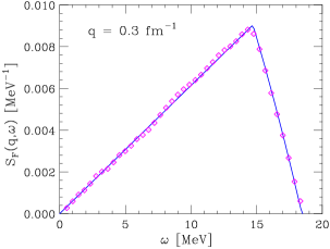
Figura 5.6: Comparison between the FG response at $|{\bf q}|=0.3\ {\rm fm}^{-1}$ evaluated in a cubic box of side $L=78\ {\rm fm}$ using a basis of $\sim$ 3000 states (diamonds) and that resulting from an analytical calculation using a continuum set of one particle-one hole states (solid line).

5.4 Correlated Hatree-Fock approximation

The inclusion of interaction leads to sizable modifications of the FG response. Correlation effects in the transition matrix elements, taken into account through the use of the effective operator, produce a quenching of the Fermi transition matrix elements of $\sim$ 15 %, largely independent of the hole momentum, as illustrated in Fig. 5.7. Note that the effect on the response is larger, as its definition involves the transition probabilities, i.e. the squared matrix elements. This feature is apparent in Fig. 5.8, where the FG response, represented by diamonds, is compared to that obtained using the effective operator in the calculation of $M_{ph}$ and the FG spectrum of Eq.(5.62), represented by crosses.

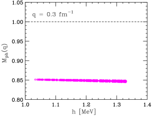
Figura 5.7: Fermi transition matrix element at $|{\bf q}|=0.3\ {\rm fm}^{-1}$ as a function of the magnitude of hole momentum $|{\bf h}|$. The dashed horizontal line corresponds to the result of the FG model.

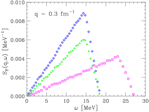
Figura 5.8: Nuclear matter response at $|{\bf q}|=0.3\ {\rm fm}^{-1}$. Diamonds: FG model. Crosses: results obtained using the effective operator in the calculation of $M_{ph}$ and the FG spectrum of Eq.(5.62). Squares: correlated HF approximation described in the text.

An even larger modification is produced by interaction effects on the single particle energies. Corrections to the kinetic energy spectrum (5.62) have been calculated within the Hartree-Fock (HF) approximation, using the CBF effective interaction discussed in Chapter 2 (see Eq.(2.63)). Replacing the single particle energies of Eq.(5.62) with the HF energies, shown by the solid line in Fig. 2.5, leads to a sizable broadening of $\omega$ region corresponding to non-vanishing response.

The squares of Fig. 5.8 show the response evaluated within the correlated HF approximation , i.e. using the CBF effective operator and the HF spectrum obtained from the CBF effective interaction, at $|{\bf q}|=0.3\ {\rm fm}^{-1}$. Comparison with the diamonds and the crosses shows that using the HF spectrum leads to an increase of the upper limit of the energy transfer $\omega$ from $\sim$ 18 MeV to $\sim$ 27 MeV.

In Figs. 5.9-5.10 the comparison between FG model and correlated HF approximation is extended to larger values of the momentum transfer $|{\bf q}|=1.8,\ {\rm and}\ 3.0\ {\rm fm}^{-1}$, corresponding to the regions $|{\bf q}|\geq k_{F}$ and $|{\bf q}|\geq 2k_{F}$, respectively. In the case $|{\bf q}|=1.8,\ {\rm fm}^{-1}$ we have used a box of side $L=\sim 47\ {\rm fm}$, corresponding to a basis of $\sim 3900$ states, while the calculation at $|{\bf q}|=3.0,\ {\rm fm}^{-1}$ has been carried out with $L=\sim 44\ {\rm fm}$ and $\sim 3300$ basis states. From Figs. 5.8-5.10 it clearly appears that the quenching of the peak and the shift of the strength towards larger values of $\omega$, resulting from the inclusion of interaction effects, are sizable in all instances.

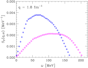
Figura 5.9: Nuclear matter response at $|{\bf q}|=1.8\ {\rm fm}^{-1}$. Diamonds and squares correspond to the FG model and the correlated HF approximation described in the text.

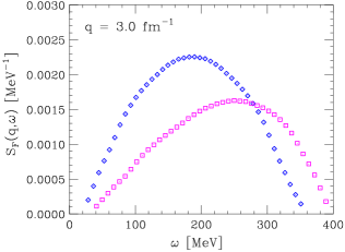
Figura 5.10: Same as in Fig. 5.9, for momentum transfer $|{\bf q}|=3.0\ {\rm fm}^{-1}$.

5.5 Tamm-Dancoff Approximation

In the previous section we have discussed the nuclear response in the correlated HF approximation, in which the bare Fermi transition operator is replaced by the effective operator of Eq.(5.14) and the final state is assumed to be a one particle-one hole state.

It is important to realize that the FG one particle-one hole states, while being eigenstates of the HF hamiltonian, defined as

$$H_{HF}=\sum_{i}e_{i}\ ,$$ (5.65)

with $e_{i}$ given by Eq.(2.63), are not eigenstates of the full nuclear hamiltonian. As a consequence, there is a residual interaction $V_{res}$ that can induce transitions between different one particle-one hole states, as long as their total momentum q, spin and isospin are conserved.

In order to include the effects of these transitions, we use the TD approximation, which amounts to expanding the final state in the basis of one particle-one hole states according to [106]

$$|f\rangle=|{\bf q},\ TSM\rangle=\sum_{i}c^{TSM}_{i}|{\bf h}_{i},\ {\bf p}_{i}={\bf h}_{i}+{\bf q},\ TSM\rangle\ ,$$ (5.66)

where $S$ and $T$ denote the total spin and isospin of the particle hole pair and $M$ is the spin projection.

At fixed ${\bf q}$, the excitation energy of the state (5.66), $\omega^{f}$, is obtained solving the eigenvalue equation

$$H|f\rangle=(E_{0}+\omega^{f})|f\rangle\ ,$$ (5.67)

where $E_{0}$ is the ground state energy. Substituting Eq.(5.66) into Eq.(5.67) and multiplying by $\langle{\bf h}_{j},\ {\bf p}_{j},\ TSM|$ from the left leads to

$$\sum_{i}\langle{\bf h}_{j},\ {\bf p}_{j},\ TSM|H|{\bf h}_{i},\ {\bf p}_{i},\ TSM\rangle\ c^{TSM}_{i} = \sum_{i}H^{TSM}_{ji}\ c^{TSM}_{i}$$ (5.68)

$$= (E_{0}+\omega^{TSM})c^{TSM}_{j}\ ,$$

with

$$H^{TSM}_{ji}=(E_{0}+e_{p_{i}}-e_{h_{i}})\delta_{ji}+\langle{\bf h}_{j},\ {\bf p}_{j},\ TSM|V_{res}|{\bf h}_{i},\ {\bf p}_{i},\ TSM_{S}\rangle\ ,$$ (5.69)

and [46]

$$\langle{\bf h}_{j},\ {\bf p}_{j},\ TSM|V_{res}|{\bf h}_{i},\ {\bf p}_{i},\ TSM\rangle=\langle v_{eff}\rangle_{D}-\langle v_{eff}\rangle_{E}\ .$$ (5.70)

In the above equation, $v_{eff}$ is the CFB effective interaction discussed in Chapter 2, and the direct and exchange contributions to the matrix elements are given by

$$\langle v_{eff}\rangle_{D}=\frac{1}{V^{2}}\int d^{3}r_{1}d^{3}r_{2}\ {\rm e}^{-i({\bf p}_{j}{\bf r}_{1}+{\bf h}_{i}{\bf r}_{2})}\ \langle\alpha_{p_{j}}\alpha_{h_{i}}|v_{eff}|\alpha_{h_{j}}\alpha_{p_{i}}\rangle\ {\rm e}^{i({\bf h}_{j}{\bf r}_{1}+{\bf p}_{i}{\bf r}_{2})}\ ,$$ (5.71)

$$\langle v_{eff}\rangle_{E}=\frac{1}{V^{2}}\int d^{3}r_{1}d^{3}r_{2}\ {\rm e}^{-i({\bf h}_{i}{\bf r}_{1}+{\bf p}_{j}{\bf r}_{2})}\ \langle\alpha_{h_{i}}\alpha_{p_{j}}|v_{eff}|\alpha_{h_{j}}\alpha_{p_{i}}\rangle\ {\rm e}^{i({\bf h}_{j}{\bf r}_{1}+{\bf p}_{i}{\bf r}_{2})}\ ,$$ (5.72)

where the two-nucleon state $|\alpha_{h}\alpha_{p}\rangle$ describes a hole in the spin-isospin state $\alpha_{h}$ and a particle in the spin-isospin state $\alpha_{p}$, coupled in such a way as to obtain the assigned values of $T$ and $S$ and $M$.

We can now exploit the fact that, in the case of Fermi transitions, the requirement that the matrix elements of $O^{F}_{eff}$ be non-vanishing implies that the particle hole pair be in a $S=1$ state with $M=\pm 1$. As a consequence, $H^{TSM}_{ij}$, $c^{TSM}_{i}$ and $\omega^{TSM}_{i}$ become independent of $M$.

For any fixed $T$ and $S$, the diagonalization of the hamiltonian matrix defined in Eqs.(5.69)-(5.72) determines the eigenvalues $\omega^{TS}_{n}$ and the the corresponding eigenvectors $c^{TS}_{n}$ with $n=1,\ 2,\ \ldots,\ N_{B}$, $N_{B}$ being the number of states in the one particle-one hole basis.

Collecting all the above results, we can finally write the response in the TD approximation as

$$S({\bf q},\omega)=\frac{1}{2}\sum_{T=0,1}\sum_{M=\pm 1}\ \sum_{n}\left|\sum_{i}(c^{T1}_{n})_{i}\langle{\bf h}_{i},\ {\bf p}_{i},\ T1M|O_{eff}({\bf q})|0\rangle\right|^{2}\delta(\omega-\omega^{T1}_{n})\ ,$$ (5.73)

where $(c^{T1}_{n})_{i}$ denotes the $i$-th component of the eigenvector belonging to the eigenvalue $\omega^{T1}_{n}$.

The main features of the response in the TD approximation can be understood considering a simple model in which $v_{eff}$ is assumed to be central and spin-isospin independent, and the exchange contribution to Eq.(5.70) is neglected. As a result we can make the replacement

$$\langle{\bf h}_{j},\ {\bf p}_{j},\ TSM|V_{res}|{\bf h}_{i},\ {\bf p}_{i},\ TSM\rangle\rightarrow\frac{2}{L^{3}}\int d^{3}r\ v_{eff}(r)\ {\rm e}^{i{\bf q}{\bf r}}\ =\hat{v}_{eff}(q)\ ,$$ (5.74)

leading to the eigenvalue equation

$$1=\hat{v}_{eff}(q)\sum_{i}\frac{1}{\omega-e_{p_{i}}+e_{h_{i}}}=\mathcal{F}(\omega)\ .$$ (5.75)

The above equation can be solved graphically plotting the right hand side as a function of $\omega$ and finding the intersections with the line $\mathcal{F}(\omega)=1$, as shown in Fig. 5.11 for $|{\bf q}|=0.3\ {\rm fm}^{-1}$ and a basis consisting of 8 states. The upper and lower panel correspond to $\hat{v}_{eff}(q)=-.06$ and 0.7 MeV, respectively. It appears that in the latter case the spectrum exhibits an eigenvalue lying well outside the particle hole continuum, corresponding to a collective excitation, reminiscent to the plasmon mode of the electron gas.

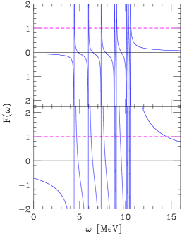
Figura 5.11: Graphical solution of Eq.(5.75) for $|{\bf q}|=0.3\ {\rm fm}^{-1}$ and a basis consisting of 8 states. The upper and lower panel correspond to $\hat{v}_{eff}(q)=-0.06$ and $-0.7$ MeV, respectively.

The nuclear matter response at $|{\bf q}|=0.3\ {\rm fm}^{-1}$ obtained using the TD approximation is shown in Fig. 5.12. The solid line in the lower left panel corresponds to the full calculation, including both the direct and exchange contributions to the matrix elements of the effective interactions (see Eq.(5.70)), while the solid line in the upper left panel has been obtained neglecting the exchange part. In both left panels, the dashed line refers to the correlated HF approximation. All calculation have been carried out using $\sim$ 3000 basis states.

The full TD response exhibits a sharp isolated peak corresponding to the collective mode, lying $\sim$ 4 MeV above the upper limit of the particle hole continuum. If only direct contributions are included, the peak is still clearly visible, but located at lower $\omega$, and not well separated from the continuum.

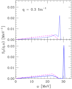
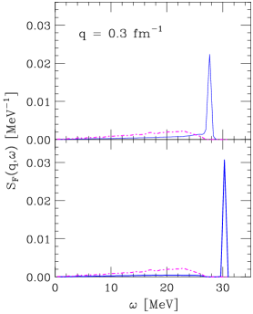
Figura 5.12: Nuclear matter response in the TD approximation at $|{\bf q}|=0.3\ {\rm fm}^{-1}$. The solid line in the upper left panel corresponds to the full calculation, while that in the lower left panel has been obtained neglecting the exchange term in Eq.(5.70). The dashed lines show the results of the correlated HF approximation. The right panels illustrate the contributions of the $T=0$ (solid lines) and $T=1$ (dash-dot lines) to the TD response, evaluated including direct and exchange terms (lower right) or direct term only (upper right).

The right panels of Fig. 5.12 illustrate the contributions to the TD response associated with different final states, corresponding to total isospin of the particle hole pair $T=0$ (solid lines) and $T=1$ (dashed lines). In the case of Fermi transitions, the total spin is $S=1$ and the two allowed spin projections, $M=\pm 1$ give equal contributions. The right lower and upper panels show the results of the full calculations and those obtained neglecting the exchange terms.

It clearly appears that the excitation of the collective mode is due to the antisymmetric $T=0$ state, while the strength arising from the symmetric $T=1$ state lies within the particle hole continuum.

Our correlated Hartree Fock results are in good agreement with those obtained by Cowell and Pandharipande using correlated states and a cluster expansion truncated at the two body level [31]. On the other hand, the results of Ref. [31] suggest that the inclusion of the exchange term of Eq.(5.70) is essential for the excitation of the coherent state, while our results show that the corresponding peak survives if exchange contributions are neglected. This discrepancy is likely to be ascribed to differences in the effective interactions.

Summary & Outlook

We have carried out calculations of the charged current weak response of nuclei and nuclear matter in both the low momentum transfer and the impulse approximation regimes. The quantitative understanding of this quantity is required in many areas of physics, ranging from simulations of supernov$\ae$ explosions and neutron star cooling to the analysis of neutrino oscillation experiments.

The calculation has been performed using a many-body approach based on a realistic nuclear hamiltonian, including two- and three-nucleon interactions, yielding a good description of the properties of both the two-nucleon systems and uniform nuclear matter.

At beam energies around 1 GeV, the formalism based on the target spectral function has been tested comparing the calculated cross sections to electron scattering data in the kinematical region corresponding to quasielastic scattering and $\Delta$-production, relevant to many long baseline oscillation experiments. The results suggest that, while the quasi elastic cross section is understood at the level of $\sim$ 10 %, the accurate description of the resonance region will require the extension of the available fits of the nucleon structure functions down to $Q^{2}\mathrel{\hbox to0.0pt{\lower 4.0pt\hbox{\hskip 1.0pt$\sim$}\hss}\raise 1.0pt\hbox{$<$}}$ 0.4 GeV², as proposed in Ref. [103].

In the high energy domain the differences between our results and the prediction of the FG model, widely used in the analysis of experimental data, mostly arise from the effects of short range nucleon-nucleon correlation. On the other hand, the response at low $|{\bf q}|$ (of the order of tens of MeV) is known to be sizably affected by long range correlations, giving rise to the excitation of collective modes.

The response associated with Fermi transitions at low momentum transfer has been calculated from an effective interaction, derived using the formalism of correlated basis functions and the cluster expansion technique. Our work improves upon existing effective interaction models in that it includes the effects of many-nucleon forces, which become sizable, at high density.

The energy per nucleon of both symmetric nuclear matter and pure neutron matter, obtained from our effective interaction model, turns out to be in fairly good agreement with the results of highly refined many body calculations, based on similar dynamical models. A comparable agreement with the results available in the literature has also been found for single particle properties, e.g. the effective mass, and the spin susceptibility. The emerging picture suggests that our approach can be regarded as an effective theory that captures the relevant physics, allowing one to obtain reasonable estimates of a number of different quantities using low order perturbation theory in the Fermi gas basis.

The responses calculated within the correlated HF approximation show that the inclusion of short range correlations leads to a significant quenching of the transition matrix elements and shifts the strength towards larger values of the energy transfer, $\omega$, for all values of $|{\bf q}|$. At low momentum transfer, long range correlations have been taken into account within the TD approximation. The excitation of the coherent state can be clearly seen in our results at $|{\bf q}|=0.3\ {\rm fm}^{-1}$.

The most straightforward extension of our approach is the calculation of the Gamow Teller response. The inclusion of finite temperature effects, needed to extract the observables relevant to supernov$\ae$ and proto-neutron star physics, also appears to be doable, in the low temperature region $T\ll m_{\pi}$.

As a final remark, it has to be pointed out that, while our approach can and should be further developed, the possible improvements only pertain the structure of the effective interaction and the inclusion of perturbative corrections, and do not involve going to higher order in the cluster expansion.

Although the contribution of clusters involving more than two nucleons is known to be, in general, non negligible, effective theories are in fact designed to provide lowest order results reasonably accounting for the available data.

In this context, however, the rationale underlying the choice of the two-nucleon cluster approximation, employed in our work, deserves a comment.

While being likely to be reasonable for use in nuclear matter limit, our procedure does not preserve the normalization of the many-body wave function. We plan to investigate quantitavely this issue using alternative truncation schemes, designed to guarantee the correct normalization at finite order in the cluster expansion [108, 109].

The most obvious improvement is the inclusion in $v_{\rm eff}$ of the non static components of NN potential, which are known to be needed to reproduce scattering data.

On the other hand, inclusion of higher order terms in the perturbative expansion, which is expected to be rapidly convergent, is necessary to take into account more complex mechanisms, that play a role in determining several properties of many-body systems as, for example, the effective mass at the Fermi surface [56].

Appendice A Properties of the operators $O^{n}_{ij}$

In this Appendix, we discuss the properties of the six operators defined in Eq.(1.16), as well as some useful properties of the Pauli matrices.

A.1 Pauli matrices

In the standard representation, in which $\sigma^{3}$ is chosen to be diagonal, the threee Pauli matrices are given by (we specialize here to the spin matrices $\sigma^{i}$: analog properties obviously hold for the isospin matrices $\tau^{i}$)

$$\sigma^{1}=\left(\begin{array}[]{rr}0&\phantom{-}1\\ 1&0\end{array}\right)\ \ ,\ \ \sigma^{2}=\left(\begin{array}[]{rr}0&-i\\ i&0\end{array}\right)\ \ ,\ \ \sigma^{3}=\left(\begin{array}[]{rr}1&0\\ 0&-1\end{array}\right)\ .$$ (A.1)

The Pauli matrices satisfy

$$\sigma^{i}\sigma^{j} = \delta_{ij}+i\epsilon_{ijk}\sigma^{k}\ ,$$ (A.2)

$$\epsilon_{ijk}\sigma^{j}\sigma^{k} = 2i\sigma^{i}\ ,$$ (A.3)

that can be put in the form

$$[\sigma^{i},\,\sigma^{j}] = 2i\epsilon_{ijk}\sigma^{k}\ ,$$ (A.4)

$$\{\sigma^{i},\,\sigma^{j}\} = 2\delta_{ij}\ ,$$ (A.5)

where $\epsilon_{ijk}$ is the totally antisymmetric tensor and $i,j,k=1,2,3$. The first properties shows that the Pauli matrices are the generators of an $SU(2)$ algebra.

A.2 Projection operators

Let now ${\bm{\sigma}}_{1}$ and ${\bm{\sigma}}_{2}$ be the vectors of Pauli matrices for particle 1 and 2, respectively (i.e. ${\bm{\sigma}}_{1}\equiv\left\{\sigma_{1}^{1},\,\sigma_{1}^{2},\,\sigma_{1}^{3}\right\}$). From the properties (A.2)-(A.3), it follows that

$$({\bm{\sigma}}_{1}\cdot{\bm{\sigma}}_{2})^{2}=3-2({\bm{\sigma}}_{1}\cdot{\bm{\sigma}}_{2})\ .$$ (A.6)

As $({\bm{\sigma}}_{1}\cdot{\bm{\sigma}}_{2})$ is a scalar quantity, we can interpret the above equation as an algebraic one, with solutions $({\bm{\sigma}}_{1}\cdot{\bm{\sigma}}_{2})=-3$ and $({\bm{\sigma}}_{1}\cdot{\bm{\sigma}}_{2})=1$. They correspond to the states of total spin $S=0$ (spin singlet channel) and $S=1$ (spin triplet channel), respectively. It is thus useful introducing the operators $P_{2S+1}$ (and the analog $\Pi_{2T+1}$ for the isospin states), defined as

$$P_{(S=0)}\equiv P_{1} = \frac{1-({\bm{\sigma}}_{1}\cdot{\bm{\sigma}}_{2})}{4}\ ,$$ (A.7)

$$P_{(S=1)}\equiv P_{3} = \frac{3+({\bm{\sigma}}_{1}\cdot{\bm{\sigma}}_{2})}{4}\ ,$$ (A.8)

which project onto states of definte total spin 0 or 1, respectively:

$$P_{2S+1}|S^{\prime}\rangle=\delta_{SS^{\prime}}|S^{\prime}\rangle\ ,$$ (A.9)

The projection operators satisfy to

$$P^{2}_{2S+1} = P^{\phantom{2}}_{2S+1}\ ,$$ (A.10)

$$P_{1}+P_{3} = \leavevmode\hbox{\small 1\kern-3.8pt\normalsize 1}\ ,$$ (A.11)

$$P_{1}P_{3}=P_{3}P_{1} = 0\ ,$$ (A.12)

where 11 is the two-dimensional identity matrix.

A.3 Spin and isospin exchange operators

Consider the two-nucleon spin states (or the analog isospin states)

$$|0\,0\rangle = \frac{1}{\sqrt{2}}\left(|\uparrow\downarrow\rangle-|\downarrow\uparrow\right)\ ,$$

$$|1-1\rangle = |\downarrow\downarrow\rangle\ ,$$

$$|1\,0\rangle = \frac{1}{\sqrt{2}}\left(|\uparrow\downarrow\rangle+|\downarrow\uparrow\right)\ ,$$

$$|1\,1\rangle = |\uparrow\uparrow\rangle\ ,$$

where $|0\,0\rangle\equiv|S=0\,M_{S}=0\rangle$ etc., and the inverse relations

$$|\uparrow\uparrow\rangle = |1\,1\rangle\ ,$$

$$|\uparrow\downarrow\rangle = \frac{1}{\sqrt{2}}\left(|1\,0\rangle+|0\,0\rangle\right)\ ,$$

$$|\downarrow\uparrow\rangle = \frac{1}{\sqrt{2}}\left(|1\,0\rangle-|0\,0\rangle\right)\ ,$$

$$|\downarrow\downarrow\rangle = |1\,-1\rangle\ .$$

From properties (A.9), and from

$$\left(P_{3}-P_{1}\right)|\uparrow\uparrow\rangle=|\uparrow\uparrow\rangle \left(P_{3}-P_{1}\right)|\downarrow\downarrow\rangle=|\downarrow\downarrow\rangle\ ,$$ ,

$$\left(P_{3}-P_{1}\right)|\uparrow\downarrow\rangle=|\downarrow\uparrow\rangle \left(P_{3}-P_{1}\right)|\downarrow\uparrow\rangle=|\uparrow\downarrow\rangle\ ,$$ ,

it follows that $P_{\sigma}\equiv P_{3}-P_{1}$ is the spin-exchange operator, satisfying

$$P_{\sigma}|S\,M_{S}\rangle=(-)^{S+1}|S\,M_{S}\rangle\ .$$ (A.13)

A similar exchange operator can be defined for isospin, $P_{\tau}\equiv\Pi_{3}-\Pi_{1}$, with

$$P_{\tau}|T\,M_{T}\rangle=(-)^{T+1}|T\,M_{T}\rangle\ .$$ (A.14)

Combining the above results we find

$$P_{\sigma\tau}\equiv P_{\sigma}P_{\tau}=\frac{1}{4}\,\Big{(}1+({\bm{\sigma}}_{1}\cdot{\bm{\sigma}}_{2})\Big{)}\Big{(}1+({\bm{\tau}}_{1}\cdot{\bm{\tau}}_{2})\Big{)}\ ,$$ (A.15)

with

$$P_{\sigma\tau}|S\,M_{S},\,T\,M_{T}\rangle=(-)^{S+T}|S\,M_{S},\,T\,M_{T}\rangle\ .$$ (A.16)

A.4 The tensor operator $S_{12}$

The tensor operator $S_{12}$ is defined as

$$S_{12}\equiv\frac{3}{r^{2}}\;\left({\bm{\sigma}}_{1}\cdot{\bf r}\right)\,\left({\bm{\sigma}}_{2}\cdot{\bf r}\right)-({\bm{\sigma}}_{1}\cdot{\bm{\sigma}}_{2})\ ,$$ (A.17)

where ${\bf r}$ is the relative coordinate of particels 1 and 2 while $r=|{\bf r}|$.

Making use of Eq.(A.2), it can be shown that

$$S_{12}({\bm{\sigma}}_{1}\cdot{\bm{\sigma}}_{2})=({\bm{\sigma}}_{1}\cdot{\bm{\sigma}}_{2})S_{12}=S_{12}\ .$$ (A.18)

As we saw, $({\bm{\sigma}}_{1}\cdot{\bm{\sigma}}_{2})=$ 1 on triplet states, while $({\bm{\sigma}}_{1}\cdot{\bm{\sigma}}_{2})=$ $-3$ on singlet states. The above equation thus implies that the tensor operator only acts on triplet states and

$$\left[S_{12},\;P_{3}\right]=0\ .$$ (A.19)

Moreover,

$$S^{2}_{12}=6-2S^{\phantom{2}}_{12}+2({\bm{\sigma}}_{1}\cdot{\bm{\sigma}}_{2})\ .$$ (A.20)

The tensor operator is a function of ${\bf r}$ satisfying

$${\bm{\nabla}}S_{12} = \frac{3}{r^{2}}\Bigg{[}{\bm{\sigma}}_{1}\left({\bm{\sigma}}_{2}\cdot{\bf r}\right)+{\bm{\sigma}}_{2}\left({\bm{\sigma}}_{1}\cdot{\bf r}\right)-2\frac{{\bf r}}{r^{2}}\left({\bm{\sigma}}_{1}\cdot{\bf r}\right)\,\left({\bm{\sigma}}_{2}\cdot{\bf r}\right)\Bigg{]}\ ,$$ (A.21)

$$\nabla^{2}S_{12} = -\frac{6}{r^{2}}S_{12}\ .$$ (A.22)

For any function $u(r)$, Eq.(A.21) implies

$$\left({\bm{\nabla}}u\right)\cdot\left({\bm{\nabla}}S_{12}\right)=\frac{du}{dr}\;\frac{{\bf r}}{r}\cdot\left({\bm{\nabla}}S_{12}\right)=0\ .$$ (A.23)

Moreover

$$\left({\bm{\nabla}}S_{12}\right)^{2} = \frac{6}{r^{2}}\left(8-S_{12}\right)\ ,$$ (A.24)

$$\left[S_{12},\;\left({\bm{\nabla}}S_{12}\right)\right] = \frac{36}{r^{2}}\;i\,\left({\bf S}\times{\bf r}\right)\ ,$$ (A.25)

$$\left[S_{12},\;\left({\bm{\nabla}}S_{12}\right)\right]{\bm{\nabla}} = \frac{36}{r^{2}}\;\left({\bf L}\cdot{\bf S}\right)\ ,$$ (A.26)

where ${\bf S}=\left({\bm{\sigma}}_{1}+{\bm{\sigma}}_{2}\right)/2$ and ${\bf L}={\bf r}\times{\bf p}=-i\left({\bf r}\times{\bm{\nabla}}\right)$ is the orbital angular momentum operator of the relative motion.

From Equation (A.22), we can calculate

$$\left[S_{12},\;\nabla^{2}S_{12}\right]=0\ ,$$ (A.27)

and

$$\left({\bm{\nabla}}S_{12}\right)\;\left[S_{12},\;{\bm{\nabla}}\right]=-\left({\bm{\nabla}}S_{12}\right)^{2}\ .$$ (A.28)

A.5 Operator algebra

Equations (A.6), (A.18) and (A.20) show that the six operators

$$O^{1,\ldots,6}=1,\;({\bm{\tau}}_{1}\cdot{\bm{\tau}}_{2}),\;({\bm{\sigma}}_{1}\cdot{\bm{\sigma}}_{2}),\;({\bm{\sigma}}_{1}\cdot{\bm{\sigma}}_{2})({\bm{\tau}}_{1}\cdot{\bm{\tau}}_{2}),\;S_{12},\;S_{12}({\bm{\tau}}_{1}\cdot{\bm{\tau}}_{2})\ \ ,$$ (A.29)

close an algebra, i.e. they satisfy

$$O^{i}O^{j}=\sum_{k}K^{k}_{ij}O^{k}\ .$$ (A.30)

The coefficients $K^{k}_{ij}$ are easily obtained by calculating

$$O^{1}O^{i}=O^{i}O^{1}=O^{i}\Longrightarrow K^{k}_{1i}=K^{k}_{i1}=\delta^{k}_{i}\$$

$$O^{2}O^{2}=3O^{2}-2O^{2}\Longrightarrow K^{k}_{22}=3\delta^{k}_{1}-2\delta^{k}_{2}\ ,$$

$$O^{2}O^{3}=O^{3}O^{2}=O^{4}\Longrightarrow K^{k}_{23}=K^{k}_{32}=\delta^{k}_{4}\ ,$$

$$O^{2}O^{4}=3O^{3}-2O^{4}\Longrightarrow K^{k}_{24}=K^{k}_{42}=\delta^{k}_{3}-1\delta^{k}_{4}\ ,$$

$$O^{2}O^{5}=O^{5}O^{2}=O^{6}\Longrightarrow K^{k}_{25}=K^{k}_{52}=\delta^{k}_{6}\ ,$$

$$O^{2}O^{6}=O^{6}O^{2}=3O^{5}-2O^{6}\Longrightarrow K^{k}_{26}=K^{k}_{62}=3\delta^{k}_{5}-2\delta^{k}_{6}\ ,$$

$$O^{3}O^{3}=3O^{1}-2O^{3}\Longrightarrow K^{k}_{33}=3\delta^{k}_{1}-2\delta^{k}_{3}\ ,$$

$$O^{3}O^{4}=O^{4}O^{3}=3O^{2}-2O^{4}\Longrightarrow K^{k}_{34}=K^{k}_{43}=3\delta^{k}_{2}-2\delta^{k}_{4}\ ,$$

$$O^{3}O^{5}=O^{5}O^{3}=O^{5}\Longrightarrow K^{k}_{35}=K^{k}_{53}=\delta^{k}_{5}\ ,$$

$$O^{3}O^{6}=O^{6}O^{3}=O^{6}\Longrightarrow K^{k}_{36}=K^{k}_{63}=\delta^{k}_{6}\ ,$$

$$O^{4}O^{4}=9O^{1}-6O^{2}-6O^{3}+4O^{4}\Longrightarrow K^{k}_{44}=9\delta^{k}_{1}-6\delta^{k}_{2}-6\delta^{k}_{3}+4\delta^{k}_{4}\ ,$$

$$O^{4}O^{5}=O^{5}O^{4}=O^{6}\Longrightarrow K^{k}_{45}=K^{k}_{54}=\delta^{k}_{6}\ ,$$

$$O^{4}O^{6}=O^{6}O^{4}=3O^{5}-2O^{6}\Longrightarrow K^{k}_{46}=K^{k}_{64}=3\delta^{k}_{5}-2\delta^{k}_{6}\ ,$$

$$O^{5}O^{5}=6O^{1}+2O^{3}-2O^{5}\Longrightarrow K^{k}_{55}=6\delta^{k}_{1}+2\delta^{k}_{3}-2\delta^{k}_{5}\ ,$$

$$O^{5}O^{6}=O^{6}O^{5}=6O^{2}+2O^{4}-2O^{6}\Longrightarrow K^{k}_{56}=K^{k}_{65}=6\delta^{k}_{2}+2\delta^{k}_{4}-2\delta^{k}_{6}\ ,$$

$$O^{6}O^{6} = 18O^{1}-12O^{2}+6O^{3}-4O^{4}-6O^{6}+4O^{6}$$

$$\ \ \ \ \ \ \ \ \ \ \ \ \ \ \ \ \Longrightarrow K^{k}_{66}=18\delta^{k}_{1}-12\delta^{k}_{2}+6\delta^{k}_{3}-4\delta^{k}_{4}-6\delta^{k}_{4}+4\delta^{k}_{6}\ .$$

A.6 Matrix elements

Finally, we report a number of expectation values of operators involving Pauli matrices, in two-nucleon states of definite total spin and isospion, $|S\;M_{S},\;T\;M_{T}\rangle$.

$$\langle P_{2S^{\prime}+1}\Pi_{2T^{\prime}+1}\rangle = \delta_{SS^{\prime}}\delta_{TT^{\prime}}\ ,$$ (A.31)

$$\langle P_{2S^{\prime}+1}\Pi_{2T^{\prime}+1}P_{\sigma\tau}\rangle = (-)^{S+T}\delta_{SS^{\prime}}\delta_{TT^{\prime}}\ ,$$ (A.32)

$$\sum_{SM_{S}}\delta_{S^{\prime}1}\langle S_{12}P_{2S^{\prime}+1}\Pi_{2T^{\prime}+1}\rangle = \delta_{S^{\prime}1}\delta_{TT^{\prime}}\sum_{M_{S}}\langle 1\;M_{S}|S_{12}|1\;M_{S}\rangle=0\ ,$$ (A.33)

$$\sum_{SM_{S}}\delta_{S^{\prime}1}\langle S_{12}P_{2S^{\prime}+1}\Pi_{2T^{\prime}+1}P_{\sigma\tau}\rangle = 0\ .$$ (A.34)

A.7 More matrix elements

The explicit expressions for the matrices entering Eq.(2.60), defined by

$$A^{i}_{\lambda\mu}=\langle\lambda\mu|O^{i}_{12}|\lambda\mu\rangle\ \ ,\ \ B^{i}_{\lambda\mu}=\langle\lambda\mu|O^{i}_{12}|\mu\lambda\rangle\ ,$$ (A.35)

where $|\lambda\mu\rangle$ denotes the two-nucleon spin-isospin state, can be easily obtained from the above properties of the six operators $O^{n\leq 6}$.

We find

$$A^{1} = \left(\begin{array}[]{llll}\phantom{-}1&\phantom{-}1&\phantom{-}1&\phantom{-}1\\ \phantom{-}1&\phantom{-}1&\phantom{-}1&\phantom{-}1\\ \phantom{-}1&\phantom{-}1&\phantom{-}1&\phantom{-}1\\ \phantom{-}1&\phantom{-}1&\phantom{-}1&\phantom{-}1\end{array}\right)\ ,$$ (A.40)

$$A^{2} = \left(\begin{array}[]{rrrr}1&1&-1&-1\\ 1&1&-1&-1\\ -1&-1&1&1\\ -1&-1&1&1\end{array}\right)\ ,$$ (A.45)

$$A^{3} = \left(\begin{array}[]{rrrr}1&-1&1&-1\\ -1&1&-1&1\\ 1&-1&1&-1\\ -1&1&-1&1\end{array}\right)\ ,$$ (A.50)

$$A^{4} = \left(\begin{array}[]{rrrr}1&-1&-1&1\\ -1&1&1&-1\\ -1&1&1&-1\\ 1&-1&-1&1\end{array}\right)\ ,$$ (A.55)

$$A^{5} = \left(\begin{array}[]{rrrr}1&1&-1&-1\\ 1&1&-1&-1\\ -1&-1&1&1\\ -1&-1&1&1\end{array}\right)\left(3\cos^{2}{\theta}-1\right)=A^{2}\left(3\cos^{2}{\theta}-1\right)\ ,$$ (A.60)

$$A^{6} = \left(\begin{array}[]{rrrr}1&-1&-1&1\\ -1&1&1&-1\\ -1&1&1&-1\\ 1&-1&-1&1\end{array}\right)\left(3\cos^{2}{\theta}-1\right)=A^{4}\left(3\cos^{2}{\theta}-1\right)\ ,$$ (A.65)

$$B^{1} = \left(\begin{array}[]{rrrr}\phantom{-}1&\phantom{-}0&\phantom{-}0&\phantom{-}0\\ \phantom{-}0&\phantom{-}1&\phantom{-}0&\phantom{-}0\\ \phantom{-}0&\phantom{-}0&\phantom{-}1&\phantom{-}0\\ \phantom{-}0&\phantom{-}0&\phantom{-}0&\phantom{-}1\end{array}\right)\ ,$$ (A.70)

$$B^{2} = \left(\begin{array}[]{rrrr}\phantom{-}1&\phantom{-}0&\phantom{-}2&\phantom{-}0\\ \phantom{-}0&\phantom{-}1&\phantom{-}0&\phantom{-}2\\ \phantom{-}2&\phantom{-}0&\phantom{-}1&\phantom{-}0\\ \phantom{-}0&\phantom{-}2&\phantom{-}0&\phantom{-}1\end{array}\right)\ ,$$ (A.75)

$$B^{3} = \left(\begin{array}[]{rrrr}\phantom{-}1&\phantom{-}2&\phantom{-}0&\phantom{-}0\\ \phantom{-}2&\phantom{-}1&\phantom{-}0&\phantom{-}0\\ \phantom{-}0&\phantom{-}0&\phantom{-}1&\phantom{-}2\\ \phantom{-}0&\phantom{-}0&\phantom{-}2&\phantom{-}1\end{array}\right)\ ,$$ (A.80)

$$B^{4} = \left(\begin{array}[]{rrrr}\phantom{-}1&\phantom{-}2&\phantom{-}2&\phantom{-}4\\ \phantom{-}2&\phantom{-}1&\phantom{-}4&\phantom{-}2\\ \phantom{-}2&\phantom{-}4&\phantom{-}1&\phantom{-}2\\ \phantom{-}4&\phantom{-}2&\phantom{-}2&\phantom{-}1\end{array}\right)\ ,$$ (A.85)

$$B^{5} = \left(\begin{array}[]{rrrr}1&-1&0&0\\ -1&1&0&0\\ 0&0&1&-1\\ 0&0&-1&1\end{array}\right)\,\left(3\cos^{2}{\theta}-1\right)\ ,$$ (A.90)

$$B^{6} = \left(\begin{array}[]{rrrr}1&-1&2&-2\\ -1&1&-2&2\\ 2&-2&1&-1\\ -2&2&-1&1\end{array}\right)\,\left(3\cos^{2}{\theta}-1\right)\ ,$$ (A.95)

where $\theta$ is the angle between ${\bf r}$ and the $z$ axis.

A.8 Change of representation

In this Section we discuss the different representation for the operators of the “$v_{6}$” algebra. A generic operator $x$ can be written as

$$x=\sum_{p=1}^{6}x^{p}_{ij}O^{p}=x_{c}+x_{\tau}({\bm{\tau}}_{1}\cdot{\bm{\tau}}_{2})+x_{\sigma}({\bm{\sigma}}_{1}\cdot{\bm{\sigma}}_{2})+x_{\sigma\tau}({\bm{\sigma}}_{1}\cdot{\bm{\sigma}}_{2})({\bm{\tau}}_{1}\cdot{\bm{\tau}}_{2})+x_{t}S_{12}+x_{t\tau}S_{12}({\bm{\tau}}_{1}\cdot{\bm{\tau}}_{2})\ ,$$ (A.96)

in the basis of operators (A.29), or as

$$x=\sum_{TS}\left[x_{T0}+\delta_{S1}x_{tT}S_{12}\right]P_{2S+1}\Pi_{2T+1}\ ,$$ (A.97)

in the “TS-representation”.

The transformation matrix is given by

$$\left(\begin{array}[]{rrrr}1&-3&-3&9\\ 1&1&-3&-3\\ 1&-3&1&-3\\ 1&1&1&1\end{array}\right)\left(\begin{array}[]{c}x_{c}\\ x_{\tau}\\ x_{\sigma}\\ x_{\sigma\tau}\end{array}\right)=\left(\begin{array}[]{c}x_{00}\\ x_{10}\\ x_{01}\\ x_{11}\end{array}\right)\ ,$$ (A.98)

$$\left(\begin{array}[]{rr}1&-3\\ 1&1\end{array}\right)\left(\begin{array}[]{c}x_{t}\\ x_{t\tau}\end{array}\right)=\left(\begin{array}[]{c}x_{t0}\\ x_{t1}\end{array}\right)\ ,$$ (A.99)

or

$$\left\{\begin{array}[]{l}x_{TS}=x_{c}+(4T-3)x_{\tau}+(4S-3)x_{\sigma}+(4S-3)(4T-3)x_{\sigma\tau}\ ,\\ \\ x_{tT}=x_{t}+(4T-3)x_{tT}\ .\end{array}\right.$$ (A.100)

The inverse transformation is given by

$$\frac{1}{16}\left(\begin{array}[]{rrrr}1&3&3&9\\ -1&1&-3&3\\ -1&-3&1&3\\ 1&-1&-1&1\end{array}\right)\left(\begin{array}[]{c}x_{00}\\ x_{10}\\ x_{01}\\ x_{11}\end{array}\right)=\left(\begin{array}[]{c}x_{c}\\ x_{\tau}\\ x_{\sigma}\\ x_{\sigma\tau}\end{array}\right)\ ,$$ (A.101)

$$\frac{1}{4}\left(\begin{array}[]{rr}1&3\\ -1&1\end{array}\right)\left(\begin{array}[]{c}x_{t0}\\ x_{t1}\end{array}\right)=\left(\begin{array}[]{c}x_{t}\\ x_{t\tau}\end{array}\right)\ ,$$ (A.102)

Appendice B Energy at two-body cluster level

The energy per particle at two-body cluster level can be written (see Eqs.(2.31) and (2.33))

$$(\Delta E)_{2}=\sum_{i<j}\>\langle ij|\>\frac{1}{2}\bigg{[}f_{12},\left[\;t_{1}+t_{2},\>f_{12}\right]\bigg{]}+f_{12}v_{12}f_{12}\>|ij-ji\rangle\ ,$$ (B.1)

with

$$t_{i}=-\frac{1}{2m}\nabla^{2}_{i}\ \ ,\ \ t_{1}+t_{2}=-\frac{1}{m}\nabla^{2}_{\phantom{R}}-\frac{1}{4m}\nabla^{2}_{R}\ ,$$ (B.2)

where ${\bm{\nabla}}$ acts on the relative coordinate ${\bf r}$, while ${\bm{\nabla}}_{R}$ acts on the center of mass coordinate ${\bf R}$, defined as

$${\bf r}={\bf r}_{1}-{\bf r}_{2}\ \ ,\ \ {\bf R}=\frac{1}{2}({\bf r}_{1}+{\bf r}_{2})$$ (B.3)

respectively.

Including only the static part of the interaction, i.e. neglecting the spin-orbit components, both the correlation function $f_{12}$ and the two-nucleon potential $v_{12}$ are written as

$$f_{12}=\sum^{6}_{p=1}f^{p}(r_{12})O^{p}_{12}\ \ ,\ \ v_{12}=\sum^{6}_{p=1}v^{p}(r_{12})O^{p}_{12}\ ,$$ (B.4)

with the six operator $O^{n}_{12}$ listed in Eq.(1.16), whose properties are discussed in Appendix A..

The FG two-nucleon state is given by

$$|ij\rangle = \frac{1}{V}\;{\rm e}^{i({\bf k}_{i}\cdot{\bf r}_{1}+{\bf k}_{j}\cdot{\bf r}_{2})}\;|S\,M_{S},\,T\,M_{T}\rangle$$ (B.5)

$$= \frac{1}{V}\;{\rm e}^{i({\bf k}\cdot{\bf r}+{\bf K}\cdot{\bf R})}\;|S\,M_{S},\,T\,M_{T}\rangle\ ,$$

where

$$|{\bf k}_{i}|,\;|{\bf k}_{j}| \leq p_{F}$$

$${\bf k}=\frac{1}{2}({\bf k}_{i}-{\bf k}_{j})\ \ {\bf K}={\bf k}_{i}+{\bf k}_{j}\ ,$$ , (B.6)

and $|S\,M_{S},\,T\,M_{T}\rangle$ denotes a state of total spin (isospin) $S\ (T)$ and spin (isospin) projection $M_{S}\ (M_{T})$.

We will discuss the potential and kinetic energy term separately.

B.1 Potential energy

Consider the operator

$$w_{12}=f_{12}v_{12}f_{12}\ ,$$ (B.7)

and the decomposition of $f_{12}$ in the $TS$-representation (see Eq.(A.97))

$$f_{12}=\sum_{ST}\bigg{[}f_{ST}+\delta_{S1}f_{tT}S_{12}\bigg{]}P^{\phantom{2}}_{2S+1}\Pi^{\phantom{2}}_{2T+1}\ .$$ (B.8)

In the above equation, $P^{\phantom{2}}_{2S+1}$ and $\Pi^{\phantom{2}}_{2T+1}$ are spin and isospin projection operators, whose properties are given in Appendix A. By writing the corresponding decomposition for $w_{12}$ and $v_{12}$ and calculating

$$w_{12} = \sum_{TS}\Bigg{\{}\delta^{\phantom{2}}_{S0}f^{2}_{T0}v^{\phantom{2}}_{T0}+\delta_{S1}\Big{\{}\;v^{\phantom{2}}_{T1}\bigg{[}\;f^{2}_{T1}+8f^{2}_{tT}+2\left(f^{\phantom{2}}_{T1}f^{\phantom{2}}_{tT}-f^{2}_{tT}\right)S_{12}\bigg{]}+$$

$$+ \!\!v^{\phantom{2}}_{tT}\bigg{[}16\left(f^{\phantom{2}}_{T1}f^{\phantom{2}}_{tT}-f^{2}_{tT}\right)+\left(f^{2}_{T1}-4f^{\phantom{2}}_{T1}f^{\phantom{2}}_{tT}+12f^{2}_{t1}\right)S_{12}\bigg{]}\Big{\}}\Bigg{\}}P^{\phantom{2}}_{2S+1}\Pi^{\phantom{2}}_{2T+1}\ ,$$

we can identify

$$w^{\phantom{2}}_{T0} = \phantom{2}v^{\phantom{2}}_{T0}\phantom{\Big{(}}f^{2}_{T0}\phantom{\Big{)}}$$

$$w^{\phantom{2}}_{T1} = \phantom{2}v^{\phantom{2}}_{T1}\Big{(}f^{2}_{T1}+8f^{2}_{tT}\Big{)}+16v^{\phantom{2}}_{tT}\Big{(}f^{\phantom{2}}_{T1}f^{\phantom{2}}_{tT}-f^{2}_{tT}\Big{)}$$ (B.9)

$$w^{\phantom{2}}_{tT} = 2v^{\phantom{2}}_{T1}\Big{(}f^{\phantom{2}}_{T1}f^{\phantom{2}}_{tT}-f^{2}_{tT}\Big{)}+v^{\phantom{2}}_{tT}\Big{(}f^{2}_{T1}-4f^{\phantom{2}}_{T1}f^{\phantom{2}}_{tT}+12f^{2}_{t1}\Big{)}\ .$$

After replacing

$$\sum_{i<j}\longrightarrow\frac{1}{2}\,\sum_{ij}\ ,$$ (B.10)

the potential energy contribution to $(\Delta E)_{2}$ reads

$$\langle w\rangle = \frac{1}{2}\frac{1}{V^{2}}\sum_{SM_{S}}\sum_{TM_{T}}\sum_{{\bf k}_{i}{\bf k}_{j}}\sum_{S^{\prime}T^{\prime}}\Bigg{\{}\int\!d^{3}r_{1}d^{3}r_{2}\bigg{[}w_{S^{\prime}T^{\prime}}(r)\langle P_{2S^{\prime}+1}\Pi_{2T^{\prime}+1}\rangle+$$

$$\delta_{S^{\prime}1}w_{tT^{\prime}}(r)\langle S_{12}P_{2S^{\prime}+1}\Pi_{2T^{\prime}+1}\rangle\bigg{]}-\int\!d^{3}r_{1}d^{3}r_{2}\,{\rm e}^{i({\bf k}_{i}\cdot{\bf r}-{\bf k}_{j}\cdot{\bf r})}$$

$$\bigg{[}w_{S^{\prime}T^{\prime}}(r)\langle P_{2S^{\prime}+1}\Pi_{2T^{\prime}+1}P_{\sigma\tau}\rangle+\delta_{S^{\prime}1}w_{tT^{\prime}}(r)\langle S_{12}P_{2S^{\prime}+1}\Pi_{2T^{\prime}+1}P_{\sigma\tau}\rangle\bigg{]}\Bigg{\}}\ ,$$

where $P_{\sigma\tau}$ is the spin-isospin exchange operator defined in Appendix A and the expectation values $\langle O\rangle$ are taken over two-nucleon states of definite total spin and isospin $|S\,M_{S},\,T\,M_{T}\rangle$. Using

$$\int d^{3}r_{1}d^{3}r_{2}=\int d^{3}r\,d^{3}R=V\int d^{3}r\ ,$$ (B.12)

the definition of the Slater function (2.61),

$$\sum_{|{\bf k}|\leq p_{F}}{\rm e}^{i{\bf k}\cdot{\bf r}}=\frac{V}{(2\pi)^{3}}\int_{|{\bf k}|\leq p_{F}}d^{3}k\,e^{i{\bf k}\cdot{\bf r}}=\frac{N}{\nu}\ell(p_{F}r)\ ,$$ (B.13)

and the results of Appendix A, we finally obtain

$$\langle w\rangle=\frac{1}{2}\frac{1}{V^{2}}\frac{N^{2}}{\nu^{2}}V\sum_{ST}\left(2S+1\right)\left(2T+1\right)\int d^{3}r\,w_{ST}(r)\left[1-(-1)^{S+T}\ell^{2}(p_{F}r)\right]\ ,$$ (B.14)

where $\nu$ denotes the degeneracy of the momentum eigenstates. In the case of symmetric nuclear matter ($\nu=4$)

$$\frac{1}{N}\langle w\rangle = \frac{\rho}{32}\int d^{3}r\Big{\{}\big{[}w_{00}(r)+9w_{11}(r)\big{]}a_{-}(p_{F}r)+$$ (B.15)

$$\phantom{\frac{\rho}{32}\int d^{3}r}\!\!+\big{[}3w_{01}(r)+3w_{10}(r)\big{]}a_{+}(p_{F}r)\big{]}\Big{\}}\ ,$$

where $\rho=N/V$ is the density and

$$a_{\pm}(x)=1\pm\ell^{2}(x)\ .$$ (B.16)

B.2 Kinetic energy

Let us now discuss the kinetic contribution to the energy, given by

$$\frac{1}{2}\bigg{[}f_{12},\left[\;t_{1}+t_{2},\>f_{12}\right]\bigg{]}=-\frac{1}{2m}\bigg{[}f_{12},\left[\;\nabla^{2},\>f_{12}\right]\bigg{]}\ .$$ (B.17)

We consider spin-zero and spin-one channels separately.

Spin-zero channels

In these channels, the relevant part of the correlation function is given by

$$f_{12}=\sum_{T}f_{T0}(r)\;P_{1}\Pi_{2T+1}\ .$$ (B.18)

Making use of the results of Appendix A, as well as of

$$\Big{[}f_{T0},\,\nabla^{2}f_{T0}\Big{]}=0\ \ ,\ \ \Big{[}f_{T0},\,\big{(}{\bm{\nabla}}f_{T0}\big{)}{\bm{\nabla}}\Big{]}=-\big{(}{\bm{\nabla}}f_{T0}\big{)}^{2}\ ,$$ (B.19)

we find

$$\Big{[}f_{12},\left[\;\nabla^{2},\>f_{12}\right]\Big{]} = \sum_{TT^{\prime}}\Big{[}f_{T0}\;P^{\phantom{2}}_{1}\Pi^{\phantom{2}}_{2T+1},\left[\nabla^{2},\;f_{T0}\right]\;P^{\phantom{2}}_{1}\Pi^{\phantom{2}}_{2T^{\prime}+1}\Big{]}$$ (B.20)

$$= \sum_{TT^{\prime}}\Big{[}f_{T0},\left[\nabla^{2},\;f_{T0}\right]\Big{]}\;P^{2}_{1}\Pi^{\phantom{2}}_{2T+1}\Pi^{\phantom{2}}_{2T^{\prime}+1}$$

$$= \sum_{T}\Big{[}f_{T0},\,\big{(}\nabla^{2}f_{T0}\big{)}+2\big{(}{\bm{\nabla}}f_{T0}\big{)}{\bm{\nabla}}\Big{]}\;P^{\phantom{2}}_{1}\Pi^{\phantom{2}}_{2T+1}$$

$$= 2\sum_{T}\Big{[}f_{T0},\,\big{(}{\bm{\nabla}}f_{T0}\big{)}{\bm{\nabla}}\Big{]}\;P^{\phantom{2}}_{1}\Pi^{\phantom{2}}_{2T+1}$$

$$= -2\sum_{T}\big{(}{\bm{\nabla}}f_{T0}\big{)}^{2}\;P^{\phantom{2}}_{1}\Pi^{\phantom{2}}_{2T+1}\ .$$

Finally,

$$-\frac{1}{2m}\bigg{[}f_{12},\left[\;\nabla^{2},\>f_{12}\right]\bigg{]}=\frac{1}{m}\sum_{T}\big{(}{\bm{\nabla}}f_{T0}\big{)}^{2}\;P^{\phantom{2}}_{1}\Pi^{\phantom{2}}_{2T+1}\ .$$ (B.21)

Spin-one channels

In these channels, the correlation function is given by

$$f_{12}=\sum_{T}\bigg{[}f_{T1}(r)+f_{tT}(r)S_{12}\bigg{]}P^{\phantom{2}}_{3}\Pi^{\phantom{2}}_{2T+1}\ .$$ (B.22)

Relying once more on Appendix A, we calculate

$$\sum_{T^{\prime}}\Big{[}\nabla^{2},\,\big{(}f_{T^{\prime}1}+f_{tT^{\prime}}S_{12}\big{)}P^{\phantom{2}}_{3}\Pi^{\phantom{2}}_{2T^{\prime}+1}\Big{]}=\sum_{T^{\prime}}\Big{\{}\big{[}\nabla^{2},\,f_{T^{\prime}1}\big{]}+\big{[}\nabla^{2},\,f_{tT^{\prime}}S_{12}\big{]}\Big{\}}P^{\phantom{2}}_{3}\Pi^{\phantom{2}}_{2T^{\prime}+1}$$

$$=\sum_{T^{\prime}}\Big{\{}\big{(}\nabla^{2}f_{T^{\prime}1}\big{)}+2\big{(}{\bm{\nabla}}f_{tT^{\prime}}\big{)}{\bm{\nabla}}+\big{(}\nabla^{2}f_{tT^{\prime}}S_{12}\big{)}+2\big{(}{\bm{\nabla}}f_{tT^{\prime}}S_{12}\big{)}{\bm{\nabla}}\Big{\}}P^{\phantom{2}}_{3}\Pi^{\phantom{2}}_{2T^{\prime}+1}$$

$$=\sum_{T^{\prime}}\Big{\{}\big{(}\nabla^{2}f_{T^{\prime}1}\big{)}+2\big{(}{\bm{\nabla}}f_{tT^{\prime}}\big{)}{\bm{\nabla}}+\big{(}\nabla^{2}f_{tT^{\prime}}\big{)}S_{12}+\big{(}\nabla^{2}S_{12}\big{)}f_{tT^{\prime}}$$

$$+2\big{(}{\bm{\nabla}}f_{tT^{\prime}}\big{)}\big{(}{\bm{\nabla}}S_{12}\big{)}+2S_{12}\big{(}{\bm{\nabla}}f_{tT^{\prime}}\big{)}{\bm{\nabla}}+2f_{tT^{\prime}}\big{(}{\bm{\nabla}}S_{12}\big{)}{\bm{\nabla}}\Big{\}}P^{\phantom{2}}_{3}\Pi^{\phantom{2}}_{2T^{\prime}+1}\ .$$ (B.23)

Hence, the commutator in Eq.(B.17) can be rewritten as

$$\Big{[}f_{12},\left[\;\nabla^{2},\>f_{12}\right]\Big{]} = \sum_{TT^{\prime}}\Big{[}\big{(}f_{T1}+f_{tT}S_{12}\big{)}P^{\phantom{2}}_{3}\Pi^{\phantom{2}}_{2T+1},\left\{\ldots\right\}P^{\phantom{2}}_{3}\Pi^{\phantom{2}}_{2T^{\prime}+1}\Big{]}$$ (B.24)

$$= \sum_{T}\Big{[}f_{T1}+f_{tT}S_{12},\left\{\ldots\right\}\Big{]}P^{\phantom{2}}_{3}\Pi^{\phantom{2}}_{2T+1}$$

$$= \sum_{T}\Big{(}F^{(1)}_{T}+F^{(2)}_{T}\Big{)}P^{\phantom{2}}_{3}\Pi^{\phantom{2}}_{2T+1}\ ,$$

with

$$F^{(1)}_{T}=\Big{[}f_{T1},\left\{\ldots\right\}\Big{]}\ \ ,\ \ F^{(2)}_{T}=\Big{[}f_{tT}S_{12},\left\{\ldots\right\}\Big{]}\ ,$$ (B.25)

and

$$\Big{\{}\ldots\Big{\}} = \Big{\{}\big{(}\nabla^{2}f_{T^{\prime}1}\big{)}+2\big{(}{\bm{\nabla}}f_{tT^{\prime}}\big{)}{\bm{\nabla}}+\big{(}\nabla^{2}f_{tT^{\prime}}\big{)}S_{12}+\big{(}\nabla^{2}S_{12}\big{)}f_{tT^{\prime}}$$ (B.26)

$$+ 2\big{(}{\bm{\nabla}}f_{tT^{\prime}}\big{)}\big{(}{\bm{\nabla}}S_{12}\big{)}+2S_{12}\big{(}{\bm{\nabla}}f_{tT^{\prime}}\big{)}{\bm{\nabla}}+2f_{tT^{\prime}}\big{(}{\bm{\nabla}}S_{12}\big{)}{\bm{\nabla}}\Big{\}}\ .$$

We find

$$F^{(1)}_{T}=-2\big{(}{\bm{\nabla}}f_{T1}\big{)}^{2}-2\big{(}{\bm{\nabla}}f_{T1}\big{)}\big{(}{\bm{\nabla}}f_{tT}\big{)}S_{12}\ ,$$ (B.27)

and

$$F^{(2)}_{T} = \Big{[}f_{tT}S_{12},\,2\big{(}{\bm{\nabla}}f_{T1}\big{)}{\bm{\nabla}}\Big{]}+\Big{[}f_{tT}S_{12},\,2S_{12}\big{(}{\bm{\nabla}}f_{T1}\big{)}{\bm{\nabla}}\Big{]}+$$ (B.28)

$$+\Big{[}f_{tT}S_{12},\,2f_{T1}\big{(}{\bm{\nabla}}S_{12}\big{)}{\bm{\nabla}}\Big{]}=$$

$$= -2\big{(}{\bm{\nabla}}f_{T1}\big{)}\big{(}{\bm{\nabla}}f_{tT}\big{)}S_{12}-2\big{(}{\bm{\nabla}}f_{tT}\big{)}^{2}S^{2}_{12}+$$

$$+2f^{2}_{tT}\Big{[}S_{12},\,\big{(}{\bm{\nabla}}S_{12}\big{)}{\bm{\nabla}}\Big{]}$$

$$= -2\phantom{\Bigg{[}}\big{(}{\bm{\nabla}}f_{T1}\big{)}\big{(}{\bm{\nabla}}f_{tT}\big{)}S_{12}-2\big{(}{\bm{\nabla}}f_{tT}\big{)}^{2}\big{(}8-2S_{12}\big{)}\phantom{\Bigg{]}}+$$

$$- 2f^{2}_{tT}\Bigg{[}\frac{36}{r^{2}}\;\big{(}{\bf L}\cdot{\bf S}\big{)}+\frac{6}{r^{2}}\;\big{(}8-S_{12}\big{)}\Bigg{]}\ .$$

Collecting all pieces togheter, we find for the spin-one channels

$$-\frac{1}{2m}\bigg{[}f_{12},\left[\;\nabla^{2},\>f_{12}\right]\bigg{]} = \frac{1}{m}\sum_{T}\Bigg{\{}\big{(}{\bm{\nabla}}f_{T1}\big{)}^{2}+\big{(}{\bm{\nabla}}f_{T1}\big{)}\big{(}{\bm{\nabla}}f_{tT}S_{12}\big{)}+$$ (B.29)

$$+\phantom{\Bigg{[}}\big{(}{\bm{\nabla}}f_{tT}\big{)}^{2}\big{(}8-2S_{12}\big{)}\phantom{\Bigg{]}}+f^{2}_{tT}\Bigg{[}\frac{36}{r^{2}}\;\big{(}{\bf L}\cdot{\bf S}\big{)}+\frac{6}{r^{2}}\;\big{(}8-S_{12}\big{)}\Bigg{]}\Bigg{\}}P^{\phantom{2}}_{3}\Pi^{\phantom{2}}_{2T+1}$$

$$= \frac{1}{m}\sum_{TS}\Bigg{\{}\big{(}{\bm{\nabla}}f_{TS}\big{)}^{2}+\delta_{S1}\Big{[}2\big{(}{\bm{\nabla}}f_{TS}\big{)}\big{(}{\bm{\nabla}}f_{tT}\big{)}S_{12}+$$

$$+\big{(}{\bm{\nabla}}f^{\phantom{2}}_{tT}\big{)}^{2}S^{2}_{12}+f^{\phantom{2}}_{tT}\frac{36}{r^{2}}\;\big{(}{\bf L}\cdot{\bf S}\big{)}+\frac{6}{r^{2}}\;\big{(}8-S_{12}\big{)}\Big{]}\Bigg{\}}P^{\phantom{2}}_{2S+1}\Pi^{\phantom{2}}_{2T+1}$$

$$= \sum_{TS}\Big{\{}t_{TS}(r)+\delta_{S1}\bigg{[}t_{tT}(r)S_{12}+t_{bT}(r)\big{(}{\bf L}\cdot{\bf S}\big{)}\bigg{]}\Big{\}}P^{\phantom{2}}_{2S+1}\Pi^{\phantom{2}}_{2T+1}\ ,$$

with

$$t_{T0} = \frac{1}{m}\big{(}{\bm{\nabla}}f_{T0}\big{)}^{2}$$

$$t_{T1} = \frac{1}{m}\Big{[}\big{(}{\bm{\nabla}}f_{T1}\big{)}^{2}+8\big{(}{\bm{\nabla}}f_{tT}\big{)}^{2}+\frac{48}{r^{2}}\;f^{2}_{tT}\Big{]}$$

$$t_{tT} = \frac{1}{m}\Big{[}2\big{(}{\bm{\nabla}}f_{T1}\big{)}\big{(}{\bm{\nabla}}f_{tT}\big{)}-2\big{(}{\bm{\nabla}}f_{tT}\big{)}^{2}-\frac{6}{r^{2}}\;f^{2}_{tT}\Big{]}$$

$$t_{bT} = \frac{1}{m}\frac{36}{r^{2}}\;f^{2}_{tT}\ .$$

B.3 Final expression

We can rewrite

$$\left(\Delta E\right)_{2}=\sum_{i<j}\langle ij|W_{12}|ij-ji\rangle\ ,$$ (B.30)

with

$$W_{12}=-\frac{1}{m}\bigg{[}f_{12},\left[\;\nabla^{2},\>f_{12}\right]\bigg{]}+f_{12}v_{12}f_{12}$$

$$=\sum_{TS}\Big{\{}W_{TS}(r)+\delta_{S1}\bigg{[}W_{tT}(r)S_{12}+W_{bT}(r)\big{(}{\bf L}\cdot{\bf S}\big{)}\bigg{]}\Big{\}}P^{\phantom{2}}_{2S+1}\Pi^{\phantom{2}}_{2T+1}\ ,$$

where

$$W_{T0} = \frac{1}{m}\big{(}{\bm{\nabla}}f^{\phantom{2}}_{T0}\big{)}^{2}+v_{T0}f^{2}_{T0}$$

$$W_{T1} = \frac{1}{m}\Big{[}\big{(}{\bm{\nabla}}f_{T1}\big{)}^{2}+8\big{(}{\bm{\nabla}}f_{tT}\big{)}^{2}+\frac{48}{r^{2}}\;f^{2}_{tT}\Big{]}+$$

$$+v^{\phantom{2}}_{T1}\Big{(}f^{2}_{T1}+8f^{2}_{tT}\Big{)}+16v^{\phantom{2}}_{tT}\Big{(}f^{\phantom{2}}_{T1}f^{\phantom{2}}_{tT}-f^{2}_{tT}\Big{)}$$

$$W_{tT} = \frac{1}{m}\Big{[}2\big{(}{\bm{\nabla}}f_{T1}\big{)}\big{(}{\bm{\nabla}}f_{tT}\big{)}-2\big{(}{\bm{\nabla}}f_{tT}\big{)}^{2}-\frac{6}{r^{2}}\;f^{2}_{tT}\Big{]}+$$

$$+2v^{\phantom{2}}_{T1}\Big{(}f^{\phantom{2}}_{T1}f^{\phantom{2}}_{tT}-f^{2}_{tT}\Big{)}+v^{\phantom{2}}_{tT}\Big{(}f^{2}_{T1}-4f^{\phantom{2}}_{T1}f^{\phantom{2}}_{tT}+12f^{2}_{t1}\Big{)}$$

$$W_{bT} = \frac{1}{m}\;\frac{36}{r^{2}}\;f^{2}_{tT}\ .$$

Making use of the expression for the expectation values given in Appendix A, we finally obtain (compare to Eq.(B.15))

$$\frac{(\Delta E)_{2}}{N} = \frac{\rho}{32}\int\;d^{3}r\Bigg{\{}\Big{[}W_{00}(r)+9W_{11}(r)\Big{]}a_{-}(p_{F}r)+$$ (B.31)

$$+\Big{[}3W_{01}(r)+3W_{10}(r)\Big{]}a_{+}(p_{F}r)\Bigg{\}}\ .$$

Appendice C Euler-Lagrange equations for the correlation functions

C.1 Spin singlet channels: uncoupled equations

In the spin-zero channels, the energy per partcicle of SNM, evaluated at two-body cluster level, reads (compare to Eqs.(B.15) and (B.21))

$$\frac{(\Delta E)_{2}}{N} = \frac{\rho}{32}\;\left(2T+1\right)\int\;d^{3}r\left[\frac{1}{m}\big{(}{\bm{\nabla}}f^{\phantom{2}}_{T0}\big{)}^{2}+v_{T0}f^{2}_{T0}\right]a_{T0}(p_{F}r)$$ (C.1)

$$= \frac{\rho}{32}\;\left(2T+1\right)\;4\pi\int\;r^{2}dr\left[\frac{1}{m}\big{(}f^{\prime}_{T0}\big{)}^{2}+v_{T0}f^{2}_{T0}\right]a_{T0}(p_{F}r)$$

$$= \textrm{const}\;\int^{\infty}_{0}dr\;F\left[f^{\phantom{{}^{\prime}}}_{T0},\;f^{\prime}_{T0}\right]\ ,$$

where $a_{TS}(x)=1-(-)^{T+S}\ell^{2}(x)$ and

$$F\left[f^{\phantom{{}^{\prime}}}_{T0},\;f^{\prime}_{T0}\right]=\Bigg{[}\big{(}f^{\prime}_{T0}\big{)}^{2}+m\;v_{T0}f^{2}_{T0}\Bigg{]}\phi^{2}_{T0}\ ,$$ (C.2)

with

$$\phi_{T0}=r\sqrt{a_{T0}}\ .$$ (C.3)

The corresponding Euler-Lagrange (EL) equations for the unknown functions $f_{T0}$ are given by

$$\frac{d}{dr}\frac{\partial F}{\partial f^{\prime}_{T0}}-\frac{\partial F}{\partial f^{\phantom{{}^{\prime}}}_{T0}}=0\ .$$ (C.4)

From

$$\frac{\partial F}{\partial f^{\phantom{{}^{\prime}}}_{T0}} = 2\;m\;v_{T0}\;f^{2}_{T0}\;\phi^{2}_{T0}\ ,$$

$$\frac{\partial F}{\partial f^{\prime}_{T0}} = 2\;f^{\prime}_{T0}\;\phi^{2}_{T0}\ ,$$

$$\frac{d}{dr}\frac{\partial F}{\partial f^{\prime}_{T0}} = 2\;f^{\prime\prime}_{T0}\;\phi^{2}_{T0}+4\;f^{\prime}_{T0}\;\phi^{\prime}_{T0}\;\phi_{T0}\ ,$$ (C.5)

we obtain

$$f^{\prime\prime}_{T0}\;\phi^{2}_{T0}+2\;f^{\prime}_{T0}\;\phi^{\prime}_{T0}-m\;v_{T0}\;f^{2}_{T0}\;\phi^{2}_{T0}=0\ .$$ (C.6)

Introducing

$$g_{T0}\equiv f_{T0}\;\phi_{T0}\ ,$$ (C.7)

we can put Eq.(C.6) in the form

$$g^{\prime\prime}_{T0}-\Bigg{(}\frac{\phi^{\prime\prime}_{T0}}{\phi_{T0}}+m\;v_{T0}\Bigg{)}\;g_{T0}=0\ .$$ (C.8)

Now we introduce a Lagrange multiplier, in order to fulfill the requirement (see Eqs.(2.56)-(2.58))

$$\left.g^{\prime}_{T0}\right|_{r=d}=\left.\phi^{\prime}_{T0}\right|_{r=d}\ .$$ (C.9)

The resulting equation is Eq.(4) of Ref.[107]

$$g^{\prime\prime}_{T0}-\Bigg{(}\frac{\phi^{\prime\prime}_{T0}}{\phi_{T0}}+m\;\left(v_{T0}+\lambda\right)\Bigg{)}\;g_{T0}=0\ ,$$ (C.10)

to be integrated with the boundary conditions

$$\left.g_{T0}\right|_{r=0} = 0\ \ ,$$ (C.11)

$$\left.g_{T0}\right|_{r=d} = \left.\phi_{T0}\right|_{r=d}\ .$$ (C.12)

C.2 Spin triplet channels: coupled equations

In the spin-one channels, the contribution to the energy is given by (see Eqs.(B.15) and (B.31))

$$\frac{(\Delta E)_{2}}{N} = \frac{\rho}{32}\;\left(2T+1\right)\int\;d^{3}r\Bigg{\{}\frac{1}{m}\left[\big{(}{\bm{\nabla}}f^{\phantom{2}}_{T1}\big{)}^{2}+8\big{(}{\bm{\nabla}}f^{\phantom{2}}_{tT}\big{)}^{2}+\frac{48}{r^{2}}\;f^{2}_{tT}\right]+$$ (C.13)

$$+v_{T1}\bigg{(}f^{2}_{T1}+8f^{2}_{tT}\bigg{)}+16v_{tT}\bigg{(}f^{\phantom{2}}_{T1}f^{\phantom{2}}_{tT}-f^{2}_{tT}\bigg{)}\Bigg{\}}\;a_{T1}(p_{F}r)$$

$$= \textrm{const}\;\int^{\infty}_{0}dr\;F\left[f^{\phantom{{}^{\prime}}}_{T1},\;f^{\phantom{{}^{\prime}}}_{tT};\;f^{\prime}_{T1},\;f^{\prime}_{tT}\right]\ ,$$

where

$$F\left[f^{\phantom{{}^{\prime}}}_{T1},\;f^{\phantom{{}^{\prime}}}_{tT};\;f^{\prime}_{T1},\;f^{\prime}_{tT}\right] = \left(f^{\prime}_{T1}\right)^{2}\phi^{2}_{T1}+8\left(f^{\prime}_{tT}\right)^{2}\phi^{2}_{T1}+\frac{48}{r^{2}}\;f^{2}_{tT}\phi^{2}_{T1}+\ \ \ \ \ \ \ \ \ \ \ \ \ \ \ \ \$$ (C.14)

$$+ m\Big{[}v_{T1}\left(f^{2}_{T1}+8f^{2}_{tT}\right)+16v_{tT}\left(f^{\phantom{2}}_{T1}f^{\phantom{2}}_{tT}-f^{2}_{tT}\right)\Big{]}\ .$$

In this case we have two coupled EL equations

$$\left\{\begin{array}[]{l}\frac{d}{dr}\frac{\partial F}{\partial f^{\prime}_{T1}}-\frac{\partial F}{\partial f^{\phantom{{}^{\prime}}}_{T1}}=0\\ \\ \frac{d}{dr}\frac{\partial F}{\partial f^{\prime}_{tT}}-\frac{\partial F}{\partial f^{\phantom{{}^{\prime}}}_{tT}}=0\ .\end{array}\right.$$

Carrying out the derivativees as in the spin-zero channels and defining

$$g_{T1}\equiv f_{T1}\phi_{T1}\ \ ,\ \ g_{tT}\equiv\sqrt{8}f_{tT}\phi_{T1}\ ,$$ (C.15)

we find

$$\left\{\begin{array}[]{l}g^{\prime\prime}_{T1}-\left(\frac{\phi^{\prime\prime}_{T1}}{\phi_{T1}}+m\;v_{T1}\right)\;g_{T1}-m\sqrt{8}v_{tT}g_{tT}=0\\ \\ g^{\prime\prime}_{tT}-\left[\frac{\phi^{\prime\prime}_{T1}}{\phi_{T1}}+m\;\left(v_{T1}-2v_{tT}\right)+\frac{6}{r^{2}}\right]\;g_{tT}-m\sqrt{8}v_{tT}g_{T1}=0\ .\end{array}\right.$$ (C.16)

Finally, inclusion of the Lagrange multipliers needed to guarantee

$$\left.g^{\prime}_{T1}\right|_{r=d_{1}} = \left.\phi^{\prime}_{T1}\right|_{r=d_{1}}\ ,$$ (C.17)

$$\left.g^{\prime}_{tT}\right|_{r=d_{2}} = \left.\phi^{\prime}_{T1}\right|_{r=d_{2}}\ ,$$ (C.18)

with, in general, $d_{1}\neq d_{2}$, leads to (compare to Eq.(5) of Ref.[107])

$$\left\{\begin{array}[]{l}g^{\prime\prime}_{T1}-\left[\frac{\phi^{\prime\prime}_{T1}}{\phi_{T1}}+m\;\left(v_{T1}+\lambda_{1}\right)\right]\;g_{T1}-m\left(\sqrt{8}v_{tT}+\lambda_{2}\right)g_{tT}=0\\ \\ g^{\prime\prime}_{tT}-\left[\frac{\phi^{\prime\prime}_{T1}}{\phi_{T1}}+m\;\left(v_{T1}-2v_{tT}+\lambda_{1}\right)+\frac{6}{r^{2}}\right]\;g_{tT}-m\left(\sqrt{8}v_{tT}+\lambda_{2}\right)g_{T1}=0\ ,\end{array}\right.$$ (C.19)

with the boundary conditions

$$\left.g_{T1}\right|_{r=0} = 0\ ,$$ (C.20)

$$\left.g_{T1}\right|_{r=d_{1}} = \left.\phi_{T1}\right|_{r=d_{1}}\ ,$$ (C.21)

and

$$\left.g_{tT}\right|_{r=0} = 0\ ,$$ (C.22)

$$\left.g_{tT}\right|_{r=d_{2}} = 0\ .$$ (C.23)