Extraordinary increase of lifetime of localized cold clouds by the viscous effect in thermally-unstable two-phase interstellar media

Abstract

We numerically examine the influence of the viscosity on the relaxation process of localized clouds in thermally unstable two-phase media, which are locally heated by cosmic ray and cooled by radiation. Pulselike stationary solutions of the media are numerically obtained by a shooting method. In one-dimensional direct numerical simulations, localized clouds are formed during the two-phase separation and sustained extraordinarily. Such long-lived clouds have been recently observed in interstellar media. We demonstrate that the balance of the viscosity with a pressure gradient remarkably suppresses the evaporation of the clouds and controls the relaxation process. This balance fixes the peak pressure of localized structures and then the structure is attracted and trapped to one of the pulselike stationary solutions. While the viscosity has been neglected in most of previous studies, our study suggests that the precise treatment of the viscosity is necessary to discuss the evaporation of the clouds.

1 Introduction

Structures, especially spatially localized ones such as interfaces, shocks, and pulses, play a crucial role in understanding elementary processes, dynamical nature and even statistics of widespread nonlinear phenomena (e.g., [1, 2, 3, 4, 5, 6]). In some cases, these structures are represented by stationary or steady, even periodic solutions, e.g. heteroclinic orbit that is a front connecting two states and homoclinic orbit corresponding to a pulse.

In this paper, we try to apply this approach to the formation process of interstellar clouds that are cold, dense structures surrounded by warm phase in thermally bistable media. This type of structures is often observed in nature: intergalactic clouds [7], and plasmas in tokamaks [8] (see also references in the work of Meerson [9]). These cold structures have attracted much attention in recent years in astrophysical contexts such as star formation processes (e.g., [10, 11, 12]).

Researches on interstellar clouds so far have focused on localized structures but have not systematically dealt with stationary solutions and also their role in the formation process of clouds. This is partially because such solutions are not stable and do not survive in direct numerical simulations. However, unstable solutions can play a crucial role, e.g., traveling waves and unstable periodic orbits in turbulent production of channel flow turbulence [3, 4, 5, 6]. We, therefore, try to obtain homoclinic orbits that are spatially localized stationary solutions of the governing equations and to describe the evolution of neutral and thermally bistable interstellar media by them.

Our main concern is the effect of viscosity on both formation of and saturation to localized structures, although the viscous effect has been neglected or at most implicitly included as numerical viscosity because of its expected smallness in interstellar scales. In fact, in the studies so far, such structures are generally lost during the separation process [13, 14]. However, as shown later, by including the viscous effect the evaporation time of the localized clouds is lengthened extraordinarily, where they are trapped close to stationary solutions. Physically speaking, the balance between the viscosity and the pressure gradient at a higher order controls the saturation process. This might be related with recently observed tiny long-lived clouds [15, 16, 17].

Here, we will shortly review localized structures in interstellar neutral media. For homogeneous and stationary cases, radiative-equilibrium states are attained through the balance of radiative effects at each point in space: heating due to cosmic ray and radiative cooling [18]. Field et al. [19] found that three of such states exist for a range of pressure and only two of them are linearly stable with respect to spatial disturbances. If the system is initially in the unstable state, i.e., thermally unstable one ([20]), due to the spatial instabilities the system spontaneously separates into regions of stable states called the warm neutral media and the cold neutral media.

For one-dimensional cases, cold structures are transiently formed during the separation process. Some of them merge or evaporate, and finally few clouds survive. They are surrounded by fronts connecting two stable radiatively equilibrium states. Zel’dovich and Pikel’ner (hereafter ZP) [21] studied the single-front dynamics in terms of steady solutions with one front in a plane-parallel geometry under an isobaric condition. The front is a traveling wave but stationary only when pressure takes a certain value called saturation pressure. This nature seems to resemble two-phase systems described by complex Ginzburg-Landau equations. However, it should be noted that even in the stationary state, the system is sustained by thermal flux compensating excesses of local energy budgets. In this sense, the system is essentially thermally nonequilibrium.

From the view of structures, most of the succeeding studies are based on fronts. Elphick et al. [13] extended the ZP solutions to a multifront case with an open boundary condition. In their numerical simulation, young cold clouds are merged and a uniform state is finally realized. However, rigid boundary conditions [14] changed the destination of cold clouds. A single system-size cold cloud constituted by two fronts was sustained. The conservation of mass in the numerical domain governs the final state.

For two- or three-dimensional cases, localized structures with symmetries as well as plane-wave fronts have been investigated. Graham and Langer [22] obtained spherically symmetric steady solutions under an isobaric condition. The expanding spherical front, i.e., condensing cold cloud, asymptotically coincides with the ZP solution as the radius goes to infinity. Nagashima et al. [17] also calculated the three-dimensional spherically symmetric flow by solving the equations numerically with an open boundary condition. They obtained the stationary spherical clouds only when the clouds have critical radii depending on pressure, otherwise the curvature effect cannot balance the thermal effects. In order to compare the spherical clouds to relatively long-lived tiny interstellar clouds observed recently, they estimated the evaporation and condensation timescales for contracting (evaporating) and expanding (condensing) spherically-symmetric fronts of the cold clouds respectively, and concluded that the estimated timescales are consistent with the observations.

This paper is organized in the following way. Section 2 provides governing equations and some important physical quantities. Pulselike stationary solutions are numerically obtained in Sec. 3. Section 4 shows that the solutions are confirmed in direct numerical simulations. Section 5 describes the effects of the viscosity and pressure gradient in the dynamics of the localized clouds. We present summary, discussion, and conclusion in Sec. 6.

2 Governing equations

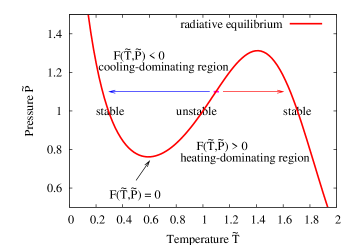
Figure 1: (Color online) Radiative-equilibrium curve (thick curve) of the Ginzburg-Landau-type heating-cooling function (16) in the $\widetilde{T}\widetilde{P}$ plane. The heating-cooling function $F$ equals zero on the curve. $a$, $b$, and $c$ in Eq. (16) are set to $1.0$, $2.0$, and $1.0$, respectively. The two arrows schematically denote that a small perturbation on an unstable state grows, and one of the stable two-phase states with lower or higher temperature on the radiative-equilibrium curve is finally realized.

Consider an optically thin neutral media with external heating and radiative cooling. Self-gravitation, magnetic field, and other body forces are neglected. The fluids are described through the following basic equations which include the laws of mass, momentum, and energy conservation, together with a perfect-gas equation of state:

$$\frac{\partial\rho}{\partial t}+\frac{\partial}{\partial x_{j}}(\rho u_{j})=0,$$ (1)

$$\frac{\partial}{\partial t}(\rho u_{i})+\frac{\partial}{\partial x_{j}}(\rho u_{i}u_{j}-\sigma_{ij})=-\frac{\partial P}{\partial x_{i}},$$ (2)

$$\frac{\partial E}{\partial t}+\frac{\partial}{\partial x_{j}}\left[(E+P)u_{j}-\sigma_{ij}u_{i}-K\frac{\partial T}{\partial x_{j}}\right]=-\rho{\cal L},$$ (3)

$$\sigma_{ij}=\mu\left[\left(\frac{\partial u_{i}}{\partial x_{j}}+\frac{\partial u_{j}}{\partial x_{i}}\right)\ -\frac{2}{3}\delta_{ij}\frac{\partial u_{k}}{\partial x_{k}}\right],$$ (4)

$$P=\frac{\rho k_{B}T}{m_{\mathrm{H}}}=nk_{B}T,$$ (5)

$$E\equiv\frac{P}{\gamma-1}+\frac{1}{2}\rho u_{i}^{2},$$ (6)

where $\rho$, $v$, $E$, and $P$ are density, velocity, total-energy density, and pressure, respectively. The thermal conductivity, the specific-heat ratio, and the viscosity coefficient are denoted by $K$, $\gamma$, and $\mu$, respectively. In general the thermal conductivity is a function of temperature but for simplicity we set it as a constant. $m_{\mathrm{H}}$ is the molecular mass of hydrogen and $k_{B}$ is the Boltzmann constant. ${\cal L}(T,P)$ is called a heating-cooling function, which describes the total of thermal input and output depending on temperature and pressure at each point. Note that fluids can be locally heated and cooled in this system since the fluids are sufficiently rarefied. Such fluids are common particularly in astrophysical systems.

We use the following non-dimensional equations derived from the original Eqs. (1)-(6):

$$\frac{\partial\widetilde{\rho}}{\partial\tau}+\frac{\partial}{\partial\widetilde{x}_{j}}(\widetilde{\rho}\widetilde{u}_{j})=0,$$ (7)

$$\frac{\partial}{\partial\tau}(\widetilde{\rho}\widetilde{u}_{i})+\frac{\partial}{\partial\widetilde{x}_{j}}\left(\widetilde{\rho}\widetilde{u_{i}}\widetilde{u_{j}}-\frac{\gamma-1}{\gamma}\frac{\Pr}{E_{p}}\widetilde{\sigma}_{ij}\right)=-\frac{\partial\widetilde{P}}{\partial\widetilde{x_{i}}},$$ (8)

$$Ep\left[\frac{1}{\gamma-1}\frac{\partial\widetilde{P}}{\partial\tau}+\frac{1}{\gamma-1}\frac{\partial}{\partial\widetilde{x}_{j}}(\widetilde{P}\widetilde{u}_{j})+\widetilde{P}\frac{\partial\widetilde{u}_{j}}{\partial\widetilde{x}_{j}}\right]-$$

$$\frac{\gamma-1}{\gamma}\Pr\widetilde{\sigma}_{ij}\frac{\partial\widetilde{u}_{i}}{\partial\widetilde{x}_{j}}-\frac{\partial^{2}\widetilde{T}}{\partial\widetilde{x}_{j}\partial\widetilde{x}_{j}}=-\widetilde{\rho}\widetilde{\cal L},$$ (9)

$$\widetilde{P}=\widetilde{\rho}\widetilde{T},$$ (10)

$$\widetilde{\sigma}_{ij}=\left[\left(\frac{\partial\widetilde{u}_{i}}{\partial\widetilde{x}_{j}}+\frac{\partial\widetilde{u}_{j}}{\partial\widetilde{x}_{i}}\right)-\frac{2}{3}\delta_{ij}\frac{\partial\widetilde{u}_{k}}{\partial\widetilde{x}_{k}}\right].$$ (11)

Here $\widetilde{x_{j}}=x_{j}/x_{0}$, $\widetilde{u_{j}}=u_{j}/u_{0}$, $\tau=t/(x_{0}/u_{0})$, $\widetilde{\rho}=\rho/\rho_{0}$, $\widetilde{T}=T/T_{0}$, $\widetilde{P}=P/P_{0}$, and $\widetilde{{\cal L}}={\cal L}/{\cal L}_{0}$, which are scaled by the corresponding characteristic values denoted by a subscript zero, respectively.

The characteristic length scale $x_{0}$ is defined as follows:

$$x_{0}=\sqrt{\frac{KT_{0}}{\rho_{0}{\cal L}_{0}}}.$$ (12)

This length is called Field length and represents the front width between two phases [20].

We set the characteristic velocity $u_{0}$ to be proportional to a sound speed:

$$u_{0}=\sqrt{\frac{k_{B}}{m_{\mathrm{H}}}T_{0}}.$$ (13)

There are two non-dimensional constants in the non-dimensional equations:

$$\Pr=\frac{\gamma}{\gamma-1}\frac{k_{B}\mu}{m_{\mathrm{H}}K},$$ (14)

$$Ep=\frac{1}{\rho_{0}{\cal L}_{0}}\frac{P_{0}}{t_{0}}.$$ (15)

$\Pr$ is called Prandtl number. $Ep$ represents the degree of thermal contribution to dynamics in Eq. (9). Larger $Ep$ induces slower dynamics in fluids.

In this paper, the following Ginzburg-Landau-type equation is adopted for the heating-cooling function [23, 13, 24]:

$$-\widetilde{\rho}\widetilde{\cal L}(\widetilde{T},\widetilde{P})=F(\widetilde{T},\widetilde{P})=a(\widetilde{T}-1)-b(\widetilde{T}-1)^{3}-c\ln\widetilde{P}.$$ (16)

We also tried the more realistic but complicated form of the heating-cooling function (17) used in astrophysical contexts [25, 26]:

$$\rho{\cal L}=-n\Gamma+n^{2}\Lambda(T),$$ (17)

$$\Gamma=2.0\times 10^{-26}\ \mathrm{ergs}\ \mathrm{s}^{-1},$$ (18)

$$\frac{\Lambda(T)}{\Gamma}= 1.0\times 10^{7}\exp[-1.184\times 10^{5}/(T+1000)]$$

$$+ 1.4\times 10^{-2}\sqrt{T}\exp(-92/T)\ \mathrm{cm}^{3}.$$ (19)

It is found that both the stationary solutions and the results of numerical simulations with the heating-cooling function (17) are qualitatively similar to those with the simplified heating-cooling function (16) (see Figs. 2,4 and Figs. 7,8). Therefore, for simplicity and for elucidation of fundamental mechanism, the simplest form of the heating-cooling function defined by Eq. (16) is adopted in this work.

In Fig. 1, we show a radiative equilibrium curve on which the heating-cooling function $F(\widetilde{T},\widetilde{P})$ is equal to zero. The S shape of the curve is essential to two-phase separation: supposed to a fixed pressure in a range with which the equation has three roots. Because two roots with high and low temperatures among them satisfy condition (20), they are stable against small temperature (density) perturbations,

$$\left(\frac{\partial F}{\partial\widetilde{T}}\right)_{\widetilde{P}}<0.$$ (20)

In contrast, the root with an intermediate temperature satisfies condition (21), and thus a small disturbance on the state grows. This instability is called thermal instability [20],

$$\left(\frac{\partial F}{\partial\widetilde{T}}\right)_{\widetilde{P}}>0.$$ (21)

Fluid particles around the unstable branch in Fig. 1 finally reach to each of stable branches with high or low temperatures via heating or cooling processes.

3 Pulselike stationary solutions

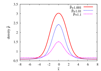
Figure 2: (Color online) Density profiles of pulselike stationary solutions for the three values of pressure $\widetilde{P}=1.1$, $1.01$, and $1.001$.

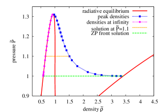
Figure 3: (Color online) Peak densities $\widetilde{\rho}_{0}$ and densities at infinity $\widetilde{\rho}_{\infty}$ of the pulselike stationary solutions. The dashed horizontal lines denote the projections of the solution with $\widetilde{P}=1.1$ and the ZP front solution with the saturation pressure $\widetilde{P}=1$.

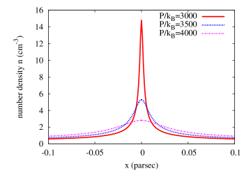
Figure 4: Pulselike stationary solutions obtained using the astrophysically realistic but complicated form (17).

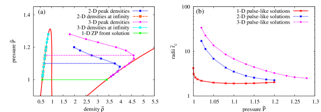
Figure 5: (a) Peak densities $\widetilde{\rho}_{0}$ and densities at infinity $\widetilde{\rho}_{\infty}$ of the pulselike stationary solutions of Eqs. (25)$-$(27) in two-dimensional and three-dimensional cases, respectively. The two-dimensional and three-dimensional densities at infinity almost overlap. The two dashed horizontal lines with $\widetilde{P}>1$ represent the projections of the density profiles of some two-dimensional and three-dimensional solutions into the $\widetilde{\rho}\widetilde{P}$ plane. The horizontal line with $\widetilde{P}=1$ represents the one-dimensional ZP front solution. (b) Radii of the pulselike stationary solutions as a function of pressure $\widetilde{P}$ in one-dimensional, two-dimensional axisymmetric, and three-dimensional spherically symmetric systems.

First, we will obtain stationary localized solutions of Eqs. (7)$-$(11). These are homoclinic orbits.

3.1 Plane-parallel geometry

Supposed that a fluid is stationary ($\partial/\partial\tau=0$ and $\widetilde{u}_{i}=0$), the governing equations are simplified in a plane-parallel geometry as follows:

$$F(\widetilde{T},\widetilde{P})+\frac{\partial^{2}\widetilde{T}}{\partial\widetilde{x}^{2}}=0,$$ (22)

$$\frac{\partial\widetilde{P}}{\partial\widetilde{x}}=0.$$ (23)

Because the pressure $\widetilde{P}$ becomes uniform via Eq. (23), the pressure works as a parameter in the temperature Eq. (22). Here for simplicity and for keeping the temperature positive, we set the parameters $a$, $b$, and $c$ of $F$ as 1, 2 and 1, respectively. However, note that transforming the variables as $\widetilde{x}=\sqrt{a}\xi$, $\widetilde{T}-1=\sqrt{a/b}\hat{T}$, and $\widetilde{P}=\hat{P}^{\sqrt{ab}/c}$, the parameters can be eliminated from Eq. (22).

We impose the following boundary conditions in the semi-infinite space ($0\leq\widetilde{x}<\infty$):

$$\frac{\partial\widetilde{T}}{\partial\widetilde{x}}=0\hskip 20.0pt(\widetilde{x}=0,\ \widetilde{x}\to\infty).$$ (24)

Since Eq. (22) is a second-order ordinary differential equation with respect to $\widetilde{x}$, the two boundary conditions in Eq. (24) uniquely determine the solution $\widetilde{T}(\widetilde{x})$ if it exists. Simultaneously, the values of temperature at the boundaries, i.e., $\widetilde{T}_{0}=\widetilde{T}(\widetilde{x}=0)$ and $\widetilde{T}_{\infty}=\widetilde{T}(\widetilde{x}\to\infty)$, are given. We numerically solve Eq. (22) with the boundary conditions (24) by means of a shooting method, and we obtain $\widetilde{T}(\widetilde{x})$ and also $\widetilde{T}_{0}$ and $\widetilde{T}_{\infty}$ for various values of pressure. In Fig. 2, we show the density profiles $\widetilde{\rho}(\widetilde{x})=\widetilde{P}/\widetilde{T}(\widetilde{x})$ of the solutions for three values of pressure $\widetilde{P}=1.1$, $1.01$, and $1.001$. By the reflection symmetry of Eq. (22) the solutions are extended to $\widetilde{x}<0$. These localized cold solutions are called pulselike stationary solutions, hereafter. Figure 3 shows the peak density $\widetilde{\rho}_{0}=\widetilde{P}/\widetilde{T}_{0}$ and the density at infinity $\widetilde{\rho}_{\infty}=\widetilde{P}/\widetilde{T}_{\infty}$ as a function of pressure $\widetilde{P}$. Note that the peak densities are always lower than the density of the stable equilibrium state and apart from the radiative-equilibrium curve ($F=0$) when $\widetilde{P}>1$. As $\widetilde{P}\to 1+$, the peak density asymptotically approaches one of the stable radiative equilibriums, and the pulselike solution becomes the ZP solution (front solution).

We also obtained pulselike stationary solutions using the realistic but complicated form of heating-cooling function. The solutions are shown in Fig. 4. With the respect that the solutions are also homoclinic orbits, they are qualitatively similar to those obtained with simplified heating-cooling function (16) as shown in Fig. 2. This supports the use of the simplified heating-cooling function (16).

3.2 Axisymmetric and spherically-symmetric geometry

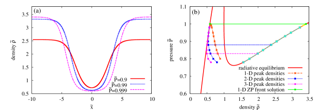
Figure 6: (Color online) (a) Density profiles of the warm pulselike stationary solutions of Eqs. (22) and (24) for the three values of pressure $\widetilde{P}=0.9$, $0.99$, and $0.999$. (b) Peak densities of the solutions in one-dimensional, two-dimensional axisymmetric, and three-dimensional spherically symmetric systems in the $\widetilde{\rho}\widetilde{P}$ plane. The two horizontal lines with $\widetilde{P}<1$ represent the projections of the density profiles of some two-dimensional and three-dimensional solutions into the $\widetilde{\rho}\widetilde{P}$ plane. The horizontal line with $\widetilde{P}=1$ represents the one-dimensional ZP front solution.

We also obtain pulselike stationary solutions in multidimensional systems as in the one-dimensional case. We suppose that the systems are axisymmetric in two-dimensional cases and spherically symmetric in three-dimensional cases. These symmetries make the governing equations simpler as follows:

$$F(\widetilde{T},\widetilde{P})+\frac{d-1}{\widetilde{r}}\frac{\partial\widetilde{T}}{\partial\widetilde{r}}+\frac{\partial^{2}\widetilde{T}}{\partial\widetilde{r}^{2}} = 0,$$ (25)

$$\frac{\partial\widetilde{P}}{\partial\widetilde{r}} = 0,$$ (26)

where $\widetilde{r}$ and $d$ are the radial coordinate and the space dimension, respectively. The boundary conditions are imposed as follows:

$$\frac{\partial\widetilde{T}}{\partial\widetilde{r}}=0\hskip 20.0pt(\widetilde{r}=0,\widetilde{r}\to\infty).$$ (27)

These equations are numerically solved by means of the shooting method. As in the case of the one-dimensional system, we obtain a localized solution $\widetilde{\rho}(\widetilde{r})=\widetilde{P}/\widetilde{T}(\widetilde{r})$ with peak density $\widetilde{\rho}_{0}$ at the origin and density at infinity $\widetilde{\rho}_{\infty}$ at $\widetilde{r}\to\infty$. The two densities are dependent only on pressure. Figure 5(a) shows $\widetilde{\rho}_{0}$ and $\widetilde{\rho}_{\infty}$ as a function of pressure $\widetilde{P}$ for the two-dimensional and three-dimensional solutions. As pressure increases from the saturation pressure $\widetilde{P}=1$, the peak density leaves away from the radiative-equilibrium curve. Note that by the curvature effect represented by the second term in the left-hand side of Eq. (25), the peak density increases along with the radiative-equilibrium curve as pressure increases, unlike the one-dimensional solution in Fig. 3.

We define the size of the localized structures as a radius $\widetilde{r}_{c}$, which satisfies $\widetilde{T}(\widetilde{r}_{c})=(\widetilde{T}_{0}+\widetilde{T}_{\infty})/2$. Figure 5(b) shows the radii as a function of pressure. When $\widetilde{P}\to 1+$, the radii go to infinity. Since the curvature term of Eq. (25) asymptotically approaches zero in the limit, the localized solutions then lead to the ZP front solution in a plane-parallel geometry. The dependence of the cloud size on pressure qualitatively agrees with the results of Nagashima et al. [17].

3.3 Bubble solutions

Warm, rarefied, and localized structures surrounded by cold dense media are also numerically obtained in the same way as the cold structures obtained in Sec. 3.2. The density profiles of the solutions for the three values of pressure $\widetilde{P}=0.9$, $0.99$, and $0.999$ are shown in Fig. 6(a). These structures are realized only when $\widetilde{P}<1$. Figure 6(b) shows the peak densities $\widetilde{\rho}_{0}$ and densities at infinity $\widetilde{\rho}_{\infty}$ as a function of pressure $\widetilde{P}$. As in the case of the cold structures, the peak densities are apart from the radiative-equilibrium curve when pressure gets smaller than the saturation pressure $\widetilde{P}=1$. In the limit that $\widetilde{P}\to 1-$, the solutions approach the one-dimensional ZP front solution corresponding to a plane-parallel and localized warm structure of an infinity size. These localized warm solutions are called ”bubbles” [14, 9] and have been frequently referred in astrophysical contexts [9].

4 relaxation process of localized cold structures

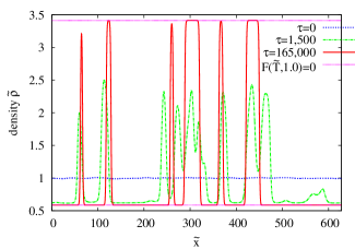
Figure 7: (Color online) The two-phase separation from the random small density disturbance around $\widetilde{\rho}=1$. The density profiles at $\tau=0$, $1500$ and $165000$ are shown. The times correspond to the initial, transient, and quasistationary state, respectively. The two horizontal lines represent the densities of the states of the radiative equilibrium with the saturation pressure $\widetilde{P}=1$.

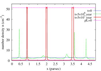
Figure 8: (Color online) Formation process of localized structures in direct numerical simulation with the astrophysically realistic heating-cooling function (17). The density profiles at the three times $t=0$, $5.0\times 10^{6}\;\mathrm{year}$, and $5.0\times 10^{7}\;\mathrm{year}$ are plotted. The two horizontal lines represent the densities of the states of the radiative equilibrium at the saturation pressure.

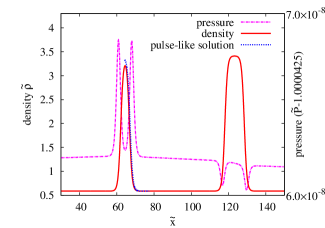
Figure 9: (Color online) Density and pressure profiles at $\tau=165000$ in the quasistationary state. The pulselike stationary solution with the pressure value at the coordinate where the localized structure has a peak density is superposed.

We investigate the role of the cold pulselike stationary solutions in the formation of localized structures by direct numerical simulations. Equations (7)-(11) are numerically solved in a plane-parallel geometry with 8192 grids and a periodic boundary condition. We use a high-accuracy pseudospectral method partially dealiased and a fourth-order Runge-Kutta method. As initial conditions, pressure is set to the saturation pressure and velocity is zero, that is, $\widetilde{P}=1$ and $\widetilde{u}=0$. Density is a small random disturbance consisting of only low wave-number modes ($k\leq 16$) added to a homogeneous state $\widetilde{\rho}=1$ that is on the unstable branch of the radiative-equilibrium curve (see Fig. 1). We set non-dimensional constants $Ep$ and $\Pr$ to $1.0\times 10^{2}$ and $1.0$, respectively. Koyama and Inutsuka used $Ep\simeq 64$ in a realistic situation so that $Ep=100$ seems to be a feasible value. The specific-heat ratio $\gamma$ is set to 5/3.

Figure 7 shows a formation process of localized structures. The initial density disturbance rapidly grows and evolves into warm and cold regions due to a thermal instability. Some of the cold regions merge successively and some of them evaporate in the evolution. Several localized cold structures finally survive in warm media, and then these structures persist for a long time. Because most of the kinetic energy in the whole system is lost during the two-phase separation, the cold structures are almost stationary.

For comparison, we also have numerically calculated the two-phase separation with the realistic but complicated form of heating-cooling function (17) and original astrophysical Eqs. (1)$-$(6). Some of the results are shown in Fig. 8. The relaxation process is qualitatively similar to that with simplified heating-cooling function (16) shown in Fig. 7. Some of the cold regions merge and evaporate, and some localized structures finally survive in the process.

To examine the decaying process of localized structures in detail, we focus on two typical localized cold structures. One with a longer lifetime is seen around $x\sim 60$ in Fig. 7. The peak density of this localized structure does not yet attain the value of the density in the radiative equilibrium ($F=0$). However, as seen in Fig. 9, the localized cold structure is quite similar in form to a pulselike stationary solution with the value of pressure at the peak of the localized structure. The values of pressure at the peak of localized structures are called peak pressure. Note that in Fig. 9 the value of pressure is subtracted by 1.000 042 5 so that the pressure variation around the peak of the localized structure is negligible and does not affect the estimation of the peak pressure.

The peak density of the localized structures decreases slowly and monotonically by evaporation and they finally disappear. We estimate the characteristic time of the decaying process, i.e., the evaporation time of the localized structures. In Fig. 10, we show the evolution of the peak density of the localized structures obtained in two runs under the same conditions except for the initial condition: one with a longer lifetime is called LS1 and the other LS2 hereafter. The evolution is separated into two periods: the fast transient one and the slow decay one. We call the latter a quasistationary state. The transient period finishes at around $\tau=2.0\times 10^{3}$. This time corresponds to a sound crossing time defined as a time during which a sound wave passes through the system.

The decay curves of the peak density after attaining the quasistationary state are well fitted by a double-exponential function $A\exp\{-B\exp[(\tau-\tau_{0})/\tau_{c}]\}$ as shown in the inset of Fig. 10; the values of the fitting parameters of LS1 are $A=3.27$, $B=1.24\times 10^{-2}$, $\tau_{0}=45000$, and $\tau_{c}=2.91\times 10^{5}$ for $4.5\times 10^{4}\leq\tau\leq 1.6\times 10^{5}$; those of LS2 for $4.5\times 10^{4}\leq\tau\leq 1.1\times 10^{5}$ are $A=2.95$, $B=1.07\times 10^{-2}$, $\tau_{0}=45000$, and $\tau_{c}=2.21\times 10^{4}$. The latter case shows that the late decaying process is faster than a double-exponential function, but the characteristic time estimated is shorter than the period of the saturation process $1.2\times 10^{5}$. In this sense, the characteristic time gives a good estimate of the evaporation time of the localized structure.

It should be noted that the relaxation times $\tau_{c}$ are much longer than the sound crossing time. In Sec. 5, we discuss the details of this decaying process of the peak density.

5 persistence of pulselike clouds with viscosity

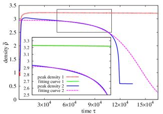
Figure 10: (Color online) Peak density evolutions of the localized structure at $\widetilde{x}\sim 60$ in Fig. 7 and the other localized structure derived by another run. Inset: the peak density evolutions magnified in the quasistationary state $4.5\times 10^{4}\leq\tau\leq 1.1\times 10^{5}$. The curve with the larger peak density is fitted by the double-exponent function defined as $A\exp\{-B\exp[(\tau-\tau_{0})/\tau_{c}]\}$ with $A=3.27$, $B=1.24\times 10^{-2}$, and the relaxation time $\tau_{c}=2.91\times 10^{5}$. The curve with the smaller peak density is fitted by the above double-exponent function with $A=2.95$, $B=1.07\times 10^{-2}$, and $\tau_{c}=2.21\times 10^{4}$.

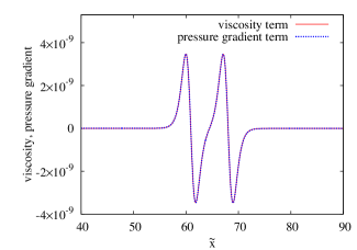
Figure 11: (Color online) The viscosity term and the pressure-gradient term of the kinetic Eq. (8) in the quasistationary state with Prandtl number $\Pr=1.0$ for LS1 at $\tau=165000$.

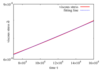
Figure 12: (Color online) The time evolution of the viscous stress $\widetilde{\sigma}$. The curve is fitted by an exponential function: $\sigma_{0}\exp((\tau-\tau_{0})/\tau_{c\sigma})$, where $\tau_{0}=70000$, $\sigma_{0}=6.20\times 10^{-8}$, and $\tau_{c\sigma}=3.63\times 10^{5}$.

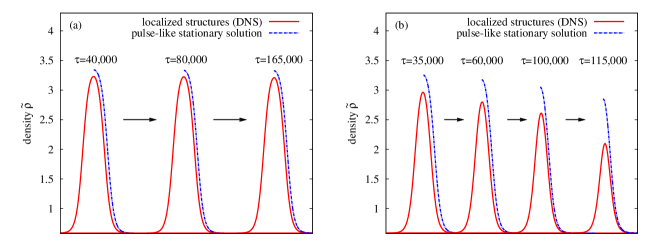
Figure 13: (Color online) Comparison of localized structures and corresponding pulselike stationary solutions in the relaxation process shown in Fig. 10: (a) LS1 and (b) LS2. The value of pressure of the pulselike solutions is set to the peak pressure of the localized structure at each time.

Why can the localized cold structures be sustained extremely longer than expected? Here we focus on viscosity, although the viscosity has been omitted in most of the previous studies. Since we have performed numerical simulations with a high-accuracy spectral scheme, we can deal with the viscosity more precisely than the previous studies.

Figure 11 shows the viscosity term and the pressure-gradient term of the kinetic equation (8) around the localized structure in the quasistationary state $\tau=165000$. While the pressure is almost uniform because of the mixing by sound waves, a weak pressure gradient is maintained around localized structures (see also Fig. 9). Moreover, the weak pressure gradient almost coincides with the viscosity. This balance between the viscosity and the pressure gradient causes the persistence of the localized structure. To see this in detail, we rewrite the basic equations (7) and (8) in a plane-parallel geometry as follows:

$$\frac{D\widetilde{\rho}}{D\tau}=-\frac{3}{4}\widetilde{\sigma}\widetilde{\rho},$$ (28)

$$\frac{D\widetilde{\sigma}}{D\tau}+\frac{3}{4}\widetilde{\sigma}^{2}=\left(\frac{4}{3}\frac{1}{\widetilde{\rho}}\frac{\partial}{\partial\widetilde{x}}-\frac{4}{3}\frac{1}{\widetilde{\rho}^{2}}\frac{\partial\widetilde{\rho}}{\partial\widetilde{x}}\right)\left(\frac{\gamma-1}{\gamma}\frac{\Pr}{Ep}\frac{\partial\widetilde{\sigma}}{\partial\widetilde{x}}-\frac{\partial\widetilde{P}}{\partial\widetilde{x}}\right),$$ (29)

where $D/D\tau=\partial/\partial\tau+\widetilde{v}\partial/\partial\widetilde{x}$ is a Lagrangian derivative. $\widetilde{\sigma}=4/3(\partial\widetilde{v}/\partial\widetilde{x})$ is a viscous stress, which represents the degree of compressibility.

Figure 12 shows that the viscous stress $\widetilde{\sigma}$ exponentially grows in the quasistationary state. Hence, the Lagrangian time derivative $D\widetilde{\sigma}/D\tau$ can be written as $\alpha\widetilde{\sigma}$, where the growth rate is $\alpha\sim 10^{-6}$. The very small growth rate is just caused by the small difference between the viscosity and the pressure gradient in Eq. (29) when the nonlinear term in the left-hand side is negligible. In fact $\widetilde{\sigma}\gg\alpha\widetilde{\sigma}\gg\widetilde{\sigma}^{2}$ since the viscous stress $\widetilde{\sigma}$ is the order of $10^{-8}$ as seen in Fig. 12. The slow exponential growth of the viscous stress finally leads to the double-exponential decay with a long relaxation time via Eq. (28).

In this relaxation process, as shown in Fig. 13, the localized structures remain close to pulselike stationary solutions. The balance fixes the peak pressure of the localized structure. Then the structure is attracted and trapped to one of the pulselike stationary solutions with the corresponding pressure value that seems to behave similar to a saddlelike fixed point in the phase space. The deviation of the localized structure from the pulselike stationary solution induces both the small pressure gradient and viscous effect (see Fig. 11). Finally the two effects induced balance to each other and then this balance suppresses the induction of flow that transfers heat and material from localized structures.

The one-dimensional Eqs. (28) and (29) can be extended to multidimensional equations as follows:

$$\frac{D\tilde{\rho}}{D\tau}=-(\mathrm{div}\,{\bm{\tilde{}}{u}})\tilde{\rho},$$ (30)

$$\frac{D(\mathrm{div}\,{\bm{\tilde{}}{u}})}{D\tau}+\frac{\partial\tilde{u}_{j}}{\partial\tilde{x}_{i}}\frac{\partial\tilde{u}_{i}}{\partial\tilde{x}_{j}}=$$

$$\left(\frac{1}{\tilde{\rho}}\frac{\partial}{\partial\tilde{x}_{i}}-\frac{1}{\tilde{\rho}^{2}}\frac{\partial\tilde{\rho}}{\partial\tilde{x}_{i}}\right)\left(\frac{\gamma-1}{\gamma}\frac{Pr}{Ep}\frac{\partial\tilde{\sigma}_{ij}}{\partial\tilde{x}_{j}}-\frac{\partial\tilde{P}}{\partial\tilde{x}_{i}}\right).$$ (31)

These equations suggest that the balance between the viscosity and the pressure gradient plays a crucial role in the relaxation of the multidimensional localized structures through the divergence of velocity. Therefore, the viscosity should be considered as well as the pressure gradient regardless of the dimension of the system.

6 Discussion and concluding remarks

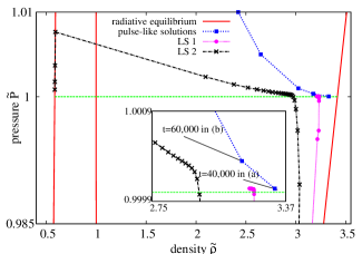
Figure 14: (Color online) Evolutions of peak pressure and peak density of the localized structures LS1 and LS2 shown in Fig. 10. The equilibrium curve and the pulselike stationary solution illustrated in Fig. 3 are also drawn. The points on the evolution curves are plotted every $5000$ from $\tau=5000$ to $\tau=165000$ for LS1 and from $\tau=5000$ to $\tau=135000$ for LS2. Inset: the evolutions of peak pressure and peak density magnified around the times in which the localized structures are trapped near the corresponding pulselike stationary solutions.

We have investigated localized cold structures in thermally unstable two-phase fluids. The two-phase separation is induced by thermal instability via local heating and cooling described by the Ginzburg-Landau-type heating-cooling function. We have numerically obtained pulselike stationary solutions of which the peak densities are not in the states of the radiative equilibrium in one-dimensional, two-dimensional axisymmetric, and three-dimensional spherically symmetric systems using a shooting method. Our solutions differ from the solutions obtained in the previous studies which consider bistable media and fronts connecting the two stable states [13, 14, 27]. The size of the solutions depends only on pressure, and the relationship between the size and the pressure qualitatively coincides with the results of Nagashima et al. [17].

We have carried out direct numerical simulations of the thermally unstable fluids with a small random density perturbation using a high-accuracy spectral method. During the two-phase separation, many cold clouds are formed, and some of them merge or evaporate. Finally, several cold clouds are left in the warm media and persist for a long time. The pulselike stationary solutions obtained by the shooting method are actually observed in the direct numerical simulations. Such small and long-lived clouds have been observed in interstellar media and might be related with the long-lived localized clouds we have found [17, 15, 16].

We have shown that the viscosity balances with the pressure gradient in the quasistationary state at higher order. The balance remarkably suppresses the evaporation of the localized clouds. Note that the viscous and the pressure-gradient effects are very weak but play a crucial role in the persistence of the structures. In contrast, most of the previous studies have neglected the viscous effect (e.g., Refs. [13, 14, 27, 17, 28]). Our results strongly suggest that the viscosity changes the relaxation process and suppresses the evaporation of the cold clouds. We, therefore, expect that multidimensional clouds, which are also pulselike as the one-dimensional clouds, have a long relaxation time because of the viscosity.

Although the pulselike stationary solutions are obtained under constant pressure, the pressure is a dependent variable in direct numerical simulations. However, the balance between the viscosity and the pressure gradient tends to keep the pressure nearly constant (pressure saturation). In this situation, one of the pulselike stationary solutions is selected and attracts the localized structure. This solution behaves similar to a saddlelike fixed point in phase space. Figure 14 shows the evolution of peak values of the localized structures LS1 and LS2 in density-pressure space. The peak pressure and density of the localized structure approach those of the pulselike stationary solution. After a long stay around there, it quickly leaves from there to the lower equilibrium state. Note that the leaving process of LS1 is not seen in Fig. 14. In this final escaping process, the profile of the localized structure quickly deviates from the pulselike stationary solution with the same pressure value as the peak pressure of the localized structure (see Fig. 13). By this picture of the relaxation process, the relaxation time might be dependent on the approaching process along with a stable manifold of the pulselike stationary solution. When similar to the case of LS2, the pressure saturation is not sufficient, that is, localized structures are not close enough to the stable manifold of one of the pulselike stationary solutions, the localized structures seem to approach a part of a manifold formed by the pulselike stationary solutions rather than a single one, i.e., a fixed point. Anyway, the dynamical system approach will help us understand the formation process of localized clouds.

In the future, we plan to perform direct numerical simulations in two-dimensional axisymmetric and three-dimensional spherically symmetric systems in order to confirm the persistence of the multidimensional localized structures with the viscosity. In addition, we will employ two-dimensional full numerical simulations in order to investigate multidimensional effects such as interface dynamics.

Acknowledgement: We would like to acknowledge stimulating discussions with Tsuyoshi Inoue and Shu-ichiro Inutsuka. This work was supported by the Grant-in-Aid for the Global COE Program ”The Next Generation of Physics, Spun from Universality and Emergence” from the Ministry of Education, Culture, Sports, Science and Technology (MEXT) of Japan. The numerical calculations were carried out on SX8 at YITP in Kyoto University and scholar-processors at RIMS in Kyoto University. S.T. was partly supported by the Grant-in-Aid for Scientific Research (C)(Grant No. 18540373) from the Japan Society for the Promotion of Science.

References

- [1] S. Toh. Statistical model with localized structures describing the spatio-temporal chaos of kuramoto-sivashinsky equation. J. Phys. Soc. Jpn, 56:949, 1987.
- [2] H. Iwasaki and S. Toh. Statistics and structures of strong turbulence in a complex ginzburg-landau equation. Prog. Theor. Phys., 87:1127, 1992.
- [3] T. Itano and S. Toh. The dynamics of bursting process in wall turbulence. J. Phys. Soc. Jpn, 61:703, 2001.
- [4] G. Kawahara and S. Kida. Periodic motion embedded in plane couette turbulence: regeneration cycle and burst. J. Fluid Mech., 449:291, 2001.
- [5] B. Eckhardt, T. M. Schneider, B. Hof, and J. Westerweel. Turbulence transition in pipe flow. Ann. Rev. Fluid Mech., 39:447, 2007.
- [6] F. Waleffe. Homotopy of exact coherent structures in plane shear flows. Phys. Fluids, 15:1517, 2003.
- [7] K. Davidson. Photoionization and the emission-line spectra of quasi-stellar objects. Astrophys. J., 171:213, 1972.
- [8] B. Lipschultz. Review of marfe phenomenas in tokamaks. J. Nucl. Mater., 145-147:15, 1987.
- [9] B. Meerson. Nonlinear dynamics of radiative condensations in optically thin plasmas. Rev. Mod. Phys., 68:215, 1996.
- [10] E. Audit and P. Hennebelle. Thermal condensation in a turbulent atomic hydrogen flow. Astron. Astrophys., 433:1, 2005.
- [11] F. Heitsch, A. Burkert, L. W. Hartmann, A. D. Slyz, and J. E. G. Devriendt. Formation of structure in molecular clouds: A case study. Astrophys. J. Lett., 633:L113, 2005.
- [12] E. Vázquez-Semadeni, D. Ryu, T. Passot, R. F. González, and A. Gazol. Molecular cloud evolution. I. molecular cloud and thin cold neutral medium sheet formation. Astrophys. J., 643:245, 2006.
- [13] C. Elphick, O. Regev, and N. Shaviv. Dynamics of fronts in thermally bistable fluids. Astrophys. J., 392:106, 1992.
- [14] I. Aranson, B. Meerson, and P. V. Sasorov. Nonlinear radiative-condensation instability and pattern formation: One-dimensional dynamics. Phys. Rev. E, 47:4337, 1993.
- [15] R. Braun and N. Kanekar. Tiny h i clouds in the local ism. Astron. Astrophys. Lett., 436:L53, 2005.
- [16] S. Stanimirović and C. Heiles. The thinnest cold h i clouds in the diffuse interstellar medium? Astrophys. J., 631:371, 2005.
- [17] M. Nagashima, S. Inutsuka, and H. Koyama. How long can tiny hi clouds survive ? Astrophys. J. Lett., 652:L41, 2006.
- [18] E. N. Parker. Instability of thermal fields. Astrophys. J., 117:431, 1953.
- [19] G. B. Field, D. W. Goldsmith, and H. J. Habing. Cosmic-ray heating of the interstellar gas. Astrophys. J. Lett., 155:L149, 1969.
- [20] G. B. Field. Thermal instability. Astrophys. J., 142:531, 1965.
- [21] Y. B. Zel’dovich and S. B. Pikel’ner. The phase equilibrium and dynamics of a gas volume that is heated and cooled. Sov. Phys. JETP, 29:170, 1969.
- [22] R. Graham and W. D. Langer. Pressure equilibrium of finite-size clouds in the interstellar medium. Astrophys. J., 179:469, 1973.
- [23] C. Elphick, O. Regev, and E. A. Spiegel. Complexity from thermal instability. Mon. Not. R. Astron. Soc., 250:617, 1991.
- [24] M. Nagashima, H. Koyama, and S. Inutsuka. Evaporation and condensation of hi clouds in thermally bistable interstellar media: semi-analytic description of isobaric dynamics of curved interfaces. Mon. Not. R. Astron. Soc. Lett., 361:L25, 2005.
- [25] H. Koyama and S. Inutsuka. Molecular cloud formation in shock-compressed layers. Astrophys. J., 532:980, 2000.
- [26] H. Koyama and S. Inutsuka. An origin of supersonic motions in interstellar clouds. Astrophys. J. Lett., 564:L97, 2002.
- [27] N. J. Shaviv and O. Regev. Interface dynamics and domain growth in thermally bistable fluids. Phys. Rev. E, 50:2048, 1994.
- [28] T. Inoue, S. Inutsuka, and H. Koyama. Structure and stability of phase transition layers in the interstellar medium. Astrophys. J., 652:1331, 2006.