Q-CSMA: Queue-Length Based CSMA/CA Algorithms for Achieving Maximum Throughput and Low Delay in Wireless Networks

Abstract

Recently, it has been shown that CSMA-type random access algorithms can achieve the maximum possible throughput in ad hoc wireless networks. However, these algorithms assume an idealized continuous-time CSMA protocol where collisions can never occur. In addition, simulation results indicate that the delay performance of these algorithms can be quite bad. On the other hand, although some simple heuristics (such as distributed approximations of greedy maximal scheduling) can yield much better delay performance for a large set of arrival rates, they may only achieve a fraction of the capacity region in general. In this paper, we propose a discrete-time version of the CSMA algorithm. Central to our results is a discrete-time distributed randomized algorithm which is based on a generalization of the so-called Glauber dynamics from statistical physics, where multiple links are allowed to update their states in a single time slot. The algorithm generates collision-free transmission schedules while explicitly taking collisions into account during the control phase of the protocol, thus relaxing the perfect CSMA assumption. More importantly, the algorithm allows us to incorporate mechanisms which lead to very good delay performance while retaining the throughput-optimality property. It also resolves the hidden and exposed terminal problems associated with wireless networks.

I Introduction

For wireless networks with limited resources, efficient resource allocation and optimization (e.g., power control, link scheduling, routing, congestion control) play an important role in achieving high performance and providing satisfactory quality-of-service (QoS). In this paper, we study link scheduling (or Media Access Control, MAC) for wireless networks, where the links (node pairs) may not be able to transmit simultaneously due to transceiver constraints and radio interference. A scheduling algorithm (or MAC protocol) decides which links can transmit data at each time instant so that no two active links interfere with each other.

The performance metrics of interest in this paper are throughput and delay. The throughput performance of a scheduling algorithm is often characterized by the largest set of arrival rates under which the algorithm can keep the queues in the network stable. The delay performance of a scheduling algorithm can be characterized by the average delay experienced by the packets transmitted in the network. Since many wireless network applications have stringent bandwidth and delay requirements, designing high-performance scheduling algorithms to achieve maximum possible throughput and low delay is of great importance, which is the main objective of this paper. We also want the scheduling algorithms to be distributed and have low complexity/overhead, since in many wireless networks there is no centralized entity and the resources at the nodes are very limited.

It is well known that the queue-length based Maximum Weight Scheduling (MWS) algorithm is throughput-optimal [26], in the sense that it can stabilize the network queues for all arrival rates in the capacity region of the network (without explicitly knowing the arrival rates). However, for general interference models MWS requires the network to solve a complex combinatorial optimization problem in each time slot and hence, is not implementable in practice.

Maximal scheduling is a low-complexity alternative to MWS but it may only achieve a small fraction of the capacity region [6, 29]. Greedy Maximal Scheduling (GMS), also known as Longest-Queue-First (LQF) Scheduling, is another natural low-complexity alternative to MWS which has been observed to achieve very good throughput and delay performance in a variety of wireless network scenarios. GMS proceeds in a greedy manner by sequentially scheduling a link with the longest queue and disabling all its interfering links. It was shown in [7] that if the network satisfies the so-called local-pooling condition, then GMS is throughput-optimal; but for networks with general topology GMS may only achieve a fraction of the capacity region [14, 16, 30]. Moreover, while the computational complexity of GMS is low, the signaling and time overhead of decentralization of GMS can increase with the size of the network [16].

Another class of scheduling algorithms are CSMA (Carrier Sense Multiple Access) type random access algorithms. Under CSMA, a node (sender of a link) will sense whether the channel is busy before it transmits a packet. When the node detects that the channel is busy, it will wait for a random backoff time. Since CSMA-type algorithms can be easily implemented in a distributed manner, they are widely used in practice (e.g., the IEEE 802.11 MAC protocol). In [4] the authors derived an analytical model to calculate the throughput of a CSMA-type algorithm in multi-hop wireless networks. They showed that the Markov chain describing the evolution of schedules has a product-form stationary distribution under an idealized continuous-time CSMA protocol (which assumes zero propagation/sensing delay and no hidden terminals) where collisions can never occur. Then the authors proposed a heuristic algorithm to select the CSMA parameters so that the link service rates are equal to the link arrival rates which were assumed to be known. No proof was given for the convergence of this algorithm. This model was used in [27] to study throughput and fairness issues in wireless ad hoc networks. The insensitivity properties of such a CSMA algorithm have been recently studied in [17].

Based on the results in [4, 27, 17], a distributed algorithm was developed in [12] to adaptively choose the CSMA parameters to meet the traffic demand without explicitly knowing the arrival rates. The results in [12] make a time-scale separation assumption, whereby the CSMA Markov chain converges to its steady-state distribution instantaneously compared to the time-scale of adaptation of the CSMA parameters. Then the authors suggested that this time-scale separation assumption can be justified using a stochastic-approximation type argument which was verified in [19, 11]. Preliminary ideas for a related result was reported in [23], where the authors study distributed algorithms for optical networks. But it is clear that their model also applies to wireless networks with CSMA. In [24], a slightly modified version of the algorithm proposed in [23] was shown to be throughput-optimal. The key idea in [24] is to choose the link weights to be a specific function of the queue lengths to essentially separate the time scales of the link weights and the CSMA dynamics. Further, the results in [24] assume that the max-queue-length in the network is known which is estimated via a distributed message-passing procedure. Similar modifications to 802.11 have been studied in [1, 28] where the back-pressure on a link is used as the weight instead of the queue length.

While the results in our paper are most closely related to the works in [4, 12, 24], we also note important contributions in [5, 8, 20, 22] which make connections between random access algorithms and stochastic loss networks.

Although the recent results on CSMA-type random access algorithms show throughput-optimality, simulation results indicate that the delay performance of these algorithms can be quite bad and much worse than MWS and GMS. Thus, one of our goals in this paper is to design distributed scheduling algorithms that have low complexity, are provably throughput-optimal, and have good delay performance. Towards this end, we design a discrete-time version of the CSMA random access algorithm. It is based on a generalization of the so-called Glauber dynamics from statistical physics, where multiple links are allowed to update their states based on their queue lengths in a single time slot. Our algorithm generates collision-free data transmission schedules while allowing for collisions during the control phase of the protocol (as in the 802.11 MAC protocol), thus relaxing the perfect CSMA assumption of the algorithms studied in [4, 12, 24]. Our approach to modeling collisions is different from the approaches in [13, 19]. In [19] the authors pointed out that, as the transmission probabilities are made small and the transmission lengths are made large, their discrete-time model approximates the continuous-time model with Poisson clocks, but it is difficult to quantify the throughput difference between these two models. The algorithm in [13] places upper bounds on the CSMA parameters, while the loss in throughput due to this design choice is also hard to quantify. Instead, we directly quantify the loss in throughput as the ratio of the duration of the control slot to the duration of the data slot (see Remark 1 in Section IV). More importantly, our formulation allows us to incorporate delay-reduction mechanisms in the choice of schedules while retaining the algorithm’s throughput-optimality property. It also allows us to resolve the hidden and exposed terminal problems associated with wireless networks [2].

We organize the paper as follows. In Section II we introduce the network model. In Section III we present the basic scheduling algorithm and show that the (discrete-time) Markov chain of the transmission schedules has a product-form distribution. In Section IV we present a distributed implementation of the basic scheduling algorithm, called Q-CSMA (Queue-length based CSMA/CA). In Section V we propose a hybrid Q-CSMA algorithm which combines Q-CSMA with a distributed procedure that approximates GMS to achieve both maximum throughput and low delay. We evaluate the performance of different scheduling algorithms via simulations in Section VI. The paper is concluded in Section VII.

II Network Model

We model a (single-channel) wireless network by a graph $G=(V,E)$, where $V$ is the set of nodes and $E$ is the set of links. Nodes are wireless transmitters/receivers. There exists a directed link $(n,m)\in E$ if node $m$ can hear the transmission of node $n$. We assume that if $(n,m)\in E$, then $(m,n)\in E$.

For any link $i\in E$, we use $\mathcal{C}(i)$ to denote the set of conflicting links (called conflict set) of $i$, i.e., $\mathcal{C}(i)$ is the set of links such that if any one of them is active, then link $i$ cannot be active. The conflict set $\mathcal{C}(i)$ may include

• Links that share a common node with link $i$. This models the node-exclusive constraint where two links sharing a common node cannot be active simultaneously.

• Links that will cause interference to link $i$ when transmitting. This models the radio interference constraint where two links that are close to each other cannot be active simultaneously.

We assume symmetry in the conflict set so that if $i\in\mathcal{C}(j)$ then $j\in\mathcal{C}(i)$.

We consider a time-slotted system. A feasible (collision-free) schedule of $G=(V,E)$ is a set of links that can be active at the same time according to the conflict set constraint, i.e., no two links in a feasible schedule conflict with each other. We assume that all links have unit capacity, i.e., an active link can transmit one packet in one time slot under a feasible schedule. Note that the results in this paper can be readily extended to networks with arbitrary link capacities.

A schedule is represented by a vector $\mathbf{x}\in\{0,1\}^{|E|}$. The $i^{\rm th}$ element of $\mathbf{x}$ is equal to $1$ (i.e., $x_{i}=1$) if link $i$ is included in the schedule; $x_{i}=0$ otherwise. With a little bit abuse of notation, we also treat $\mathbf{x}$ as a set and write $i\in\mathbf{x}$ if $x_{i}=1$. Note that a feasible schedule $\mathbf{x}$ satisfies the following condition:

$$x_{i}+x_{j}\leq 1,\mbox{ for all }i\in E\mbox{ and }j\in\mathcal{C}(i).$$ (1)

Let $\mathcal{M}$ be the set of all feasible schedules of the network.

A scheduling algorithm is a procedure to decide which schedule to be used (i.e., which set of links to be activated) in every time slot for data transmission. In this paper we focus on the MAC layer so we only consider single-hop traffic. The capacity region of the network is the set of all arrival rates $\bm{\lambda}$ for which there exists a scheduling algorithm that can stabilize the queues, i.e., the queues are bounded in some appropriate stochastic sense depending on the arrival model used. For the purposes of this paper, we will assume that if the arrival process is stochastic, then the resulting queue length process admits a Markovian description, in which case, stability refers to the positive recurrence of this Markov chain. It is known (e.g., [26]) that the capacity region is given by

$$\Lambda=\{\bm{\lambda}\mbox{ }|\mbox{ }\bm{\lambda}\geq\mathbf{0}\mbox{ and }\exists\bm{\mu}\in Co(\mathcal{M}),\bm{\lambda}<\bm{\mu}\},$$ (2)

where $Co(\mathcal{M})$ is the convex hull of the set of feasible schedules in $\mathcal{M}.$ When dealing with vectors, inequalities are interpreted component-wise.

We say that a scheduling algorithm is throughput-optimal, or achieves the maximum throughput, if it can keep the network stable for all arrival rates in $\Lambda$.

III The Basic Scheduling Algorithm

We divide each time slot $t$ into a control slot and a data slot. (Later, we will further divide the control slot into control mini-slots.) The purpose of the control slot is to generate a collision-free transmission schedule $\mathbf{x}(t)\in\mathcal{M}$ used for data transmission in the data slot. To achieve this, the network first selects a set of links that do not conflict with each other, denoted by $\mathbf{m}(t)$. Note that these links also form a feasible schedule, but it is not the schedule used for data transmission. We call $\mathbf{m}(t)$ the decision schedule in time slot $t$.

Let $\mathcal{M}_{0}\subseteq\mathcal{M}$ be the set of possible decision schedules. The network selects a decision schedule according to a randomized procedure, i.e., it selects $\mathbf{m}(t)\in\mathcal{M}_{0}$ with positive probability $\alpha(\mathbf{m}(t))$, where $\sum_{\mathbf{m}(t)\in\mathcal{M}_{0}}\alpha(\mathbf{m}(t))=1.$ Then, the transmission schedule is determined as follows. For any link $i$ in $\mathbf{m}(t)$, if no links in $\mathcal{C}(i)$ were active in the previous data slot, then link $i$ is chosen to be active with an activation probability $p_{i}$ and inactive with probability $1-p_{i}$ in the current data slot. If at least one link in $\mathcal{C}(i)$ was active in the previous data slot, then $i$ will be inactive in the current data slot. Any link not selected by $\mathbf{m}(t)$ will maintain its state (active or inactive) from the previous data slot. Conditions on the set of decision schedules $\mathcal{M}_{0}$ and the link activation probabilities $p_{i}$’s will be specified later.

Basic Scheduling Algorithm (in Time Slot $t$)

• In the control slot, randomly select a decision schedule $\mathbf{m}(t)\in\mathcal{M}_{0}$ with probability $\alpha(\mathbf{m}(t))$.

• $\forall i\in\mathbf{m}(t)$:
  aa If no links in $\mathcal{C}(i)$ were active in the previous data slot, i.e., $\sum_{j\in\mathcal{C}(i)}x_{j}(t-1)=0$
  aaaa (a) $x_{i}(t)=1$ with probability $p_{i}$, $0<p_{i}<1$;
  aaaa (b) $x_{i}(t)=0$ with probability $\bar{p}_{i}=1-p_{i}$.
  aa Else
  aaaa (c) $x_{i}(t)=0$.

• $\forall i\notin\mathbf{m}(t):$
  aaaa (d) $x_{i}(t)=x_{i}(t-1)$.

• In the data slot, use $\mathbf{x}(t)$ as the transmission schedule.

Note that the algorithm is a generalization of the so-called Glauber dynamics from statistical physics [21], where multiple links are allowed to update their states in a single time slot. First we will show that if the transmission schedule used in the previous data slot and the decision schedule selected in the current control slot both are feasible, then the transmission schedule generated in the current data slot is also feasible.

Lemma 1

If $\mathbf{x}(t-1)\in\mathcal{M}$ and $\mathbf{m}(t)\in\mathcal{M}$, then $\mathbf{x}(t)\in\mathcal{M}$.

Proof:

Note that $\mathbf{x}\in\mathcal{M}$ if and only if $\forall i\in E$ such that $x_{i}=1$, we have $x_{j}=0$ for all $j\in\mathcal{C}(i)$.

Now consider any $i\in E$ such that $x_{i}(t)=1$. If $i\notin\mathbf{m}(t)$, then we know $x_{i}(t-1)=x_{i}(t)=1$, and since $\mathbf{x}(t-1)\in\mathcal{M}$, we have $\forall j\in\mathcal{C}(i)$, $x_{j}(t-1)=0$. In addition, if $j\notin\mathbf{m}(t)$, then $x_{j}(t)=x_{j}(t-1)=0$ based on Step (d) of the scheduling algorithm above; otherwise, $j\in\mathbf{m}(t)$, then since $i\in\mathcal{C}(j)$ and $x_{i}(t-1)=1$, $x_{j}(t)=0$ based on Step (c).

On the other hand, if $i\in\mathbf{m}(t)$, from the scheduling algorithm we have $x_{i}(t)=1$ only if $x_{j}(t-1)=0$, $\forall j\in\mathcal{C}(i)$. Since $i\in\mathbf{m}(t)$ and $\mathbf{m}(t)$ is feasible, we know $\mathcal{C}(i)\cap\mathbf{m}(t)=\emptyset$. Therefore, for any $j\in\mathcal{C}(i)$, $x_{j}(t)=x_{j}(t-1)=0$ based on Step (d). ∎

Because $\mathbf{x}(t)$ only depends on the previous state $\mathbf{x}(t-1)$ and some randomly selected decision schedule $\mathbf{m}(t)$, $\mathbf{x}(t)$ evolves as a discrete-time Markov chain (DTMC). Next we will derive the transition probabilities between the states (transmission schedules).

Lemma 2

A state $\mathbf{x}\in\mathcal{M}$ can make a transition to a state $\mathbf{x}^{\prime}\in\mathcal{M}$ if and only if $\mathbf{x}\cup\mathbf{x}^{\prime}\in\mathcal{M}$ and there exists a decision schedule $\mathbf{m}\in\mathcal{M}_{0}$ such that

$$\mathbf{x}\bigtriangleup\mathbf{x}^{\prime}=(\mathbf{x}\setminus\mathbf{x}^{\prime})\cup(\mathbf{x}^{\prime}\setminus\mathbf{x})\subseteq\mathbf{m},$$

and in this case the transition probability from $\mathbf{x}$ to $\mathbf{x}^{\prime}$ is:

$$P(\mathbf{x},\mathbf{x}^{\prime}) = \sum_{\mathbf{m}\in\mathcal{M}_{0}:\mathbf{x}\bigtriangleup\mathbf{x}^{\prime}\subseteq\mathbf{m}}\alpha(\mathbf{m})\Big{(}\prod_{l\in\mathbf{x}\setminus\mathbf{x}^{\prime}}\bar{p}_{l}\Big{)}\Big{(}\prod_{k\in\mathbf{x}^{\prime}\setminus\mathbf{x}}p_{k}\Big{)}$$ (3)

$$\Big{(}\prod_{i\in\mathbf{m}\cap(\mathbf{x}\cap\mathbf{x}^{\prime})}p_{i}\Big{)}\Big{(}\prod_{j\in\mathbf{m}\setminus(\mathbf{x}\cup\mathbf{x}^{\prime})\setminus\mathcal{C}(\mathbf{x}\cup\mathbf{x}^{\prime})}\bar{p}_{j}\Big{)}.$$

Proof:

(Necessity) Suppose $\mathbf{x}$ is the current state and $\mathbf{x}^{\prime}$ is the next state. $\mathbf{x}\setminus\mathbf{x}^{\prime}=\{l:\mathbf{x}_{l}=1,\mathbf{x}^{\prime}_{l}=0\}$ is the set of links that change their state from 1 (active) to 0 (inactive). $\mathbf{x}^{\prime}\setminus\mathbf{x}=\{k:\mathbf{x}_{k}=0,\mathbf{x}^{\prime}_{k}=1\}$ is the set of links that change their state from 0 to 1. From the scheduling algorithm, a link can change its state only if the link belongs to the decision schedule. Therefore, $\mathbf{x}$ can make a transition to $\mathbf{x}^{\prime}$ only if there exists an $\mathbf{m}\in\mathcal{M}_{0}$ such that the symmetric difference $\mathbf{x}\bigtriangleup\mathbf{x}^{\prime}=(\mathbf{x}\setminus\mathbf{x}^{\prime})\cup(\mathbf{x}^{\prime}\setminus\mathbf{x})\subseteq\mathbf{m}$. In addition, since

$$(\mathbf{x}\cap\mathbf{x}^{\prime})\cup(\mathbf{x}\setminus\mathbf{x}^{\prime})=\mathbf{x}\in\mathcal{M},$$

$$(\mathbf{x}\cap\mathbf{x}^{\prime})\cup(\mathbf{x}^{\prime}\setminus\mathbf{x})=\mathbf{x}^{\prime}\in\mathcal{M},$$

$$(\mathbf{x}\setminus\mathbf{x}^{\prime})\cup(\mathbf{x}\setminus\mathbf{x}^{\prime})=\mathbf{x}\bigtriangleup\mathbf{x}^{\prime}\in\mathcal{M},$$

we have

$$\mathbf{x}\cup\mathbf{x}^{\prime}=(\mathbf{x}\setminus\mathbf{x}^{\prime})\cup(\mathbf{x}\setminus\mathbf{x}^{\prime})\cup(\mathbf{x}\cap\mathbf{x}^{\prime})\in\mathcal{M}.$$

(Sufficiency) Now suppose $\mathbf{x}\cup\mathbf{x}^{\prime}\in\mathcal{M}$ and there exists an $\mathbf{m}\in\mathcal{M}_{0}$ such that $\mathbf{x}\bigtriangleup\mathbf{x}^{\prime}\subseteq\mathbf{m}$. Given $\mathbf{m}$ is the selected decision schedule, we can calculate the (conditional) probability that $\mathbf{x}$ makes a transition to $\mathbf{x}^{\prime}$, by dividing the links in $\mathbf{m}$ into the following five cases:

• $l\in\mathbf{x}\setminus\mathbf{x}^{\prime}$: link $l$ decides to change its state from 1 to 0, this occurs with probability $\bar{p}_{l}$ based on Step (b) in the scheduling algorithm;

• $k\in\mathbf{x}^{\prime}\setminus\mathbf{x}$: link $k$ decides to change its state from 0 to 1, this occurs with probability $p_{k}$ based on Step (a);

• $i\in\mathbf{m}\cap(\mathbf{x}\cap\mathbf{x}^{\prime})$: link $i$ decides to keep its state 1, this occurs with probability $p_{i}$ based on Step (a);

• $e\in\mathbf{m}\cap\mathcal{C}(\mathbf{x})$ where $\mathcal{C}(\mathbf{x})=\cup_{l\in\mathbf{x}}\mathcal{C}(l)$: link $e$ has to keep its state 0, this occurs with probability 1 based on Step (c);

• $j\in\mathbf{m}\setminus(\mathbf{x}\cup\mathbf{x}^{\prime})\setminus\mathcal{C}(\mathbf{x})$: link $j$ decides to keep its state 0, this occurs with probability $\bar{p}_{j}$ based on Step (b).

Note that $\mathbf{m}\cap\mathcal{C}(\mathbf{x}^{\prime}\setminus\mathbf{x})=\emptyset$ because $\mathbf{x}^{\prime}\setminus\mathbf{x}\subseteq\mathbf{m}$, we have $\mathbf{m}\setminus(\mathbf{x}\cup\mathbf{x}^{\prime})\setminus\mathcal{C}(\mathbf{x})=\mathbf{m}\setminus(\mathbf{x}\cup\mathbf{x}^{\prime})\setminus\mathcal{C}(\mathbf{x}\cup\mathbf{x}^{\prime}).$ Since each link in $\mathbf{m}$ makes its decision independently of each other, we can multiply these probabilities together. Summing over all possible decision schedules, we get the total transition probability from $\mathbf{x}$ to $\mathbf{x}^{\prime}$ given in (3). ∎

Proposition 1

A necessary and sufficient condition for the DTMC of the transmission schedules to be irreducible and aperiodic is

$$\cup_{\mathbf{m}\in\mathcal{M}_{0}}\mathbf{m}=E,$$ (4)

and in this case the DTMC is reversible and has the following product-form stationary distribution:

$$\pi(\mathbf{x}) = \frac{1}{Z}\prod_{i\in\mathbf{x}}\frac{p_{i}}{\bar{p}_{i}},$$ (5)

$$Z = \sum_{\mathbf{x}\in\mathcal{M}}\prod_{i\in\mathbf{x}}\frac{p_{i}}{\bar{p}_{i}}.$$ (6)

Proof:

If $\cup_{\mathbf{m}\in\mathcal{M}_{0}}\mathbf{m}\neq E$, suppose $l\notin\cup_{\mathbf{m}\in\mathcal{M}_{0}}\mathbf{m}$, then from state $\mathbf{0}$ the DTMC will never reach a feasible schedule including $l$. (There exists at least one such schedule, e.g., the schedule with only $l$ being active.)

On the other hand if $\cup_{\mathbf{m}\in\mathcal{M}_{0}}\mathbf{m}=E$, then using Lemma 2 it is easy to verify that state $\mathbf{0}$ can reach any other state $\mathbf{x}\in\mathcal{M}$ with positive probability in a finite number of steps and vice versa. To prove this, suppose $\mathbf{x}=\{l_{1},l_{2},...,l_{m}\}$. Define $\mathbf{x}_{j}=\{l_{1},...,l_{j}\}$ for $j=0,...,m$. Note that $\mathbf{x}_{0}=\mathbf{0}$ and $\mathbf{x}_{m}=\mathbf{x}$. Now for $0\leq j\leq m-1$, $\mathbf{x}_{j}\cup\mathbf{x}_{j+1}=\mathbf{x}_{j+1}\in\mathcal{M}$ and $\mathbf{x}_{j}\bigtriangleup\mathbf{x}_{j+1}=\{l_{j+1}\}.$ Since $\cup_{\mathbf{m}\in\mathcal{M}_{0}}\mathbf{m}=E$, there exists an $\mathbf{m}\in\mathcal{M}_{0}$ such that $\{l_{j+1}\}\subseteq\mathbf{m}$. Then by Lemma 2, $\mathbf{x}_{j}$ can make a transition to $\mathbf{x}_{j+1}$ with positive probability as given in (3), hence $\mathbf{0}$ can reach $\mathbf{x}$ with positive probability in a finite number of steps. The reverse argument is similar. Therefore, the DTMC is irreducible and aperiodic.

In addition, if state $\mathbf{x}$ can make a transition to state $\mathbf{x}^{\prime}$, then we can check that the distribution in (5) satisfies the detailed balance equation:

$$\pi(\mathbf{x})P(\mathbf{x},\mathbf{x}^{\prime}) = \pi(\mathbf{x}^{\prime})P(\mathbf{x}^{\prime},\mathbf{x}),$$ (7)

hence the DTMC is reversible and (5) is indeed its stationary distribution (see, for example, [15]). ∎

III-A Comments On Throughput-Optimality

Based on the product-form distribution in Proposition 1, and by choosing the link activation probabilities as appropriate functions of the queue lengths, one can then proceed as in [12] (under a time-scale separation assumption) or as in [24] (without such an assumption) to establish throughput-optimality of the scheduling algorithm. Instead of pursuing such a proof here, we point out an alternative simple proof of throughput-optimality under the time-scale separation assumption in [12].

We associate each link $i\in E$ with a nonnegative weight $w_{i}(t)$ in time slot $t$. Recall that MWS selects a maximum-weight schedule $\mathbf{x}^{*}(t)$ in every time slot $t$ such that

$$\sum_{i\in\mathbf{x}^{*}(t)}w_{i}(t) = \max_{\mathbf{x}\in\mathcal{M}}\sum_{i\in\mathbf{x}}w_{i}(t).$$ (8)

Let $q_{i}(t)$ be the queue length of link $i$ at the beginning of time slot $t$. It was proved in [26] that MWS is throughput-optimal if we let $w_{i}(t)=q_{i}(t)$. This result was generalized in [9] as follows. For all $i\in E$, let link weight $w_{i}(t)=f_{i}(q_{i}(t))$, where $f_{i}:[0,\infty]\rightarrow[0,\infty]$ are functions that satisfy the following conditions:

• $f_{i}(q_{i})$ is a nondecreasing, continuous function with $\lim_{q_{i}\rightarrow\infty}f_{i}(q_{i})=\infty$.

• Given any $M_{1}>0$, $M_{2}>0$ and $0<\epsilon<1$, there exists a $Q<\infty$, such that for all $q_{i}>Q$ and $\forall i$, we have

  $$(1-\epsilon)f_{i}(q_{i})\leq f_{i}(q_{i}-M_{1})\leq f_{i}(q_{i}+M_{2})\leq(1+\epsilon)f_{i}(q_{i}).$$

The following result was established in [9].

Theorem 1

For a scheduling algorithm, if given any $\epsilon$ and $\delta$, $0<\epsilon,\delta<1$, there exists a $B>0$ such that: in any time slot $t$, with probability greater than $1-\delta$, the scheduling algorithm chooses a schedule $\mathbf{x}(t)\in\mathcal{M}$ that satisfies

$$\sum_{i\in\mathbf{x}(t)}w_{i}(t) \geq (1-\epsilon)\max_{\mathbf{x}\in\mathcal{M}}\sum_{i\in\mathbf{x}}w_{i}(t)$$ (9)

whenever $||\mathbf{q}(t)||>B$, where $\mathbf{q}(t)=(q_{i}(t):i\in E)$. Then the scheduling algorithm is throughput-optimal.

If we choose the link activation probability

$$p_{i}=\frac{e^{w_{i}(t)}}{e^{w_{i}(t)}+1},\mbox{ }\forall i\in E,$$ (10)

then (5) becomes

$$\pi(\mathbf{x}) = \frac{1}{Z}\prod_{i\in\mathbf{x}}\frac{p_{i}}{\bar{p}_{i}}=\frac{1}{Z}\prod_{i\in\mathbf{x}}e^{w_{i}(t)}$$ (11)

$$= \frac{e^{\sum_{i\in\mathbf{x}}w_{i}(t)}}{Z}.$$

Hence the (steady-state) probability of choosing a schedule is proportional to its weight, so the schedules with large weight will be selected with high probability. This is the intuition behind our proof.

By appropriately choosing the link weight functions $f_{i}$’s, we can make the DTMC of the transmission schedules converge much faster compared to the dynamics of the link weights. For example, $f_{i}(q_{i})=\alpha q_{i}$ with a small $\alpha$ is suggested as a heuristic to satisfy the time-scale separation assumption in [12] and $f_{i}(q_{i})=\log\log(q_{i}+e)$ is used in the proof of throughput-optimality in [24] to essentially separate the time scales. Here, as in [12], we simply assume that the DTMC is in the steady-state in every time slot.

Proposition 2

Suppose the basic scheduling algorithm satisfies $\cup_{\mathbf{m}\in\mathcal{M}_{0}}\mathbf{m}=E$ and hence has the product-form stationary distribution. Let $p_{i}=\frac{e^{w_{i}(t)}}{e^{w_{i}(t)}+1}$, $\forall i\in E$, where $w_{i}(t)$s are appropriate functions of the queue lengths. Then the scheduling algorithm is throughput-optimal.

Proof:

We prove the proposition using Theorem 1. Now given any $\epsilon$ and $\delta$ such that $0<\epsilon,\delta<1$. Let $w^{*}(t):=\max_{\mathbf{x}\in\mathcal{M}}\sum_{i\in\mathbf{x}}w_{i}(t).$ Define

$$\mathcal{X}:=\Big{\{}\mathbf{x}\in\mathcal{M}:\mbox{ }\sum_{i\in\mathbf{x}}w_{i}(t)<(1-\epsilon)w^{*}(t)\Big{\}}.$$

Since the DTMC has the product-form stationary distribution in (11), we have

$$\pi(\mathcal{X}) = \sum_{\mathbf{x}\in\mathcal{X}}\pi(\mathbf{x})=\sum_{\mathbf{x}\in\mathcal{X}}\frac{e^{\sum_{i\in\mathbf{x}}w_{i}(t)}}{Z}$$ (12)

$$\leq \frac{|\mathcal{X}|e^{(1-\epsilon)w^{*}(t)}}{Z}<\frac{2^{|E|}}{e^{\epsilon w^{*}(t)}},$$

where (12) is true because $|\mathcal{X}|\leq|\mathcal{M}|\leq 2^{|E|}$, and

$$Z>e^{\max_{\mathbf{x}\in\mathcal{M}}\sum_{i\in\mathbf{x}}w_{i}(t)}=e^{w^{*}(t)}.$$

Therefore, if

$$w^{*}(t) > \frac{1}{\epsilon}\Big{(}|E|\log 2+\log\frac{1}{\delta}\Big{)},$$ (13)

then $\pi(\mathcal{X})<\delta$. Since $w^{*}(t)$ is a continuous, nondecreasing function of $q_{i}(t)$’s, with $\lim_{||\mathbf{q}(t)||\rightarrow\infty}w^{*}(t)=\infty$, there exits a $B>0$ such that whenever $||\mathbf{q}(t)||>B$, (13) holds and then $\pi(\mathcal{X})<\delta$. Hence the scheduling algorithm satisfies the condition of Theorem 1 and is throughput-optimal. ∎

IV Distributed Implementation: Q-CSMA

In this section we present a distributed implementation of the basic scheduling algorithm. The key idea is to develop a distributed randomized procedure to select a (feasible) decision schedule in the control slot. To achieve this, we further divide the control slot into control mini-slots. Note that once a link knows whether it is included in the decision schedule, it can determine its state in the data slot based on its carrier sensing information (i.e., whether its conflicting links were active in the previous data slot) and activation probability. We call this implementation Q-CSMA (Queue-length based CSMA/CA), since the activation probability of a link is determined by its queue length to achieve maximum throughput (as in Section III-A), and collisions of data packets are avoided via carrier sensing and the exchange of control messages.

At the beginning of each time slot, every link $i$ will select a random backoff time. Link $i$ will send a message announcing its INTENT to make a decision at the expiry of this backoff time subject to the constraints described below.

Q-CSMA Algorithm (at Link $i$ in Time Slot $t$)

• Link $i$ selects a random (integer) backoff time $T_{i}$ uniformly in $[0,W-1]$ and waits for $T_{i}$ control mini-slots.

• IF link $i$ hears an INTENT message from a link in $\mathcal{C}(i)$ before the $(T_{i}+1)$-th control mini-slot, $i$ will not be included in $\mathbf{m}(t)$ and will not transmit an INTENT message anymore. Link $i$ will set $x_{i}(t)=x_{i}(t-1)$.

• IF link $i$ does not hear an INTENT message from any link in $\mathcal{C}(i)$ before the $(T_{i}+1)$-th control mini-slot, it will send (broadcast) an INTENT message to all links in $\mathcal{C}(i)$ at the beginning of the $(T_{i}+1)$-th control mini-slot.

  • If there is a collision (i.e., if there is another link in $\mathcal{C}(i)$ transmitting an INTENT message in the same mini-slot), link $i$ will not be included in $\mathbf{m}(t)$ and will set $x_{i}(t)=x_{i}(t-1)$.

  • If there is no collision, link $i$ will be included in $\mathbf{m}(t)$ and decide its state as follows:
    aa if no links in $\mathcal{C}(i)$ were active in the previous data slot
    aaaaa $x_{i}(t)=1$ with probability $p_{i}$, $0<p_{i}<1$;
    aaaaa $x_{i}(t)=0$ with probability $\bar{p}_{i}=1-p_{i}$.
    aa else
    aaaaa $x_{i}(t)=0$.

• IF $x_{i}(t)=1$, link $i$ will transmit a packet in the data slot.

Lemma 3

$\mathbf{m}(t)$ produced by Q-CSMA is a feasible schedule. Let $\mathcal{M}_{0}$ be the set of all decision schedules produced by Q-CSMA. If the window size $W\geq 2$, then $\cup_{\mathbf{m}\in\mathcal{M}_{0}}\mathbf{m}=E$.

Proof:

Under Q-CSMA, link $i$ will be included in the decision schedule $\mathbf{m}(t)$ if and only if it successfully sends an INTENT message to all links in $\mathcal{C}(i)$ without a collision in the control slot. This will “silence” the links in $\mathcal{C}(i)$ so those links will not be included in $\mathbf{m}(t)$. Hence $\mathbf{m}(t)$ is feasible.

Now for any maximal schedule $\mathbf{m}$ (a schedule is maximal if no additional links can be added to the schedule without violating its feasibility), note that $\mathbf{m}$ will be selected in the control slot if $T_{i}=0$, $\forall i\in\mathbf{m}$, and $T_{j}=1$, $\forall j\notin\mathbf{m}$. This occurs with positive probability if $W\geq 2$, because,

$$\alpha(\mathbf{m})\geq\mbox{Pr}\big{\{}T_{i}=0,\forall i\in\mathbf{m};\mbox{ }T_{j}=1,\forall j\notin\mathbf{m}\big{\}}=\prod_{i\in E}\frac{1}{W}>0.$$

Since the set of all maximal schedules will include all links, $\cup_{\mathbf{m}\in\mathcal{M}_{0}}\mathbf{m}=E$ if $W\geq 2$. ∎

Combining Lemma 3 and Propositions 1, 2 we have the following result.

Proposition 3

Q-CSMA has the product-form distribution given in Proposition 1 if $W\geq 2$. Further, it is throughput-optimal if we let $p_{i}=\frac{e^{w_{i}(t)}}{e^{w_{i}(t)}+1}$, $\forall i\in E$, where $w_{i}(t)$s are appropriate functions of the queue lengths.

Remark 1

A control slot of Q-CSMA consists of $W$ mini-slots and each link needs to send at most one INTENT message. Hence Q-CSMA has constant (and low) signalling/time overhead, independent of the size of the network. Suppose the duration of a data slot is $D$ mini-slots. Taking control overhead into account, Q-CSMA can achieve $\frac{D}{D+W}$ of the capacity region, which approaches the full capacity when $W\ll D$.

Remark 2

We can slightly modify Q-CSMA as follows: in Step 3, if link $i$ does not hear an INTENT message from any link in $\mathcal{C}(i)$ before the $(T_{i}+1)$-th control mini-slot, $i$ will send an INTENT message to all links in $\mathcal{C}(i)$ at the beginning of the $(T_{i}+1)$-th control mini-slot with some (positive) probability $a_{i}$. In this case we can show that Q-CSMA achieves the product-form distribution even for $W=1$. (We thank Libin Jiang for this observation.)

When describing the Q-CSMA algorithm, we treat every link as an entity, while in reality each link consists of a sender node and a receiver node. Both carrier sensing and transmission of data/control packets are actually conducted by the nodes. In Appendix -A we provide details to implement Q-CSMA based on the nodes in the network. Such an implementation also allows us to resolve the hidden and exposed terminal problems associated with wireless networks [2], see Appendix -B.

V A Low-Delay Hybrid Q-CSMA Algorithm

By Little’s law, the long-term average queueing delay experienced by the packets is proportional to the long-term average queue length in the network. In our simulations (see Section VI) we find that the delay performance of Q-CSMA can be quite bad and much worse than greedy maximal scheduling GMS (this is also true in simulations of the continuous-time CSMA algorithm). However, GMS is a centralized algorithm and is not throughput-optimal in general (there exist networks, e.g., the $9$-link ring network in Section VI-B, where GMS can only achieve $2/3$ of the capacity region).

We are therefore motivated to design a distributed scheduling algorithm that can combine the advantages of both Q-CSMA (for achieving maximum throughput) and GMS (for achieving low delay). We first develop a distributed algorithm to approximate GMS, which we call D-GMS.

The basic idea of D-GMS is to assign smaller backoff times to links with larger queue lengths. However, to handle cases where two or more links in a neighborhood have the same queue length, some collision resolution mechanism is incorporated in D-GMS. Further, we have conducted extensive simulations to understand how to reduce the control overhead required to implement D-GMS while maintaining the ability to control the network when the queue lengths become large. Based on these simulations, we conclude that it is better to use the log of the queue lengths (rather than the queue lengths themselves) to determine the channel access priority of the links. The resulting D-GMS algorithm is described below.

D-GMS Algorithm (at Link $i$ in Time Slot $t$)

• Link $i$ selects a random backoff time

  $$T_{i}=W\times\lfloor B-\log_{b}\big{(}q_{i}(t)+1\big{)}\rfloor^{+}+\mbox{Uniform}[0,W-1]$$

  and waits for $T_{i}$ control mini-slots.

• IF link $i$ hears an RESV message (e.g., an RTS/CTS pair) from a link in $\mathcal{C}(i)$ before the $(T_{i}+1)$-th control mini-slot, it will not be included in $\mathbf{x}(t)$ and will not transmit an RESV message. Link $i$ will set $x_{i}(t)=0$.

• IF link $i$ does not hear an RESV message from any link in $\mathcal{C}(i)$ before the $(T_{i}+1)$-th control mini-slot, it will send an RESV message to all links in $\mathcal{C}(i)$ at the beginning of the $(T_{i}+1)$-th control mini-slot.

  • If there is a collision, link $i$ will set $x_{i}(t)=0$.

  • If there is no collision, link $i$ will set $x_{i}(t)=1$.

• IF $x_{i}(t)=1$, link $i$ will transmit a packet in the data slot.

Remark 3

In the above algorithm, each control slot can be thought as $B$ frames, with each frame consisting of $W$ mini-slots. Links are assigned a frame based on the log of their queue lengths and the $W$ mini-slots within a frame are used to resolve contentions among links. Hence a control slot of D-GMS consists of $W\times B$ mini-slots, and links with empty queues will not compete for the channel in this time slot.

Now we are ready to present a hybrid Q-CSMA algorithm which is both provably throughput-optimal and has very good delay performance in simulations. The basic idea behind the algorithm is as follows. For links with weight greater than a threshold $w_{0}$, the Q-CSMA procedure (as in Section IV) is applied first to determine their states; for other links, the D-GMS procedure is applied next to determine their states. To achieve this, a control slot is divided into $W_{0}$ mini-slots which are used to perform Q-CSMA for links whose weight is greater than $w_{0}$ and $W_{1}\times B$ mini-slots which are used to implement D-GMS among the other links. Each link $i$ uses a one-bit memory $N\!A_{i}$ to record whether any of its conflicting links becomes active due to the Q-CSMA procedure in a time slot. This information is used in constructing a schedule in the next time slot.

Hybrid Q-CSMA (at Link $i$ in Time Slot $t$)

• $w_{i}(t)>w_{0}$ (Q-CSMA Procedure)

• Link $i$ selects a random backoff time

  $$T_{i}=\mbox{Uniform}[0,W_{0}-1].$$

• If link $i$ hears an INTENT message from a link in $\mathcal{C}(i)$ before the $(T_{i}+1)$-th control mini-slot, then it will set $x_{i}(t)=x_{i}(t-1)$ and go to Step 1.4.

• If link $i$ does not hear an INTENT message from any link in $\mathcal{C}(i)$ before the $(T_{i}+1)$-th control mini-slot, it will send an INTENT message to all links in $\mathcal{C}(i)$ at the beginning of the $(T_{i}+1)$-th control mini-slot.

• If there is a collision, link $i$ will set $x_{i}(t)=x_{i}(t-1)$.

• If there is no collision, link $i$ will decide its state as follows:
  aaa if no links in $\mathcal{C}(i)$ were active due to the Q-CSMA procedure in the previous data slot, i.e., $N\!A_{i}=0$
  aaaaaa $x_{i}(t)=1$ with probability $p_{i}$, $0<p_{i}<1$;
  aaaaaa $x_{i}(t)=0$ with probability $\bar{p}_{i}=1-p_{i}$.
  aaa else
  aaaaaa $x_{i}(t)=0$.

• If $x_{i}(t)=1$, link $i$ will send an RESV message to all links in $\mathcal{C}(i)$ at the beginning of the $(W_{0}+1)$-th control mini-slot. It will set $N\!A_{i}=0$ and transmit a packet in the data slot.
  If $x_{i}(t)=0$ and link $i$ hears an RESV message from any link in $\mathcal{C}(i)$ in the $(W_{0}+1)$-th control mini-slot, it will set $N\!A_{i}=1$; otherwise, it will set $N\!A_{i}=0$.

• $w_{i}(t)\leq w_{0}$ (D-GMS Procedure)

• If link $i$ hears an RESV message from any link in $\mathcal{C}(i)$ in the $(W_{0}+1)$-th control mini-slot, it will set $N\!A_{i}=1$ and $x_{i}(t)=0$ and keep silent in this time slot.
  Otherwise, link $i$ will set $N\!A_{i}=0$ and select a random backoff time

  $$T_{i} = (W_{0}+1)+W_{1}\times\lfloor B-\log_{b}\big{(}q_{i}(t)+1\big{)}\rfloor^{+}$$

  $$+\mbox{Uniform}[0,W_{1}-1]$$

  and wait for $T_{i}$ control mini-slots.

• If link $i$ hears an RESV message from a link in $\mathcal{C}(i)$ before the $(T_{i}+1)$-th control mini-slot, it will set $x_{i}(t)=0$ and keep silent in this time slot.

• If link $i$ does not hear an RESV message from any link in $\mathcal{C}(i)$ before the $(T_{i}+1)$-th control mini-slot, it will send an RESV message to all links in $\mathcal{C}(i)$ at the beginning of the $(T_{i}+1)$-th control mini-slot.

  • If there is a collision, link $i$ will set $x_{i}(t)=0$.

  • If there is no collision, link $i$ will set $x_{i}(t)=1$.

• If $x_{i}(t)=1$, link $i$ will transmit a packet in the data slot.

Remark 4

The $(W_{0}+1)$-th control mini-slot (called transition mini-slot, which occurs between the first $W_{0}$ mini-slots and the last $W_{1}\times B$ mini-slots) is reserved for all the links which have not been scheduled so far to conduct carrier sensing. In this mini-slot those links which have already been scheduled (due to the Q-CSMA procedure) will send an RESV message so their neighbors can sense and record this information in their $N\!A$ bit.

Remark 5

Suppose that the link weights are chosen as in Section III-A, i.e., $w_{i}(t)=f_{i}(q_{i}(t))$ is an increasing function of $q_{i}(t)$. Thus, $w_{i}(t)\gtrless w_{0}$ is equivalent to $q_{i}(t)\gtrless q_{0}$, where $q_{0}=f^{-1}(w_{0})$ is the queue-length threshold.

Remark 6

The control overhead of the hybrid Q-CSMA algorithm is $W_{0}+1+W_{1}\times B$ per time slot. As in the pure D-GMS algorithm, links with empty queues will keep silent throughout the time slot.

V-A Throughput-Optimality of Hybrid Q-CSMA Algorithm

Let $L=\{i\in E:w_{i}(t)>w_{0}\}$ be the set of links for which the Q-CSMA procedure is applied (in time slot $t$), and $L^{c}=E\setminus L$. Let $\mathbf{x}_{L}(t)=(x_{i}(t):i\in L)$ be the transmission schedule of the links in $L$. Note that in the hybrid Q-CSMA algorithm, scheduling links in $L^{c}$ will not affect the Q-CSMA procedure because those links will be scheduled after the links in $L$ and their transmissions will not be recorded by their neighboring links in the $N\!A$ bits. Therefore, under fixed link weights and activation probabilities (so $L$ is also fixed), $\mathbf{x}_{L}(t)$ evolves as a DTMC. Further, using similar arguments as in the proofs of Propositions 1 and 3, we have

Proposition 4

If $W_{0}\geq 2$, then the DTMC describing the evolution of the transmission schedule $\mathbf{x}_{L}(t)$ is reversible and has the following product-form stationary distribution:

$$\pi(\mathbf{x}_{L}) = \frac{1}{Z_{L}}\prod_{i\in\mathbf{x}_{L}}\frac{p_{i}}{\bar{p}_{i}},$$ (14)

$$Z_{L} = \sum_{\mathbf{x}_{L}\in\mathcal{M}_{L}}\prod_{i\in\mathbf{x}_{L}}\frac{p_{i}}{\bar{p}_{i}},$$ (15)

where $\mathcal{M}_{L}$ is the set of feasible schedules when restricted to links in $L$.

Assuming a time-scale separation property that the DTMC of $\mathbf{x}_{L}(t)$ is in steady-state in every time slot, we establish the throughput-optimality of the hybrid Q-CSMA algorithm in the following proposition.

Proposition 5

For each link $i\in L$, we choose its activation probability $p_{i}=\frac{e^{w_{i}(t)}}{e^{w_{i}(t)}+1}$, where the link weights $w_{i}(t)$’s are appropriate functions of the queue lengths as in Section III-A. Then the hybrid Q-CSMA algorithm is throughput-optimal.

Proof:

Write $\mathbf{x}(t)=(\mathbf{x}_{L}(t),\mathbf{x}_{L^{c}}(t))$, where $\mathbf{x}_{A}(t)=(x_{i}(t):i\in A)$ for any set $A\subseteq E$. Recall that MWS selects a maximum-weight schedule $\mathbf{x}^{*}(t)$ such that

$$w(\mathbf{x}^{*}(t)) = w(\mathbf{x}^{*}_{L}(t))+w(\mathbf{x}^{*}_{L^{c}}(t))$$

$$= \max_{\mathbf{x}\in\mathcal{M}}\sum_{i\in\mathbf{x}}w_{i}(t)=:w^{*},$$

where $w(\mathbf{x}_{A}(t))=\sum_{i\in\mathbf{x}_{A}(t)}w_{i}(t)$.

It is clear that

$$w(\mathbf{x}^{*}_{L}(t))\leq\max_{\mathbf{x}_{L}\in\mathcal{M}_{L}}w(\mathbf{x}_{L})=:w^{*}_{L}.$$ (16)

For any $\epsilon$ such that $0<\epsilon<1$, when $||\mathbf{w}(t)||_{\infty}\geq\frac{2|E|w_{0}}{\epsilon}$ (so $L$ is not empty), we have

$$w^{*}_{L}\geq\max_{i}w_{i}(t)\geq\frac{2|E|w_{0}}{\epsilon}.$$

Therefore,

$$w(\mathbf{x}^{*}_{L^{c}}(t))\leq|E|w_{0}\leq\frac{\epsilon}{2}w_{L}^{*}.$$ (17)

Using similar arguments as in the proof of Proposition 2, we can show that for any $\epsilon$ and $\delta$ such that $0<\epsilon,\delta<1$, if the queue lengths are large enough, then with probability greater than $1-\delta$, the Q-CSMA procedure chooses $\mathbf{x}_{L}(t)$ such that

$$w(\mathbf{x}_{L}(t))\geq(1-\frac{\epsilon}{2})\max_{\mathbf{x}_{L}\in\mathcal{M}_{L}}w(\mathbf{x}_{L})=(1-\frac{\epsilon}{2})w^{*}_{L}.$$

In addition, if the queue lengths are large enough, then (17) holds. Therefore, since $w(\mathbf{x}_{L^{c}}(t))\geq 0$, we have

$$w(\mathbf{x}(t)) = w(\mathbf{x}_{L}(t))+w(\mathbf{x}_{L^{c}}(t))$$

$$\geq (1-\epsilon)w^{*}_{L}+\frac{\epsilon}{2}w^{*}_{L}$$

$$\geq (1-\epsilon)w(\mathbf{x}^{*}_{L}(t))+w(\mathbf{x}^{*}_{L^{c}}(t))$$

$$\geq (1-\epsilon)w^{*}.$$

Hence the hybrid Q-CSMA algorithm satisfies the condition of Theorem 1 and is throughput-optimal. ∎

Remark 7

In the above algorithm, one can replace D-GMS by any other heuristic and still maintain throughput-optimality. We simply use D-GMS because it is an approximation to GMS which is known to perform well in a variety of previous simulation studies. It is also important to recall our earlier observation that GMS is not a distributed algorithm and hence, we have to resort to a distributed approximation.

VI Simulation Results

In this section we evaluate the performance of different scheduling algorithms via simulations, which include MWS (only for small networks), GMS (centralized), D-GMS, Q-CSMA, and the hybrid Q-CSMA algorithm. In addition, we have implemented a distributed algorithm to approximate maximal scheduling (called D-MS), which can be viewed as a synchronized slotted version of the IEEE 802.11 DCF with the RTS/CTS mechanism. Note that D-MS is a special case of D-GMS presented in Section V with $B=1$ so the backoff time of a link does not depend on its queue length.

D-MS (at Link $i$ in Time Slot $t$)

• Link $i$ selects a random backoff time

  $$T_{i}=\mbox{Uniform}[0,W-1]$$

  and waits for $T_{i}$ control mini-slots.

• If link $i$ hears an RESV message from a link in $\mathcal{C}(i)$ before the $(T_{i}+1)$-th control mini-slot, it will not be included in the transmission schedule $\mathbf{x}(t)$ and will not transmit an RESV message. Link $i$ will set $x_{i}(t)=0$.

• If link $i$ does not hear an RESV message from any link in $\mathcal{C}(i)$ before the $(T_{i}+1)$-th control mini-slot, it will send an RESV message to all links in $\mathcal{C}(i)$ at the beginning of the $(T_{i}+1)$-th control mini-slot.

  • If there is a collision, link $i$ will set $x_{i}(t)=0$.

  • If there is no collision, link $i$ will set $x_{i}(t)=1$.

• If $x_{i}(t)=1$, link $i$ will transmit a packet in the data slot.

• (Links with empty queues will keep silent in this time slot.)

VI-A A 24-Link Grid Network

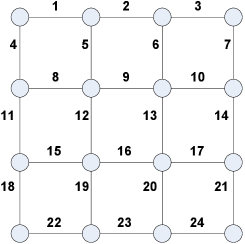
Figure 1: A 24-link grid network topology.

We first evaluate the performance of the scheduling algorithms in a grid network with 16 nodes and 24 links as shown in Fig. 1. Each node is represented by a circle and each link is illustrated by a solid line with a label indicating its index. Each link maintains its own queue. We assume $1$-hop interference.

Consider the following four sets of links:

$${\cal L}_{1}=\{1,3,8,10,15,17,22,24\},$$

$${\cal L}_{2}=\{4,5,6,7,18,19,20,21\},$$

$${\cal L}_{3}=\{1,3,9,11,14,16,22,24\},$$

$${\cal L}_{4}=\{2,4,7,12,13,18,21,23\}.$$

Each set represents a (maximum-size) maximal schedule of the network. Let $\mathbf{M}_{i}=\mathbf{e}_{{\cal L}_{i}}$, where $\mathbf{e}_{{\cal L}_{i}}$ is a vector in which the components with indices in ${\cal L}_{i}$ are $1$’s and others are $0$’s. Then, we let the arrival rate vector be a convex combination of those maximal schedules scaled by $\rho$:

$$\bm{\lambda}=\rho\cdot\sum_{i=1}^{4}c_{i}\mathbf{M}_{i},~{}\mathbf{c}=[0.2,0.3,0.2,0.3].$$

Note that a convex combination of several maximum-size maximal schedules must lie on the boundary of the capacity region. Hence the parameter $\rho$ in $[0,1]$ can be viewed as the traffic intensity, with $\rho\rightarrow 1$ representing arrival rates approaching the boundary of the capacity region.

The packet arrivals to each link $i$ follow a Bernoulli process with rate $\lambda_{i}$ independent of the packet arrival processes at other links. Each simulation experiment starts with all empty queues. For each algorithm under a fixed $\rho$, we take the average over $10$ independent experiments, with each run being $10^{5}$ time slots. Due to the high complexity of MWS in such a large network, we do not implement it here.

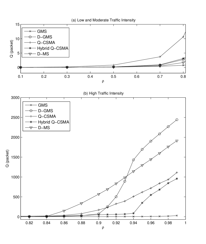
Figure 2: Long-term average queue length per link in the 24-link grid network.

For fair comparison, we choose a control overhead of $48$ mini-slots for every distributed scheduling algorithm (which lies in the range of the backoff window size specified in IEEE 802.11 DCF [3]). The parameter setting of the scheduling algorithms is summarized below.

• D-MS: $W=48$.

• D-GMS: $B=3,~{}W=16$; $b=8$.

• Q-CSMA: $W=48$; link weight $w_{i}(t)=\log(0.1q_{i}(t))$ and link activation probability $p_{i}=\frac{e^{w_{i}(t)}}{e^{w_{i}(t)}+1}$.

• Hybrid Q-CSMA: $W_{0}=5$ for the Q-CSMA procedure, $B=3$ and $W_{1}=14$ for the D-GMS procedure, plus $1$ transition mini-slot. The queue-length threshold $q_{0}=100$. Other parameters are the same as Q-CSMA.

Remark 8

In Q-CSMA we choose the link weight function $w_{i}(t)=\log(\alpha q_{i}(t))$ with a small constant $\alpha$. The rationality is to make the link weights change much slower than the dynamics of the CSMA Markov chain (to satisfy the time-scale separation assumption). We have tried several other choices for the link weight functions suggested in prior literature (such as $\alpha q_{i}(t)$ in [12] and $\log\log(q_{i}(t)+e)$ in [24]) but $\log(\alpha q_{i}(t))$ seems to give the best delay performance.

The performance of the scheduling algorithms is shown in Fig. 2, from which we can see that:

• Under low to moderate traffic intensity, D-GMS and D-MS have very good delay performance (small long-term average queue length) and perform better than Q-CSMA. However, when the traffic intensity is high, the average queue length under D-GMS/D-MS blows up and their delay performance becomes much worse than Q-CSMA.

• Hybrid Q-CSMA has the best delay performance among the distributed scheduling algorithms. It retains the stability property of Q-CSMA even under high traffic intensity while significantly reduces the delay of pure Q-CSMA. Note that when $\rho\rightarrow 1$, the performance of Hybrid Q-CSMA becomes close to pure Q-CSMA since the effect of the D-GMS procedure diminishes when the queue lengths of most links exceed the queue length threshold.

• Centralized GMS has excellent delay performance, but it is not throughput-optimal in general, as illustrated next.

We have tested the algorithms under other traffic patterns, e.g., different arrival rate vectors, Poisson arrivals, and the results are similar.

VI-B A 9-Link Ring Network

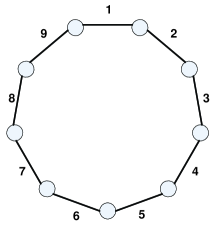
Figure 3: A 9-link ring network topology.

Consider a 9-link ring network under the $2$-hop interference model, as shown in Fig. 3. It was shown in [16] that GMS can only achieve $2/3$ of the capacity region in this network. To see this, we construct a traffic pattern using the idea in [14]. Define

$${\cal L}_{i}=\{i,(i+4)\mod 9\},\mbox{ }1\leq i\leq 9.$$

Starting with empty queues, in time slot $9k+i~{}(k\in\mathbb{Z})$, one packet arrives at each of the $2$ links in ${\cal L}_{i}$, and, with probability $\epsilon$, an additional packet arrives at each of the $9$ links. The average arrival rate vector is then $\bm{\lambda}=(\frac{2}{9}+\epsilon)\mathbf{e}$, where $\mathbf{e}$ is a vector with all components equal to $1$. It has been shown in [14] that GMS will lead to infinite queue lengths under such a traffic pattern for all $\epsilon>0$.

On the other hand, we could use a scheduling policy as follows. Define

$${\cal\tilde{L}}_{1}=\{1,4,7\},~{}{\cal\tilde{L}}_{2}=\{2,5,8\},~{}{\cal\tilde{L}}_{3}=\{3,6,9\},$$

and let $\mathbf{\tilde{M}}_{i}=\mathbf{e}_{{\cal\tilde{L}}_{i}}$ for $1\leq i\leq 3.$ In time slot $3k+i~{}(k\in\mathbb{Z})$, the maximal schedule $\mathbf{\tilde{M}}_{i}$ is used. Hence, the average service rate vector is $\bm{\mu}=\frac{1}{3}\mathbf{e}$. When $0<\epsilon<\frac{1}{9}$, $\bm{\lambda}<\bm{\mu}$, i.e., $\bm{\lambda}$ lies in the interior of the capacity region, but GMS cannot keep the network stable as we saw above.

We evaluate the performance of the scheduling algorithms under the above traffic pattern. Each simulation experiment starts with all empty queues. For each algorithm under a fixed $\epsilon$, we take the average over $10$ independent experiments, with each run being $10^{5}$ time slots. We use exactly the same parameter setting as in Section VI-A.

In Fig. 4 we can see that Q-CSMA and Hybrid Q-CSMA have a much lower delay than GMS, D-GMS (when $\epsilon\geq 0.03$) and D-MS (when $\epsilon\geq 0.05$). Fig. 5 shows that the average queue length increases linearly with the running time ($\#$ of time slots) under D-GMS/D-MS which imply that they are not stable, while the average queue length becomes stable under Q-CSMA/Hyrbid Q-CSMA.

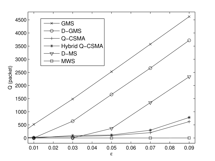
Figure 4: Long-term average queue length per link in the 9-link ring network.

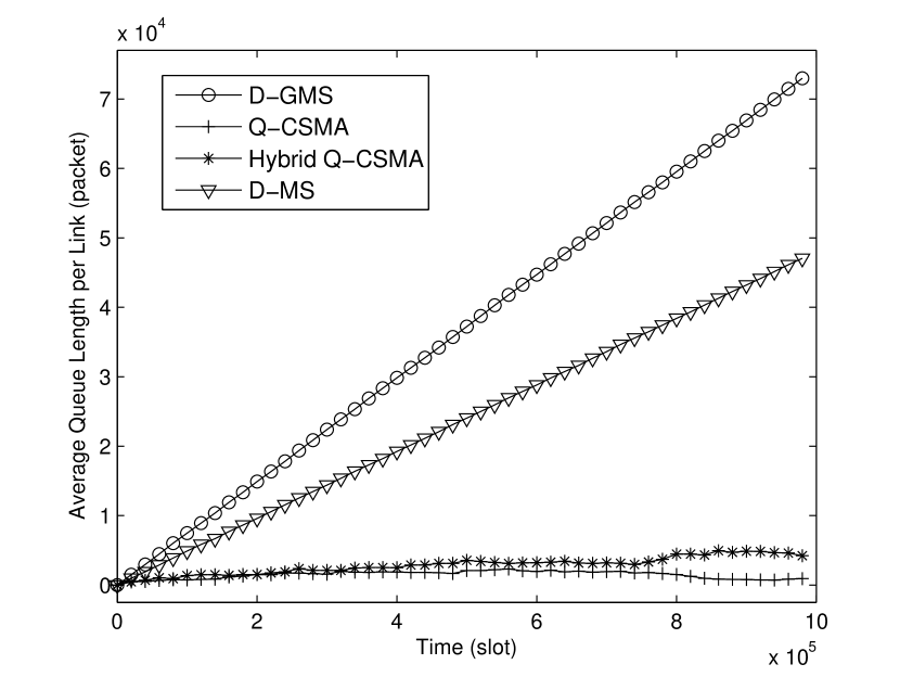
Figure 5: Sample paths of average queue length per link: $\epsilon=0.09$.

VII Conclusion

In this paper, we proposed a discrete-time distributed queue-length based CSMA/CA protocol that leads to collision-free data transmission schedules. The protocol is provably throughput-optimal. The discrete-time formulation allows us to incorporate mechanisms to dramatically reduce the delay without affecting the theoretical throughput-optimality property. In particular, combining CSMA with distributed GMS leads to very good delay performance.

We believe that it should be straightforward to extend our algorithms to be applicable to networks with multi-hop traffic and congestion-controlled sources (see [18, 10, 25] for related surveys).

-A Node-Based Implementation of Q-CSMA

For any node $n$ in the network, we use $\mathcal{N}(n)$ to denote the neighborhood of $n$, which is the set of nodes that can hear the transmission of $n$. We assume symmetry in hearing: if $n^{\prime}\in\mathcal{N}(n)$ then $n\in\mathcal{N}(n^{\prime})$.

Let $s_{i}$ and $r_{i}$ be the sender node and receiver node of link $i$, respectively. If link $i$ is included in the transmission schedule, then in the data slot, $s_{i}$ will send a data packet to $r_{i}$, and $r_{i}$ will reply an ACK packet to $s_{i}$. We assume that the data transmission from $s_{i}$ to $r_{i}$ is successful if no nodes in $\mathcal{N}(r_{i})$ are transmitting in the same time; similarly, the ACK transmission from $r_{i}$ to $s_{i}$ is successful if no nodes in $\mathcal{N}(s_{i})$ are transmitting in the same time. We also consider the node-exclusive constraint that two active links cannot share a common node. Therefore, in a synchronized data/ACK transmission system, the conflict set of link $i$ is:

$$\mathcal{C}(i) = \Big{\{}j:j\mbox{ shares a common node with }i,$$

$$\mbox{ or }s_{j}\in\mathcal{N}(r_{i}),\mbox{ or }r_{j}\in\mathcal{N}(s_{i}).\Big{\}}.$$

In summary, two links $i$ and $j$ conflict with each other, i.e., $i\in\mathcal{C}(j)$ and $j\in\mathcal{C}(i)$, if they share a common node, or if simultaneous data transmissions at $s_{i}$ and $s_{j}$ will collide at $r_{i}$ and $r_{j}$, or if simultaneous ACK transmissions at $r_{i}$ and $r_{j}$ will collide at $s_{i}$ and $s_{j}$.

We say that a node is active in a time slot if it is the sender node or receiver node of an active link. In a time slot, each inactive node will conduct carrier sensing. It will determine whether there are some active sender nodes and some active receiver nodes in its neighborhood by sensing whether the channel is busy during the data transmission period and during the ACK transmission period, respectively. In this way, link $i$ “knows” that no links in its conflict set are active in a time slot, if $s_{i}$ and $r_{i}$ don’t belong to an active link other than $i$, $s_{i}$ does not sense an active receiver node in $\mathcal{N}(s_{i})$, and $r_{i}$ does not sense an active sender node in $\mathcal{N}(r_{i})$.

Similar to the RTS/CTS mechanism in the 802.11 MAC protocol, an INTENT message “sent” by a link consists of an RTD (Request-To-Decide) and a CTD (Clear-To-Decide) pair exchanged by the sender node and receiver node of the link. To achieve this, we further divide a control mini-slot into two sub-mini-slots. In the first sub-mini-slot, $s_{i}$ sends an RTD to $r_{i}$. If $r_{i}$ receives the RTD without a collision (i.e., no nodes in $\mathcal{N}(r_{i})$ are transmitting in the same sub-mini-slot), then $r_{i}$ will reply a CTD to $s_{i}$ in the second sub-mini-slot. If $s_{i}$ receives the CTD from $r_{i}$ without a collision, then link $i=(s_{i},r_{i})$ will be added to the decision schedule. We choose the length of a sub-mini-slot such that an RTD or CTD sent by any node can reach its neighbors within one sub-mini-slot. Note that the exchange of an RTD/CTD pair between the sender and receiver of a link will “silence” all its conflicting links so those links will not be added to the decision schedule anymore.

Now we are ready to present the node-based Q-CSMA algorithm. Some additional one-bit memories maintained at node $n$ (in time slot $t$) are summarized below (each explanation corresponds to bit $1$):

• $A\!S_{n}(t)/A\!R_{n}(t)$: $n$ is available as the sender/receiver node for a link in the decision schedule $\mathbf{m}(t)$.

• $A\!C\!T_{n}(t)$: $n$ is active (as either a sender or receiver node).

• $N\!S_{n}(t)/N\!R_{n}(t)$: the neighborhood of $n$ (i.e, ${\cal N}(n)$) has an active sender/receiver node.

Q-CSMA Algorithm (at Node $n$ in Time Slot $t$)

• At the beginning of the time slot, node $n$ sets $A\!S_{n}(t)=1$ and $A\!R_{n}(t)=1$.
  Let $L(n)$ be the set of links for which $n$ is the sender node (i.e., $n=s_{l}$, $\forall l\in L(n)$). Node $n$ randomly chooses one link in $L(n)$ (suppose link $i=(n,m)$ is chosen) and selects a backoff time $T_{i}$ uniformly in $[0,W-1]$. Other links in $L(n)$ will not be included in $\mathbf{m}(t)$, so $x_{l}(t)=x_{l}(t-1),\forall l\in L(n)\setminus i$.

• Throughout the control slot, if node $n$ senses an RTD transmission not intended for itself (or a collision of RTDs) by a node in $\mathcal{N}(n)$, $n$ will no longer be available as the receiver node for a link in $\mathbf{m}(t)$. Thus, node $n$ will set $A\!R_{n}(t)=0$.

• Before the $(T_{i}+1)$-th control mini-slot, if node $n$ senses a CTD transmission by a node in $\mathcal{N}(n)$ (or a collision of CTDs), $n$ will no longer be available as the sender node for a link in $\mathbf{m}(t)$, and it will set $A\!S_{n}(t)=0$. In this case link $i$ will not be included in $\mathbf{m}(t)$ and $x_{i}(t)=x_{i}(t-1)$.

• At the beginning of the $(T_{i}+1)$-th control mini-slot, if $A\!S_{n}(t)=1$, node $n$ will send an RTD to node $m$ in the first sub-mini-slot. Node $n$ will then set $A\!S_{n}(t)=A\!R_{n}(t)=0$.

  • If node $m$ receives the RTD from node $n$ without a collision and $A\!R_{m}(t)=1$, $m$ will send a CTD to $n$ in the second sub-mini-slot of the $(T_{i}+1)$-th control mini-slot. Node $m$ will then set $A\!S_{m}(t)=A\!R_{m}(t)=0$. The CTD message also includes the carrier sensing information of node $m$ in the previous time slot (the values of $A\!C\!T_{m}(t-1)$ and $N\!S_{m}(t-1)$). Otherwise, no message will be sent.

  • If node $n$ receives the CTD message from node $m$ without a collision, link $i=(n,m)$ will be included in $\mathbf{m}(t)$. Node $n$ will decide link $i$’s state as follows:
    aaa if no links in $\mathcal{C}(i)$ were active in the previous data slot, i.e., $x_{i}(t-1)=1$ or $A\!C\!T_{n}(t-1)=A\!C\!T_{m}(t-1)=N\!R_{n}(t-1)=N\!S_{m}(t-1)=0$
    aaaaaa $x_{i}(t)=1$ with probability $p_{i}$, $0<p_{i}<1$;
    aaaaaa $x_{i}(t)=0$ with probability $\bar{p}_{i}=1-p_{i}$.
    aaa else
    aaaaaa $x_{i}(t)=0$.
    Otherwise, link $i$ will not be included in $\mathbf{m}(t)$ and $x_{i}(t)=x_{i}(t-1)$.

• In the data slot, node $n$ takes one of the three different roles:

  • Sender: $x_{l}(t)=1$ for some link $l=(n,m)\in E$. Node $n$ will send a data packet to node $m$ and set $A\!C\!T_{n}(t)=1$.

  • Receiver: $x_{l}(t)=1$ for some link $l=(m,n)\in E$. Node $n$ will send an ACK packet to node $m$ (after it receives the data packet from $m$) and set $A\!C\!T_{n}(t)=1$.

  • Inactive: Node $n$ sets $A\!C\!T_{n}(t)=0$ and conducts carrier sensing. Recall that data/ACK transmissions in our system are synchronized. Thus, node $n$ will set $N\!S_{n}(t)=0$ if it senses no signal during the data transmission period and set $N\!S_{n}(t)=1$ otherwise. Similarly, node $n$ will set $N\!R_{n}(t)=0$ if it senses no signal during the ACK transmission period and set $N\!R_{n}(t)=1$ otherwise.

Remark 9

Note that RTD and CTD are sent in two different sub-mini-slots. This provides an easy way to differentiate RTD and CTD (or collisions of RTDs and CTDs, respectively) without having to encode the packet type in a preamble bit of such a control packet (actually when a collision happens, a node cannot even check this “packet type” bit to differentiate RTD and CTD).

Proposition 6

$\mathbf{m}(t)$ produced by the node-based Q-CSMA algorithm is a feasible schedule. Let $\mathcal{M}_{0}$ be the set of decision schedules produced by the algorithm. If the window size $W\geq 2$, then $\cup_{\mathbf{m}\in\mathcal{M}_{0}}\mathbf{m}=E$ and the algorithm achieves the product-form distribution in Proposition 1.

Proof:

The proof is similar to the proof of Lemma 3. Under the node-based Q-CSMA algorithm, link $i$ will be included in the decision schedule $\mathbf{m}(t)$ if and only if its sender and receiver nodes successfully exchange an RTD/CTD pair in the control slot. This will “silence” all the receivers in $\mathcal{N}(s_{i})$ and all the senders in in $\mathcal{N}(r_{i})$ as well as nodes $s_{i}$ and $r_{i}$, so no links in $\mathcal{C}(i)$ will be included in $\mathbf{m}(t)$. Hence $\mathbf{m}(t)$ is a feasible schedule. Similarly, for any maximal schedule $\mathbf{m}$, we can check that $\mathbf{m}$ will be selected in the control slot with positive probability if the window size $W\geq 2$. Since the set of all maximal schedules will include all links, $\cup_{\mathbf{m}\in\mathcal{M}_{0}}\mathbf{m}=E$. Then by Proposition 1 the node-based Q-CSMA algorithm achieves the product-form distribution. ∎

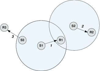
Figure 6: Hidden and Exposed Terminal Problems

-B Elimination of Hidden and Exposed Terminal Problems

In IEEE 802.11 DCF, the RTS/CTS mechanism is used to reduce the Hidden Terminal Problem. However, even if RTS/CTS is used, the hidden terminal problem can still occur, as illustrated in Fig. 6, where we use $S_{i}$ and $R_{i}$ to denote the sender and receiver (in the sense of data transmission) of link $i$. Under 802.11, it is possible that $S_{2}$ is sending an RTS to $R_{2}$ while $R_{1}$ is returning a CTS to $S_{1}$ at the same time. $R_{1}$ cannot detect the RTS from $S_{2}$ since it is transmitting. Likewise, $S_{2}$ cannot detect the CTS from $R_{2}$. Therefore, both links 1 and 2 could be scheduled, which causes a collision at $R_{1}$.

Our Q-CSMA algorithm, however, can resolve the hidden terminal problem because the RTD/CTD messages are exchanged in a synchronized manner. Suppose $T_{i}$ is the backoff expiration time of node $S_{i}$.

• $T_{1}<T_{2}$: During the $(T_{1}+1)$-th mini-slot, $S_{1}$ sends an RTD in the first sub-mini-slot, then in the second sub-mini-slot, $R_{1}$ returns a CTD, and link $1$ will be included in the decision schedule. Since this CTD is not intended for $S_{2}$, $S_{2}$ disables its role as a sender of a link in the decision schedule, thus link $2$ will not be included in the decision schedule.

• $T_{1}=T_{2}$: During the $(T_{1}+1)$-th mini-slot , both $S_{1}$ and $S_{2}$ send an RTD in the first sub-mini-slot. In this case, $R_{1}$ senses a collision of RTD and will not return a CTD. Thus, link $1$ will not be included in the decision schedule, while link $2$ will be included in the decision schedule.

• $T_{1}>T_{2}$: Similarly, in this case link $2$ but not link $1$ will be included in the decision schedule.

Therefore, under synchronized RTD/CTD, the decision schedule is collision-free, which implies that the transmission schedule is collision-free if we start with a collision-free transmission schedule (e.g., the empty schedule), see Lemma 1. Hence the hidden terminal problem is eliminated.

Another problem, known as the Exposed Terminal Problem, may also occurs under 802.11. In Fig. 6, if $S_{1}$ sends an RTS to $R_{1}$, $S_{3}$ will receive this RTS and will be silenced under 802.11, which is unnecessary because the potential transmission of link $3$ will not interfere with link $1$. On the other hand, under Q-CSMA, if $S_{1}$ sends an RTD to $R_{1}$, $S_{3}$ will ignore this RTD and can still send an RTD to $R_{3}$. Therefore, both links $1$ and $3$ can be included in the decision schedule and in the transmission schedule, thus avoiding the exposed terminal problem.

Note that the presence of hidden and exposed terminals not only leads to loss of efficiency, but also poses mathematical difficulties. For example, when there are hidden and exposed terminals in an 802.11-type asynchronous RTS/CTS model, it is impossible to define a set of schedules that are consistent with both the definition of a feasible schedule as defined in (1) and the capacity region as defined in (2). Our RTD/CTD mechanism eliminates such problems.

References

- [1] U. Akyol, M. Andrews, P. Gupta, J. Hobby, I. Saniee, and A. Stolyar. Joint scheduling and congestion control in mobile ad-hoc networks. In Proceedings of IEEE INFOCOM, April 2008.
- [2] V. Bharghavan, A. Demers, S. Shenker, and L. Zhang. MACAW: a media access protocol for wireless LAN’s. In Proceedings of ACM SIGCOMM, 1994.
- [3] G. Bianchi. Performance analysis of the IEEE 802.11 distributed coordination function. IEEE Journal on Selected Areas in Communications, 18(3):535–547, 2000.
- [4] R. R. Boorstyn, A. Kershenbaum, B. Maglaris, and V. Sahin. Throughput analysis in multihop CSMA packet radio networks. IEEE Transactions on Communications, 35(3):267–274, March 1987.
- [5] C. Bordenave, D. McDonald, and A. Proutiere. Performance of random multi-access algorithms, an asymptotic approach. In Proceedings of ACM Sigmetrics, June 2008.
- [6] P. Chaporkar, K. Kar, and S. Sarkar. Throughput guarantees through maximal scheduling in wireless networks. In Proceedings of 43rd Annual Allerton Conference on Communication, Control and Computing, 2005.
- [7] A. Dimakis and J. Walrand. Sufficient conditions for stability of longest-queue-first scheduling: Second-order properties using fluid limits. Advances in Applied Probabilities, 38(2):505–521, 2006.
- [8] M. Durvy and P. Thiran. Packing approach to compare slotted and non-slotted medium access control. In Proceedings of IEEE INFOCOM, April 2006.
- [9] A. Eryilmaz, R. Srikant, and J. R. Perkins. Stable scheduling policies for fading wireless channels. IEEE/ACM Transactions on Networking, 13(2):411–424, April 2005.
- [10] L. Georgiadis, M. Neely, and L. Tassiulas. Resource allocation and cross-layer control in wireless networks. Foundations and Trends in Networking, 2006.
- [11] L. Jiang and J. Walrand. Convergence analysis of a distributed CSMA algorithm for maximal throughput in a general class of networks. Technical Report, UC Berkeley, December 2008.
- [12] L. Jiang and J. Walrand. A distributed CSMA algorithm for throughput and utility maximization in wireless networks. In Proceedings 46th Annual Allerton Conference on Communication, Control and Computing, September 2008.
- [13] L. Jiang and J. Walrand. Approaching throughput-optimality in a distributed CSMA algorithm with contention resolution. Technical Report, UC Berkeley, March 2009.
- [14] C. Joo, X. Lin, and N. B. Shroff. Understanding the capacity region of the greedy maximal scheduling algorithm in multi-hop wireless networks. In Proceedings of IEEE INFOCOM, April 2008.
- [15] F. Kelly. Reversibility and Stochastic Networks. Wiley, Chichester, 1979.
- [16] M. Leconte, J. Ni, and R. Srikant. Improved bounds on the throughput efficiency of greedy maximal scheduling in wireless networks. In Proceedings of ACM MOBIHOC, May 2009.
- [17] S. C. Liew, C. Kai, J. Leung, and B. Wong. Back-of-the-envelope computation of throughput distributions in CSMA wireless networks. Submitted for publication, http://arxiv.org//pdf/0712.1854.
- [18] X. Lin, N. B. Shroff, and R. Srikant. A tutorial on cross-layer optimization in wireless networks. IEEE Journal on Selected Areas in Communications, 2006.
- [19] J. Liu, Y. Yi, A. Proutiere, M. Chiang, and H. V. Poor. Maximizing utility via random access without message passing. Microsoft Research Technical Report, September 2008.
- [20] P. Marbach, A. Eryilmaz, and A. Ozdaglar. Achievable rate region of CSMA schedulers in wireless networks with primary interference constraints. In Proceedings of IEEE CDC, December 2007.
- [21] F. Martinelli. Lectures on Glauber dynamics for discrete spin models. Lectures on probability theory and statistics (Saint-Flour, 1997), Lecture Notes in Math., 1717, Springer, Berlin, 1999.
- [22] A. Proutiere, Y. Yi, and M. Chiang. Throughput of random access without message passing. In Proceedings of CISS, March 2008.
- [23] S. Rajagopalan and D. Shah. Distributed algorithm and reversible network. In Proceedings of CISS, March 2008.
- [24] S. Rajagopalan, D. Shah, and J. Shin. Aloha that works, November 2008. Submitted.
- [25] S. Shakkottai and R. Srikant. Network optimization and control. Foundations and Trends in Networking, pages 271–379, 2007.
- [26] L. Tassiulas and A. Ephremides. Stability properties of constrained queueing systems and scheduling policies for maximal throughput in multihop radio networks. IEEE Transactions on Automatic Control, 37(12):1936–1948, December 1992.
- [27] X. Wang and K. Kar. Throughput modelling and fairness issues in CSMA/CA based ad-hoc networks. In Proceedings of IEEE INFOCOM, March 2005.
- [28] A. Warrier, S. Janakiraman, and I. Rhee. DiffQ: Practical differential backlog congestion control for wireless networks. In Proceedings of IEEE INFOCOM, 2009.
- [29] X. Wu, R. Srikant, and J. R. Perkins. Queue-length stability of maximal greedy schedules in wireless networks. IEEE Transactions on Mobile Computing, pages 595–605, June 2007.
- [30] G. Zussman, A. Brzezinski, and E. Modiano. Multihop local pooling for distributed throughput maximization in wireless networks. In Proceedings of IEEE INFOCOM, April 2008.