Derivation and study of dynamical models
of dislocation densities

Abstract

In this paper, starting from the microscopic dynamics of isolated dislocations, we explain how to derive formally mean field models for the dynamics of dislocation densities. Essentially these models are tranport equations, coupled with the equations of elasticity. Rigorous results of existence of solutions are presented for some of these models and the main ideas of the proofs are given.

AMS Classification: 54C70, 35L45, 35Q72, 74H20, 74H25. Key words: Cauchy’s problem, non-linear transport equations, non-local transport equations, hyperbolic equations, BMO estimate, dynamics of dislocation densities.

Introduction

In this paper we are interested in several mesoscopic models involving the dynamics of dislocations. These models are important for the understanding of the elasto-visco-plasticity behaviour of materials. For crystals, at the microscopic level, the origin of plasticity is mainly due to the existence of defects called dislocations. Dislocations are line defects that can move in the crystal when a shear stress is applied. On the other hand each dislocation also creates a stress field. This leads to a complicated dynamics of these defects that we consider below. See Figure 1 for an example of complicated pattern of dislocations in real crystals.

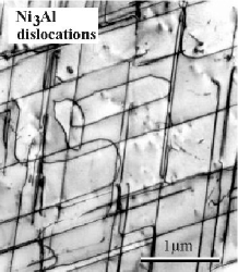
Figure 1: Dislocation lines in Nickel Aluminium alloy.

Organization of the paper.
Section 1 presents the microscopic modelling for the dynamics of dislocation straight lines. In Section 2, we explain how to derive formally a two-dimensional mean field model, called the Groma, Balogh model. A rigorous result of existence of solutions is given and other results are also given for a one-dimenional submodel. In Section 3, the Groma, Czikor, Zaiser model is studied. In particular is presented a simulation of the deformation of a slab under an external shear stress. In Section 4, the formal derivation of a mean field model for densities of dislocation curves is presented. Concluding remarks are given in Section 5.

1 The microscopic modelling

1.1 Preliminary: the stress field created by an edge dislocation

In the space coordinates $x=(x_{1},x_{2},x_{3})$ with basis $(e_{1},e_{2},e_{3})$, we consider the case a material filling the whole space and with a single dislocation line which is the axis $x_{3}$. To this line is associated an invariant, called the Burgers vector $b$. In the case of linear isotropic elasticity with Lamé coefficients $\lambda,\mu$ (satisfying $\mu>0,3\lambda+2\mu>0$), the stress created by the dislocation is given by

$$\sigma_{ij}=2\mu e_{ij}+\lambda\left(\sum_{k=1,2,3}e_{kk}\right)\delta_{ij},\quad i,j=1,2,3$$ (1.1)

where

$$e_{ij}=\frac{1}{2}\left(\frac{\partial u_{j}}{\partial x_{i}}+\frac{\partial u_{i}}{\partial x_{j}}\right)+H(x_{1})\delta_{0}(x_{2})e^{0}_{ij}\quad\mbox{with}\quad e^{0}=\frac{1}{2}\left(b\otimes n+n\otimes b\right)$$

where $H$ is the Heaviside function, $\delta_{0}$ is the Dirac mass, $n=e_{2}$ is the normal to the slip plane and $(u_{1},u_{2},u_{3})$ is the three-dimensional displacement field. In the special case where $b=e_{1}$, the dislocation is called an edge dislocation (the Burgers vector is perpendicular to the dislocation line). In this case we have

$$e^{0}=\frac{1}{2}\left(\begin{array}[]{lll}0&1&0\\ 1&0&0\\ 0&0&0\end{array}\right).$$ (1.2)

The stress is assumed to satisfy the elasticity equation of equilibrium

$$\sum_{i=1,2,3}\frac{\partial\sigma_{ij}}{\partial x_{i}}=0,\quad j=1,2,3.$$ (1.3)

The solution to this equation is known since the work of Volterra [16]. We have (see Hirth, Lothe [7]):

$$\sigma(x)=a\left(\begin{array}[]{ccc}\displaystyle{-\frac{x_{2}(3x_{1}^{2}+x_{2}^{2})}{(x_{1}^{2}+x_{2}^{2})^{2}}}&\displaystyle{\frac{x_{1}(x_{1}^{2}-x_{2}^{2})}{(x_{1}^{2}+x_{2}^{2})^{2}}}&0\\ \\ \displaystyle{\frac{x_{1}(x_{1}^{2}-x_{2}^{2})}{(x_{1}^{2}+x_{2}^{2})^{2}}}&\displaystyle{\frac{x_{2}(x_{1}^{2}-x_{2}^{2})}{(x_{1}^{2}+x_{2}^{2})^{2}}}&0\\ \\ 0&0&0\end{array}\right)$$ (1.4)

with

$$a=\frac{\mu}{2\pi(1-\nu)}>0\quad\mbox{where the Poisson ratio is}\quad\displaystyle{\nu=\frac{\lambda}{2(\lambda+\mu)}\in\left(-1,\frac{1}{2}\right)}.$$

1.2 A two-dimensional microscopic model

In this section we describe very formally a microscopic model describing the dynamics of dislocation lines in the particular geometry where all lines are parallel to the axis $x_{3}$.

Considering the cross section of these lines, we can reduce the problem to a two-dimensional problem where each dislocation line can be identified to its position $(x_{1},x_{2})$. For $i=1,...,N$, let us call $X^{i}$ the positions in ${\mathbb{R}}^{2}$ of these dislocations (see Figure 2).

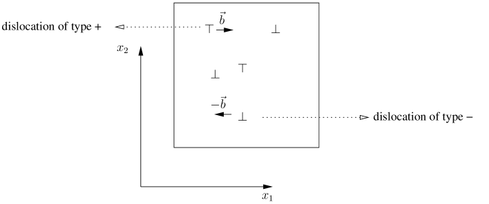
Figure 2: The cross section of the dislocation lines.

We consider moreover the particular case where each dislocation can only move along the direction $e_{1}$. Those dislocations $X^{i}$ are known to be characterized by an invariant called the Burgers vector $b_{i}=\varepsilon_{i}e_{1}$ where

$$\varepsilon_{i}=\pm 1.$$

Finally the dynamics of these dislocations is

$$\frac{dX^{i}(t)}{dt}=b_{i}\ \sigma_{12}(X^{i}(t)),\quad\mbox{for}\quad i=1,...,N.$$ (1.5)

Here $\sigma_{12}$ is one component of the stress. In the case of linear isotropic elasticity, it is known that

$$\sigma_{12}(x)=\sum_{i=1,...,N}\varepsilon_{i}\sigma_{0}(x-X^{i}),\quad\mbox{where}\quad\sigma_{0}(x)=a\ \displaystyle{\frac{x_{1}(x_{1}^{2}-x_{2}^{2})}{(x_{1}^{2}+x_{2}^{2})^{2}}},$$

where $\sigma_{0}$ is the $(1-2)$-component of the stress given in (1.4). Here $\sigma_{0}(x)$ appears to be the shear stress created at the point $x$ by a single dislocation positionned at the origin, with Burgers vector $e_{1}$. With the convention that the self-stress created by a dislocation on itself is zero, i.e. formally $\sigma_{0}(0)=0$, we see that we can rewrite the full dynamics of particles satisfying $X^{i}\not=X^{j}$ for $i\not=j$, as follows

$$\frac{dX^{i}}{dt}=e_{1}\ \left(\sum_{j\in\left\{1,...,N\right\}\backslash\left\{i\right\}}\varepsilon_{i}\varepsilon_{j}\sigma_{0}(X^{i}-X^{j})\right),\quad\mbox{for}\quad i=1,...,N.$$

Let us now introduce the “density” of dislocations

$$\theta^{\pm}(x,t)=\sum_{i\in\left\{1,...,N\right\}\ :\ \varepsilon_{i}=\pm 1}\delta_{0}(x-X^{i}(t))$$

where $\theta^{+}$ and $\theta^{-}$ correspond respectively to the dislocations with positive and negative Burgers vector. Again with the convention $\sigma_{0}(0)=0$, we can rewrite the dynamics as

$$\theta^{\pm}_{t}+\mbox{div}\ \left(\pm J\ \theta^{\pm}\right)=0\quad\mbox{with}\quad J=e_{1}\ \sigma_{0}\star(\theta^{+}-\theta^{-}).$$ (1.6)

2 Mesoscopic models

2.1 Formal derivation of the two-dimensional mesoscopic model

A natural question is what is the effective model at the mesocsopic scale corresponding to the microscopic model (1.6)? It seems to be an open and difficult question. As a naive answer, we can consider as a first candidate to the mesoscopic model, the mean field model corresponding to the model (1.6), where now each density $\theta^{+}$ and $\theta^{-}$ can be seen as a “continuous” quantity. In this mean field model, we have in particular neglected the short range dynamics. One convenient way to rewrite the model is to introduce one primitive $\rho^{\pm}$ of the densities $\theta^{\pm}$ such that

$$\rho^{\pm}_{x_{1}}(x,t)=\theta^{\pm}(x,t)\geq 0.$$

Then we can rewrite (1.6) as (with a zero constant of integration):

$$\rho^{\pm}_{t}=\mp\sigma_{12}\ \rho^{\pm}_{x_{1}}$$ (2.7)

with

$$\sigma_{12}=(\sigma_{0})_{x_{1}}\star(\rho^{+}-\rho^{-}).$$ (2.8)

System (2.7)-(2.8) is an integrated form of the Groma, Balogh model (1.6) (see [5]). It turns out that by construction $\sigma$ solves:

$$\left\{\begin{array}[]{l}\displaystyle{\sum_{i=1,2,3}\frac{\partial\sigma_{ij}}{\partial x_{i}}=0},\\ \displaystyle{\sigma_{ij}=2\mu e_{ij}+\lambda\left(\sum_{k=1,2,3}e_{kk}\right)\delta_{ij}},\\ \displaystyle{e_{ij}=\frac{1}{2}\left(\frac{\partial u_{j}}{\partial x_{i}}+\frac{\partial u_{i}}{\partial x_{j}}\right)+(\rho^{+}-\rho^{-})e^{0}_{ij}},\end{array}\right.$$ (2.9)

where $e^{0}$ is given in (1.2). Here (2.8) appears to be a representation formula for the solution of the equations of elasticity (2.9).

2.2 Existence of a solution in the two-dimensional periodic case

In the case where the dislocations densities $\theta^{\pm}(x,t)$ are ${\mathbb{Z}}^{2}$-periodic in $x\in{\mathbb{R}}^{2}$ such that

$$\int_{0}^{1}dx_{1}\ \theta^{\pm}(x_{1},x_{2},t)=L>0,$$

it turns out that the representation formula (2.8) can be rewritten

$$\sigma_{12}=\bar{a}\ R_{1}^{2}R_{2}^{2}(\rho^{+}-\rho^{-})\quad\mbox{with}\quad\bar{a}=4\mu(\lambda+\mu)/(\lambda+2\mu),$$ (2.10)

where $R_{i}$ for $i=1,2$ are the Riesz transform given in Fourier series coefficients on $\mathbb{T}^{2}={\mathbb{R}}^{2}/{\mathbb{Z}}^{2}$ by

$$c_{k}(R_{i}(f))=\left\{\begin{array}[]{ll}\displaystyle{\frac{k_{i}}{|k|}c_{k}(f)}&\quad\mbox{for all}\quad k=(k_{1},k_{2})\in{\mathbb{Z}}^{2}\backslash\left\{(0,0)\right\}\\ 0&\quad\mbox{if}\quad k=(0,0)\end{array}\right.$$

where

$$c_{k}(f)=\int_{\mathbb{T}^{2}}e^{-2i\pi k\cdot x}f(x)\ d^{2}x.$$

We will also make use of the norm on the following Zygmund space

$$||f||_{L\ln L(\mathbb{T}^{2})}=\inf\left\{\gamma>0,\quad\int_{\mathbb{T}^{2}}\frac{|f|}{\gamma}\ln\left(e+\frac{|f|}{\gamma}\right)\leq 1\right\}.$$

We assume that

$$\rho^{\pm}(\cdot,0)=\rho^{\pm}_{0}$$ (2.11)

and we make the following assumptions on the initial data

$$\left\{\begin{array}[]{l}\rho^{\pm}_{0}(x_{1}+m,x_{2}+l)=mL+\rho^{\pm}_{0}(x_{1},x_{2})\quad\mbox{for any}\quad m,l\in{\mathbb{Z}}\\ \\ (\rho^{\pm}_{0})_{x_{1}}\geq 0\\ \\ ||(\rho^{\pm}_{0})_{x_{1}}||_{L\ln L(\mathbb{T}^{2})}\leq C\end{array}\right.$$ (2.12)

where $C>0$ is any fixed constant.

Then we have:

Theorem 2.1

(Global existence of a solution in the periodic case, [2])
Under assumption (2.12) there exists a function $(\rho^{+},\rho^{-})$ which is a solution of (2.7), (2.10) in the sense of distributions and with initial condition (2.12), such that $\rho^{\pm}(\cdot,t)$ satisfies (2.12) for all time. Moreover $\rho^{\pm}\in C([0,+\infty);L^{1}_{loc}({\mathbb{R}}^{2}))$ and

$$\sigma_{12}\in L^{2}_{loc}([0,+\infty);H^{1}_{loc}({\mathbb{R}}^{2})).$$ (2.13)

Remark 2.2

Recall that there exists a constant $C>0$ such that the general inequality holds for functions $f\in H^{1}(\mathbb{T}^{2})$ and $g\in L\ln L(\mathbb{T}^{2})$

$$||fg||_{L^{1}(\mathbb{T}^{2})}\leq C||f||_{H^{1}(\mathbb{T}^{2})}||g||_{L\ln L(\mathbb{T}^{2})}.$$

Then the product $\sigma_{12}\cdot(\rho^{\pm})_{x_{1}}$ in (2.7) is defined because of both estimate (2.13) on $\sigma_{12}$ and estimate $L^{\infty}([0,+\infty);L\ln L(\mathbb{T}^{2}))$ on $(\rho^{\pm})_{x_{1}}$.

Indeed, in the proof of Theorem 2.1, the main tool is to consider the entropy

$$S(t)=\sum_{\pm}\int_{\mathbb{T}^{2}}\theta^{\pm}(\cdot,t)\ln\theta^{\pm}(\cdot,t)\quad\mbox{with}\quad\theta^{\pm}=(\rho^{\pm})_{x_{1}}$$

which satisfies formally the following a priori estimate

$$S(t)+\bar{a}\int_{0}^{t}\int_{\mathbb{T}^{2}}(R_{1}R_{2}(\theta^{+}-\theta^{-}))^{2}\leq S(0).$$

The uniqueness of the solution remains an open problem.

2.3 A one-dimensional mesoscopic submodel

In this section, we present a submodel where the uniqueness of the solution is known.

Let us now consider a solution $(\rho^{+},\rho^{-})$ of (2.7), (2.10) only depending on the variable $y=x_{1}+x_{2}$ and on the time $t$ (see Figure 3).

Figure 3: A $1$-D sub-model invariant by translation in the $(-1,1)$ direction.

In that case, we can rewrite the system of equations for $(\rho^{+}(y,t),\rho^{-}(y,t))$ as follows:

$$\left\{\begin{array}[]{l}\displaystyle{\rho^{+}_{t}=-c_{1}\left\{(\rho^{+}-\rho^{-})+c_{2}\int_{0}^{1}dz\ (\rho^{+}(z,t)-\rho^{-}(z,t))\right\}\ \rho^{+}_{y}}\\ \\ \displaystyle{\rho^{-}_{t}=c_{1}\left\{(\rho^{+}-\rho^{-})+c_{2}\int_{0}^{1}dz\ (\rho^{+}(z,t)-\rho^{-}(z,t))\right\}\ \rho^{-}_{y}}\\ \end{array}\right.$$ (2.14)

with the constants

$$c_{1}=\frac{\mu(\lambda+\mu)}{\lambda+2\mu}>0,\quad c_{2}=\frac{\mu}{\lambda+\mu}>0.$$

For $\rho^{\pm}_{y}\geq 0$, this system looks very much like the Burgers equation in the rarefaction case (where no shocks are created). For this system, the following uniqueness result is available:

Theorem 2.3

(Uniqueness for the one-dimensional submodel, [4])
Assume that the initial data $\rho^{\pm}_{0}$ is Lipschitz non-decreasing and that for some $L>0$, the functions $y\mapsto\rho^{\pm}_{0}(y)-Ly$ are $1-periodic$. Then there exists a unique viscosity solution $(\rho^{+},\rho^{-})$ to the system (2.14),(2.11). Moreover this solution is globally Lipschitz in space and time.

In this theorem the notion of viscosity solution is the one introduced by Ishii, Koike [12] for systems which are quasi-monotone. Roughly speaking, this is related to the fact that for $c_{2}=0$, this system has a comparison principle. More precisely, if $\rho^{\pm,1}$ and $\rho^{\pm,2}$ are two solutions of system (2.14) with $c_{2}=0$ such that

$$\rho^{+,1}(y,t)\leq\rho^{+,2}(y,t)\quad\mbox{and}\quad\rho^{-,1}(y,t)\leq\rho^{-,2}(y,t)\quad\mbox{for all}\quad y\in{\mathbb{R}}$$

holds at time $t=0$, then this is true for all time $t>0$.

Moreover for system (2.14), it is possible to write an upwind scheme and to prove a Crandall-Lions type discrete-continuous error estimate for this scheme, as it is done in El Hajj, Forcadel [4].

Let us mention that an existence and uniqueness result for system (2.14) has also been obtained by El Hajj [3] in the framework of $H^{1}_{loc}({\mathbb{R}})$ initial data with solutions in $H^{1}_{loc}({\mathbb{R}}\times[0,+\infty))$.

This system has also been studied in the case of periodic external applied stress. In the system (2.14), this corresponds to add a time-periodic term to the quantity $(\rho^{+}-\rho^{-})$. Then for this non-local system, it is shown formally in Briani, Cardaliaguet, Monneau [1] (see also Souganidis, Monneau [15] for a local system in the stationary ergodic setting) that the long time behaviour of the system is an equivalent quasilinear diffusion equation.

3 The GCZ one-dimensional mesoscopic model

3.1 Presentation of the model

In this section we consider the case where the three-dimensional material is a slab $\Omega=(-1,1)\times{\mathbb{R}}^{2}$ with boundary conditions

$$\sigma\cdot n=\pm\tau e_{2}\quad\mbox{for}\quad x_{1}=\pm 1$$ (3.15)

where $\tau\in{\mathbb{R}}$ is a fixed constant (see Figure 4).

Figure 4: Geometry of the slab.

In that case, we can check that the solution to the equation (2.9) on $\Omega$ supplemented with boundary conditions (3.15), is

$$\sigma_{12}=\tau\quad\mbox{and}\quad\sigma_{ij}=0\quad\mbox{if}\quad\left\{i,j\right\}\not=\left\{1,2\right\}.$$

And then from the evolution equation (2.7), we see that in the case $\tau>0$, the positive dislocations move to the right and the negative dislocations move to the left. In order to take into account the short range dynamics with accumulations of dislocations on the boundary of the material, Groma, Czikor and Zaiser [6] have proposed to modify equation (2.7) into the following equation (GCZ model)

$$\rho^{\pm}_{t}=\mp\tilde{\sigma}_{12}\rho^{\pm}_{x_{1}}\quad\mbox{with}\quad\tilde{\sigma}_{12}={\sigma}_{12}+\tau_{b}$$ (3.16)

where $\tau_{b}$ is the back stress created by the concentration of dislocations

$$\tau_{b}=-D_{0}\ \frac{(\theta^{+}-\theta^{-})_{x_{1}}}{\theta^{+}+\theta^{-}}\quad\mbox{with}\quad\theta^{\pm}=\rho^{\pm}_{x_{1}}$$

where $D_{0}$ is a diffusion coefficient that we take equal to $1$ to simplify the presentation. Introducing the quantities

$$\rho=\rho^{+}-\rho^{-}\quad\mbox{and}\quad\kappa=\rho^{+}+\rho^{-},$$

the full GCZ system can be rewritten with $y=x_{1}\in I=(-1,1)$ as

$$\left\{\begin{array}[]{l}\rho_{t}=\rho_{yy}-\tau\kappa_{y}\\ \kappa_{t}\kappa_{y}=\rho_{t}\rho_{y}\end{array}\right|\quad\mbox{on}\quad I\times(0,+\infty)$$ (3.17)

with boundary conditions on $\partial I$:

$$\left\{\begin{array}[]{l}\rho(-1,t)=0\quad\mbox{and}\quad\rho(1,t)=0\\ \kappa(-1,t)=-c_{0}\quad\mbox{and}\quad\kappa(1,t)=c_{0}>0\end{array}\right|\quad\mbox{for all}\quad t\geq 0,$$ (3.18)

for some constant $c_{0}$ and the initial conditions

$$\left\{\begin{array}[]{l}\rho(\cdot,0)=\rho^{0}\\ \kappa(\cdot,0)=\kappa^{0}.\end{array}\right.$$ (3.19)

The non-negativity of the densities $\theta^{\pm}$ at the inital time is equivalent to the following condition

$$\kappa^{0}_{y}\geq|\rho^{0}_{y}|\quad\mbox{on}\quad I.$$ (3.20)

Moreover, we will assume the following condition

$$(\rho^{0}_{y},\kappa^{0}_{y})\quad\mbox{is in}\quad C^{\infty}(I)\quad\mbox{and with compact support in}\quad I.$$ (3.21)

3.2 Main results

For this system, we have the following result

Theorem 3.1

(Global existence of a solution; [11])
Assume that the initial data $(\rho^{0},\kappa^{0})$ satisfies (3.20)-(3.21). Then there exists two functions $\rho\in C^{1}\left(\overline{I}\times[0,+\infty)\right)$ and $\kappa\in C^{0}\left(\overline{I}\times[0,+\infty)\right)$ solution of (3.17)-(3.18)-(3.19). Moreover for all time $t>0$, (3.20) is satisfied with $(\rho^{0},\kappa^{0})$ replaced by $(\rho(\cdot,t),\kappa(\cdot,t))$.

Remark that in this theorem the notion of solution to (3.17) is the following. The first equation of (3.17) is satisfied in the sense of distributions, while the second equation of (3.17) satisfied by $\kappa$ is satisfied in the viscosity sense. This makes sense because the right hand side $\rho_{t}\rho_{y}$ of the equation is continuous, and because the time derivation $\kappa_{t}$ is multiplied by the non-negative quantity $\kappa_{y}$.

Here condition (3.21) appears to be a technical condition to get the result. Althought this one-dimensional system (3.17) seems very simple, its mathematical study and the proof of Theorem 3.1 is particularly difficult.

In the case $\tau=0$, it is possible to get a uniqueness result.

Theorem 3.2

(Uniqueness of the solution in the case $\tau=0$; [9])
In the case $\tau=0$, let us assume that the initial data $(\rho^{0},\kappa^{0})$ is Lipschitz and satisfies for some $\delta>0$:

$$\kappa^{0}_{y}\geq\sqrt{\delta^{2}+(\rho^{0}_{y})^{2}}\quad\mbox{on}\quad I.$$

Then there exists a solution $(\rho,\kappa)$ to (3.17)-(3.18)-(3.19) satisfying

$$\kappa_{y}(.,t)\geq\sqrt{\delta^{2}+\rho^{2}_{y}(.,t)}\quad\mbox{for all}\quad t>0.$$ (3.22)

Moreover this solution is unique among the solutions satisfying (3.22).

Main idea for the proof of Theorem 3.2
The proof of Theorem 3.2 is based on the fact that $\sqrt{\delta^{2}+\rho_{y}^{2}}$ is an entropy subsolution of the conservation law satisfied by $v=\kappa_{y}$, namely

$$v_{t}=\left(\frac{n(y,t)}{v}\right)_{y}\quad\mbox{with}\quad n=\rho_{t}\rho_{y}.$$

Then the comparison principle between entropy solutions and entropy subsolutions shows that $(\rho(\cdot,t),\kappa(\cdot,t))$ satisfies (3.22) for all time $t>0$.

Main ideas for the proof of Theorem 3.1
In particular, a first try shows that

$$M=\kappa_{y}-|\rho_{y}|$$

satisfies formally

$$M_{t}=a_{1}M_{y}+a_{0}M$$

with

$$a_{1}=\tau\mbox{sgn}(\rho_{y})-\frac{\rho_{y}\rho_{yy}}{(k_{y})^{2}}\quad\mbox{and}\quad a_{0}=\frac{(\rho_{yy})^{2}}{(\kappa_{y})^{2}}-\frac{\rho_{yyy}\mbox{sgn}(\rho_{y})}{\kappa_{y}}.$$

By a maximum principle argument, we see that in order to guarantee that $M\geq 0$ is true for every time, we have somehow to control the $L^{\infty}$-norm of $\rho_{yyy}/\kappa_{y}$. This seems hopeless, because we would need to control moreover $\kappa_{y}>0$ from below. The idea is then to replace system (3.17) by a suitable regularized system, which is the following for $\varepsilon>0$:

$$\left\{\begin{array}[]{l}\displaystyle{\rho_{t}=(1+\varepsilon)\rho_{yy}-\tau\kappa_{y}}\\ \displaystyle{\kappa_{t}=\varepsilon\kappa_{yy}+\frac{\rho_{y}\rho_{yy}}{\kappa_{y}}-\tau\rho_{y}}\end{array}\right.$$ (3.23)

and the result is then obtained, passing to the limit $\varepsilon\to 0$. Even the regularized system (3.23) is still difficult to study, because of the division by $\kappa_{y}$ (see [10]). But for the regularized system (3.23), it is possible to replace $M$ by

$$M^{\gamma}=\kappa_{y}(\cdot,t)-\sqrt{\gamma^{2}(t)+(\rho_{y}(\cdot,t))^{2}}$$

and to prove that $M^{\gamma}\geq 0$ while the non-increasing function $\gamma(t)$ satisfies

$${\frac{\gamma^{\prime}}{\gamma}\leq-C_{\varepsilon}\left(1+||\rho_{yyy}(\cdot,t)||_{L^{\infty}(I)}\right)}$$ (3.24)

where the constant $C_{\varepsilon}$ blows-up as $\varepsilon\to 0$. The striking remark is that to show in the case $\varepsilon>0$ that $M^{\gamma}$ is non-negative, we only need a control on the $L^{\infty}$-norm of $\rho_{yyy}$, while in the case $\varepsilon=0$, in order to show that $M$ is non-negative it was necessary to control the $L^{\infty}$-norm of $\rho_{yyy}/\kappa_{y}$ which was worse (and not sufficient to conclude).

On the other hand, proving a parabolic version of the well-known Kozono-Taniuchi inequality (see [13]) and using heavily the regularity theory for parabolic equations, we can prove for the regularized system (3.23) that

$$||\rho_{yyy}(\cdot,t)||_{L^{\infty}(I)}\leq Ce^{Ct}(1+|\ln\gamma(t)|)$$ (3.25)

for some constant $C>0$ also depending on $\varepsilon$, among other things. Putting estimates (3.24) and (3.25) together, we see that we get the three-exponential estimate

$$\kappa_{y}(\cdot,t)\geq\gamma(t)\geq e^{-e^{e^{ct}}}$$

for some constant $c>0$ depending in particular on $\varepsilon$. Then the global existence of a solution to the regularized system (3.23) follows. Finally we recover a solution to the original system (3.17) taking the limit $\varepsilon\to 0$.

3.3 Numerical simulations

Comming back to the system of elasticity, it is possible to compute the displacement. We find $u_{1}=u_{3}=0$ and

$$u_{2}(y,t)=\frac{\tau}{\mu}y+\int_{0}^{y}dz\ \rho(z,t)$$

In Figure 5, we show successively the initial state of the crystal at time $t=0$ without any applied stress, then the instantaneous (elastic) deformation of the crystal when we apply the shear stress $\tau>0$ at time $t=0^{+}$. The deformation of the crystal evolves in time and finally converges numerically to some particular deformation which is shown on the last picture after a very long time. This kind of behaviour is called elasto-visco-plasticity in mechanics. Moreover, on the last picture, we observe the presence of boundary layer deformations. This effect is directly related to the introduction of the back stress $\tau_{b}$ in the model.

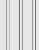
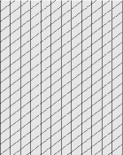
a) $t=0^{-}$	b) $t=0^{+}$	c) $t=+\infty$

Figure 5: Deformation of a slab for model (3.23)

4 General dynamics of curved dislocations

4.1 Preliminary on the dynamics of dislocation curves

At sufficiently low temperature, dislocation curves are contained in the crystallographic planes of the three-dimensional crystal and can only move in those planes. Let us consider a closed and smooth curve $\Gamma_{t}$ moving in the plane $(y_{1},y_{2})$. The evolution of this dislocation can be modelled by a dynamics with normal velocity $c(y,t)$ (see Figure 6).

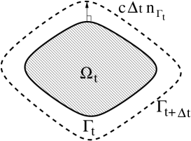
Figure 6: Schematic evolution of a dislocation line $\Gamma_{t}$ by normal velocity $c$ between the times $t$ and $t+\Delta t$.

4.2 Transport formulation of the dynamics

If we want to describe the dynamics of a high number of dislocations curves, it is interesting to describe this dynamics with a single quantity and a single equation. This is the goal of this subsection that we describe heuristically.

Let us consider a smooth closed curve $\Gamma_{0}$ in the plane $(y_{1},y_{2})$ with basis $(e_{1},e_{2})$. The curve $\Gamma_{0}$ can be parametrized by its curvilinear abscissa $s$, such that

$$\Gamma_{0}=\bigcup_{s}\left\{y(s)\right\}.$$

Let us define for $\theta\in{\mathbb{R}}/(2\pi{\mathbb{Z}})$

$$n(\theta)=(\cos\theta)e_{1}+(\sin\theta)e_{2}\quad\mbox{and}\quad\tau(\theta)=(\sin\theta)e_{1}-(\cos\theta)e_{2}.$$

We also define the angle $\theta(s)$ of the tangent to $\Gamma_{0}$ at the point $y(s)$ by

$$\frac{dy}{ds}(s)=\tau(\theta(s))$$

and the curvature $K_{\Gamma_{0}}(y)$ of $\Gamma_{0}$ at the point $y$ by

$$K_{\Gamma_{0}}(y(s))=\frac{d}{ds}(\theta(s)).$$

We introduce the lifting $\widehat{\Gamma}_{0}$ of $\Gamma_{0}$ by

$$\widehat{\Gamma}_{0}=\bigcup_{s}\left\{(y(s),\theta(y(s)))\right\}\quad\quad\subset\quad\quad{\mathbb{R}}^{2}\times({\mathbb{R}}/(2\pi{\mathbb{Z}})).$$

We define the distribution $\delta_{\widehat{\Gamma}_{0}}(y,\theta)$ on the test function $\phi(y,\theta)$ by

$$<\delta_{\widehat{\Gamma}_{0}},\phi>=\int_{\widehat{\Gamma}_{0}}ds\ \phi(y(s),\theta(y(s))).$$

Let us now consider a smooth evolution of the oriented closed curve $\Gamma_{t}$ with normal velocity $c(y,t)$. For any fixed $t$, let us call $s_{\Gamma_{t}}$ the curvilinear absissa of the curve $\Gamma_{t}$ and $s_{\widehat{\Gamma}_{t}}$ the curvilinear abscissa of $\widehat{\Gamma}_{t}$. Then we define the distributions

$$g(y,\theta,t)=\left(\frac{ds_{\Gamma_{t}}}{ds_{\widehat{\Gamma}_{t}}}\right)\ \delta_{\widehat{\Gamma}_{t}}(y,\theta)\quad\mbox{and}\quad\kappa(y,\theta,t)=K_{\Gamma_{t}}(y)\cdot g(y,\theta,t).$$

We can now state the following result (see Theorem 2.1 and Remark 2.3 in [14] and the original system for $(g,\kappa)$ in [8]):

Theorem 4.1

(Transport formulation of the motion by normal velocity)
Under the previous assumptions, the distributions $g,\kappa$ satisfy the compatibility equation

$$\tau\cdot\partial_{y}g+\partial_{\theta}\kappa=0$$ (4.26)

and the system

$$\left\{\begin{array}[]{l}g_{t}+\partial_{y}(cng)+\partial_{\theta}((\tau\cdot\partial_{y}c)g)+c\kappa=0\\ \kappa_{t}+\partial_{y}(cn\kappa)+\partial_{\theta}((\tau\cdot\partial_{y}c)\kappa)-(n\cdot\partial_{y}c)\kappa-(\tau\otimes\tau:\partial_{yy}c)g=0.\end{array}\right.$$ (4.27)

Remark that Theorem 4.1 is only known to be true for smooth evolutions of closed curves. When singularities appear (in general in finite time), we do not know if system (4.27) is still true.

4.3 Dynamics of densities of dislocation curves

We now consider the three dimensional case with the basis $(e_{1},e_{2},e_{3})$. Let us now not only consider dislocations in the particular plane $(y_{1},y_{2})$ for $y_{3}=0$, but also in parallel planes for any $y_{3}=\mbox{constant}$. To this end, let us consider distributions $g(y,\theta,t),\kappa(y,\theta,t)$ with the new notation $y=(y_{1},y_{2},y_{3})$, which are again assumed to satisfy (4.26) and (4.27). To close the system we have to explain how is defined the normal velocity $c(y,t)$ in the case of dislocation dynamics. To this end, we have first to compute the strain $e(y,t)\in{\mathbb{R}}^{3\times 3}_{sym}$ which is solution of the system

$$\left\{\begin{array}[]{l}\mbox{div}\ \sigma=0\quad\mbox{with}\quad\sigma=2\mu e+\lambda(\mbox{trace}(e))Id\\ \mbox{inc}\ e=(\mbox{curl}_{row}\ (b\times\beta))_{sym}\quad\mbox{with}\quad\beta(y,t)=\int_{{\mathbb{R}}\backslash(2\pi{\mathbb{Z}})}d\theta\ \tau(\theta)g(y,\theta,t)\end{array}\right.$$ (4.28)

where the operator $\mbox{inc}\ e$ is obtained, taking first the curl of the column vectors of the matrix $e$, and then the curl of the row vectors of the new matrix. The $\mbox{curl}_{row}$ is the curl of the row vectors of the matrix, and the index $(\ )_{sym}$ means that we consider the symmetric part of the matrix. The quantity $b\otimes\beta$ is called the Nye tensor of dislocation densities, where $b$ is the Burgers vector of the dislocations under consideration. Then, to close the model, we define the normal velocity field by

$$c(y,t)=(b\otimes e_{3}):\sigma(y,t).$$ (4.29)

Relation (4.29) between the normal velocity and the right hand side (called the resolved Peach-Koehler force) is the simplest expression when the drag coefficient is isotropic and taken equal to $1$. Again, if we neglect the short range dynamics, the complete system is (4.26)-(4.27)-(4.28)-(4.29), and can be interpreted as a mean field model, describing the densities of dislocation curves moving in interaction.

Finally, remark that the Groma, Balogh system (1.6) is a particular case of this complete model, when every quantity is invariant in $y_{2}$ and $x_{1}=y_{1}$, $x_{2}=y_{3}$, with the notation $\theta^{\pm}(x_{1},x_{2},t)=g(y_{1},0,y_{3},\pm\pi,t)$.

5 Concluding remarks

The models presented in this paper deal with the dynamics of dislocation densities, and can be seen as a very first (and naive) attempt to derive elasto-visco-plasticity behaviour of crystals. All these models are essentially mean field models, and for instance are not able to explain relations between the stress and the plastic deformation velocity like for instance the typical power-law behaviour

$$\dot{e}^{p}\simeq\pm|\sigma|^{m}$$

with $m$ large. More realistic models should also take into account the complicated short range dynamics, with the possible pinning of dislocations, the creation and destruction of dipoles of dislocations with opposite Burgers vector, and even the possibilities of junctions between dislocations, or the Frank-Read sources and the cross-slip phenomenon. At least, it seems that the framework of kinetic equations for the creation and annihilation of such dipoles should be a promising tool for the modelling of the short range dynamics of dislocations. We hope to investigate this modelling in a future work.

References

- [1] A. Briani, P. Cardaliaguet, R. Monneau, Homogeneization in time for a model with dislocations densities, work in progress.
- [2] M. Cannone, A. El Hajj, R. Monneau, F. Ribaud, Global existence for a system of non-linear and non-local transport equations describing the dynamics of dislocation densities, preprint hal-00266920.
- [3] A. El Hajj, Well-Posedness Theory for a Nonconservative Burgers-Type System Arising in Dislocation Dynamics, SIAM journal of mathematical analysis, 39 (2007), pp. 965-986.
- [4] A. El Hajj, N. Forcadel, A convergent scheme for a non-local coupled system modelling dislocations densities dynamics, Mathematics of Computations, 77 (2008), pp. 789-812.
- [5] I. Groma, P. Balogh, Investigation of dislocation pattern formation in a two-dimensional self-consistent field approximation, Acta Mater, 47 (1999), pp. 3647-3654.
- [6] I. Groma, F. Csikor, M. Zaiser, Spatial correlations and higher-order gradient terms in a continuum description of dislocation dynamics, Acta Mater, 51 (2003), pp. 1271-1281.
- [7] J. R. Hirth, L. Lothe, Theory of dislocations, Second edition, Kreiger publishing company, Florida, 1982.
- [8] T. Hochrainer, M. Zaiser, P. Gumbsch, A self-consistent three-dimensional continuum theory of dislocations, Phil. Mag, 87 (2007), pp. 1261-1282.
- [9] H. Ibrahim, Existence and uniqueness for a non-linear parabolic/Hamilton-Jacobi system describing the dynamics of dislocation densities, accepted for publication in Annales de l’IHP, Non Linear Analysis.
- [10] H. Ibrahim, M. Jazar, R. Monneau, Dynamics of dislocation densities in a bounded channel. Part I: smooth solutions to a singular parabolic system, preprint hal-00281487.
- [11] H. Ibrahim, M. Jazar, R. Monneau, Dynamics of dislocation densities in a bounded channel. Part II: existence of weak solutions to a singular Hamilton-Jacobi strongly coupled system, preprint hal-00281859.
- [12] H. Ishii, S. Koike, Viscosity solutions for monotone systems of second-order elliptic PDEs, Comm. Partial Differential equations, 16 (1991), pp. 1095-1128.
- [13] H. Kozono, Y. Taniuchi, Limiting case of the Sobolev inequality in BMO, with application to the Euler equations, Comm. Math. Phys., 214 (2000), pp: 191-200.
- [14] R. Monneau, A transport formulation of moving fronts and application to dislocations dynamics, Interfaces and Free Boundaries, 9 (2007), pp. 383-409.
- [15] R. Monneau, P. Souganidis, Infinite Laplacian diffusion equations by stochastic time homogenization of a coupled system of first order equations, work in progress.
- [16] V. Volterra, Ann. Sci. Ec. Norm. Sup. Paris 24, (1907), p. 401.