Stochastic self-enrichment, pre-enrichment, and the formation of globular clusters

Abstract

We develop a model for stochastic pre-enrichment and self-enrichment in globular clusters (GCs) during their formation process. GCs beginning their formation have an initial metallicity determined by the pre-enrichment of their surrounding protocloud, but can also undergo internal self-enrichment during formation. Stochastic variations in metallicity arise because of the finite numbers of supernova. We construct an analytic formulation of the combined effects of pre-enrichment and self-enrichment and use Monte Carlo models to verify that the model accurately encapsulates the mean metallicity and metallicity spread among real GCs. The predicted metallicity spread due to self-enrichment alone, a robust prediction of the model, is much smaller than the observed spread among real GCs. This result rules out self-enrichment as a significant contributor to the metal content in most GCs, leaving pre-enrichment as the viable alternative. Self-enrichment can, however, be important for clusters with masses well above $10^{6}~{}{M_{\sun}}$, which are massive enough to hold in a significant fraction of their SN ejecta even without any external pressure confinement. This transition point corresponds well to the mass at which a mass-metallicity relationship (“blue tilt”) appears in the metal-poor cluster sequence in many large galaxies. We therefore suggest that self-enrichment is the primary driver for the mass-metallicity relation. Other predictions from our model are that the cluster-to-cluster metallicity spread decreases amongst the highest mass clusters; and that the red GC sequence should also display a more modest mass-metallicity trend if it can be traced to similarly high mass.

1. Introduction

Globular clusters (GCs) are believed to form in single bursts of star formation within protocluster clouds, producing bound clusters of $10^{4}$ – $10^{7}$ stars which (in most cases) share a single age, metallicity, and element abundance pattern. A near-universal feature of the GCs in any one large galaxy is that they typically follow a bimodal metallicity distribution, a conclusion now based solidly on large statistical samples from many galaxies (e.g. Larsen et al., 2001; Harris et al., 2006; Peng et al., 2006, 2008). The more metal-poor (blue) clusters average ${\mathrm{[Fe/H]}}\sim-1.5$ with a dispersion $\sigma$[Fe/H] $\simeq 0.25$, and metal-richer (red) ones average ${\mathrm{[Fe/H]}}\sim-0.3$ with $\sigma$[Fe/H] $\simeq 0.4$ (Harris et al., 2006).

A more recently discovered second-order feature in the metallicity distributions, that seems particularly to affect the metal-poor component, is a mass-metallicity relation (MMR): the blue clusters become slightly but significantly more metal-rich at progressively higher mass (Harris et al., 2006; Strader et al., 2006; Mieske et al., 2006). No such correlation is seen along the metal-richer, red GC sequence. This feature, also colloquially called a “blue tilt”, is as yet poorly understood, and the various empirical characterizations of the effect are not yet in mutual agreement, even including the extreme claim that it is only an artifact of measurement (Kundu, 2008). Some discussions of the MMR in a few individual galaxies claim to find a systematic correlation of cluster metallicity (color) with mass (luminosity) that spans the entire GC luminosity range (Strader et al., 2006; Spitler et al., 2006; Wehner et al., 2008; Spitler et al., 2008). However, the observational studies based on the biggest statistical samples (thousands of GCs collected from many large E galaxies), and carried out with the best photometric measurement techniques (with careful attention to aperture-size corrections determined from convolutions of the GC profiles with the point-spread function of the image) find that the slope of the MMR becomes most noticeable for the top end of the GC mass range, $M\gtrsim 10^{6}~{}{M_{\sun}}$ (Harris et al., 2006; Mieske et al., 2006; Harris, 2009). For the vast majority of lower-mass clusters, their mean color stays virtually constant and it is debatable whether or not any significant MMR trend exists for $M\lesssim 10^{6}M_{\odot}$.

The fact that the MMR becomes prominent only at the high-mass, high-luminosity end of the GC sequence easily explains why it was not discovered until recently. Massive GCs are rare, and for galaxies with relatively small GC populations (such as the Milky Way, any dwarfs, or any non-giant ellipticals), the GC distribution simply cannot be traced to high enough levels for any systematic change in cluster color with luminosity to be noticed. In the Milky Way, for example, only $\omega$ Centauri is luminous and massive enough to be clearly in the “MMR regime” (Harris et al., 2006). To make the picture additionally puzzling, one or two giant ellipticals seem to have no discernable MMR at any luminosity level (most notably NGC 4472; see Strader et al., 2006; Mieske et al., 2006) and it is not out of the question that the amplitude of the effect may differ from one galaxy to another.

Two other lines of observational evidence have recently emerged to hint more strongly that the systematic properties of GCs start to undergo important changes at around the million-Solar-mass point. One of these is their characteristic radii (usually described by their half-light or effective radius $r_{h}$, which is relatively immune to dynamical evolution). Empirically, $r_{h}$ stays relatively uniform at $r_{h}\simeq 3$ pc for luminosities $L\lesssim 10^{6}~{}{L_{\sun}}$ (corresponding roughly to $M\lesssim 2\times 10^{6}M_{\odot}$), but follows a steeper relation roughly approximated by $r_{h}\sim L^{1/2}$ at higher luminosities (Barmby et al., 2007; Rejkuba et al., 2007; Evstigneeva et al., 2008). This changeover in their structural-parameter plane may smoothly link the most massive GCs with other objects such as UCDs (ultra-compact dwarfs) and the compact nuclei in dwarf ellipticals.

Lastly, evidence gathered from detailed color-magnitude studies and abundance measurements of GCs within the Milky Way (e.g. Bedin et al., 2004; Piotto et al., 2007; Villanova et al., 2007; Milone et al., 2008; Johnson et al., 2008) is now showing that the most massive GCs (again, those typically above about $10^{6}~{}{M_{\sun}}$) are often not the clean “single stellar population” that is classically associated with GCs; instead, they can show two or more distinct sequences in their color-magnitude diagram that are indicators of more than one generation of stars with different chemical abundances.

GC formation models to explain and link all these intriguing characteristics of GCs at different masses are still in rudimentary stages. In this paper, we develop a new quantitative model to address particularly the metallicity distributions of GCs and their systematic change with mass. Our model assumes that a globular cluster in the process of formation can be pre-enriched (that is, its protocluster gas will have an initial heavy-element abundance produced by any generations of stars that happened previously), and also self-enriched (that is, its own first rounds of supernova can further increase its mean metallicity). Our model is intended to explore which of these factors will be dominant in a given situation, and whether the combination is capable of describing the metallicity distribution for real GCs.

Because all timescales associated with the formation and evolution of stars decrease strongly with increasing stellar mass, it is possible for the first high-mass stars in a protocluster to form, live their entire lives, and explode as supernovae (SNe) while the lower-mass stars are still forming. The metals produced from high-mass stars within a protocluster may therefore be incorporated into the lower-mass stars in the same starburst (self-enrichment). In this case, the mean metallicity of the final cluster will reflect several factors including the initial mass function (IMF) of star formation, the efficiency with which the protocloud gas is turned into stars, and the ability of protoclusters to hold on to the metals produced by its SNe (which will be primarily a function of the cloud mass). Because the number of SNe in a protocluster may be subject to small-number statistics, the amount of metal enrichment can be quite stochastic (Cayrel, 1986), resulting in a metallicity spread that itself will be a function of cluster mass.

Recently Strader & Smith (2008) have published a formation model for GCs also based on the idea of self-enrichment. We compare their discussion with ours in more detail in a later section below. We believe that key differences in the assumptions regarding the protocloud structure and formation timescales make our model more physically realistic, and as will be seen below, make it possible to identify the intriguing “transition point” around $10^{6}~{}{M_{\sun}}$ in a more natural way.

2. Star formation and evolution timescales

Previous descriptions of GC and star-cluster formation usually make the zero-order approximation of an “instantaneous starburst” in which the entire stellar IMF springs into place at once. At some level this must be an oversimplification: individual stars have formation times that depend on their mass, and the starburst epoch as a whole will be stretched out over a comparable length of time. Our model of self-enrichment is based instead on the picture that many or most of the high-mass stars form, live, die, and eject their newly formed heavy elements into the surroundings before the low-mass stars have finished assembling a significant fraction of their mass. This scenario, too, must at some level be an idealization, but there is now significant evidence on both the observational and theoretical sides to justify it as a useful first-order approximation.

In the context of globular cluster self-enrichment, “high mass” stars are those that contribute significantly to the total metal production from the stellar population while “low mass” stars are those that are still visible today in a Milky Way GC. The majority of metals are produced in supernovae with progenitor masses of at least $20~{}{M_{\sun}}$ (see Figure 1), while the upper mass limit for “low mass” stars relevant here will be the main-sequence turnoff mass of typical GCs in large galaxies, $M_{TO}\lesssim 1M_{\odot}$. Therefore, the important stellar timescales are the combined formation and evolution timescale of stars of at least $20~{}{M_{\sun}}$ compared to the formation timescales of stars of less than $1~{}{M_{\sun}}$.

The timescales associated with high-mass star formation are extremely short. Churchwell (2002) has shown that the dynamics of molecular outflows in massive star forming regions require very high accretion rates that imply formation timescales of $10^{4}$ – $10^{5}$ yr (see also McKee & Ostriker, 2007, who infer that the formation times for massive stars are $<1$ Myr). Once formed, the evolutionary lifetime of high mass stars is similarly short. Hirschi (2007) calculates lifetimes of $10$ Myr for $20~{}{M_{\sun}}$ stars down to $<6$ Myr for stars of $40~{}{M_{\sun}}$ or greater, and Recchi & Danziger (2005) model combined effect of metal production and stellar ages and find that most metals are released within the first $5$ Myr after the first $100~{}{M_{\sun}}$ star dies (see their figure 6). The timescale for the supernova ejecta to cool is similar, $\sim 7~{}\mathrm{Myr}$ (McKee & Ostriker, 1977). Therefore, even though stars with masses as low as $8~{}{M_{\sun}}$ may explode as supernovae, the key timescale for enrichment is much shorter than the $\sim 50$ Myr lifetime of those stars. In short, a reasonable estimate appears to be that the high-mass part of the IMF can ‘seed’ its surroundings beginning around 5 Myr after formation.

On the other hand, the formation times for low mass stars are much longer. The formation timescale should be approximately the Kelvin-Helmholz time, which rises to $\tau_{KH}\gg 10^{7}$ yr for $M\lesssim 1~{}{M_{\sun}}$ (see figure 4 of Zinnecker & Yorke, 2007). Therefore, even if all stars in a given starburst begin to form simultaneously, the heavy elements from the high mass stars will be ejected into the protocluster cloud while the low mass stars are still collapsing. In fact, simulations that couple hydrodynamics with radiative transfer suggest that feedback from high mass stars critically shapes the low mass IMF itself (Krumholz et al., 2007), providing direct evidence that feedback from high mass stars is important early in the formation of lower mass stars.

These comments still do not include the internal structure of the starburst as a whole. The turbulent medium in which star formation occurs is theoretically expected to result in clumpy star formation, as is seen observationally in dense star-forming regions today (e.g. Feigelson & Townsley, 2008; Townsley et al., 2006), both in the spatial structure of the protocluster and in its temporal evolution over the star formation episode. These studies indicate that the total durations of starbursts in massive, dense protocluster clouds such as the ones we are particularly interested in here are plausibly in the range of $10-20$ Myr. Intervals this long give the low-mass stars that are formed throughout the burst additional time to incorporate metals ejected by the higher-mass stars formed at the onset of the burst. While we will not address the effects of this internal structure on the process of cluster self-enrichment any further, it may be expected to introduce star-to-star metallicity dispersion within the cluster; inhomogeneities of this sort have indeed been detected in some massive GCs (see the references cited above).

3. Stochastic model of self-enrichment

We begin by analyzing the simplest case, where the metal content of clusters comes entirely from self-enrichment, in order to address whether it can be the dominant contributor. We expand this analysis to include contributions from both self-enrichment and pre-enrichment in § 5.

3.1. Mean metallicity

We assume that a globular cluster forms from a molecular cloud of mass $M_{c}$, with a star formation efficiency of $f_{*}$. The stars are distributed according to an IMF $\xi(m)$ of the form

$$\xi(m)\equiv\frac{dn}{dm}=Am^{\alpha}$$ (1)

between a minimum mass $M_{\mathrm{min}}$ and a maximum mass $M_{\mathrm{max}}$ (assumed to be $100~{}{M_{\sun}}$). We assume a Salpeter slope of $\alpha=-2.35$, which is an excellent fit to the observed IMF at $m>1~{}{M_{\sun}}$ (Chabrier, 2003). Although the low mass IMF has large uncertainties, it is known to turn over and therefore contain only a small fraction of the total stellar mass. Our derivation only requires that (a) the high-mass slope of the IMF and (b) the total fraction of mass contained in high mass stars are correct. We may therefore assume a Salpeter IMF with an appropriate low mass cutoff $M_{\mathrm{min}}$ without loss of generality. Chabrier (2003) finds that the mass fraction of stars with $m>9~{}{M_{\sun}}$ is $0.20$; for our adopted IMF, this implies ${M_{\mathrm{min}}}=0.30~{}{M_{\sun}}$.

The normalization constant $A$ can be found from the condition that the integrated mass over the IMF is equal to the total stellar mass $M_{\mathrm{GC}}$ ($=f_{*}M_{c}$):

$$A=\frac{f_{*}M_{c}(\alpha+2)}{{M_{\mathrm{max}}}^{\alpha+2}-{M_{\mathrm{min}}}^{\alpha+2}}.$$ (2)

We assume that all stars above a critical threshold ${M_{\mathrm{SN}}}\sim 8~{}{M_{\sun}}$ explode as SNe. The mass of metals $m_{Z}$ ejected by core collapse supernovae from stars of various progenitor masses $m$ have been calculated by Woosley & Weaver (1995) and Nomoto et al. (1997). Assessment of their data shows that they are reasonably approximated by the relation

$$m_{Z}(m)=(B+Cm)m,$$ (3)

where $B=1.18\%$, $C=0.548\%$, and all masses are in units of $M_{\sun}$. Thus, for example, a $20M_{\odot}$ star would return to its surroundings about $2.4M_{\odot}$ of enriched gas in all heavy elements combined. We assume that these yields do not depend on the metallicity of the progenitor stars, an assumption we justify in § 6.1.2. The total amount of metals produced by SNe within the cloud is therefore

$$M_{Z} = \int_{{M_{\mathrm{SN}}}}^{{M_{\mathrm{max}}}}m_{Z}(m)\xi(m)dm$$ (5)

$$= A\Biggl{[}\frac{B}{\alpha+2}({M_{\mathrm{max}}}^{\alpha+2}-{M_{\mathrm{SN}}}^{\alpha+2})+$$

$$\frac{C}{\alpha+3}({M_{\mathrm{max}}}^{\alpha+3}-{M_{\mathrm{SN}}}^{\alpha+3})\Biggr{]}.$$

The relative importance of stars of different mass can be seen in Figure 1, where we plot the cumulative fraction of total metals contributed by supernovae as a function of the progenitor star mass (i.e. the plotted value is $f(M)=\int_{{M_{\mathrm{SN}}}}^{M}m_{Z}(m)\xi(m)dm/\int_{{M_{\mathrm{SN}}}}^{{M_{\mathrm{max}}}}m_{Z}(m)\xi(m)dm$). Although the IMF rises to low masses, the yield per star drops almost proportionally and so stars with masses near $M_{\mathrm{SN}}$ do not contribute appreciably to the total metal production; almost $80\%$ of the metals come from stars with initial masses of at least $20~{}{M_{\sun}}$.

Figure 1.— Cumulative fraction of metals produced by supernovae with progenitor star masses less than or equal to the given mass. Almost $80\%$ of the metals come from stars with initial masses of at least $20~{}{M_{\sun}}$.

We assume that a fraction $f_{Z}$ of the metals produced stays within the the cloud and ends up incorporated in the formation of the lower-mass stars. For the first stage of our discussion, we assume that $f_{Z}$ is a constant free parameter; we will deal with the more realistic case where $f_{Z}$ depends on the depth of the potential well in § 5. The total metallicity $Z_{c}$ of the gas from which the stars are formed is then

$$Z_{c}=\frac{f_{Z}M_{Z}}{M_{c}},$$ (6)

with $M_{Z}$ taken from equation (5). The resulting metallicity of the low-mass stars that we see in the cluster today, many Gy later, is then

$$\log Z_{c}/{Z_{\sun}}=0.38+\log f_{*}f_{Z},$$ (7)

where we adopt ${Z_{\sun}}=0.016$ (Grevesse & Sauval, 1998; VandenBerg et al., 2007) although the exact value is not critical to our argument. We note that our parameter $f_{Z}$ is essentially similar to the “effective yield” $y_{eff}$ in simple models of chemical evolution (e.g. Pagel & Patchett, 1975; Binney & Merrifield, 1998).

There is no reason to expect either the star formation efficiency $f_{*}$ or the metal retention efficiency $f_{Z}$ to be near unity. Observations indicate that $f_{*}\sim 0.3$ (Lada et al., 1984; Lada & Lada, 2003; Marks et al., 2008). Though $f_{Z}$ is less well constrained by direct observation, we can use the above derivation to constrain the product $f_{*}f_{Z}$. Because the amount of self-enrichment sets only a lower bound to the total GC metallicity, $\log Z_{c}/{Z_{\sun}}$ should not be greater than the mean metal-poor GC metallicity of ${\mathrm{[m/H]}}\simeq-1.25$, which implies $\log f_{*}f_{Z}\leq-1.63$ and thus (if $f_{*}\sim 0.3$) $f_{Z}\lesssim 0.08$.

Furthermore, $f_{*}$ and $f_{Z}$ may in principle vary as a function of cloud mass. For example, the fraction of metals that remain bound to the cloud should increase with the depth of the gravitational potential well, and therefore $f_{Z}$ may increase with mass. This by itself would introduce a positive mass-metallicity relation in the same sense as the observations listed above. We discuss this in more detail in § 5; Strader & Smith (2008) make an argument that is basically similar.

3.2. Metallicity spread

Next, we extend the above derivation to determine the expected cluster-to-cluster dispersion in the GC metallicity distribution, due to the stochastic nature of self-enrichment (Cayrel, 1986). This will turn out to yield an interesting constraint on the relative importance of pre- and self-enrichment.

First we note that the mean number of supernovae in a given GC, $\bar{N}_{\mathrm{SN}}$, is:

$${\bar{N}_{\mathrm{SN}}} = \int_{{M_{\mathrm{SN}}}}^{{M_{\mathrm{max}}}}\xi(m)dm$$ (8)

$$= \frac{A}{\alpha+1}({M_{\mathrm{max}}}^{\alpha+1}-{M_{\mathrm{SN}}}^{\alpha+1}).$$ (9)

The variance in the mass of metals expelled by a single SN is:

$$\sigma^{2}_{m_{Z}}=\left<m_{Z}^{2}\right>-\left<m_{Z}\right>^{2},$$ (10)

where

$$\left<m_{Z}^{2}\right> = \frac{\int_{{M_{\mathrm{SN}}}}^{{M_{\mathrm{max}}}}m_{Z}(m)^{2}\xi(m)dm}{{\bar{N}_{\mathrm{SN}}}}$$

$$= \frac{A}{{\bar{N}_{\mathrm{SN}}}}\Biggl{[}\frac{B^{2}}{\alpha+3}({M_{\mathrm{max}}}^{\alpha+3}-{M_{\mathrm{SN}}}^{\alpha+3})$$

$$+\frac{2BC}{\alpha+4}({M_{\mathrm{max}}}^{\alpha+4}-{M_{\mathrm{SN}}}^{\alpha+4})$$

$$+ \frac{C^{2}}{\alpha+5}({M_{\mathrm{max}}}^{\alpha+5}-{M_{\mathrm{SN}}}^{\alpha+5})\Biggr{]},$$ (12)

and

$$\left<m_{Z}\right>^{2}=\frac{M_{Z}^{2}}{{\bar{N}_{\mathrm{SN}}}^{2}},$$ (13)

with $M_{Z}$ taken from equation (5).

Adding together $\bar{N}_{\mathrm{SN}}$ supernovae, the variance in the total metal mass $M_{Z}$ is

$$\sigma_{M_{Z}}^{2}={\bar{N}_{\mathrm{SN}}}\sigma^{2}_{m_{Z}},$$ (14)

and the relative scatter in the cloud metallicity $Z_{c}$ is:

$$\frac{\sigma_{Z}}{Z_{c}}=\frac{\sigma_{M_{Z}}}{M_{Z}}.$$ (15)

The original cloud mass $M_{c}$ is not observable, but the mass in stars $M_{\mathrm{GC}}$ is. Combining equations (2), (5), and (9) – (15), we find:

$$\frac{\sigma_{Z}}{Z_{c}}=0.059\left(\frac{{M_{\mathrm{GC}}}}{10^{5}~{}{M_{\sun}}}\right)^{-1/2}.$$ (16)

This formulation reveals a remarkable result: the predicted width of the metallicity distribution is a function of only the stellar mass in the globular cluster, independent of the free parameters $f_{*}$ and $f_{Z}$. It is a direct consequence of the fact that higher cluster mass yields larger numbers of SNe and so reduces the statistical fluctuations in the enrichment, regardless of how much gas is lost. This relationship, including normalization, is therefore a robust testable prediction of the model.

3.3. Monte Carlo realization

We next generate a Monte Carlo realization of this process to demonstrate the stochastic effects more explicitly. We begin by randomly sampling cloud masses $M_{c}$ from a mass function for protocluster molecular clouds of the form

$$\frac{dN}{dM_{c}}\propto M_{c}^{-2}$$ (17)

between a minimum mass $M_{0}$ and $M\rightarrow\infty$ (Harris & Pudritz 1994 estimate a slightly shallower slope for the mass function, $\sim-1.6$, but our results are entirely insensitive to its value).

For each cloud, we calculate the mean number of stars expected, $\bar{N}$:

$$\bar{N}=\int_{{M_{\mathrm{min}}}}^{{M_{\mathrm{max}}}}\xi(m)dm$$ (18)

$$=\frac{f_{*}M_{c}(\alpha+2)}{(\alpha+1)}\frac{{M_{\mathrm{max}}}^{\alpha+1}-{M_{\mathrm{min}}}^{\alpha+1}}{{M_{\mathrm{max}}}^{\alpha+2}-{M_{\mathrm{min}}}^{\alpha+2}},$$ (19)

and round it to the nearest integer. We then randomly sample $\bar{N}$ stars from the IMF and find the stellar mass of the cluster, $M_{\mathrm{GC}}$, by taking their sum. Because the input cloud mass $M_{c}$ and the mass obtained from a random sampling of the IMF may not agree, we reassign the cloud mass to $M_{c}={M_{\mathrm{GC}}}/f_{*}$. For each star with mass greater than $M_{\mathrm{SN}}$, we calculate the mass of metals it produces using equation (3), and finally calculate the metallicity of the cloud by summing up the contributions from each SN and multiplying by $f_{Z}/M_{c}$.

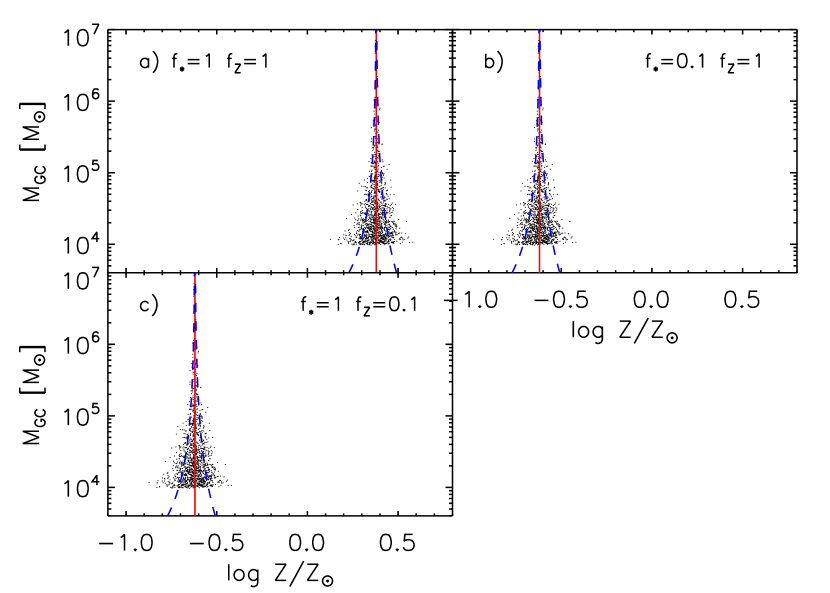
Figure 2.— The stellar mass of globular clusters, $M_{\mathrm{GC}}$ is plotted against their metallicity, $\log Z_{c}/{Z_{\sun}}$. Panels (a), (b), and (c) correspond to the models $f_{*}=1$, $f_{Z}=1$; $f_{*}=0.1$, $f_{Z}=1$; and $f_{*}=1$, $f_{Z}=0.1$ respectively. The mean metallicity from equation (7) is shown as the red solid line, and the predicted dispersion from equation (16) is shown by the blue dashed lines. Dots indicate the Monte Carlo points.

The results of $1500$ Monte Carlo models with a minimum cloud mass of $M_{0}=10^{4}/f_{*}~{}{M_{\sun}}$ (so that the minimum $M_{\mathrm{GC}}$ is constant), along with the results from the analytic derivations, are given in Figure 2. It can be seen that the analytic results and the Monte Carlo samples are completely consistent, and that the free parameters $f_{*}$ and $f_{Z}$ only affect the mean metallicity and not the scatter at a given globular cluster mass.

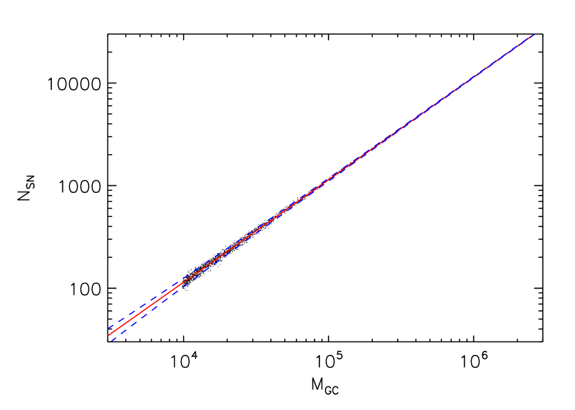
Figure 3.— Number of supernovae per cluster as a function of cluster mass, for the Monte Carlo realization (dots) and the expected mean from the equation (9; red line). The expected Poisson dispersion is shown as the blue dashed lines.

We plot the number of supernovae per cluster in Figure 3. The average is $\simeq 1$ SN for every $100~{}{M_{\sun}}$ of stars formed. Thus, for example, a $10^{5}~{}{M_{\sun}}$ globular cluster – that is, an object that is thought of as a classically “normal” GC – will experience on average $1000$ supernovae during its formation. Note that the spread in cluster metallicities is not simply the Poisson error of the number of supernovae, but is also due to the spread in possible metal contributions of each individual supernova. For example, the relative Poisson error on $1000$ supernovae is $\sim 0.03$, while the actual metallicity spread for clusters of ${M_{\mathrm{GC}}}=10^{5}~{}{M_{\sun}}$ is a factor of two larger.

Lastly, we emphasize that the calculations so far assume a constant gas retention fraction $f_{Z}$, so that the mean self-enrichment is independent of cluster mass. This assumption is rather obviously unrealistic, since at small enough protocluster masses the first few supernovae will remove all the gas and fail to generate any enrichment. We deal with this feature in Section 4 below.

4. Comparison of self-enrichment model with observations

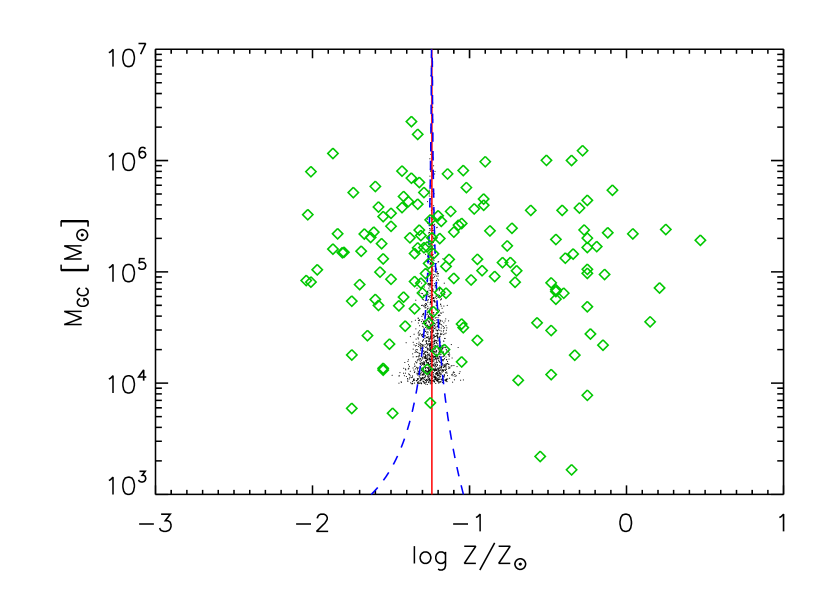
Figure 4.— The red solid line and blue dashed lines show the mean metallicity and its spread predicted from our pure self-enrichment model for $f_{*}=0.3$ and $f_{Z}=0.08$, while the black dots represent 1500 Monte Carlo realizations. The green diamonds represent the observational data from Harris (1996) for Galactic globular clusters, and have been plotted assuming $\log Z/{Z_{\sun}}={\mathrm{[Fe/H]}}+0.25$.

In Figure 4, we compare the metallicities and stellar masses predicted by our self-enrichment model to the observed Milky Way globular clusters (Harris, 1996). When comparing to observations, we assume

$$\log Z/{Z_{\sun}}={\mathrm{[Fe/H]}}+0.25,$$ (20)

with a scatter of $0.1$ dex (e.g. Gratton & Ortolani, 1989; Shetrone et al., 2001; Pritzl et al., 2005; Kirby et al., 2008). We adopt $f_{*}=0.3$ and $f_{Z}=0.08$ in order that the predicted mean metallicity matches the mean metallicity of the observed metal-poor clusters.

The observed metal-poor clusters have a metallicity spread of $\sigma{\mathrm{[Fe/H]}}\approx 0.27$ with no obvious dependence on cluster luminosity. This corresponds to a relative metallicity spread of $\sigma_{Z}/Z=\sigma{\mathrm{[Fe/H]}}\>\ln 10=0.62$. In contrast, the self-enrichment model predicts a relative metallicity spread of only $\sim 0.02$ for clusters with ${M_{\mathrm{GC}}}=10^{6}~{}{M_{\sun}}$, rising to $\sim 0.2$ for very low-mass clusters with ${M_{\mathrm{GC}}}=10^{4}~{}{M_{\sun}}$. In other words, the observed cluster-to-cluster metallicity spread is over an order of magnitude larger than the spread predicted by our self-enrichment model at most cluster masses.

If self enrichment were the dominant source of metals in the metal-poor globular cluster population, then the observed and predicted scatter should be similar, and should be correlated with cluster luminosity. The dramatic discrepancy between the observed and predicted spread, along with the absence of any observed relation between cluster luminosity and metallicity spread, strongly suggests that self-enrichment is not the dominant source of the heavy elements in most metal-poor globular clusters. We conclude that these clusters must have taken their heavy-element compositions from the protocluster clouds before star formation began (“pre enrichment”), and that the observed scatter reflects the variety of environments in which clusters formed.

5. The metal retention efficiency and a predicted MMR

In § 3.1, we derived an upper limit of $f_{Z}\lesssim 0.08$ for the metal retention efficiency based on the mean metallicity of metal-poor globular clusters. Moreover, the upper boundary $f_{Z}\sim 0.08$ corresponds to clusters whose metals are entirely contributed by self-enrichment, while we concluded in § 4 that self-enrichment cannot be the dominant source of metals. It is natural to ask whether such low values for $f_{Z}$ are physically plausible. In this section, we develop a simple energetics argument to obtain a rough estimate for $f_{Z}$ and explore the consequences of the mass-dependent metal retention that naturally arises (see also Dekel & Silk, 1986; Dekel & Woo, 2003, who use a similar energetics argument to examine supernova-driven gas removal from dark matter halo-enshrouded dwarf galaxies).

For simplicity, we assume that the cloud can be approximated by a truncated singular isothermal sphere (TSIS), with a density distribution of the form:

$$\rho(r)=\cases{\frac{M_{c}}{4\pi r_{t}^{3}}\left(\frac{r}{r_{t}}\right)^{-2}&if $r\leq r_{t}$,\cr 0&if $r>r_{t}$,\cr}$$ (21)

where $r_{t}$ is the truncation radius. The potential within the cloud is given by

$$\Phi(r)=\frac{GM_{c}}{r_{t}}\ln r.$$ (22)

The total kinetic energy imparted into the cluster gas is the sum of the energy injected by each supernova. In principle, the important quantity is the number of supernovae that explode within a cooling time, and therefore the supernova rate, rather than the total number, is important. However, in practice the timescale for high-mass star formation is expected to be $<1~{}\mathrm{Myr}$ (see discussion in § 2), sufficiently shorter than the $\sim 7~{}\mathrm{Myr}$ in which a supernova bubble remains hot (McKee & Ostriker, 1977) that all of the cluster supernovae can be approximated as simultaneous.

We next assume that all of the supernova energy is thermalized within the cluster. If each supernova imparts an energy $E_{\mathrm{SN}}$, then the specific kinetic energy $K$ of the gas after thermalization is

$$K=\frac{{\bar{N}_{\mathrm{SN}}}{E_{\mathrm{SN}}}}{M_{c}}.$$ (23)

If the kinetic plus potential energy of the gas is greater than the potential energy at the edge of the cloud, then the gas can escape. This occurs for gas beyond an “escape radius”, $r_{\mathrm{esc}}$:

$$\Phi({r_{\mathrm{esc}}})+K=\Phi(r_{t}).$$ (24)

$$\therefore{r_{\mathrm{esc}}}=r_{t}e^{-{\bar{N}_{\mathrm{SN}}}{E_{\mathrm{SN}}}r_{t}/GM_{c}^{2}}.$$ (25)

Because the enclosed mass in a TSIS is proportional to radius, the fraction of gas within $r_{\mathrm{esc}}$ is simply ${r_{\mathrm{esc}}}/r_{t}$. Assuming that the metals are fully mixed, the metal retention fraction is equal to the gas retention fraction, and is equal to

$$f_{Z}=e^{-{\bar{N}_{\mathrm{SN}}}{E_{\mathrm{SN}}}r_{t}/GM_{c}^{2}}.$$ (26)

$\bar{N}_{\mathrm{SN}}$ scales with $M_{c}$, and is well described by

$${\bar{N}_{\mathrm{SN}}}\approx\frac{{M_{\mathrm{GC}}}}{10^{2}~{}{M_{\sun}}}=\frac{f_{*}M_{c}}{10^{2}~{}{M_{\sun}}}.$$ (27)

Equation (26) can therefore be recast as

$$f_{Z}\approx\exp\left(-\frac{{E_{\mathrm{SN}}}f_{*}r_{t}}{10^{2}~{}{M_{\sun}}GM_{c}}\right).$$ (28)

In Figure 5, we have plotted this relation assuming ${E_{\mathrm{SN}}}=10^{51}~{}\mathrm{erg}$, $f_{*}=0.3$ and $r_{t}=1~{}\mathrm{pc}$. Note that our adopted radius is smaller than the common present-day cluster radius of $3~{}\mathrm{pc}$ due to the expansion of protoclusters upon removal of their gaseous envelope (Baumgardt & Kroupa, 2007); if we adopted a larger value for $r_{t}$, the curve in Figure 5 would maintain its shape but move to proportionally to the right, i.e. to higher mass. It is apparent that $f_{Z}\ll 0.08$ for most cluster masses, as required by our argument that self-enrichment is unimportant.

Figure 5.— Predicted metal retention efficiency $f_{Z}$ as a function of protocluster cloud mass (bottom axis) and final cluster mass (top axis, assuming a star formation efficiency of $f_{*}=0.3$). The solid line is for the fiducial TSIS case, while the other line styles are the predictions for different protocluster density profiles (see § 6.4).

Another way to express this is in terms of the characteristic cloud mass at which metals become efficiently retained, $M^{\mathrm{retain}}_{c}$, which we define to be when the argument of the exponential reaches $-1$:

$$M^{\mathrm{retain}}_{c}=\frac{{E_{\mathrm{SN}}}f_{*}r_{t}}{10^{2}~{}{M_{\sun}}G}.$$ (29)

For the values given, $M^{\mathrm{retain}}_{c}=4\times 10^{7}~{}{M_{\sun}}$. In terms of the observable stellar mass,

$$M^{\mathrm{retain}}_{GC}=f_{*}M^{\mathrm{retain}}_{c}=\frac{{E_{\mathrm{SN}}}f_{*}^{2}r_{t}}{10^{2}~{}{M_{\sun}}G},$$ (30)

and has a value of $M^{\mathrm{retain}}_{GC}=1\times 10^{7}~{}{M_{\sun}}$. This is at the upper range of GC masses, and signals that self-enrichment may begin to become important for the most massive clusters.

The assumption of complete mixing of the enriched gas likely results in an overestimate of $f_{Z}$ (or equivalently, an underestimate of $M^{\mathrm{retain}}$) compared to the real case where the cluster wind contains a disproportionate fraction of the metals produced in the supernovae. The assumption of complete energy thermalization may either result in an overestimate of $f_{Z}$ because it dilutes the supernova energy by the full cluster mass rather than by a smaller fraction of the material, or an underestimate of $f_{Z}$ because it assumes that no energy is lost to radiative cooling. Using more detailed dynamical considerations, Parmentier et al. (1999) argue that protoglobular clouds of significantly lower mass can contain their supernova ejecta than would be expected from simple energy considerations (because of their two-phase model where the enriched gas comes from a previous generation of SNe; see also Morgan & Lake, 1989), indicating that our derivation may underestimate $f_{Z}$ (overestimate $M^{\mathrm{retain}}$). While the relative magnitudes of these effects are difficult to assess without full blown hydrodynamic simulations, their opposite signs reassure us that our results are unlikely to be incorrect by orders of magnitude. Given the approximations inherent in our derivation, we caution against over-interpretation of the detailed form of $f_{Z}$, but expect that the general features — particularly a transition from no self-enrichment at low masses to significant self-enrichment above a threshold GC mass around $M^{\mathrm{retain}}_{GC}$ — are robust.

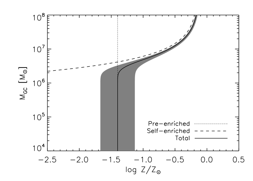
Figure 6.— Predicted globular cluster mass-metallicity relationship assuming a constant pre-enrichment of $\log Z/{Z_{\sun}}=-1.4$ and self enrichment according to our model, with $f_{Z}$ derived from equation (28). The dotted, dashed, and solid lines indicate the metallicity due to pre-enrichment, self-enrichment, and their sum respectively. The shaded region indicates the predicted scatter, assuming that the relative scatter in pre-enriched metallicity is $\sigma{\mathrm{[m/H]}}=0.27$. We have adopted $f_{*}=0.3$; increasing (decreasing) $f_{*}$ will increase (decrease) the threshold mass at which self-enrichment kicks in by a factor of $f_{*}^{2}$ while simultaneously increasing (decreasing) the saturation metallicity at very large $M_{\mathrm{GC}}$ by a factor of $f_{*}$.

In Figure 6, we have plotted the mass-metallicity relation that would be expected if metal-poor GCs are pre-enriched to $\langle{\mathrm{[Fe/H]}}\rangle=-1.65$ ($\log Z/{Z_{\sun}}=-1.4$), and then further self-enriched according to our model, noting again that our adopted supernova yields are independent of the pre-enrichment level. The dotted line indicates the pre-enriched metallicity, the dashed line indicates the metals added by self enrichment, and the solid line is the total predicted metallicity. For these sets of parameters, we see that self-enrichment is predicted to begin contributing at a stellar mass of $\sim 4\times 10^{6}~{}{M_{\sun}}$, very nearly where the observed mass-metallicity relation begins. The shaded region indicates the predicted scatter, where we have assumed that the relative scatter in the pre-enriched metallicities is $\sigma{\mathrm{[m/H]}}=0.27$, as required to fit the observed spread among Milky Way GCs. Because the relative scatter due to stochastic self-enrichment is very small at high masses, the total scatter is entirely dominated by the scatter in the pre-enrichment values. Therefore, the metallicity scatter in absolute units is constant, and the relative scatter becomes smaller at higher mass. Although the details of the mass-metallicity relation are sensitive to the rough estimate of $f_{Z}$, and therefore should not be over-interpreted, it is a clear prediction of our model that the metallicity scatter in dex should decrease as one goes up the mass-metallicity relation, preserving an approximately constant absolute scatter $\sigma_{Z}$.

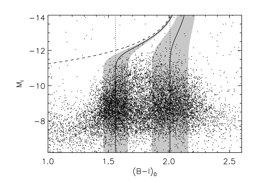
Figure 7.— The lines and shaded regions denote the predictions of our combined pre-enrichment plus self-enrichment model for pre-enrichment values of ${\mathrm{[m/H]}}=-1.6$ with scatter $\sigma{\mathrm{[m/H]}}=0.27$ (left sequence) and ${\mathrm{[m/H]}}=-0.4$ with scatter $\sigma{\mathrm{[m/H]}}=0.40$ (right sequence), translated into the observational color-luminosity space. Line styles are as in Figure 6. We have overplotted the observations of giant elliptical GCs from Harris (2009) for comparison.

We directly compare the observed and predicted MMRs in Figure 7, using the data for 6 giant ellipticals recently remeasured by Harris (2009) from the original data sample of Harris et al. (2006). Here, the metal-poor and metal-rich sequences assume mean pre-enrichments to ${\mathrm{[m/H]}}=-1.6$ and ${\mathrm{[m/H]}}=-0.4$ with scatters of $\sigma{\mathrm{[m/H]}}=0.27$ and $\sigma{\mathrm{[m/H]}}=0.40$ respectively. These mean metallicities are chosen deliberately to match the blue and red GC sequences. We have converted the predicted metallicities and stellar masses into observed absolute magnitudes and colors assuming

$$M_{I}=3.94-2.5\log\frac{L}{L_{\odot}},$$ (31)

$$(B-I)_{0}=2.158+0.375\log\frac{Z}{{Z_{\sun}}}$$ (32)

(Harris et al., 2006). We adopt an $I$-band mass-to-light ratio of $M/L_{I}=1.5~{}{M_{\sun}}/L_{\odot}$, corresponding to $M/L_{V}=2.0~{}{M_{\sun}}/L_{\odot}$ (McLaughlin, 2000) and a mean GC color $V-I=1.0$

The model for the metal-poor clusters shows the same general features as the observations – a constant metallicity and scatter at most luminosities, with an MMR for the most luminous clusters. The observed MMR begins at a lower luminosity than the predicted MMR; this may be related to our overestimate of $M^{\mathrm{retain}}$ compared to the more detailed dynamics in Parmentier et al. (1999), or to mass loss experienced by these clusters since their formation, which would result in an overestimate of their mass today relative to their initial $M_{\mathrm{GC}}$.

An entirely new feature of our model is that it predicts the existence of a MMR for the metal-rich sequence of clusters. Because their pre-enrichment level is $\sim 1$ dex higher, the added factor of self-enrichment has a smaller amplitude than along the blue sequence and cuts in at a slightly higher luminosity, but in principle it should be observable.

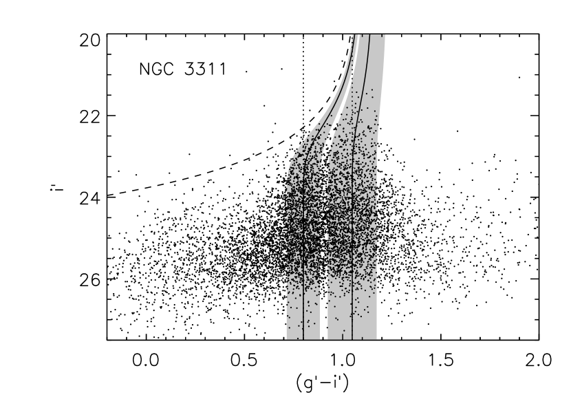
Figure 8.— As in Figure 7, but for globular clusters around NGC 3311 (Wehner et al., 2008). The model assumes a star formation efficiency of $f_{*}=0.2$ and a pre-enrichment level of ${\mathrm{[m/H]}}=-1.2$ for the left sequence, with all other parameters identical to the model in Figure 7.

To date, we do not have much observational material for GCSs where the red sequence is seen to extend to high enough luminosities for its predicted MMR to show up. However, one such galaxy where hints of this effect can be seen is the Hydra cD NGC 3311 (catalog ), shown in Figure 8. The color-magnitude data (Wehner et al., 2008) in $(i^{\prime},g^{\prime}-i^{\prime})$ show the usual presence of the blue and red sequences, but the red sequence displays an unusually high upward extension that may connect to the UCD mass regime at $10^{7}~{}{M_{\sun}}$ and above (Wehner & Harris, 2007) and also shows a small ‘swing’ in mean color further toward the red. We have overplotted our model predictions, assuming the following transformations,

$$i^{\prime}=37.90-2.5\log\frac{L}{L_{\odot}},$$ (33)

$$g^{\prime}-i^{\prime}=1.173+0.311\log\frac{Z}{{Z_{\sun}}}$$ (34)

(based on Peng et al., 2006), and assuming a star formation efficiency $f_{*}=0.2$. The slight reduction in $f_{*}$ from the fiducial value of $f_{*}=0.3$ is required in order to fit the luminosity at which the MMR begins; the sensitive dependence of $M^{\mathrm{retain}}_{GC}$ on $f_{*}$ in equation (30) means that very little change is required. In Figure 8, it can be seen that the strong MMR of the metal-poor population and the mild MMR of the metal-rich population are both well reproduced in our model. We believe that new searches for this MMR effect at the high-mass end of both red and blue sequences would be an extremely effective test of the basic features of our model. They would best be looked for in individual supergiant ellipticals with the largest possible GC samples.

6. Caveats

6.1. Sensitivity to model parameters

Our numerical results may be influenced by the particular values we have adopted for parameters that are either unconstrained or that have significant uncertainty. We address here the influence that each of these parameters has on our numerical and qualitative conclusions.

6.1.1 Initial Mass Function

The IMF is defined by three parameters: $M_{\mathrm{min}}$, $M_{\mathrm{max}}$, and $\alpha$. Changes of $20\%$ in $M_{\mathrm{min}}$ result in changes of $5$–$10\%$ in both the metallicity and its cluster-to-cluster scatter, while changes of $20\%$ in $M_{\mathrm{max}}$ result in changes of $\sim 15\%$ to the metallicity and its scatter.

Flattening the slope of the IMF to $\alpha=-2.1$ increases the mean metallicity by a factor of two, while steepening it to $\alpha=-2.5$ decreases the mean metallicity by $35\%$; however, the changes to the scatter are in both cases less than $25\%$. Because changes to $\alpha$ result in changes to the mean metallicity that are comparable to the observed scatter, scatter in $\alpha$ between clusters could increase the predicted metallicity scatter to the observed level, assuming that the other parameters of the IMF are kept constant. However, this is likely a poor assumption: the fraction of the stellar mass contained in high-mass stars, which determines the number of supernovae and therefore the Poisson scatter, is a more robust quantity than the value of each parameter of the IMF. We conclude that our qualitative results are robust to any realistic uncertainty in the IMF.

6.1.2 Supernova yields

Because our equation for the heavy-element yields is fit to a small number of models in Woosley & Weaver (1995) and Nomoto et al. (1997), there is considerable uncertainty in the parameters. However, our results are completely insensitive to the $B$ parameter in equation (3), and while changes in the $C$ parameter result in proportional changes to the mean predicted metallicity, they have no effect on the metallicity scatter. Another method of effectively changing the supernova yield is to change the minimum supernova progenitor mass, $M_{\mathrm{SN}}$. However, most of the metals are produced by stars with masses $M_{*}\gg{M_{\mathrm{SN}}}$, and so changes in $M_{\mathrm{SN}}$ have no noticable effect on either the mean metallicity or its scatter.

Another potential source of metallicity scatter is from metallicity-dependent supernova yields. If the mass of metals ejected from supernovae depended strongly on the metallicity of the progenitor star, then a small scatter in pre-enrichment levels could be leveraged into a large scatter in final metallicity. However, while the yields of individual elements vary significantly with progenitor metallicity, the total heavy element yields in the supernova models of Woosley & Weaver (1995) are very similar for models with initial metallicities ranging from $10^{-4}$ to $10^{-2}~{}{Z_{\sun}}$, ruling out this possibility.

6.1.3 Star formation efficiency

The predicted metallicity scatter for self enrichment is entirely independent of the mean value of the star formation efficiency, $f_{*}$. Therefore, uncertainty in its value does not alter our conclusions. However, cloud-to-cloud scatter in the star formation efficiency translates directly into metallicity scatter (e.g. Recchi & Danziger, 2005). We therefore cannot rule out a large mass-independent variation in $f_{*}$ as an explanation for the observed metallicity scatter among metal-poor Galactic GCs. However, our metal retention model of § 5 suggests that if self-enrichment were important, there would be an observable MMR for these clusters (only clusters with masses $M\gg M^{\mathrm{retain}}_{GC}$ would exhibit no MMR, a regime that Galactic GCs clearly do not inhabit), which is not observed.

6.1.4 Metal retention efficiency

The metal retention efficiency, $f_{Z}$, occupies a similar role as $f_{*}$: its mean value has no effect on the predicted metallicity scatter in the self enrichment model, but cloud-to-cloud scatter in $f_{Z}$ translates directly into metallicity scatter. We therefore cannot rule out a large mass-independent variation in $f_{Z}$ as an explanation for the observed metallicity scatter, but again note that the MMR that would be expected in the case of self-enrichment is not observed for the Galactic GCs.

Possible scatter in $f_{Z}$ due to stochastic effects is discussed in § 6.3, while scatter in $f_{Z}$ due to scatter in cluster radii at a given mass is discussed in more detail in § 6.6.

6.2. Stellar winds

We have assumed that the global heavy element enrichment and feedback energetics are dominated by core-collapse supernovae (i.e. Types Ib and II). Stellar winds from stars of a wider range of mass contribute significant amounts of some individual elements, but are not believed to dominate the global enrichment and are certainly unimportant energetically in comparison to supernovae (e.g. Oppenheimer & Davé, 2008). If the metal contribution from stellar winds, i.e. from more common lower-mass stars, is higher than currently believed, the metallicity scatter due to self enrichment would be further reduced from the values we derive. Our conclusion that self enrichment produces too little metallicity spread is therefore robust to the heavy element contribution from stellar winds.

6.3. Stochastic metal retention

In the previous picture, all supernovae simultaneously enrich and deposit energy into the protocluster cloud, which becomes well mixed and subsequently loses some fraction of its mass, and so a fraction $f_{Z}$ of each supernova’s metals are retained. Another possible source of scatter is stochastic metal retention. In this picture, the individual supernovae pepper the cloud one at a time, and initially all metals are retained, but eventually one supernova injects enough energy that the total remaining gas can be unbound. Then, without any remaining gaseous envelope, the ejecta from all subsequent supernovae can escape freely and the enrichment stops. In this picture, a fraction $f_{Z}$ of the supernovae have all of their metals retained, while no metals are retained from the remainder. The effective number of supernovae is then reduced from $\bar{N}_{\mathrm{SN}}$to $f_{Z}{\bar{N}_{\mathrm{SN}}}$, and the stochastic relative scatter is increased by a factor of $f_{Z}^{-1/2}$ (this can be thought of as a special case of scatter in $f_{Z}$, which is discussed above). For $f_{Z}=0.08$, the metallicity scatter would be increased by a factor of $3.5$. This factor is well below the order of magnitude required to reconcile the observed and predicted metallicity scatter.

6.4. Protocluster density profile

The adopted isothermal density profile for the protocluster cloud, equation (21), is as steep a profile as can be realistically maintained, and is physically well motivated. However, clouds may exist with slightly shallower density profiles. We therefore briefly expand the derivation of § 5 to generic power-law profiles.

If the density within the truncation radius is given by

$$\rho(r)=\frac{M_{c}(3-\beta)}{4\pi r_{t}^{3}}\left(\frac{r}{r_{t}}\right)^{-\beta},$$ (35)

then for $\beta\neq 2$ the metal retention efficiency is

$$f_{Z}=\left[1-\frac{{\bar{N}_{\mathrm{SN}}}{E_{\mathrm{SN}}}r_{t}(2-\beta)}{GM_{c}^{2}}\right]^{\frac{3-\beta}{2-\beta}}.$$ (36)

We have plotted this relation for a few slopes in Figure 5, in addition to the fiducial $\beta=2$ TSIS case. It is apparent that although the $\beta=2$ case has a unique functional form, it is not “critical” in the sense of showing fundamentally different behaviour; in all cases, the metal retention turns over sharply near $M^{\mathrm{retain}}$. The qualitative effect of a shallower density profile is that a greater fraction of the gas is located near the edge of the cloud where it can be more easily unbound; $f_{Z}$ therefore decreases when $\beta$ is lowered, and shows a sharper transition to the self-enriched regime.

6.5. Mass-radius relation

In § 5 we assumed that all protocluster clouds have a constant radius independent of mass. While this is true for observed GCs with $M\lesssim 2\times 10^{6}M_{\odot}$, a mass-radius relation emerges at higher masses, with radii rising from $r_{h}\simeq 3$ pc at $\sim 10^{6}M_{\odot}$ to $r_{h}\simeq 20$ pc at $\sim 3\times 10^{7}M_{\odot}$ (see Rejkuba et al., 2007; Barmby et al., 2007; Evstigneeva et al., 2008). Assuming that the truncation radius scales similarly as the half-mass radius, we parametrize the mass-radius relation as follows:

$$r_{t}=\cases{r_{t,0}&if ${M_{\mathrm{GC}}}<M_{\mathrm{rad}}$,\cr r_{t,0}\left(\frac{{M_{\mathrm{GC}}}}{M_{\mathrm{rad}}}\right)^{n}&if ${M_{\mathrm{GC}}}\geq M_{\mathrm{rad}}$,\cr}$$ (37)

and examine the consequences on our previous results. The case $n=1/2$ corresponds to simple virial equilibrium and $n=1/3$ to constant density. The available data, accumulated from a combination of the most massive known GCs, UCDs, and dE nuclei, indicate $n\simeq 0.5$ (see the references cited above), which we adopt here.

With this scaling, the metal retention efficiency becomes

$$f_{Z}=\cases{\exp\left(-\frac{M^{\mathrm{retain}}_{GC,0}}{{M_{\mathrm{GC}}}}\right)&if ${M_{\mathrm{GC}}}<M_{\mathrm{rad}}$,\cr\exp\left(-\frac{M^{\mathrm{retain}}_{GC,0}}{M_{\mathrm{rad}}^{n}{M_{\mathrm{GC}}}^{1-n}}\right)&if ${M_{\mathrm{GC}}}\geq M_{\mathrm{rad}}$,\cr}$$ (38)

where we define the critical metal retention mass in the absence of a mass-radius relation $M^{\mathrm{retain}}_{GC,0}$ as in equation (30). The correct critical retention mass $M^{\mathrm{retain}}$ is unchanged if $M_{\mathrm{rad}}>M^{\mathrm{retain}}_{GC,0}$, but otherwise increases by a factor of

$$\frac{M^{\mathrm{retain}}_{GC}}{M^{\mathrm{retain}}_{GC,0}}=\left(\frac{M^{\mathrm{retain}}_{GC,0}}{M_{\mathrm{rad}}}\right)^{\frac{n}{1-n}}.$$ (39)

For $n=1/2$, the exponent in the equation above is just $1$. For example, if we adopt $M_{\mathrm{rad}}=2\times 10^{6}~{}{M_{\sun}}$ as the transition to the mass-radius relation, then the critical retention mass increases by a factor of $\sim 5$ to $M^{\mathrm{retain}}_{GC}=6\times 10^{7}~{}{M_{\sun}}$.

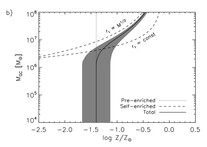
Figure 9.— (a) Metal retention efficiency, $f_{Z}$, as a function of cluster mass, assuming the mass-radius relation of equation (37) (solid line). The dotted line indicates the relationship for clusters of constant radius, as in Figure 5. (b) Predicted mass-metallicity relation, as in Figure 6, but assuming the mass-radius relation of equation (37). The self enrichment level for clusters of constant radius is shown as the lower dashed line.

We have plotted our predicted $f_{Z}$ and mass-metallicity relations in Figure 9, assuming the above mass-radius relation with $n=0.5$ and $M_{\mathrm{rad}}=2\times 10^{6}~{}{M_{\sun}}$. We have also plotted the original relations, where the cluster radius is assumed to be constant, for comparison. We note that the increased radius of high-mass clusters reduces their metal retention because of the shallower potential well, and therefore moves the scale of self-enrichment to higher mass. However, it also results in a shallower mass dependence, more similar to the observed MMRs, and therefore the scale at which self-enrichment becomes apparent (which is approximately where the dotted and dashed lines cross in Figure 9b) is less drastically affected than the factor of $5$ difference in $M^{\mathrm{retain}}_{GC}$.

6.6. Scatter in radius

Lastly, we consider the scatter in cloud radius at a given mass and its effect on $f_{Z}$. The observed scatter in $r_{h}$ for GCs in the Milky Way is $\pm 0.3$ in $\log r_{h}$ (with data from Harris, 1996); i.e., $\sigma_{r}/r\simeq 0.3$. As discussed in § 6.1.4, $f_{Z}$ scatter translates directly into metallicity scatter. We therefore must determine whether the scatter in $r_{t}$ can help reconcile the self-enrichment model with the observed metallicity scatter.

First, we note that the exponential dependence of $f_{Z}$ on $r_{t}$ in equation (28) implies:

$$\frac{\sigma_{f_{Z}}}{f_{Z}}=\frac{\sigma_{r}}{r_{t}}\bigl{|}\ln f_{Z}\bigr{|}.$$ (40)

From § 3.1, we determined $f_{Z}\lesssim 0.08$. With $\sigma_{r}/r_{t}\sim 0.3$, the implied scatter on $f_{Z}$ is $\sigma_{f_{Z}}/f_{Z}\gtrsim 0.75$. This increase in predicted scatter is sufficient to account for the observed metallicity scatter amongst low mass GCs.

While this appears to invalidate our argument in § 3.2 that the magnitude of the observed metallicity scatter rules out self-enrichment as the dominant mode of metal enrichment, there are critical problems with this explanation. First, it is sensitive to the detailed form of $f_{Z}$, which we do not claim is robust. For example, some previous studies of self-enrichment (e.g. Parmentier et al., 1999) have modelled the effects of supernovae as a step-function switch where the protocluster is completely disrupted below a critical mass, but survives intact with full metal retention ($f_{Z}=1$) above it; in such a case, the scatter in $r_{t}$ would not increase the metallicity scatter of the extant clusters at all. Second, the increased scatter is a direct result of the fact that $f_{Z}$ is a function of the depth of the potential well, which is proportional to $M_{c}/r_{t}$. In other words, it is intimately tied to the dependence of $f_{Z}$ on $M_{c}$ and the existence of a mass-metallicity relation; however, no mass-metallicity relation is observed among the low-mass globular clusters. The only possible ways that this could be masked is if $M_{c}\propto r_{t}$ (in marked contrast to the observations, which indicate no mass-radius relation in this mass regime), or if there were a fortuitous cancellation between $f_{*}$ and $f_{Z}$ of the form $f_{*}\propto f_{Z}^{-1}$, which we consider highly unlikely.

We conclude that the overall picture remains most consistent with metallicities that are dominated by pre-enrichment for most GCs.

7. Discussion

7.1. Comparisons with Previous Models

Several previous models for self enrichment have been proposed in the literature (Cayrel, 1986; Morgan & Lake, 1989; Brown et al., 1991; Parmentier et al., 1999; Recchi & Danziger, 2005; Strader & Smith, 2008). Most of these are based on the picture of Fall & Rees (1985), in which the protocluster cloud is a pressure-truncated condensation in the hot halo rather than having its structure determined by gravity (Brown et al., 1991; Parmentier et al., 1999; Recchi & Danziger, 2005). Such models have predicted no mass-metallicity relation (Brown et al., 1991), or a minimal blue tilt that is much weaker than that observed (Recchi & Danziger, 2005), or an inverse MMR in which lower-mass clusters are more metal-rich (Parmentier et al., 1999). These are therefore not adequate for understanding the metallicities of the high-mass clusters whose properties are explained by our model. Most of these models also invoke two distinct star formation episodes: an initial burst of (possibly massive) primordial composition stars whose ejecta pollute the protocluster region, followed by a subsequent burst of star formation from the enriched material. We would classify such a model, in which the metals are produced prior to the burst that creates the stellar cluster we see today, as “pre-enrichment”; however, if the delay between the two bursts is sufficiently short (of order the dynamical time), then this is a matter of semantics rather than a physical difference (e.g. Cayrel, 1986; Recchi & Danziger, 2005).

In the model of Recchi & Danziger (2005), they suggest a number of alternatives in order to obtain the right cluster-to-cluster metallicity scatter $\sigma{\mathrm{[Fe/H]}}$, the most notable of which is to adopt arbitrary and large cluster-to-cluster differences in their “mixing efficiency”, a parameter resembling our gas retention fraction $f_{Z}$ or the effective yield $y_{eff}$. If $f_{Z}$ is primarily determined by the initial cluster mass $M_{c}$, as we suggest that it should, then we view this approach as unlikely. Instead, if $\sigma{\mathrm{[Fe/H]}}$ is due to pre-enrichment, then it can be understood classically as the result of simple chemical evolution such as a “leaky box” model with a suitable effective yield. For the metal-poor GCs or the Milky Way halo stars, a reasonable choice is $y_{eff}\simeq 0.03~{}{Z_{\sun}}$ (Ryan & Norris, 1991; Prantzos, 2003; Vandalsen & Harris, 2004).

For our purposes, the most relevant previous model is that of Strader & Smith (2008), which was specifically created to explain the observed MMR. Their model, like ours, invokes energetic balance between supernova feedback and gravity within a single episode of star formation to produce an MMR via self enrichment. They also put forward the ideas that the transition mass marks the point at which the metals produced by self-enrichment become comparable to those due to pre-enrichment, and that the lack of a corresponding “red tilt” is due to the higher level of pre-enrichment among red sequence GCs. However, there are several key differences between our models. First, in their model the star formation efficiency $f_{*}$ is assumed to vary with mass while the metal retention $f_{Z}$ is constant; instead, we argue that $f_{Z}$ is the physical quantity much more likely to depend strongly on cluster mass, whereas $f_{*}\sim const$. Second, Strader & Smith (2008) derive power-law scalings for the cluster properties such as mass, metallicity, and radius, but do not address their amplitude at all; in contrast, our model is on an absolute scale and explicitly predicts the transition mass from the pre-enriched regime to the self-enriched regime. Third, we predict the existence of a more modest MMR at the high-mass end of the red GC sequence. Finally, and most importantly, they examine the mean trends but not the metallicity scatter between clusters; not only do we explicitly predict the metallicity scatter due to self enrichment, but we use this prediction to conclude that self-enrichment is unimportant among low-mass GCs.

It may be that a combination of ideas from different models would produce an even more realistic match to the real GC distributions. For example, our model predicts a relatively rapid transition from the pre-enriched regime at low cluster masses to a strongly self-enriched regime at high masses, which may be more rapid than observed (note, however, that the mass-radius relation described in § 6.5 results in a shallower MMR). However, a rapid transition from no metal retention to significant metal retention, as in our model, coupled with a star formation efficiency that scales with mass, as in Strader & Smith (2008), might result in a model that is in even better agreement with the observations.

Another possible feature to include in a more general model might be the role of external pressure confinement, which could help the lower-mass clouds keep back some of their SN ejecta (rather than having $f_{Z}\rightarrow 0$ as would be the case if only self-gravity were operating) and possibly allowing the MMR to extend to somewhat lower mass.

7.2. Variation Between Galaxies

At present, the different sets of observations indicate that the amplitude (i.e. the exponent in the scaling $Z_{GC}\propto{M_{\mathrm{GC}}}^{\alpha}$) of the MMR may differ from galaxy to galaxy. The possibility also exists that the blue-sequence MMR may set in at different mass scales and in some cases may be completely absent (Harris et al., 2006; Mieske et al., 2006; Strader et al., 2006; Spitler et al., 2006, 2008; Wehner et al., 2008). In the context of our simple enrichment-based model, these differences would boil down to differences in the degree of self-enrichment at a given cluster mass. The following factors could vary from galaxy to galaxy and therefore affect the observed cluster metallicities:

1. Mass loss from a cluster depends on the strength of the tidal field in which it orbits. Therefore, GCs subjected to stronger tidal fields should have present-day masses less resembling their original $M_{\mathrm{GC}}$. In this case, the MMR imparted at birth would be weakened or destroyed when comparing the present-day masses of the clusters to their metallicity. A possible consequence of this effect would be that the MMR should be stronger in the outer halos of large galaxies.

2. If the protoclusters were bathed in a particularly strong ultraviolet background during formation, (e.g. if the galaxy was undergoing a massive starburst during the main epoch of cluster formation), the gas may have been less able to cool and therefore the star formation efficiency $f_{*}$ may have been reduced. This would result in a lower critical mass $M^{\mathrm{retain}}$ and a lower $Z_{c}$. If $f_{*}$ were reduced sufficiently, the maximum metallicity achievable by self enrichment could even drop below the pre-enriched value, resulting in no MMR at all (see also the discussion about the influence of a UV background in Strader & Smith, 2008).

8. Conclusions

We have developed a model for stochastic self enrichment in globular clusters. This model predicts both the mean metallicity and the cluster-to-cluster spread in metallicities that is expected due to stochastic sampling of the IMF. The predicted metallicity scatter is an order of magnitude smaller than observed for Galactic GCs; this rules out self enrichment as an important contributor to their global metal content and leaves pre-enrichment as the dominant contributor. This conclusion does not depend strongly on the adopted value of any free parameter and is robust to reasonable changes to the shape of the IMF, the supernova heavy element yields, and the details of how metals are retained. Although significant cluster-to-cluster scatter in the star formation efficiency and/or the fraction of metals retained at a given cluster mass could increase the predicted scatter to the observed level, they would most likely be accompanied by a significant mass-metallicity relation at relatively low mass, which is not observed for the Milky Way.

We have used simple energetics to predict how the metal retention efficiency, a key parameter in the self-enrichment model, increases with cluster mass. We propose a combined pre-enrichment plus self-enrichment model, where clusters are pre-enriched to the observed level with significant scatter due to their environment, and then those clusters sufficiently massive that they can retain a significant amount of their supernova ejecta are further self-enriched; the threshold for measurable self-enrichment is predicted to be typically a few $10^{6}~{}{M_{\sun}}$. This model matches the main features of the data so far.

The key features of our model can be summarized as follows:

1. For globular cluster masses less than $\sim 10^{6}~{}{M_{\sun}}$, no MMR is expected for either the blue or red clusters; the mean cluster metallicities should not depend on mass.

2. Along the blue GC sequence, the MMR should ‘kick in’ noticeably for $M_{\mathrm{GC}}$ higher than a few million $M_{\sun}$, reaching ${\mathrm{[m/H]}}\simeq-1$ at ${M_{\mathrm{GC}}}\sim 1-2\times 10^{7}~{}{M_{\sun}}$, corresponding to the most massive known GCs.

3. The cluster-to-cluster metallicity spread $\sigma{\mathrm{[m/H]}}$ remains uniform in the low-mass, pre-enrichment regime, but decreases at higher mass in the MMR regime where self-enrichment becomes most important.

4. A more modest MMR should exist for the red GC sequence, beginning at a few million $M_{\sun}$. In at least one cD galaxy with a very rich GC system (NGC 3311), this effect at the top of the red sequence may have already been seen.

5. Within the context of our model, the main free parameter controlling the level and amplitude of the MMR is the star formation efficiency $f_{*}$. Lowering $f_{*}$ from our baseline value of $0.3$ would reduce the slope of the MMR along both the red and blue GC sequences and might explain the observed differences between galaxies.

Two other physical effects not included in our basic model are a possible correlation of star formation efficiency with cluster mass, and pressure confinement from the gas outside the protoclusters at time of formation. Including these effects properly would allow for a greater range of MMR slopes and onset points and would be an obvious route to explore in a next stage of studying this intriguing effect.

References

- Barmby et al. (2007) Barmby, P., McLaughlin, D. E., Harris, W. E., Harris, G. L. H., & Forbes, D. A. 2007, AJ, 133, 2764
- Baumgardt & Kroupa (2007) Baumgardt, H., & Kroupa, P. 2007, MNRAS, 380, 1589
- Bedin et al. (2004) Bedin, L.R., Piotto, G., Anderson, J., Cassisi, S., King, I.R., Momany, Y., & Carraro, G. 2004, ApJ, 605, L125
- Binney & Merrifield (1998) Binney, J., & Merrifield, M. 1998, Galactic Astronomy (Princeton University Press)
- Brown et al. (1991) Brown, J. H., Burkert, A., & Truran, J. W. 1991, ApJ, 376, 115
- Cayrel (1986) Cayrel, R. 1986, A&A, 168, 81
- Chabrier (2003) Chabrier, G. 2003, in IAU Symposium, Vol. 221, 67
- Churchwell (2002) Churchwell, E. 2002, ARA&A, 40, 27
- Dekel & Silk (1986) Dekel, A., & Silk, J. 1986, ApJ, 303, 39
- Dekel & Woo (2003) Dekel, A. & Woo, J. 2003, MNRAS, 344, 1131
- Evstigneeva et al. (2008) Evstigneeva, E.A., Drinkwater, M.J., Peng, C.Y., Hilker, M., DePropris, R., Jones, J.B., Phillipps, S., Gregg, M.D., & Karick, A.M. 2008, AJ, 136, 461
- Fall & Rees (1985) Fall, M. S., & Rees, M. J. 1985, ApJ, 298, 18
- Feigelson & Townsley (2008) Feigelson, E.D., & Townsley, L.K. 2008, ApJ, 673, 354
- Gratton & Ortolani (1989) Gratton, R.G., & Ortolani, S. 1989, A&A, 211, 41
- Grevesse & Sauval (1998) Grevesse, N., & Sauval, A.J. 1998, Space Sci Rev, 85, 161
- Harris (1996) Harris, W. E. 1996, AJ, 112, 1487
- Harris (2009) Harris, W. E. 2009, ApJ, submitted
- Harris & Pudritz (1994) Harris, W. E., & Pudritz, R. E. 1994, ApJ, 429, 177
- Harris et al. (2006) Harris, W.E., Whitmore, B.C., Karakla, D., Okón, W., Baum, W.A., Hanes, D.A., & Kavelaars, J.J. 2006, ApJ, 636, 90
- Hirschi (2007) Hirschi, R. 2007, A&A, 461, 571
- Johnson et al. (2008) Johnson, C.I., Pilachowski, C.A., Simmerer, J., & Schwenk, D. 2008, ApJ, 681, 1505
- Kirby et al. (2008) Kirby, E.N., Guhathakurta, P., & Sneden, C. 2008, ApJ, 682, 1217
- Krumholz et al. (2007) Krumholz, M. R., Klein, R. I., & McKee, C. F. 2007, ApJ, 656, 959
- Kundu (2008) Kundu, A., AJ, in press (arXiv:0805.0376)
- Lada & Lada (2003) Lada, C.J., & Lada, E.A. 2003, ARA&A, 41, 57
- Lada et al. (1984) Lada, C.J., Margulis, M., & Dearborn, D. 1984, ApJ, 285, 141
- Larsen et al. (2001) Larsen, S.S., Brodie, J.P., Huchra, J.P., Forbes, D.A., & Grillmair, C.J. 2001, AJ, 121, 2974
- Marks et al. (2008) Marks, M., Kroupa, P., & Baumgardt, H. 2008, MNRAS, 386, 2047
- McKee & Ostriker (2007) McKee, C. F., & Ostriker, E.C. 2007, ARA&A, 45, 565
- McKee & Ostriker (1977) McKee, C. F., & Ostriker, J. P. 1977, ApJ, 218, 148
- McLaughlin (2000) McLaughlin, D. E. 2000, ApJ, 539, 618
- Mieske et al. (2006) Mieske, S. et al., 2006, ApJ, 653, 193
- Milone et al. (2008) Milone, A.P. et al. 2008, ApJ, 673, 241
- Morgan & Lake (1989) Morgan, S., & Lake, G. 1989, ApJ, 339, 171
- Nomoto et al. (1997) Nomoto, K., Hashimoto, M., Tsujimoto, T., Thielemann, F.-K., Kishimoto, N., Kubo, Y., & Nakasato, N. 1997, Nuclear Physics A, 616, 79
- Oppenheimer & Davé (2008) Oppenheimer, B. D., & Davé, R. 2008, MNRAS, 387, 577
- Pagel & Patchett (1975) Pagel, B. E. J., & Patchett, B. E. 1975, MNRAS, 175, 595
- Parmentier et al. (1999) Parmentier, G., Jehin, E., Magain, P., Neuforge, C., Noels, A., & Thoul, A. A. 1999, A&A, 352, 138
- Peng et al. (2006) Peng, E.W., Jordán, A., Cóté, P., Blakeslee, J.P., Ferrarese, L., Mei, S., West, M.J., Merritt, D., Milosavljević, M., & Tonry, J.L. 2006, ApJ, 639, 95
- Peng et al. (2008) Peng, E.W., Jordán, A., Cóté, P., Takamiya, M., West, M.J., Blakeslee, J.P., Chen, C.-W., Ferrarese, L., Mei, S., Tonry, J.L., & West, A.A. 2008, ApJ, 681, 197
- Piotto et al. (2007) Piotto, G., Bedin, L.R., Anderson, J., King, I.R., Cassisi, S., Milone, A.P., Villanova, S., Pietrinferni, A., & Renzini, A. 2007, ApJ, 661, L53
- Prantzos (2003) Prantzos, N. 2003, A&A, 404, 211
- Pritzl et al. (2005) Pritzl, B.J. Venn, K.A., & Irwin, M. 2005, AJ, 130, 2140
- Recchi & Danziger (2005) Recchi, S., & Danziger, I. J. 2005, A&A, 436, 145
- Rejkuba et al. (2007) Rejkuba, M., Dubath, P., Minniti, D., & Meylan, G. 2007, A&A, 469, 147
- Ryan & Norris (1991) Ryan, S. G., & Norris, J. E. 1991, AJ, 101, 1865
- Shetrone et al. (2001) Shetrone, M.D., Cóté, P., & Sargent, W.L.W. 2001, ApJ, 548, 592
- Spitler et al. (2006) Spitler, L.R., Larsen, S.S., Strader, J., Brodie, J.P., Forbes, D.A., & Beasley, M.A. 2006, AJ, 132, 1593
- Spitler et al. (2008) Spitler, L.R., Forbes, D.A., & Beasley, M.A. 2008, MNRAS, in press (arXiv:0806.4390)
- Strader et al. (2006) Strader, J., Brodie, J.P., Spitler, L., & Beasley, M.A. 2006, AJ, 132, 2333
- Strader & Smith (2008) Strader, J., & Smith, G.H. 2008, AJ, 136, 1828
- Townsley et al. (2006) Townsley, L.K., Broos, P.S., Feigelson, E.D., Garmire, G.P. & Getman, K.V. 2006, AJ, 131, 2164
- Vandalsen & Harris (2004) Vandalsen, M. L., & Harris, W. E. 2004, AJ, 127, 368
- VandenBerg et al. (2007) VandenBerg, D.A., Gustaffson, B., Edvardsson, B., Eriksson, K., & Ferguson, J. 2007, ApJ, 666, L105
- Vesperini et al. (2003) Vesperini, E., Zepf, S. E., Kundu, A., & Ashman, K. M. 2003, ApJ, 593, 760
- Villanova et al. (2007) Villanova, S. et al. 2007, ApJ, 663, 296
- Weidner et al. (2007) Weidner, C., Kroupa, P., Nurnberger, D. E. A., & Sterzik, M. F. 2007, MNRAS, 376, 1879
- Wehner & Harris (2007) Wehner, E. M. H., & Harris, W. E. 2007, ApJ, 668, L35
- Wehner et al. (2008) Wehner, E.M.H., Harris, W.E., Whitmore, B.C., Rothberg, B., & Woodley, K.A. 2008, ApJ, 681, 1233
- Woosley & Weaver (1995) Woosley, S. E., & Weaver, T. A. 1995, ApJS, 101, 181
- Zinnecker & Yorke (2007) Zinnecker, H., & Yorke, H. W. 2007, ARA&A, 45, 481