Complexity, Heegaard diagrams and generalized Dunwoody manifolds

Abstract

We deal with Matveev complexity of compact orientable 3-manifolds represented via Heegaard diagrams. This lead us to the definition of modified Heegaard complexity of Heegaard diagrams and of manifolds. We define a class of manifolds which are generalizations of Dunwoody manifolds, including cyclic branched coverings of two-bridge knots and links, torus knots, some pretzel knots, and some theta-graphs. Using modified Heegaard complexity, we obtain upper bounds for their Matveev complexity, which linearly depend on the order of the covering. Moreover, using homology arguments due to Matveev and Pervova we obtain lower bounds.
Mathematics Subject Classification 2000: Primary 57M27, 57M12; Secondary 57M25.
Keywords: complexity of 3-manifolds, Heegaard diagrams, Dunwoody manifolds, cyclic branched coverings

1 Introduction and preliminaries

The notion of complexity for compact 3-dimensional manifolds has been introduced by S. Matveev via simple spines. We briefly recall its definition (for further reference see [13, 14]).

A polyhedron $P$ embedded into a compact connected 3-manifold $M$ is called a spine of $M$ if $M$ collapses to $P$ in the case $\partial M\neq\emptyset$, and if $M-{\rm Int}(B)$ collapses to $P$ in the case $\partial M=\emptyset$, where $B$ is a closed 3-ball in $M$. Moreover, a spine $S$ is said to be almost simple if the link of each point $x\in S$ can be embedded into $K_{4}$, a complete graph with four vertices. A true vertex of an almost simple spine $S$ is a point $x\in S$ whose link is homeomorphic to $K_{4}$.

The complexity $c(M)$ of $M$ is the minimum number of true vertices among all almost simple spines of $M$. Complexity is additive under connected sum of manifolds and, for any integer $n\geqslant 0$, there are only finitely many closed prime manifolds with complexity $n$.

In the closed orientable case there are only four prime manifolds of complexity zero which are ${\bf S}^{3}$, $\mathbb{RP}^{3}$, ${\bf S}^{2}\times{\bf S}^{1}$, and $L_{3,1}$. Apart from these special cases, it can be proved that $c(M)$ is the minimum number of tetrahedra needed to obtain $M$ by pasting together their faces (via face paring). A complete classification of closed orientable prime manifolds up to complexity 12 can be found in [15, 16].

In general, the computation of the complexity of a given manifold is a difficult problem. So, two-sided estimates of complexity become important, especially when dealing with infinite families of manifolds (see, for example, [14, 17, 25]).

By [14, Theorem 2.6.2], a lower bound for the complexity of a given manifold can be obtained via the computation of its first homology group. Moreover, for a hyperbolic manifold a lower bound can be obtained via volume arguments (see [14, 17, 25]). On the other hand, upper bound can be found using triangulations.

In this paper we deal with the possibility of calculating complexity via Heegaard decompositions. This way of representing 3-manifold has revealed to be very useful in different contests. So, it is natural to wonder whereas it is possible to calculate complexity via Heegaard diagrams. In Section 2 we use Heegaard diagrams to define modified Heegaard complexity of compact 3-manifolds and compare this notion with Matveev complexity. A widely studied family of manifolds, defined via Heegaard diagrams, is the one of Dunwoody manifolds (see [8]). This family coincides with the class of strongly-cyclic branched coverings of $(1,1)$-knots (see [6]), including, for example, 2-bridge knots, torus knots and some pretzel knots. In Section 3 we construct a class of manifolds that generalizes the class of Dunwoody manifolds, including other interesting class of manifolds such as cyclic-branched coverings of 2-component 2-bridge links. In Section 4, using modified Heegaard complexity, we obtain two-sided estimates for the complexity of some families of generalized Dunwoody manifolds.

2 Heegaard diagrams and complexity

In this section we introduce the notions of modified complexity for Heegaard diagrams and for manifolds, comparing these notions with Matveev complexity of manifolds. Let us start by recalling some definitions.

Let $\Sigma_{g}$ be a closed, connected, orientable surface of genus $g$. A system of curves on $\Sigma_{g}$ is a (possibly empty) set of simple closed curves $\mathcal{C}=\{\gamma_{1},\ldots,\gamma_{k}\}$ on $\Sigma_{g}$ such that $\gamma_{i}\cap\gamma_{j}=\emptyset$ if $i\neq j$, for $i,j=1,\ldots,k$. Moreover, we denote with $V(\mathcal{C})$ the set of connected components of the surface obtained by cutting $\Sigma_{g}$ along the curves of $\mathcal{C}$. The system $\mathcal{C}$ is said to be proper if all elements of $V(\mathcal{C})$ have genus zero, and reduced if either $|V(\mathcal{C})|=1$ or $V(\mathcal{C})$ has no elements of genus zero. Thus, $\mathcal{C}$ is: (i) proper and reduced if and only if it consists of one element of genus $0$; (ii) non-proper and reduced if and only if all its elements are of genus $>0$; (iii) proper and non-reduced if and only if it has more than one element and all of them are of genus $0$; (iv) non-proper and non-reduced if and only if it has at least one element of genus $0$ and at least one element of genus $>0$. Note that a proper reduced system of curves on $\Sigma_{g}$ contains exactly $g$ curves.

We denote by $G(\mathcal{C})$ the graph which is dual to the one determined by $\mathcal{C}$ on $\Sigma_{g}$. Thus, vertices of $G(\mathcal{C})$ correspond to elements of $V(\mathcal{C})$ and edges correspond to curves of $\mathcal{C}$. Note that loops and multiple edges may arise in $G(\mathcal{C})$.

A compression body $K_{g}$ of genus $g$ is a 3-manifold with boundary, obtained from $\Sigma_{g}\times[0,1]$ by attaching a finite set of 2-handles $Y_{1},\ldots,Y_{k}$ along a system of curves (called attaching circles) on $\Sigma_{g}\times\{0\}$ and filling in with balls all the spherical boundary components of the resulting manifold, except from $\Sigma_{g}\times\{1\}$ when $g=0$. Moreover, $\partial_{+}K_{g}=\Sigma_{g}\times\{1\}$ is called the positive boundary of $K_{g}$, while $\partial_{-}K_{g}=\partial K_{g}-\partial_{+}K_{g}$ is called negative boundary of $K_{g}$. Notice that a compression body is a handlebody if an only if $\partial_{-}K_{g}=\emptyset$, i.e., the system of the attaching circles on $\Sigma_{g}\times\{0\}$ is proper. Obviously homeomorphic compression bodies can be obtained with (infinitely many) non isotopic systems of attaching circles.

Remark 1

If the system of attaching circles is not reduced then it contains at least one reduced subsystem of curves determining the same compression body $K_{g}$. Indeed, if $\mathcal{C}$ is the system of attaching circles, denote with $V^{+}(\mathcal{C})$ the set of vertices of $G(\mathcal{C})$ corresponding to the components with genus greater then zero, and with $\mathcal{A}(\mathcal{C})$ the set consisting of all the graphs $T_{i}$ such that:

• $T_{i}$ is a subgraph of $G(\mathcal{C})$;

• if $V^{+}(\mathcal{C})=\emptyset$ then $T_{i}$ is a maximal tree in $G(\mathcal{C})$;

• if $V^{+}(\mathcal{C})\neq\emptyset$ then $T_{i}$ contains all the vertex of $G(\mathcal{C})$ and each component of $T_{i}$ is a tree containing exactly a vertex of $V^{+}(\mathcal{C})$.

Then, for any $T_{i}\in\mathcal{A}(\mathcal{C})$, the system of curves obtained by removing from $\mathcal{C}$ the curves corresponding to the edges of $T_{i}$ is reduced and determines the same compression body. Note that this operation corresponds to removing complementary 2- and 3-handles. Moreover, it is easy to see that if $\partial_{-}K_{g}$ has $k$ boundary components with genus $g_{1},\ldots,g_{k}$ then

$$|E(T_{i})|=|\mathcal{C}|-n-k+1+\sum_{j=1}^{k}g_{j}$$

for each $T_{i}\in\mathcal{A}(\mathcal{C})$, where $E(T_{i})$ denotes the edge set of $T_{i}$.

Let $M$ be a compact, connected, orientable 3-manifold without spherical boundary components. A Heegaard surface of genus $g$ for $M$ is a surface $\Sigma_{g}$ embedded in $M$ such that $M-\Sigma_{g}$ consists of two components whose closures $K^{\prime}$ and $K^{\prime\prime}$ are (homeomorphic to), respectively, a genus $g$ handlebody and a genus $g$ compression body.

The triple $(\Sigma_{g},K^{\prime},K^{\prime\prime})$ is called Heegaard splitting of $M$. It is a well known fact that each compact connected orientable 3-manifold without spherical boundary components admits a Heegaard splitting.

Remark 2

By [14, Proposition 2.1.5] the complexity of a manifold is not affected by puncturing it. So, with the aim of computing complexity, it is not restrictive assuming that the manifold does not have spherical boundary components.

On the other hand, a triple $H=(\Sigma_{g},\mathcal{C^{\prime}},\mathcal{C^{\prime\prime}})$, where $\mathcal{C^{\prime}}$ and $\mathcal{C^{\prime\prime}}$ are two systems of curves on $\Sigma_{g}$, such that they intersect transversally and $\mathcal{C^{\prime}}$ is proper, uniquely determines a 3-manifold $M_{H}$ which corresponds to the Heegaard splitting $(\Sigma_{g},K^{\prime},K^{\prime\prime})$, where $K^{\prime}$ and $K^{\prime\prime}$ are respectively the handlebody and the compression body whose attaching circles correspond to the curves in the two systems. Such a triple is called Heegaard diagram for $M_{H}$.

We denote by $\Gamma(H)$ the graph embedded in $\Sigma_{g}$, obtained from the curves of $\mathcal{C^{\prime}}\cup\mathcal{C^{\prime\prime}}$, and by $\mathcal{R}(H)$ the set of regions of $\Gamma(H)$. Note that $\Gamma(H)$ has two types of vertices: singular vertices which are 4-valent and non-singular ones which are 2-valent. A diagram $H$ is called reduced if both the systems of curves are reduced. If $H$ is non-reduced, then we denote by $\textup{Rd}(H)$ the set of reduced Heegaard diagrams obtained from $H$ by reducing the system of curves.

In [14, Section 7.6] the notion of complexity of a reduced Heegaard diagram $H$ of a genus two closed manifold is defined as the number $c(H)$ of singular vertices of the graph $\Gamma(H)$. Moreover the author proved that $c(M_{H})\leqslant c(H)$.

Now we extend this definition to the general case, slightly modifying it in order to obtain a better estimate for the complexity of $M_{H}$.

The modified complexity of a reduced Heegaard diagram $H$ is

$$\widetilde{c}(H)=c(H)-\max\,\{n(R)\mid R\in\mathcal{R}(H)\},$$

where $n(R)$ denotes the number of singular vertices contained in the region $R$, and the modified complexity of a (non-reduced) Heegaard diagram $H$ is

$$\widetilde{c}(H)=\min\,\{\tilde{c}(H^{\prime})\mid H^{\prime}\in\textup{Rd}(H)\}.$$

We define the modified Heegaard complexity of a closed connected 3-manifold $M$ as

$$\widetilde{c}(M)=\min\,\{\widetilde{c}(H)\mid H\in\mathcal{H}(M)\},$$

where $\mathcal{H}(M)$ is the set of all Heegaard diagrams of $M$.

The following statement generalizes a result of [14, Proposition 2.1.8] (for the case of reduced diagrams of closed manifolds) and [3] (for case of Heegaard diagrams arising from gem representation of closed manifolds).

Proposition 3

If $M$ is a compact connected 3-manifold then

$$c(M)\leqslant\widetilde{c}(M).$$

Proof. Let $H=(\Sigma_{g},\mathcal{C}^{\prime},\mathcal{C}^{\prime\prime})$ be a Heegaard diagram of $M$ and let $(\Sigma_{g},K^{\prime},K^{\prime\prime})$ be the associated Heegaard splitting. We want to prove that $c(M)\leqslant\widetilde{c}(H)$. From the definition of modified complexity it is clear that we can suppose that $H$ is reduced. If $\partial M=\emptyset$ then the statement is given in [14, Proposition 2.1.8]. For the case $\partial M\neq\emptyset$ the same proof works because of the following reason. The simple polyhedron obtained as the union of $\Sigma_{g}$ with the core of the 2-handles of $K^{\prime}$ and $K^{\prime\prime}$ is a spine with $c(H)$ singular vertices of $M-{\rm Int}(B)$, where $B\subset K^{\prime}$ is a closed ball. Since $\partial M$ is contained in $K^{\prime\prime}$, a spine for $M$ can be obtained by connecting $\partial B$ with $\partial M$ via pinching a region of $\mathcal{R}(H)$.   

By results of [4], the upper bound in Proposition 3 becomes an equality for the $69$ closed connected prime orientable 3-manifolds admitting a (colored) triangulation with at most $28$ tetrahedra. As far as we know there is no example where the strict inequality holds.

Conjecture 4

For every compact connected orientable 3-manifold $M$ the equality $c(M)=\widetilde{c}(M)$ holds.

3 Generalized Dunwoody manifolds

In this section we define a class of manifolds that generalizes the class of Dunwoody manifolds introduced in [8].

A Dunwoody diagram is a trivalent regular planar graph, depending on six integers $a,b,c,n,r,s$, such that $n>0$, $a,b,c\geqslant 0$ and $d=2a+b+c>0$, and it is defined as follows (see Figure 1).

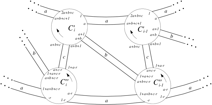
Figure 1: A Dunwoody diagram.

It contains $n$ internal circles $C^{\prime}_{1},\ldots,C^{\prime}_{n}$, and $n$ external circles $C^{\prime\prime}_{1},\ldots,C^{\prime\prime}_{n}$, each having $d$ vertices. The circle $C^{\prime}_{i}$ (resp. $C^{\prime\prime}_{i}$) is connected to the circle $C^{\prime}_{i+1}$ (resp. $C^{\prime\prime}_{i+1}$) by $a$ parallel arcs, to the circle $C^{\prime\prime}_{i}$ by $c$ parallel arcs and to the circle $C^{\prime\prime}_{i-1}$ by $b$ parallel arcs, for every $i=1,\ldots,n$ (subscripts mod $n$). We denote by $\mathcal{A}$ the set of arcs, and by $\mathcal{B}$ the set of circles. By gluing the circle $C^{\prime}_{i}$ to the circle $C^{\prime\prime}_{i+s}$ in the way that equally labelled vertices are identified together (see Figure 1 for the labelling), we obtain a Heegaard diagram $H(a,b,c,n,r,s)=(\Sigma_{n},\mathcal{C}^{\prime},\mathcal{C}^{\prime\prime})$, where $\mathcal{C}^{\prime}$ is the proper, reduced system of curves arising from $\mathcal{B}$, containing $n$ curves, and $\mathcal{C}^{\prime\prime}$ is the system of curves arising from $\mathcal{A}$, containing $m>0$ curves. Observe that the parameters $r$ and $s$ can be considered mod $d$ and mod $n$ respectively. We call $H(a,b,c,r,n,s)$ closed Dunwoody diagram. The generalized Dunwoody manifold $M(a,b,c,n,r,s)$ is the manifold $M_{H(a,b,c,n,r,s)}$.

Since both the diagram and the identification rule are invariant with respect to an obvious cyclic action of order $n$, the generalized Dunwoody manifold $M(a,b,c,n,r,s)$ admits a cyclic symmetry of order $n$.

Remark 5

It is easy to observe that diagrams $H(a,b,c,r,n,s)$ and $H(a,c,b,d-r,n,n-s-1)$ are isomorphic, so they represent the same manifold.

A generalized Dunwoody manifold $M(a,b,c,n,r,s)$ is a Dunwoody manifold when the system $\mathcal{C}^{\prime\prime}$ of curves arising from $\mathcal{A}$ is proper and reduced. In this case $H(a,b,c,n,r,s)$ is a “classical” Heegaard diagram (see [11]) and therefore all Dunwoody manifolds are closed.

As proved in [5], the class of Dunwoody manifolds coincides with the class of strongly-cyclic branched covering of $(1,1)$-knots. So, in particular, it contains all cyclic branched coverings of 2-bridge knots. It is not known if cyclic branched coverings of 2-bridge links (with two components) admit representations as Dunwoody manifolds, but they surely are generalized Dunwoody manifolds. This can be shown by introducing a polyhedral description for generalized Dunwoody manifolds.

Figure 2: Polyhedral description of generalized Dunwoody manifolds.

Referring to Figure 2, let $B$ be the closed unitary 3-ball in $\mathbb{R}^{3}$ and consider on its boundary $n$ equally spaced meridians $m_{1},\ldots m_{n}$ joining the north pole $N=(0,0,1)$ with the south pole $S=(0,0,-1)$. Subdivide each meridian $m_{i}$ into $2a+b$ arcs with endpoints $P_{i,j}$, $j=0,\ldots,2a+b$, such that $P_{i,0}=N$ and $P_{i,2a+b}=S$. Let $t_{i}\in\partial B$ be the shortest arc connecting $P_{i,a+b}$ with $P_{i+1,a}$, for $i=1,\ldots,n$. We subdivide $t_{i}$ into $c$ arcs with endpoints $Q_{i,j}$ for $j=0,\ldots,c$ such that $Q_{i,0}=P_{i,a+b}$ and $Q_{i,c}=P_{i+1,a}$. In this way $\partial B$ is subdivided into $2n$ $d$-gons with $d=2a+b+c$. We denote by $R_{1},\ldots,R_{n}$ the $d$-gons containing the north pole $P_{i,0}=N$ and by $R^{\prime}_{1},\ldots,R^{\prime}_{n}$ the $d$-gons containing the south pole. Moreover, let

$$P^{\prime}_{i,0}=\begin{cases}P_{i,2a+b-r}&0\leqslant r\leqslant a,\\ Q_{i,r-a}&a\leqslant r\leqslant a+c,\\ P_{i+1,r-c}&a+c\leqslant r\leqslant 2a+b+c.\end{cases}$$

According to this definition $P^{\prime}_{i,0}$ is a point on the boundary of $R^{\prime}_{i}$ obtained from $S$ by giving a combinatorial $r$-twist in counterclockwise direction to the region $R^{\prime}_{i}$.

We glue $R_{i}$ with $R^{\prime}_{i+s}$ by an orientation reversing homeomorphism matching the vertices of $R_{i}$ with the ones of $R^{\prime}_{i+s}$ such that $P_{i,0}\in R_{i}$ is identified with $P^{\prime}_{i+s,0}\in R^{\prime}_{i+s}$. In this way we obtain a closed connected orientable pseudomanifold $\widehat{M}(a,b,c,n,r,s)$ with a finite number of singular points whose stars are cones over closed connected orientable surfaces. By removing the interior of a regular neighboorhood of each singular point we get a compact connected orientable 3-manifold with (possibly empty) non-spherical boundary components, which is homeomorphic to the generalized Dunwoody manifold $M(a,b,c,n,r,s)$.

As a particular case, an $n$-fold cyclic branched covering of a 2-bridge link/knot $\mathbf{b}(\alpha,\beta)$ is $M(\beta,\alpha-2\beta,1,n,2\beta+1,s)$ where $s=(-1)^{\beta}$ if $\mathbf{b}(\alpha,\beta)$ is a knot (i.e. $\alpha$ is odd) and $s\neq 0$ if $\mathbf{b}(\alpha,\beta)$ has two components (i. e. $\alpha$ is even) (see [20, 21]).

4 Upper and lower bounds

In this section we calculate the modified complexity of a closed Dunwoody diagram in order to find upper bounds for the complexity of some families of generalized Dunwoody manifolds. For $n=1$, the generalized Dunwoody manifold is a a lens space (including ${\bf S}^{2}\times{\bf S}^{1}$ and ${\bf S}^{3}$) in the closed case and a solid torus in the case with boundary. Since the complexity of these manifolds has been already studied (see [14, Section 2.3.3]), we will always suppose $n>1$.

Theorem 6

Let $H=H(a,b,c,n,r,s)=(\Sigma_{n},\mathcal{C^{\prime},\mathcal{C}^{\prime\prime}})$ be a closed Dunwoody diagram, and $d=2a+b+c$. For each $\gamma\in\mathcal{C}^{\prime\prime}$ define $n(\gamma)$ as the number of singular vertices contained in the cycle determined by $\gamma$ in $\Gamma(H)$. Then, with the notation of Remark 1 we have:

$$\widetilde{c}(H)=nd-\max\left\{n(R)+\sum_{\gamma\in E(T)}n(\gamma)\mid T\in\mathcal{A}(\mathcal{C}^{\prime\prime}),R\in\mathcal{R}(H_{T})\right\},$$

where $E(T)$ is the edge set of the graph $T$ and $H_{T}$ is the element of $\textup{Rd}(H)$ obtained by removing from $\mathcal{C}^{\prime\prime}$ the curves belonging to $T$.

Proof. By construction the system $\mathcal{C}^{\prime}$ is proper and reduced. The statement follows from the definition of modified complexity and Remark 1.   

This result allows us to find upper bounds for the modified complexity (and so for Matveev complexity) of generalized Dunwoody manifolds. In the following subsections we specialize the estimates to the cases of some important families.

4.1 Dunwoody manifolds

Proposition 7

Let $M=M(a,b,c,n,r,s)$ be a Dunwoody manifold. Then

• If $abc>0$ then

  $$c(M)\leqslant\left\{\begin{array}[]{ll}n(2a+b+c)-\max(2n,6)&\textup{ if }r\neq-b,-b\pm 1,\\ n(2a+b+c)-\max(2n,5)&\textup{ if }r=-b\pm 1.\\ \end{array}\right.$$

• If $abc=0$ and $\min(a,b+c)=0$ then

  $$c(M)\leqslant\left\{\begin{array}[]{ll}n(2a+b+c-4)&\textup{ if }r\neq-b,-b\pm 1,\\ n(2a+b+c-3)&\textup{ if }r=-b\pm 1.\\ \end{array}\right.$$

• If $abc=0$ and $\min(a,b+c)>0$ then

  $$c(M)\leqslant\left\{\begin{array}[]{ll}n(2a+b+c-2)&\textup{ if }n>3,\\ n(2a+c)-\max(2n,8-2k_{0})&\textup{ if }n=2,3,\,b=0\textup{ and }s=0,\\ n(2a+b)-\max(2n,8-k_{0}-k_{1})&\textup{ if }n=2,c=0\textup{ and }s=0,\\ n(2a+b)-\max(2n,8-k_{0})&\textup{ if }n=3,c=0\textup{ and }s=0,\\ n(2a+b)-\max(2n,8-k_{1})&\textup{ if }n=3,c=0\textup{ and }s=1,\\ \end{array}\right.$$

  where $k_{i}=\left\{\begin{array}[]{ll}2&\textup{ if }r=(-1)^{i}b,\\ 1&\textup{ if }r=(-1)^{i}b\pm 1,\\ 0&\textup{ otherwise}.\end{array}\right.$

The cases not covered by the above formulas follow from the homeomorphisms $M(a,b,c,r,n,s)\cong M(a,c,b,d-r,n,n-s-1)$ (see Remark 5).

Proof. The graph $\Gamma(H)$ associated to a Heegaard diagram $H$ for $M(a,b,c,n,r,s)$ is obtained from the diagram depicted in Figure 1 by performing the prescribed identifications. Since $\Gamma(H)$ is proper and reduced, then $G(\mathcal{C}^{\prime\prime})$ is an $n$-circle bouquet, so $T$ is a single point and therefore $E(T)=\emptyset$. Hence by Theorem 6

$$\widetilde{c}(H)\leqslant n(2a+b+c)-\max\{n(R)\mid R\in\mathcal{R}(H)\}.$$

In case (i) the upper (and lower) region of the Dunwoody diagram has $2n$ vertices that are not identified together by the gluing, while for all the other regions it is clear that $n(R)\leqslant 6$. More precisely, the six vertices of hexagonal regions remain all distinct if $r\neq-b,-b\pm 1$, while two of them are identified if $r=-b\pm 1$. If $r=-b$ then $M(a,b,c,n,r,s)$ is not a Dunwoody manifold since $\Gamma(H)$ is not reduced.

In case (ii) the Dunwoody diagram has regions with $4n$ vertices. As before, they remain all distinct under identifications if $r\neq-b,-b\pm 1$, they become $3n$ if $r=-b\pm 1$, while if $r=-b$ the associated manifold is not Dunwoody.

In case (iii), if $n\geqslant 4$ then the upper (or lower) region has $2n$ vertices while all other regions have at most $8$ vertices. When $n=2$ or $n=3$ the computation is more tricky. We always have a region with eight vertices, but, as before, some of them can be identified together. Given such a maximal region, the number $k_{i}$ counts how many vertices of the circle $C^{\prime}_{i}$ are identified with the ones of the circle $C^{\prime\prime}_{i+s}$.   

Proposition 7 allows to obtain an upper bound for the complexity of cyclic branched coverings of 2-bridge knots (Corollary 8) and some families of torus knots (Corollary 10), and a family of Seifert manifolds (Corollary 11).

We recall that $\mathbf{b}(\alpha,\beta)$ is a 2-bridge knot if and only if $\alpha$ is odd.

Corollary 8

Let $C_{n}(\alpha,\beta)$ be the $n$-fold cyclic branched covering of the 2-bridge knot $\mathbf{b}(\alpha,\beta)$. Then for $n>2$ we have

$$c(C_{n}(\alpha,\beta))\leqslant n(\alpha-2).$$

Proof. Since $\mathbf{b}(\alpha,\alpha-\beta)$ is the mirror image of $\mathbf{b}(\alpha,\beta)$ we can suppose that $\beta$ is even. By [9] we have that $C_{n}(\alpha,\beta)=M((\alpha-1)/2,0,1,n,\beta/2,s)$, for a certain $s=s(\alpha,\beta)$.   

This result improves the upper bound obtained in [25], where the lower bound has been obtained in the hyperbolic case (i.e. $\beta\neq 1,\alpha-1$) via volume estimates. Now we give a lower bound for the remaining cases.

Proposition 9

Let $n>2$. We have

$$c(C_{n}(\alpha,1))=c(C_{n}(\alpha,\alpha-1))\geqslant\left\{\begin{array}[]{ll}2\log_{5}(\alpha/d)+d-2&\textup{ if }n\textup{ is even,}\\ 2(d-1)\log_{5}2-1&\textup{ if }n\textup{ is odd,}\end{array}\right.$$

where $d=\gcd(\alpha,n)$.

Proof. Obviously $C_{n}(\alpha,\alpha-1)\cong C_{n}(\alpha,1)$ since $\mathbf{b}(\alpha,\alpha-1)$ is the mirror image of $\mathbf{b}(\alpha,1)$. Moreover $\mathbf{b}(\alpha,1)$ is the torus knot of type $(\alpha,2)$ and therefore $C_{n}(\alpha,1)$ is the Brieskorn manifold of type $(2,\alpha,n)$ [19]. Its first homology group is $\mathbb{Z}^{d-1}\oplus\mathbb{Z}_{n/d}$ if $n$ is even, and $\mathbb{Z}_{2}^{d-1}$ if $n$ is odd (see [26, 7]). Since the manifold is irreducible (and different from $L_{3,1}$), the result follows by applying Theorem 2.6.2 of [14].   

Corollary 10

Let $T_{n}(k,h)$ be the $n$-fold cyclic branched covering of the torus knot of type $(k,h)$. Then we have

1. $c(T_{n}(k,h))\leqslant n\,(2qk-2q-1)$ if $h=qk+1$ for $q>0$ and $k>1$;

2. $c(T_{n}(k,h))\leqslant n\,(2qk-2q-3)$ if $h=qk-1$ for $q,k>1$;

3. $c(T_{n}(k,h))\leqslant n\,(2q_{1}(s-1)(qq_{1}+1)+2qq_{1}-1)$ if $k=sq_{1}+1$ and $h=qk+s$ for $q,q_{1}>0$ and $s>1$.

Proof. By [1] we have that

$$T_{n}(k,qk+1)=M(1,k-2,(k-1)(2q-1),n,k,k)$$

and

$$T_{n}(k,qk-1)=M(1,k-2,(k-1)(2q-1)-2,n,(k-1)(2q-3),k).$$

Moreover, by [6], there exists $s\in\mathbb{Z}$ such that

$$T_{n}(sq_{1}+1,(sq_{1}+1)q+s)=$$

$$=M(q_{1},q_{1}(2qq_{1}(s-1)+2q+s-2),1+(s-2)q_{1},2q_{1}^{2}(s-1)+sq_{1}+1).$$

The result follows from Proposition 7.   

We remark that an algorithm developed in [6] allows us to obtain a presentation of each $n$-fold cyclic branched covering of a torus knot as a Dunwoody manifold and so to compute an upper bound for the complexity by using Proposition 7.

It is proved in [10] that if $p>q>0$ and $\gcd(p,q)=1$, $n>1$, $\ell>0$, then Seifert manifolds

$$S_{n}(p,q,\ell)=\{Oo,0\mid-1;\underbrace{(p,q),\ldots,(p,q)}_{n-\textup{times}},(\ell,\ell-1)\}$$

are Dunwoody manifolds that generalize the class of Neuwirth manifolds introduced in [23] and corresponding to $p=2$ and $q=\ell=1$. Below we will give upper and lower estimates for complexity of these Seifert manifolds.

Corollary 11

Suppose $\ell>1$ when $n=2$. The following estimate holds:

$$c(S_{n}(p,q,\ell))\leqslant n(p+q(n\ell-2)-2).$$

Proof. By results of [10], we have that

$$S_{n}(p,q,\ell)=M(q,q(n\ell-2),p-2q,n,p-q,0)$$

if $p\geqslant 2q$ and

$$S_{n}(p,q,\ell)=M(p-q,2q-p,q(n\ell-2),n,p-q,1)$$

otherwise. The result follows from Proposition 7.   

Proposition 12

The following estimate holds:

$$c(S_{n}(p,q,\ell))\geqslant 2(n-1)\log_{5}p+2\log_{5}((n-1)\ell q-p)-1.$$

Proof. Following [24], a standard presentation of $\pi_{1}(S_{n}(p,q,\ell))$ is

$$\langle y_{1},\ldots,y_{n},y,h\mid[y_{i},h],\,[y,h],\,y_{i}^{p}h^{q},\,y^{\ell}h^{\ell-1},\,y_{1}\cdots y_{n}yh;i=1,\ldots,n\rangle.$$

By abelianization, we find that a presentation matrix for $H_{1}(S_{n}(p,q,\ell))$ as a $\mathbb{Z}$-module is the circulant matrix whose first row is given by the coefficient of $f(t)=-p+\ell q\sum_{i=1}^{n-1}t^{i}$. By the theory of circulant matrices [2], there exists a complex unitary matrix $F$, called Fourier matrix, such that

$$FBF^{*}=D=\textup{Diag}(f(\zeta_{1}),f(\zeta_{2}),\ldots,f(\zeta_{n})),$$

where $\zeta_{1},\zeta_{2},\ldots,\zeta_{n}$ are the $n$-roots of the unity. So it follows that

$$|Tor(H_{1}(S_{n}(p,q,\ell)))|=p^{n-1}((n-1)\ell q-p).$$

Moreover, since $S_{n}(p,q,\ell)$ is irreducible (and different from $L_{3,1}$), the result follows from Theorem 2.6.2 of [14].   

4.2 Cyclic branched coverings of two-bridge links

We recall that $\mathbf{b}(\alpha,\beta)$ is a 2-component 2-bridge link if and only if $\alpha$ is even. In the next statement we deal with cyclic branched coverings of 2-component 2-bridge links of singly type (see [18]).

Proposition 13

Let $\mathbf{b}(\alpha,\beta)$ be a 2-bridge link with two components and denote by $m_{1}$ and $m_{2}$ the homology classes of the meridian loops of the two components. If $C_{n,s}(\alpha,\beta)$ is the $n$-fold cyclic branched covering of $\mathbf{b}(\alpha,\beta)$ with monodromy $\omega(m_{1})=1$, $\omega(m_{2})=s\in\mathbb{Z}_{n}-\{0\}$ then

$$c(C_{n,s}(\alpha,\beta))\leqslant n(\alpha-2)+\frac{n}{d}-\alpha,$$

where $d=\gcd(n,s)$.

Proof. By results of [20, 21], we have

$$C_{n,s}(\alpha,\beta)=M(\beta,\alpha-2\beta,1,n,2\beta+1,s),$$

so we can use Theorem 6 to calculate $\widetilde{c}(H)$ in order to obtain an upper bound for $c(C_{n,s}(\alpha,\beta))$. The system of curves $\mathcal{C}^{\prime\prime}$ of the Dunwoody diagram

$$H=H(\beta,\alpha-2\beta,1,n,2\beta+1,s)=(\Sigma_{n},\mathcal{C^{\prime}},\mathcal{C^{\prime\prime}})$$

is not reduced. Indeed, taking advantage of its symmetries, it is easy to see that it consists of $n+d$ curves. More precisely, $d$ curves (that we call of type A) arise from all $n$ “radial” arcs (i.e. the ones connecting the circles $C^{\prime}_{i}$ and $C^{\prime\prime}_{i}$). Each of these curves intersects $\mathcal{C^{\prime}}$ in $n/d$ points. The other $n$ curves (that we call of type B) arise from the remaining arcs and each of these curves intersect $\mathcal{C^{\prime}}$ in $\alpha$ points.

Figure 3:

The graph $G(\mathcal{C}^{\prime\prime})$ is the one depicted in Figure 3, and each of its maximal tree $T$ consists of $d-1$ edges corresponding to curves of type A and one edge corresponding to a curve of type B. So, the total number of vertices of $\Gamma(H)$ that belong to curves corresponding to the edges of $T$ is $\alpha+(d-1)n/d$. By removing the curves corresponding to $T$ from $\mathcal{C^{\prime\prime}}$, we obtain a reduced Heegaard diagram which has a region, namely the upper one in Figure 1, with at least $2n$ vertices. Indeed, except for sporadic cases, $2n$ is the maximal number of vertices in a region. Anyway, the statement follows from Theorem 6.   

An asymptotically equivalent estimate has been obtained in [25], where a lower bound has been obtained in the hyperbolic case (i.e. $\beta\neq 1,\alpha-1$) via volume arguments. We give a lower bound for the remaining cases.

Proposition 14

Let $(n,s)\neq(3,1),(3,2)$ if $\alpha=2$. We have

$$c(C_{n,s}(\alpha,1))=c(C_{n,s}(\alpha,\alpha-1))\geqslant$$

$$\geqslant 2\log_{5}\left(M\left(\frac{nm}{hD}\right)^{m}\left(\frac{\alpha M}{2D}\right)^{M-1}\right)+D-M-m$$

where $D=\gcd(n,\frac{\alpha}{2}(s-1))$, $M=\gcd(n,s-1)$, $h=\gcd(n,s)$ and $m=\gcd(D,h)$.

Proof. Since $\mathbf{b}(\alpha,\alpha-1)$ is the mirror image of $\mathbf{b}(\alpha,1)$ then $C_{n,s}(\alpha,\alpha-1)\cong C_{n,s}(\alpha,1)$. Moreover $\mathbf{b}(\alpha,1)$ is the 2-component torus link of type $(\alpha,2)$. So $c(C_{n,s}(\alpha,1))$ is a Seifert manifold and then it is irreducible. The first homology group is computed in [21]. So, the statement follows applying Theorem 2.6.2 of [14].   

4.3 A class of cyclic branched coverings of theta graphs

Let $\Theta(\alpha,\beta)$ be the theta graph in ${\bf S}^{3}$ obtained from a two bridge knot of type $(\alpha,\beta)$ by adding a lower tunnel $\tau$ as in Figure 4. Without loss of generality we can assume that

$$\frac{\alpha}{\beta}=c_{1}+\frac{\displaystyle 1}{\displaystyle c_{2}+\,\cdots\,+\frac{\displaystyle 1}{\displaystyle c_{m-1}+\frac{\displaystyle 1}{\displaystyle c_{m}}}},$$

where $m>0$ and $c_{1},\ldots,c_{m}$ can be taken as even integers (see [12, p. 26]).

Let $n>2$ and $s\in\mathbb{Z}_{n}-\{0,1\}$, then we denote by $\Theta_{n,s}(\alpha,\beta)$ the $n$-fold cyclic branched covering of $\Theta(\alpha,\beta)$ having monodromy $\omega(m_{1})=1$, $\omega(m_{2})=s$ and $\omega(m_{3})=s-1$, where $m_{3}$ is a meridian loop around the tunnel and $m_{1},m_{2}$ are meridian loops around the other two edges of the graph, according to the orientations depicted in Figure 4. By result of [22], $\Theta_{n,s}(\alpha,\beta)$ is a pseudomanifold with two singular points whose links are both homeomorphic to a closed surface of genus $(1+n-\gcd(n,s)-\gcd(n,s-1))/2$.

Figure 4: The theta graph $\Theta(\alpha,\beta)$.

Proposition 15

Let $\widehat{\Theta}_{n,s}(\alpha,\beta)$ be the compact manifold obtained by removing regular neighborhoods of the two singular points of $\Theta_{n,s}(\alpha,\beta)$, then

$$c(\widehat{\Theta}_{n,s}(\alpha,\beta))\leqslant n(\alpha-1).$$

Proof. It follows from a result of [22] that $\widehat{\Theta}_{n,s}(\alpha,\beta)$ is homeomorphic to the generalized Dunwoody manifold $M(\beta,\alpha-2\beta,1,n,2\beta-\alpha,s)$. Thus we can use Theorem 6 to calculate $\widetilde{c}(H)$ in order to obtain an upper bound for $c(\widehat{\Theta}_{n,s}(\alpha,\beta))$.

Figure 5:

The system of curves $\mathcal{C}^{\prime\prime}$ of the Dunwoody diagram

$$H=H(\beta,\alpha-2\beta,1,n,2\beta+1,s)=(\Sigma_{n},\mathcal{C^{\prime}},\mathcal{C^{\prime\prime}})$$

is reduced. Indeed, taking advantage of its symmetries, it is easy to see that it consists of $n^{\prime}=\gcd(n,s)+\gcd(n,s-1)$ curves. More precisely, $\gcd(n,s)$ curves arise from the “radial” arcs, while the other $\gcd(n,s-1)$ curves arise from the remaining arcs. The graph $G(\mathcal{C}^{\prime\prime})$ is the one depicted in Figure 5, where each vertex corresponds to a region of genus $(1+n-n^{\prime})/2>0$. So $T$ consists of two isolated vertices and the system $\mathcal{C}^{\prime\prime}$ is already reduced. Since $\alpha$ is odd, then $\alpha\neq 0$ and $\alpha-2\beta\neq 0$. So, referring to Figure 1, the region with the maximum number of vertices is always the upper one, which has $2n$ vertices. The statement follows from Theorem 6.   

ALESSIA CATTABRIGA, Department of Mathematics, University of Bologna, I-40126 Bologna, ITALY. E-mail: cattabri@dm.unibo.it

MICHELE MULAZZANI, Department of Mathematics, University of Bologna, I-40126 Bologna, ITALY. E-mail: mulazza@dm.unibo.it

ANDREI VESNIN, Sobolev Institute of Mathematics, Novosibirsk, RUSSIA. E-mail: vesnin@math.nsc.ru

References

- [1] H. Aydin, I. Gultekin and M. Mulazzani, Torus knots and Dunwoody manifolds, Siberian Math. J. 45 (2004), 1–6.
- [2] M. Barnabei and L. B. Montefusco Circulant recursive matrices, Algebraic combinatorics and computer science. A tribute to Gian-Carlo Rota, 111–127, Springer Italia, Milan, 2001.
- [3] M. R. Casali, Estimating Matveev’s complexity via cristallization theory, Discr. Math. 307 (2007), 704-714.
- [4] M. R. Casali and P. Cristofori, Computing Matveev’s complexity via cristallization theory: the orientable case, Acta Appl. Math., 92 (2006), 113-123.
- [5] A. Cattabriga and M. Mulazzani, All strongly-cyclic branched coverings of -knots are Dunwoody manifolds. J. London Math. Soc 70 (2004), 512-528.
- [6] A. Cattabriga and M. Mulazzani, Representations of -knots, Fund. Math. 118 (2005), 45–57.
- [7] A. Cavicchioli, On some properties of the groups , Ann. Mat. Pura Appl. 151 (1988), 303–316.
- [8] M. J. Dunwoody, Cyclic presentations and 3-manifolds, Proceedings of Inter. Conf. Groups-Korea ’94, 47–55, de Gruyter, Berlin, 1995.
- [9] L. Grasselli and M. Mulazzani, Genus one 1-bridge knots and Dunwoody manifolds, Forum Math. 13 (2001), 379–397.
- [10] L. Grasselli and M. Mulazzani, Seifert manifolds and -knots, Siberian Math. J., to appear, arXiv:math.GT/0510318v1.
- [11] P. Heegaard, Sur l’“Analysis situs”, Bull. Soc. Math. France 44 (1916), 161–242.
- [12] A. Kawauchi, A Survey of Knot Theory Birkhäuser, Basel, 1996.
- [13] S. Matveev, Complexity theory of 3-dimensional manifolds, Acta Appl. Math. 19 (1990), 101–130.
- [14] S. Matveev, Algorithmic topology and classification of 3-manifolds, ACM-Monographs, 9, Spinger-Verlag, Berlin-Heidelberg-New York, 2003.
- [15] S. Matveev, Recognition and tabulation of 3-manifolds, Dokl. Math. 71 (2005), 20–22.
- [16] S. Matveev, Tabulations of 3-manifolds up to complexity 12, available from www.topology.kb.csu.ru/ recognizer.
- [17] S. Matveev, C. Petronio and A. Vesnin, Two-sided asymptotic bounds for the complexity of some closed hyperbolic three-manifolds J. Australian Math. Soc., to appear.
- [18] J. Mayberry and K. Murasugi, Torsion groups of abelian coverings of links Trans. Amer. Math. Soc. 271 (1982), 143–173
- [19] J. Milnor, On the 3-dimensional Brieskorn manifolds , Knots groups and 3-manifolds, 175–225, Ann. Math. Studies Vol. 84, Princeton Univ. Press, Princeton, 1975.
- [20] J. Minkus, The branched cyclic coverings of 2 bridge knots and links, Mem. Amer. Math. Soc. 35 (1982), 1–68.
- [21] M. Mulazzani, All Lins-Mandel spaces are branched cyclic coverings of , J. Knot Theory Ramifications 5 (1996), 239–263.
- [22] M. Mulazzani, A “Universal” Class of 4-colored Graphs Rev. Math. Univ. Complut. Madrid, 9 (1996), 165–195.
- [23] L. Neuwirth,An algorithm for the construction of 3-manifolds from 2-complexes, Proc. Camb. Philos. Soc. 64 (1968), 603–613.
- [24] P. Orlik, Seifert manifolds, Lecture Notes in Mathematics 291, Springer-Verlag, Berlin-New York, 1972.
- [25] C. Petronio and A. Vesnin, Two-sided bounds for the complexity of cyclic branched coverings of two-bridge links, preprint, arXiv:math.GT/0612830v2.
- [26] R.C. Randell, The homology of generalized Brieskorn manifolds, Topology 14 (1975), 347–355.