ANALYSIS OF THE RC CATALOG SAMPLE IN THE REGION OVERLAPPING WITH THE REGIONS OF THE FIRST AND SDSS SURVEYS. I. IDENTIFICATION OF SOURCES WITH THE VLSS, TXS, NVSS, FIRST, AND GB6 CATALOGS

Abstract

Radio sources of the RC catalog produced in 1980–1985 at RATAN-600 radio telescope based on a deep survey of a sky strip centered on the declination of the SS 433 source are optically identified in the region overlapping with FIRST and SDSS surveys (about 132 $\square\hbox{${}^{\circ}$}$). The NVSS catalog was used as the reference catalog for refining the coordinates of the radio sources. The morphology is found for about 75% of the objects of the sample and the ratio of single, double and multicomponent radio sources is computed based on FIRST radio maps. The 74, 365, 1400, and 4850 MHz data of the VLSS, TXS, NVSS, FIRST, and GB6 catalogs are used to analyze the shape of the spectra.

1 INTRODUCTION

The approaches toward the panchomatic study of extragalactic sources including radio sources based on statistical analysis of the properties of large samples produced using automated procedures of data reduction have become increasingly important in late 20–early 21 century. Identification of sources at radio frequencies is a difficult task because of different angular resolutions, coordinate accuracy, and limiting sensitivity of the radio catalogs compared. The procedure must also take into account the flux density variation of the source at different frequencies. However, surveys with high precision of coordinate measurement (on the order of one arcsec)—such as NVSS Condon and FIRST Becker have been subject to mass cross identification with optical surveys.

Thus, e.g., McMahon et al. McMahon1 identified a total of 382892 radio sources of the FIRST survey ($S_{1.4\ GHz}^{lim}$>1 mJy) with the APM survey McMahon2 within a 4150 $\square\hbox{${}^{\circ}$}$ large region in the vicinity of North Galactic Pole. To identify multicomponent sources, the cross-identification algorithm employed allowed for an empirical relation between flux and separation between the components and assigned accordingly the probability of associating the objects located within the search region with a single radio source. The adopted maximum component separation of $r<120\hbox{${}^{\prime\prime}$}$ implied that about 8%, 3%, and about 1% of the sources are double, triple, or consist of four or more components, respectively. With these results taken into account, the total fraction of identifications down to the limiting magnitude of E=$20.5^{m}$ of the POSS-I survey Abell amounted to about 24%.

Ivezi$\acute{c}$ et al. Ivezic analyzed the radio and optical properties of about 30000 FIRST radio sources whose coordinates coincided with those of ERD SDSS objects ($r^{*}\sim 22.2^{m}$) Stoungton . They automatically cross identified the two catalogs with a circular search region of radius $1.5\hbox{${}^{\prime\prime}$}$ centered on the position of the optical object. The above authors analyzed only point sources during the first pass. During the second pass they selected from among the FIRST sources that were not identified with optical objects the pairs of neighboring sources (with interpair separations $r<90\hbox{${}^{\prime\prime}$}$) and performed the second cross identification using the position of the midpoint between the components. Radio sources with more complex morphology (i.e., non-point sources) proved to make up for less than 10% of the total number of objects of the FIRST catalog. The fraction of optically identified radio sources was found to be about 27%.

In 1980–1985 a deep multifrequency survey of a $20\hbox{${}^{\prime}$}$-wide sky strip centered on the declination of SS433 ($\delta_{1950.0}=+4\hbox{${}^{\circ}$}54\hbox{${}^{\prime}$}$) was performed with the RATAN-600 radio telescope. The angular resolution of the survey was equal to $\Delta\alpha\sim\,1\hbox{${}^{\prime}$}$ for $\lambda=7.6$ cm (3.9 GHz) Berlin1 ; Berlin2 . The observational data named ‘‘Cold’’ were used to produce the RC catalog, which includes 1165 sources from Parijskij and Par . The version of the catalog stored in the CATS database Verkhodanov , which we used, contains a total of 1209 objects.

The recent release of a number of radio surveys—namely, VLSS Cohen ; Cohen1 , TXS Douglas , and GB6 Gregory —which covered the strip of the ‘‘Cold’’ survey, made it possible to study the properties of the sources of the RC catalog based on the 74 MHz, 365 MHz, 1.4 GHz, and 4.85 GHz data of the surveys. To refine the coordinates for the sample of the radio sources of the RC catalog and obtain information on the morphology of radio sources for the subsequent optical identification with the SDSS Adelman survey, we selected radio surveys with high angular resolution and high coordinate accuracy—NVSS and FIRST. We planned to identify all sources of the RC catalog located within the area overlapping with the regions covered by the FIRST and SDSS surveys, namely, the strip with the area of about 132 $\square\hbox{${}^{\circ}$}$ located from $\alpha_{2000.0}$ = $8^{h}11^{m}$ to $\alpha_{2000.0}$ = $16^{h}25^{m}$ and from $\delta_{2000.0}$ = $+4\hbox{${}^{\circ}$}20\hbox{${}^{\prime}$}$ to $+5\hbox{${}^{\circ}$}24\hbox{${}^{\prime}$}$. No detailed analyses of radio sources with flux densities from $S_{3.9\,GHz}\sim 11$ mJy and higher have been performed so far, and such studied may be of certain interest, because we imposed no additional constraints on morphological type, spectral index, or angular size.

The beam pattern of the RATAN-600 has a ‘‘knife-edge’’ shape at the elevation of ‘‘Cold’’ survey observations, $H=51\hbox{${}^{\circ}$}$. The declination angular resolution of the telescope in about three times lower than the resolution in right ascension Esepkina ; Majorova . The widely used ConeSearch Simple algorithm of automatic catalog cross identification uses the same search radius for both coordinates. The more sophisticated SPECFIND Vollmer algorithm, which takes into account the angular resolution of the catalogs compared and spectral features of the sources when identifying the sources assumes that the beam pattern of the telescope has identical resolution in both coordinates and that coordinate errors are smaller than the error of angular resolution. These algorithms yield low percentage of coincidences for cross-matching of the RC catalog and that is why identification was performed by visually inspecting superposed optical and radio images and analyzing the data from the catalogs and surveys selected for this work. The data for each source were prepared automatically using a Perl script code for the interface of Aladin interactive sky atlas Ochsenbein1 .

In this paper we describe the technique of identification and report the results of identification of the RC catalog with the VLSS, TXS, NVSS, FIRST, and GB6 surveys. We use the refined coordinates and morphology of radio sources to perform optical identification of the sample and we plan to report the results in a separate paper. When operating with heterogeneous data of catalogs and surveys we used virtual observatory software tools Aladin, Vizier Ochsenbein2 and TOPCAT Taylor .

2 TECHNIQUE OF IDENTIFICATION

The accuracy of the definition of the coordinates of the sources observed with RATAN-600 depends on their relative elevation $\Delta H$ with respect to the center of the beam pattern of the telescope and on flux densities Soboleva ; Majorova . For our sample the median errors of RC source coordinates as given in the version provided by CATS data base are equal to 0.58^s and $38.0\hbox{${}^{\prime\prime}$}$ in right ascension and declination, respectively. For optical identification the error of the coordinates of the radio sources must not be greater than 1 arcsec. We refined the coordinates of the radio sources using the NVSS and FIRST surveys. The angular resolution of the RC catalog in right ascension is close to that of the NVSS survey and therefore we first analyzed the position of the source in the RC catalog with respect to NVSS. Due to its high angular resolution the FIRST survey provides detailed information about the structure of the source, which is required for optical identifications, but makes it difficult to identify the object at radio wavelengths.

For each source of our list we saved the results of queries to the selected data resources in the Aladin stack. To visualize the mutual arrangement of radio sources in the stack we overlaped the isophotes of NVSS and FIRST images and indicated the positions of the objects of the selected radio catalogs.

Below we list the conditions (in the order of decreasing importance) that we took into account when identifying an RC source with an reference-catalog object.

• Coordinate agreement in right ascension—the separation between the RC radio source and the corresponding object of the NVSS or FIRST catalog must satisfy the inequality $r<3\sigma$, where $\sigma$ is the right-ascension error quoted in the RC.

• Coordinate agreement in declination—similar to the agreement in $\alpha_{2000.0}$: the separation between the RC position and the NVSS or FIRST position must not exceed $r<3\sigma$.

• Agreement between the flux density of the object as indicated in the catalog studied and in the reference catalog. The cases rase certain doubts where the source coordinates in the two catalogs agree with each other, but the flux density does not agree with the NVSS flux (we convert flux density assuming that the spectral index of the source is $\alpha\sim 0.7$, $S(\nu)\sim\nu^{-\alpha}$).

• Presence of neighboring sources. If an RC source has two or more reference-catalog sources located within the beam pattern of RATAN-600, such sources blend together, making identification ambiguous. In these cases we assumed that the brightest source provided the greatest contribution and identified it with the RC object considered.

We also took into consideration the possible effect on coordinate measurements and inferred fluxes due to bright objects located at separations exceeding the size of the beam pattern. A group of faint objects within the beam pattern may have a similar effect.

To take this effect from the neighboring sources into account and resolve the ambiguities in identification, we use an atlas of the ‘‘Cold’’ survey strip. The figures with areas with the size of 15 minutes in right ascension and $1\hbox{${}^{\circ}$}30\hbox{${}^{\prime}$}$ in declination show the RC sources with the corresponding error bars ($3\sigma$) as well as the positions and flux densities of the radio sources from the VLSS, NVSS, TXS, GB6, PMN, and a number of other catalogs Kopylov .

In the cases where the 3.9 GHz flux density of a source exceeds the 1.4 GHz one given in the reference catalog—additional information is required to confirm the increase of flux density toward higher frequencies. In these cases we use both the catalog and the GB6 survey. The catalog usually includes objects with flux densities greater than $5\sigma$ of the signal-to-noise level. Sources with flux densities at the $3\sigma$–$4\sigma$ level, which are absent in the GB6 catalog, can be found by visually inspecting the images of the GB6 sources. This additional information was of great assistance when we dealt with cases of ambiguous identification.

After examining the stacks and atlas and comparing the data from selected radio catalogs we subdivide RC sources into three groups as follows:

• ‘‘RC’’—the source can be confidently identified not only with an object in the NVSS and a FIRST catalogs, but also with an object in at least one of the following catalogs: VLSS, TXS, or GB6;

• ‘‘rc’’—the source can be identified with an object of the NVSS and/or FIRST survey;

• ‘‘X’’—the source could not be unambiguously identified with any object from other catalogs.

Of the 432 RC radio sources located within the region of intersection with the SDSS and FIRST surveys, we classified 190 (44%), 130 (30%), 98 (23%), and 14 (3%) objects as belonging to the ‘‘RC’’,‘‘rc’’, ‘‘X’’, and ‘‘twin’’ - object groups, respectively. The RC catalog contains objects marked as ‘‘t’’ (twin), which means that for the source in question there are different variants of identification to interpret the observed scans in the meridian and azimuth and, consequently, at least two variants of coordinates Parijskij . Hereafter we analyze 320 radio sources belonging to the ‘‘RC’’ and ‘‘rc’’ groups.

3 ANGULAR SIZES, THE NUMBER OF COMPONENTS, AND STRUCTURE OF THE SOURCES

For RC objects classified as belonging to the ‘‘RC’’ and ‘‘rc’’ groups we found the angular sizes, number of components, and morphological structure according to the data of the FIRST survey. To combine FIRST objects into a single source or, on the contrary, to treat them as independent sources, we analyze for each RC radio source contour map drawn using the service that constructs isophotes of radio images for the FIRST survey without loss of angular resolution Service .

We estimate the angular sizes of RC sources depending on their morphological structure as inferred from isophotes in the FIRST survey. We set the angular sizes of single-component RC sources equal to the major axis of the corresponding FIRST catalog source. We use Aladin tools to determine the angular sizes of multicomponent sources as the angular distance between the farthermost components.

Table 1 lists the angular sizes and the fractions of single-component and multicomponent sources. Our counts include 318 of 320 sources (two faint extended NVSS sources are absent in the FIRST survey). Note that some of the single-component sources can be resolved and have nonpoint structure.

0mm flushleft
Number of components Fraction of the sample Number of objects $LAS_{median}$ (%) (^′′) 1 56 177 1.83 2 27 85 17.5 3 11 35 33.1 4 4 14 60 $\geq 5$ 2 7 94

Table 1: The fraction of single-component and multicomponent sources and the angular sizes (the Largest Angular Size or LAS) of 318 RC objects (according to the data of the FIRST survey)

By the results of automatic cross identification between FIRST and SDSS surveys Ivezic et al. Ivezic found that 90% of all radio sources to consist of a single component, whereas 10% of the sources have several components. McMahon et al. McMahon1 report a similar result (about 12% fraction of multicomponent sources) according to automatic identification of FIRST and APM surveys, although Cress et al. Cress believe this fraction to be higher and estimate it at about 16/objects. The authors of Cress assume that if the angular separation between the objects of the catalog does not exceed $0.02\hbox{${}^{\circ}$}$, the corresponding objects are components of the same source. We found the fraction single-component sources in our sample to be 28% less than the estimate reported by Cress et al. Cress and one and a half times more than the estimates reported by McMahon et al. McMahon1 and Ivezic et al. Ivezic . A comparison of the number of objects in the FIRST catalog with the number of real radio sources yields a ratio of 5:3 for our sample, i.e., there are three radio sources for every five objects.

Lawrence et al. Lawrence give the morphological classification of the radio sources of the MIT-Green Bank (MG) survey based on 4885 MHz VLA maps with the angular resolution of $0.4\hbox{${}^{\prime\prime}$}$ or $1.2\hbox{${}^{\prime\prime}$}$, which includes 10 types, namely:

1. point—a point radio source that cannot be resolved into components;

2. quasi-point—a radio source dominated by a point core with inconspicuous structure;

3. diffuse—a resolved source with poorly discernible intensity peaks;

4. core-jet—an unresolved peak with an extension on one side or with a closely located faint extended component;

5. cometary—similar to a type 4 source, but with a resolvable peak;

6. double—a source with two approximately symmetric components of about the same flux density;

7. triple—a triple source;

8. multiple—four or more well-defined peaks;

9. core-double—unlike type 7 sources, these objects have a fainter core and extended components;

10. jet—two relatively symmetric jets, sometimes with a discernible core and with no other compact regions.

0mm flushleft
Type Fraction of the sample Number of objects $LAS_{median}$ (%) $(\hbox{${}^{\prime\prime}$})$ C (core) 39 125 1.42 CL (core-lobe) 6 18 12.5 CJ (core-jet) 8 24 7.28 D (double) 33 106 13.6 DC (core-double) 6 19 49.8 DD (double-double) 1 4 60.3 T (triple) 6 20 34.9 M (multiple) 0.5 2 33.1 E (diffuse) 0.5 2 –

Table 2: Distribution of morphological types of the 320 RC sources

We used for our classification the images of the FIRST survey whose angular resolution of $5.4\hbox{${}^{\prime\prime}$}$ is close enough to that of the MG-VLA Lawrence survey and therefore we based our classification on the above schema somewhat modifying it in order to reflect the relation between the structure of the radio source and the position of the host galaxy, which shows up clearly in many cases. We identified the following morphological types:

1. core (C)—a point radio source, which cannot be resolved into components (this type includes the point and quasi-point types of the classification above). The optical object coincides with the radio intensity peak;

2. core-jet (CJ)—an unresolvable peak extending on one side or having a nearby faint extended component (this type includes core-jet and cometary types of the classification above); the optical object coincides with the maximum of radio intensity peak;

3. core-lobe (CL)—a radio source with a core and components whose brightness decreases toward the periphery (includes the jet type); the optical object coincides with the maximum of radio flux density;

4. double (D)—a two-component radio source. The brightness of the components increases toward the periphery of the source (FRII), the optical source is located between the components. Double sources include two more types:

   • core-double (DC)—a two-component source with a faint core, the optical object coincided with the core;

   • double-double (DD)—a source similar to DC, but with the components exhibiting a well-defined double structure, the optical object is located between the radio components;

5. triple (T)—a triple source. The central component resembles a point source and the optical object coincides with the central component;

6. multiple (M)—a multicomponent source whose structure that does not match any of the above cases; additional information is required for optical identification;

7. diffuse or extended (E)—an extended source (may be absent in FIRST, although present in NVSS); additional information is required for optical identification.

Table 2 gives the distribution of morphological types of 320 RC radio sources and the median angular size for each group. Note that when assigning a certain type to the source we examined NVSS and FIRST images and took into account the position of the likely candidate for identification.

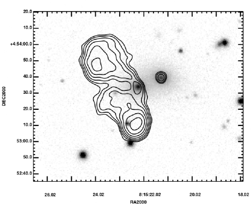
5mm normal

Figure 1: RC J0815+0453. A group of two radio sources. Each source is identified with an elliptical galaxy. The isophotes from the FIRST survey are superimposed on the corresponding r-filter image of the SDSS survey.

Radio sources with asymmetric structure—the so-called ‘‘winged’’ or ‘‘X-shaped’’ sources—constitute a small and interesting population of radio galaxies Cheung . In addition to the common pair of radio components, these objects have a pair of low surface brightness emitting regions, which form the wings or have an X-like shape. This shape is believed to be a result of plasma outflow from hot-spot regions into the inhomogeneous medium surrounding the radio source Leahy . Another explanation associates the unusual structure of the source with the fact that low-brightness regions may be residual phenomena of the rapid change of the rotational orientation of the system with a supermassive black hole (SMBH) and an accretion disk that occurred because of a recent merger of a double SMBH Dennett . X-shaped sources are of interest as systems associated with double black holes Komossa and recurrent phases of the activity of the radio source in the host galaxy Liu . We computed the number of radio sources with a close to ‘‘winged’’ or ‘‘X-shaped’’ structure. Such sources make up for about 4% of all the sources considered.

There are groups consisting of several sources and there are pairs located within 1-1.5 arcmin of each other. We found them to make up for about 7% of all the cases. Figure 1 shows an interesting example of a pair consisting of a double and a faint point radio source identified with two elliptical galaxies.

The results of the identification of radio sources with the VLSS, TXS, NVSS, FIRST, and GB6 surveys, the angular sizes, morphology, and spectral indices can be found in the electronic table available at http://www.sao.ru/hq/zhe/RCriResInn.html. One can also find there a description of the columns and contour maps of RC radio sources based on images of the FIRST survey.

4 THE 74–4850 MHZ SPECTRA OF RADIO SOURCES

The completeness of the RC catalog in the central part of the ‘‘Cold’’ survey is close to unity for radio sources with flux densities $S_{3.9\,GHz}$> 15 mJy Soboleva . This region includes the $10\hbox{${}^{\prime}$}$ wide declination strip centered on the declination of the SS 433 source at the epoch of the survey. Figure 2 shows the distribution of the flux densities of radio sources. The sharp decrease for faint sources starts at $S_{3.9\,GHz}$< 11–12 mJy. The catalog lists all objects with flux densities $S_{3.9\,GHz}\geq 30$ mJy in the 20^′ strip without exception. When composing two flux limited samples we took into account the declination difference between SS 433 and the radio-source coordinates refined using NVSS and precessed for the epoch of observations (15.04.1980), as well as the flux density refined using the corrected $\Delta H$ and the computed directional diagram of the telescope for the elevation of $H=51\hbox{${}^{\circ}$}$. The first complete sample includes sources with elevation differed from that of the center of the directional diagram by no more than $\Delta H\leq|5\hbox{${}^{\prime}$}|$ and with fluxes equal to or greater than $S_{3.9\,GHz}\geq$11 mJy (a total of 130 objects). The sample covers an area of about 21 $\square\hbox{${}^{\circ}$}$ The second sample consists of the sources with $\Delta H\leq|10\hbox{${}^{\prime}$}|$ and $S_{3.9\,GHz}\geq$ 30 mJy (a total of 117 objects covering an area of about 41 $\square\hbox{${}^{\circ}$}$). The samples partly overlap, because 47% of the sources of the second sample belong to the first sample. Hereafter for the sake of brevity we refer to the first and second samples as 1S and 2S, respectively.

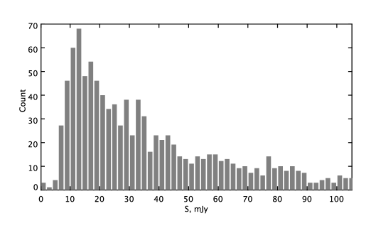
5mm normal

Figure 2: Distribution of the 3.9 GHz flux densities of the RC catalog sources (sources brighter than 105 mJy are not plotted). The number of sources decreases sharply at flux densities <12 mJy.

5mm flushleft
Spectrum Sample Fraction of the sample $N_{obj}$ $LAS_{median}$ $S_{1.4\;GHz}$ $S_{3.9\;GHz}$ $S_{4.85\;GHz}$ $\alpha_{median}$ (%) (^′′) (mJy) (mJy) (mJy) I 1S 10 13 2.33 12.1 14 20 -0.32 2S 6 7 2.33 34.3 68 51 -0.32 F 1S 27 35 2.34 39.1 22 28 0.31 2S 22 26 2.27 74.2 45 46 0.25 S 1S 54 70 10.6 82.3 31 33 0.76 2S 56 65 10.26 146.5 57 59 0.76 U 1S 9 12 17.1 94.5 31 22 1.17 2S 16 19 17.1 146.1 69 39 1.12

Table 3: Distribution of the types of the spectra (of the spectral index $\alpha_{1.4-4.85\;GHz}$) of the sources in the 1S ($\Delta H\leq|5\hbox{${}^{\prime}$}|$; $S_{3.9\;GHz}\geq$11 mJy) and 2S ($\Delta H\leq|10\hbox{${}^{\prime}$}|$; $S_{3.9\;GHz}\geq$30 mJy) samples

We used the images of the GB6 survey to estimate the 4.85 GHz fluxes for the sources of the sample that were absent in the GB6 catalog. For this, we compared the peak intensities in the region of the radio source studied and of the neighboring sources listed in the GB6 catalog. Note that for the GB6 catalog the 5$\sigma$ detection limit for radio sources located at $\delta\sim+5\hbox{${}^{\circ}$}$ is about 28 mJy in the right-ascension intervals $8^{h}<\alpha_{2000.0}<12^{h}$ and $14^{h}40^{m}<\alpha_{2000.0}<16^{h}30^{m}$ and about 37 mJy in the right-ascension interval $12^{h}<\alpha_{2000.0}<14^{h}40^{m}$ Gregory . Out from the 130 sources of the 1S sample 51 source was identified with the GB6 catalog and for the remaining 79 sources we give the flux density estimates inferred from the images of the GB6 survey. For the 2S sample the corresponding numbers are equal to 85 and 32, respectively.

We subdivided all sources into four groups in accordance to their spectral index $\alpha_{1.4-4.85\,GHz}$ (see Table 3):

• inverse (I), $\alpha<-0.1$;

• flat (F), $-0.1\leq\alpha<0.5$;

• steep (S), $0.5\leq\alpha<1$;

• ultrasteep (U), $\alpha\geq 1$.

The median flux density of the sources is equal to $S^{median}_{3.9\,GHz}$=26 mJy and $S^{median}_{3.9\,GHz}$=57 mJy for the first (1S) and second (2S) samples, respectively. A comparison of the spectral indices of the radio sources shows that the number of sources with inverse and flat spectra slightly increases and that of the sources with steep and ultrasteep spectra decreases (see Table 3 and Fig. 3).

The sources with flat and inverse spectra of the 1S and 2S samples proved to be more compact in terms of angular sizes (see Table 3) than sources with steep and ultrasteep spectra.

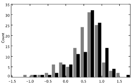
5mm normal

Figure 3: Distribution of spectral indices $\alpha_{1.4\,GHz-4.85\,GHz}$ for sources from the central part of the ‘‘Cold’’ survey. The gray and black histograms correspond to the sources of the 1S ($\Delta H\leq|5\hbox{${}^{\prime}$}|$; $S_{3.9\;GHz}\geq$11 mJy) and 2S ($\Delta H\leq|10\hbox{${}^{\prime}$}|$; $S_{3.9\;GHz}\geq$30 mJy) samples, respectively. The 1S sample, which includes sources with smaller 3.9 GHz flux densities compared to the 2S sample contains more flat and inverse spectra than the 2S sample.

For the 143 sources identified in three or four catalogs (VLSS, TXS, NVSS, and GB6) additional flux density information is available, which allows the behavior of their spectra to be studied in the frequency interval 74–4850 MHz. We estimated the flux densities of objects with no data given in the VLSS or GB6 catalog by comparing the peak value in the region of the radio source with the peak values for the neighboring sources listed in the corresponding catalogs. We set the flux densities of the sources absent in the TXS catalog equal to the 150-mJy sensitivity limit of the catalog. We then computed the two-frequency spectral indices $\alpha_{74-365\;MHz}$, $\alpha_{365\;MHz-1.4\;GHz}$, and $\alpha_{1.4-4.85\;GHz}$. We found the fractions of sources with inverse, flat, steep, and ultrasteep spectral indices $\alpha_{74-365\;MHz}$ proved to be equal to 10%, 38%, 46%, and 6%, respectively.The sources of the first group proved to be more compact ($LAS_{median}=1.02\hbox{${}^{\prime\prime}$}$) than other sources.

In each group we analyzed how the form of the spectrum varies from low to higher frequencies by fitting the spectrum to a parabola using the spg procedure of the standard FADPS reduction system of the first feeder of RATAN-600 Verkhodanov1 . We use symbols I, F, S, and U to denote the corresponding regions of the spectrum as we pass from one portion to another. We obtained the following results (see Table 4):

• Sources with $\alpha_{74-365\;MHz}$<-0.1 have two types of spectra: one group has a steep spectrum at 1.4 GHz, which becomes steep (IFS) or ultrasteep (IFU) by 4.85 GHz, and the second group has ultrasteep spectra at 1.4 GHz.

• Sources with flat spectra can be subdivided into the following three groups:

• The spectra of most of the sources (29% of all sources) become steeper with increasing frequency (FS, FU);

• A small number of sources maintain flat spectrum in the frequency interval considered (F) or become inverse at high frequencies (FI);

• The third group includes sources with spectra $\alpha_{365\;MHz-1.4\;GHz}$>0.5, and flatten out by 4.85 GHz (FSF).

• Sources with steep spectra can also subdivided into three groups:

• Most of the sources (34%) have steep spectra whose spectral indices remain unchanged ($\alpha>0.5$) as one passes from one spectral interval to another. We fit Sc SU to a parabola. At high frequencies the spectra of SU sources become ultrasteep and those of Sc sources remain steep);

• A small number of sources with flattened or inverse spectra at 4.85 GHz (SF—3.5%, SI—1.5%);

• The third group—transition from a steep to a flat spectrum, and then back to a steep spectrum (SFS).

• The small group of sources with ultrasteep spectra in the frequency interval 74–365 MHz can be subdivided into the following two sub groups:

• one of the subgroups maintains its steep spectrum at higher frequencies, but its slope is smaller than the initial slope (US);

• the spectra of the objects of the second subgroup becomes flat (UF) or even inverse (UFI).

0mm flushleft
$\alpha_{74-365\;MHz}$ Form of the spectrum Fraction in the sample Number of objects $LAS_{median}$ (%) (^′′) I IFS 3 4 0.91 15 (10%) IFU 2 3 1.35 IU 5 8 1.02 F 4 6 11.0 F FS 15 22 5.25 55 (38%) FU 14 20 7.02 FI 1.5 2 1.40 FSF 3.5 5 4.83 S 11 15 13.6 S Sc 13 19 20.9 65 (46%) SU 10 14 14.0 SF 3.5 5 4.57 SI 1.5 2 5.9 SFS 7 10 51.6 U US 2 3 53.0 8 (6%) UF 3 4 16.5 UFI 1 1 0.76

Table 4: Variation of the spectral indices $\alpha_{74-365\;MHz}$, $\alpha_{365\;MHz-1.4\;GHz}$, and $\alpha_{1.4-4.85\;GHz}$ for 143 RC sources according to the data of the VLSS, TXS, NVSS, and GB6 surveys

5 CONCLUSIONS

We cross identified 432 radio sources of the RC catalog located within the region of intersection of the SDSS and FIRST surveys of the FIRST, NVSS, TXS, VLSS, and GB6 catalogs. In our statistical study and optical identifications we use the sources (about 75% of all sources) identified with the NVSS and/or FIRST catalogs. Most of the remaining RC objects (about 25% of all sources) are either false or blends of two or more real objects whose individual properties are difficult to determine from observations of the ‘‘Cold’’ survey.

We use the data of the FIRST survey to compute the number of components (entries of the FIRST catalog) for the sources studied. We found that single-component sources and sources with two or more components account for about 56% and more than 44% of the entire sample, respectively.

This result is inconsistent with the results of automatic cross identification between the FIRST survey on the one hand and SDSS and APM surveys on the other hand McMahon1 ; Ivezic , and the estimate (84%) of the fraction of single-component sources in the FIRST survey as reported by Cress et al. Cress due to brighter flux density sample. The fraction of radio sources that are difficult to automatically identify is about 15% for a high angular resolution survey (such as FIRST).

The completeness of the RC catalog is close to unity in the central part of the ‘‘Cold’’ for radio sources with flux densities $S_{3.9\,GHz}>15$ mJy, and decreases toward the strip boundaries Soboleva . That is why to compare the parameters of radio sources, two complete samples in the central part of the survey are considered. The first sample includes the sources with elevation deviates from the directional diagram of the telescope by less than $\Delta H\leq|5\hbox{${}^{\prime}$}|$ and with flux densities that are greater than or equal to $S_{3.9\,GHz}\geq 11$ mJy. The sample covers an area of about 21 $\square\hbox{${}^{\circ}$}$. The second sample includes the sources with $\Delta H\leq|10\hbox{${}^{\prime}$}|$ and $S_{3.9\,GHz}>29$ mJy (the total area is equal to about 41 $\square\hbox{${}^{\circ}$}$). The first (1S) and second (2S) samples contain a total of 130 and 117 objects, respectively. The two samples partially overlap.

We computed the spectral index $\alpha_{1.4-4.85\,GHz}$ for all sources in both samples and then subdivided these sources into the following four groups:

• inverse (I), $\alpha<-0.1$;

• flat (F), $0.1\leq\alpha<0.5$;

• steep (S), $0.5\leq\alpha<1$;

• ultrasteep (U), $\alpha\geq 1$.

A comparison of the two samples, with one of them being deeper than the other in flux density terms, shows that the number of sources with inverse and flat spectra in the frequency interval 1.4–4.85 GHz slightly increases with decreasing flux density, i.e., the fraction of such sources is equal to 37% and 28% in the first and second samples, respectively. The number of sources with steep and ultrasteep spectra increases—the fraction of such sources is equal to 63% and 72% in the 1S and 2S samples, respectively. The distribution of the spectral indices $\alpha_{1.4-4.85\,GHz}$ of the sources in the 2S sample is shifted toward steeper indices with respect to the corresponding distribution for the 1S sample.

Sources with flat and inverse spectra in the 1S and 2S samples proved to be more compact in terms of angular sizes compared to sources with steep and ultrasteep spectra.

For sources identified in the VLSS, TXS, NVSS, and GB6 catalogs additional flux density information is available allowing the behavior of their radio spectra to be compared in the frequency interval 74–4850 MHz. We computed the two-frequency spectral indices $\alpha_{74-365\;MHz}$, $\alpha_{365\;MHz-1.4\;GHz}$, and $\alpha_{1.4-4.85\;GHz}$ and fitted the spectra to a parabolic function. We could identify eight groups of spectra and found the spectra of most of the sources (about 60%) to be flat or steep ones in the frequency interval 74–365 MHz and to remain or become steep at high frequencies. About 10% of the sources have S-shaped spectra (the fractions of FSF and SFS objects are equal to about 3% and 7%, respectively). There are few (less than 3%) sources with a transition from a flat to a steep or inverse spectrum. Radio sources with inverse spectrum in one of the portions of the frequency interval considered proved to be compact in terms of angular size.

We paid special attention to the morphological classification of radio sources from the subsequent optical identification point of view. We classify radio sources in accordance with a morphological scheme based on the comparison of the structure of the radio source and the position of the optical object. We classified 39% of the objects as belonging to the point type (C core); 40% of the sources as double sources (D—double-lobe, DC—double-core-lobe, DD—double-double), and about 20% of all objects as triple, multicomponent, and other types of sources.

For the RC radio sources identified with SDSS, USNO, and 2MASS catalogs we found optical identifications, which we will report in a separate paper.

- (1) J.J. Condon, et al., Astronom. J.115, 1693 (1998).
- (2) R.H. Becker, et al., Astrophys. J. 475, 479 (1997).
- (3) R.G. McMahon, et al., Astrophys. J. Suppl.143, 1 (2002).
- (4) R.G. McMahon, et al., VizieR On-line Data Catalog: I267 (Cambridge, CB3 OHA, UK, Institute of Astronomy, 2000)
- (5) G.O. Abell, Astronomical Society of the Pacific Leaflets 8, 121 (1959).
- (6) C. Stoungton, et al., Astronom. J. 123, 485 (2002).
- (7) . Ivezi, et al., Astronom. J.124, 2364 (2002).
- (8) A.B. Berlin et al., AstL 7, 290 (1981).
- (9) A.B. Berlin et al., AstL 9, 211 (1983).
- (10) Yu.N. Pariiskij, et al., Astronom. and Astrophys. Suppl. Ser.87, 1 (1991).
- (11) Yu.N. Pariiskij, et al., Astronom. and Astrophys. Suppl. Ser.96, 583 (1992).
- (12) O.V. Verkhodanov, et al., Baltic Astronomy 9, 604 (2000).
- (13) A.S. Cohen, et al., Astronomische Nachrichten 327, 262 (2006).
- (14) A.S. Cohen, et al., Astronom. J.134, 1245 (2007).
- (15) J.N. Douglas, et al., Astronom. J.111, 1945 (1996).
- (16) P.C. Gregory, et al., Astrophys. J. Suppl.103, 427 (1996).
- (17) J.K. Adelman-McCarthy, et al., Astrophys. J. Suppl.172, 634 (2007).
- (18) N.A. Esepkina et al.,Radiotekhnika i Electronika 6, No 12, 1947 (1961).
- (19) E.K. Majorova and S.N. Trishkin, BSAO 54, 89 (2002).
- (20) R. Williams, et al., http://www.ivoa.net/ Documents/latest/ConeSearch.html.
- (21) B. Vollmer, et al., Astronomy and Astrophysics 436, 757 (2005).
- (22) F. Ochsenbein, et al., in Proceedings of the ADASS XIV, Pasadena, USA, 2004), Eds.: P. Shopbell, M. Britton, and R. Ebert (ASP Conf. Series, 347, 2005), p.193.
- (23) F. Ochsenbein et al., Astronom. and Astrophys. Suppl. Ser.143, 23 (2000).
- (24) M.B. Taylor, in Proceedings of the ADASS XIV, Pasadena, USA, 2004), Eds.: P. Shopbell, M. Britton, and R. Ebert (ASP Conf. Series, 347, 2005), p.29.
- (25) N.S. Soboleva, Abstract of the Doctoral Dissertation in Math. and Physics, (SAO RAS, Nizhnij Arkhyz, 1992) 47p
- (26) J. Dennett-Thorpe, et al., Monthly Notices Roy. Astronom. Soc.330, 609 (2002).
- (27) S. Komossa, Proceedings of the International Conference The Astrophysics of Gravitational Wave Sources (AIP Conf. Proc., 686, 2003), p.161.
- (28) A.I. Kopylov, http://www.sao.ru/hq/zhe/ATLAS.
- (29) FIRST cutout service, http://www.mrao.cam.ac.uk/surveys/FIRST/.
- (30) C.M. Cress et al., Astronom. J. 473, 7 (1996).
- (31) C.R. Lawrence et al., Astrophys. J. Suppl. 61, 105 (1986).
- (32) C.C Cheung, Astronom. J.133, 2097 (2007).
- (33) J.P. Leahy, A.G. Williams, Monthly Notices Roy. Astronom. Soc.210, 92 (1984).
- (34) J. Dennett-Thorpe et al., Monthly Notices Roy. Astronom. Soc.330, 609 (2002).
- (35) F.K. Liu, Monthly Notices Roy. Astronom. Soc.347, 1357 (2004).
- (36) O.V. Verkhodanov, in Proceedings of the ADASS VI, Pasadena, USA, 1996), Eds.: G. Hunt and H.E. Pyne (ASP Conf. Series, 125, 1997), p.47.