A view of Neural Networks as dynamical systems.

Abstract

We present some recent investigations resulting from the modelling of neural networks as dynamical systems, and dealing with the following questions, adressed in the context of specific models.

1. Characterizing the collective dynamics;

2. Statistical analysis of spikes trains;

3. Interplay between dynamics and network structure;

4. Effects of synaptic plasticity.

The study of neural networks is certainly a prominent example of interdisciplinary research field. From biologists, neurophysiologists, pharmacologists, to mathematicians, theoretical physicists, including engineers, computer scientists, robot designers, a lot of people with distinct motivations and questions are interacting. With maybe a common “Graal”: to understand one day how brain is working. At the present stage, and though significant progresses are made regularly, this promised day is however still in a far future. But, beyond the comprehension of brain or even of simpler neural systems in less evolved animals, there is also the desire to exhibit general mechanisms or principles that could be applied to such artificial systems as computers, robots, or “cyborgs” (we think of the promising research field of brain-control of artificial prostheses, see for example the web page http://www-sop.inria.fr/demar/index_fr.shtml). Again, there are many way of tracking these principles or mechanisms.

One possible strategy is to propose mathematical models of neural activity, at different space and time scales, depending on the type of phenomenon under consideration. However, beyond the mere proposal of new models, which can rapidly results in a plethora, there is also a need to understand some fundamental keys ruling the behaviour of neural networks, and, from this, to extract new ideas that can be tested in real experiments. Therefore, there is a need to make a thorough analysis of these models. This can be done by numerical investigations, with, very often, the need of inventing clever algorithms to fight the hard problem of simulating, in a reasonable time, and with a reasonable accuracy, the tremendous number of degree of freedom and the even larger number of parameters that neural networks have. A complementary issue relies in developing a mathematical analysis, whenever possible.

In this spirit, we present in this paper some recent investigations from the authors and his collaborators, resulting from the modelling of neural networks as dynamical systems. We warn the reader that this paper does not intend to be exhaustive and we shall only briefly mention many works which certainly would have deserved a longer presentation in a more extensive review: the works by Ermentrout and Kopell on phase response theory [67], van Vreeswijk, Sompolinsky and collaborators [177, 178, 176, 175], [120], Brunel [34, 32, 71, 72, 33, 144], and many others on neural activity, theory of synchronization and spike patterns by Seung [181], Bressloff and Coombes [28, 27, 29] Timme [169, 11, 126, 101], Jin [87], Diesmann [63] are only a few examples of these omissions.

Beyond the presentation of those results there is also the willing of raising interesting questions emerging from this point of view. After a short presentation of neural networks, and how they can be indeed modeled as dynamical systems (section 1), we list $4$ of these questions, and address them in specific models.

• Characterizing the collective dynamics of neural networks models. When considering neural networks as dynamical systems, a first, natural issue is to ask about the (generic) dynamics exhibited by the system when control parameters vary. This is discussed in section 2.

• Statistical analysis of spikes trains. Neurons respond to excitations or stimuli by finite sequences of spikes (spike trains). Characterizing spike trains statistics is a crucial issue in neuroscience. We approach this question considering simple models. This is discussed in section 3.

• Interplay between dynamics and synaptic network structure. Neural network are highly dynamical object and their behavior is the result of a complex interplay between the neurons dynamics and the synaptic network structure. In this context, we discuss how the mere analysis of synaptic network structure may not be sufficient to analyse such effects as the propagation of a signal inside the network. We also present new tools based on linear response theory [151], useful to analysing this interwoven evolution. This is discussed in section 4.

• Effects of synaptic plasticity. Synapses evolve according to neurons activity. Addressing the effect of synaptic plasticity in neural networks where dynamics is emerging from collective effects and where spikes statistics are constrained by this dynamics seems to be of central importance. We present recent results in this context. This is discussed in section 5.

Obviously, the scope of this paper is not to address these questions in a general context. Instead, we choose to present simple examples, that one may consider as rather “academic”, for which one can go relatively deep, with the idea that such investigations may reveal useful, when transposed to “realistic” neural networks.

1 Neural Networks as dynamical systems

1.1 From biological neurons and synapses $\dots$

A neuron is an excitable cell. Its activity is manifested by local variations (in space and time) of its membrane potential, called “action potentials” or “spikes”. These variations are due to an exchange of ions species (basically $Na^{+}$,$K^{+}$,$Cl^{-}$) which move, through the membrane, from the region of highest concentration (outside for $Na^{+}$, inside for $K^{+}$) to the region of lowest concentration. This motion does not occur spontaneously. It requires the opening/closing of specific gates in specific ionic channels. The probability that a gate is open depends on the local membrane potential, whose variations can be elicited by local excitations, induced by external currents, or coming from neighbours pieces of membrane (spike propagation). Neurons have a spatial structure, depicted in fig 1, and spikes propagates along this structure, from dendrites to soma, and from soma to synapses, along the axon.

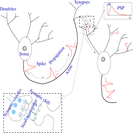
Figure 1: Sketch of the neuron structure.

The response of a given neuron to excitations has a wide variability. This variability is not manifested by the shape of the action potential, which is relatively constant for a given neuron. Instead, it is revealed by the various sequences of spikes a neuron is able to emit. Depending on the excitation, the response can be an isolated spike, a periodic spike train, a burst, etc… About twenty different spike trains forms are classified in the literature [99].

Neurons are connected together. When a spike train is emitted from the soma toward the synapses, via the axon, it eventually reaches the synaptic vesicles. Here, a local variation of the membrane potential triggers the release of a neurotransmitter into the synaptic cleft. This neurotransmitter reaches by diffusion the post-synaptic receptors, located on the dendritic spines, and generates a post-synaptic potential (PSP). Contrarily to spikes, PSP have an amplitude which depends on the amplitude of the excitation and on the synaptic efficacy. Efficacy evolves according to various mechanisms depending on the activity of pre- and post-synaptic neurons. Depending on the pre-synaptic neuron and the neurotransmitter used by this neuron, the PSP can be either positive or negative. In the first case the pre-synaptic neuron and its synaptic connections are called excitatory. Spikes coming from pre-synaptic neuron increase the membrane potential of the post-synaptic neuron which is more keen on generating spike trains. Or PSP can be negative, corresponding to an inhibitory pre-synaptic neuron.

Typically, a neuron is connected to many pre-synaptic neurons and receives therefore many excitatory or inhibitory signals. The cumulative effects of these signals eventually generate a response of this neuron’s soma that propagates along the axon up to the synaptic tree, then acting on other neurons, and so on.

From this short description, we can make the following summary.

• Neurons are connected to each others in a synaptic network with causal (action/reaction) interactions.

• Signals exchanged by neurons are spike trains. Spike trains coming from pre-synaptic neurons generate a spike train response of the post-synaptic neuron which propagates to other neurons.

• Spike trains have a wide variability which generates an overwhelming repertoire of collective dynamical responses.

As an additional level of complexity the structure of the network constituted by synaptic connections can also have a wide range of forms, with multiple layers, different species of neurons, etc. Also, a very salient property is the capacity that synapses have to evolve and adapt, according to plasticity mechanisms. Synaptic plasticity occurs at many levels of organisation and time scales in the nervous system [20]. It is of course involved in memory and learning mechanisms, but it also alters excitability of brain area and regulates behavioural states (e.g. transition between sleep and wakeful activity). On experimental grounds, synaptic changes can be induced by specific simulations conditions defined through the firing frequency of pre- and post-synaptic neurons [23, 64], the membrane potential of the post-synaptic neuron [10], spike timing [119, 124, 19] (see [123] for a review). Different mechanisms have been exhibited from the Hebbian’s ones [90] to Long Term Potentiation (LTP) and Long Term Depression (LTD), and more recently to Spike Time Dependent Plasticity (STDP) [124, 19] (see [60, 77, 52] for a review).

1.2 $\dots$ to models

Regarding the overwhelming richness of behaviors that neuronal networks are able to display, the theoretical (mathematical or numerical) analysis of these systems is at a rather early stage. Nevertheless, some significant breakthrough have been made within the last 50 years, as we shall see in a few examples. For this, a preliminary modeling/simplification strategy is necessary, that we summarize as follows.

1.2.1 Fix a model of neuron

This essentially means: fix an equation or a set of equations describing the evolution of neuron’s membrane potential, plus, possibly, additional variables (such as the probability of opening/closing ionic gates in Hodgkin-Huxley’s like models [94]). This choice can be guided by different and, often, mutually incompatible constraints.

• Biological plausibility.

• Mathematical tractability.

• Numerical efficiency.

Regarding the first aspect one may also only focus on a few biological features. Do we want a model that reproduces accurately spike shape, or do we simply want to reproduce the variability in spike trains responses whereas spike shape is neglected (e.g. represented by a “Dirac” peak) ? Do we want to focus on one specific characteristic of spike trains (probability that a neuron fires, probability that two neurons fire within a certain time delay….) ? Clearly, there is a large number of neuron models and, as usual, models depend on the questions that you ask. Here are a few examples.

Hodgkin-Huxley model.

This model, dating back to 1952 [94], is still one of the best description of neuron spike generation and propagation. Thus, it is very good from the point of view of biological plausibility. Unfortunately, its mathematical analysis has not been completed yet and it is computational time consuming. In this model, the dynamics of a piece of membrane with capacity $C_{m}$ and potential $V$ is given by:

$$C_{m}\frac{dV}{dt} = -g_{Na}m^{3}h(V-E_{Na})-g_{K}n^{4}(V-E_{K})-g_{L}(V-E_{L})+I_{ext}$$ (1)

$$\frac{1}{\gamma(T)}\frac{dn}{dt} = \alpha_{n}(V)(1-n)-\beta_{n}(V)n=\frac{n^{\infty}(V)-n}{\tau_{n}(V)}$$ (2)

$$\frac{1}{\gamma(T)}\frac{dm}{dt} = \alpha_{m}(V)(1-m)-\beta_{m}(V)m=\frac{m^{\infty}(V)-m}{\tau_{m}(V)}$$ (3)

$$\frac{1}{\gamma(T)}\frac{dh}{dt} = \alpha_{h}(V)(1-h)-\beta_{h}(V)h=\frac{h^{\infty}(V)-h}{\tau_{h}(V)}$$ (4)

where $m,h,n$ are additional variables, describing the ionic channels activity (see [58, 76, 92, 111, 116, 134]). $E_{Na},E_{K},E_{L}$ are respectively the Nernst potentials of $Na^{+},K^{+}$ ions and additional ionic species (like $Cl^{-}$) grouped together in a leak potential $E_{L}$. $g_{N}a$,$g_{K}$, $g_{L}$ are the corresponding conductances. $\gamma(T)$ is a temperature dependent time scale (equal to $1$ at $6.3^{o}$C). $\alpha,\beta$ are transitions rates in the masters equations (2,3,4) used to model the transition open/close of ionic channels. Though the complete mathematical analysis of this model has not been performed yet, important results can be found in [58, 111, 84, 85].

Fitzhugh-Nagumo model

One can reduce the Hodgkin-Huxley equations in order to obtain an analytically tractable model. In this spirit Fitzhugh [70] and independently Nagumo, Arimoto & Yoshizawa [133], considered reductions of the Hodgkin-Huxley model and introduced an analytically tractable two variables model

$$\begin{array}[]{lll}\epsilon\frac{dv}{dt}&=&f_{\lambda}(v,w),\\ \frac{dw}{dt}&=&g_{\lambda}(v,w),\end{array}$$

where $\epsilon$ is a small parameter. The index $\lambda$ refers to the control parameters of the system. In the FitzHugh-Nagumo model $f_{\lambda}(v,w)=v-v^{3}-w+I$ is a cubic polynomial in $v$ and is linear in $w$, while $g_{\lambda}(v,w)=(v-a-bw)$. The parameters $\lambda=(a,b,I)$ are deduced from the physiological characteristics of the neuron.

Integrate and Fire models

Here, one fixes a real number $\theta$, called the firing threshold of the neuron, such that if $V_{k}(t)\geq\theta$ then neuron membrane potential is reset instantaneously to some constant reset value $V_{reset}$ and a spike is emitted toward post-synaptic neurons. Below the threshold, $V_{k}<\theta$, neuron $k$’s dynamics is driven by an equation of form:

$$C_{k}\frac{dV_{k}}{dt}+g_{k}V_{k}=i_{k},$$ (5)

where $C_{k}$ is the membrane capacity of neuron $k$, $g_{k}$ its conductance and $i_{k}$ a current, including various term, depending on modeling choices (external current, ionic current, adaptation current).

In its simplest form equation (5) reads:

$$\frac{dV_{k}}{dt}=-\frac{V_{k}}{\tau_{k}}+\frac{i_{k}}{C_{k}},$$ (6)

where $g_{k}$ is a constant, and $\tau_{k}=\frac{g_{k}}{C_{k}}$ is the characteristic time for membrane potential decay, when no current is present. This model has been introduced in [118]. More generally, conductances and currents depend on the previous firing times of the pre-synaptic neurons [149] (see section 2.2 for an example).

Discrete time models

In many papers, researchers use sooner or later numerical simulations to guess or validate original results. Most often this corresponds to a time discretisation with standard schemes like Euler, or Runge-Kutta. Even when seeking more elaborated schemes such as event based integrations schemes [31, 146], which in principle allows one to handle continuous time, there is in fact a minimal time scale, due to numerical round-off error, below which the numerical scheme is not usable anymore. On more fundamental grounds, in all models presented above including Hodgkin-Huxley, there is a minimal time scale imposed by Physics. Thus, although the mathematical definition of $\frac{d}{dt}$ assumes a limit $dt\to 0$, there is a time scale below which the ordinary differential equations lose their meaning. Actually, the mere notion of “membrane potential” already assumes an average over microscopic time and space scales. Another reason justifying time discretisation in models is the use of “raster plot” to characterize neurons activity.

Raster plots

A raster plot is a graph where the activity of a neuron is represented by a mere vertical bar each “time” this neuron emits a spike. When focusing on spiking neurons models, spikes are often characterized by their “time” of occurrence. Except for IF models, where the notion of “instantaneous” firing and reset leads to nice pathologies, a spike has some duration and spike time has some uncertainty $\delta$. Therefore, the statement “neuron $i$ fires at time $t$” must be understood as “neuron $i$ fires at time $t$ within a precision $\delta>0$”. Moreover, a neuron cannot fire more than once within a time period $r$ called “refractory period”. Therefore, one can fix a positive time scale $\delta>0$ which can be mathematically arbitrary small, such that (i) a neuron can fire at most once between $[t,t+\delta[$ (i.e. $\delta<<r$, the refractory period); (ii) $dt<<\delta$, so that we can keep the continuous time evolution of membrane potentials, taking into account time scales smaller than $\delta$, and integrating membrane potential dynamics on the intervals $[t,t+\delta[$; (iii) the spike time is known within a precision $\delta$ (see [114] for an interesting discussion on this approach).

At this stage let us introduce a concept/notation used throughout this paper. One can associate to each neuron $k$ a variable $\omega_{k}(t)=1$ if neuron $k$ fires between $[t,t+\delta[$ and $\omega_{k}(t)=0$ otherwise. A “spiking pattern” is a vector $\boldsymbol{\omega}(t)\stackrel{{\scriptstyle\rm def}}{{=}}\left[\omega_{k}(t)\right]_{k=1}^{N}$ which tells us which neurons are firing at time $t$. A “raster plot” is a sequence $\omega\stackrel{{\scriptstyle\rm def}}{{=}}\left\{\boldsymbol{\omega}(t)\right\}_{t=0}^{+\infty}$, of spiking patterns. We denote $\left[\omega\right]_{0,t}=\left\{\boldsymbol{\omega}(s)\right\}_{s=0}^{t}$, the raster plot from time $0$ to time $t$.

1.2.2 Fix a model of synapse

Voltage- and activity-based models

A single action potential from a pre-synaptic neuron $j$ is seen as a post-synaptic potential by a post-synaptic neuron $i$ (see Fig. 1). The conductance time-course after the arrival of a post-synaptic potential is typically given by a function $\alpha_{ij}(t-s)$ where $s$ is the time of the spike hitting the synapse and $t$ the time after the spike. (We neglect here the delays due to the distance travelled down the axon by the spikes). In voltage-based models one assumes that the post-synaptic potential has the same shape no matter which pre-synaptic population caused it, the sign and amplitude may vary though [66]. This leads to the relation:

$$\alpha_{ij}(t)=W_{ij}\alpha_{i}(t),$$

where $\alpha_{i}$ represents the unweighted shape (called a $\alpha$-shape) of the post-synaptic potentials. Known examples of $\alpha$-shapes are $\alpha_{i}(t)=K_{i}e^{-t/{\tau_{i}}}H(t)$ or $\alpha_{i}(t)=K_{i}te^{-t/{\tau_{i}}}H(t)$ where $H$ is the Heaviside function. More generally this is a polynomial in $t$ and this is the Green function of a linear differential equation of order $k$:

$$\sum_{l=0}^{k}a^{(l)}_{i}\frac{d^{l}\alpha_{i}}{dt^{l}}(t)=\delta(t).$$ (7)

$W_{ij}$ is the strength of the post-synaptic potentials elicited by neuron $j$ on neuron $i$ (synaptic efficacy or “synaptic weight”).

In activity-based models the shape of a PSP depends only on the nature of the pre-synaptic cell, that is [66]:

$$\alpha_{ij}(t)=W_{ij}\alpha_{j}(t).$$

Assuming that the post-synaptic potentials sum linearly, the average membrane potential of neuron $i$ is:

$$V_{i}(t)=\sum_{j,n}\alpha_{ij}(t-t_{j}^{(n)}),$$ (8)

where the sum is taken over the arrival times $t_{j}^{(n)}\leq t$ of the spikes produced by the neurons $j$.

Synaptic plasticity.

Most often, the mechanisms involved in synaptic plasticity have been revealed by simulation performed in isolated neurons in in vitro conditions. Extrapolating the action of these mechanisms to in vivo neural networks requires both a bottom-up and top-down approach. This issue is tackled, on theoretical grounds, by inferring “synaptic updates rules” or “learning rules” from biological observations [179, 20, 128] (see [60, 77, 52] for a review) and extrapolating, by theoretical or numerical investigations, what are the effects of such synaptic rule on such neural network model. This approach relies on the belief that there are “canonical neural models” and “canonical plasticity rules” capturing the most essential features of biology. When considering synaptic adaptation, one proposes evolution rules for the $\alpha_{ij}$ profiles. Most often, the mere evolution of the $W_{ij}$’s are considered. Here are a few typical examples.

Generic synaptic update

Synaptic plasticity corresponds to the evolution of synaptic efficacy which evolve in time according to the spikes emitted by the pre- and post- synaptic neuron. In other words, the variation of $W_{ij}$ at time $t$ is a function of the spiking sequences of neurons $i$ and $j$ from time $t-T_{s}$ to time $t$, where $T_{s}$ is time scale characterizing the width of the spike trains influencing the synaptic change. In its more general form synapse update reads:

$$\delta Wij=g\left(W_{ij}(t),\left\{t_{i}^{(l)}\right\}_{t},\left\{t_{j}^{(n)}\right\}_{t}\right),\ t>T_{s},$$

where $\left\{t_{i}^{(l)}\right\}_{t}$, ($\left\{t_{j}^{(n)}\right\}_{t}$) are the lists of spikes times emitted by the pre-synaptic neuron $i$, (the post-synaptic neuron $j$), up to time $t$. Thus, synaptic adaptation results from an integration of spikes over the time scale $T_{s}$.

With the concept of “raster plot” introduced at the end of section 1.2.2, we may also write:

$$\delta Wij=g\left(W_{ij}(t),\left[\omega_{i}\right]_{t-T_{s},t},\left[\omega_{j}\right]_{t-T_{s},t}\right),\ t>T_{s}.$$ (9)

Let us now give a few examples of synaptic adaptation “rules”.

Hebbian learning

In this case, synapses changes depend on the firing rate of neuron $i$,$j$. A typical example corresponds to

$$g_{ij}(W_{ij},\left[\omega_{i}\right]_{t-T_{s},t},\left[\omega_{j}\right]_{t-T_{s},t})=\frac{1}{T_{s}}\sum_{s_{1},s_{2}=t-T_{s}}^{t}(\omega_{i}(s_{1})-r_{i}(s_{1}))(\omega_{j}(s_{2})-r_{j}(s_{2}),$$ (10)

(correlation rule [143]) where $r_{i}(t)=\frac{1}{T_{s}}\sum_{s=t-T_{s}}^{t}\omega_{i}(s)$ is the frequency rate of neuron $i$ in the raster plot $\omega$, computed in the time window $[t-T_{s},t]$.

Spike-Time Dependent Plasticity

as derived from Bi and Poo [19] provides the average amount of synaptic variation given the delay between the pre- and post-synaptic spike. Thus, “classical” STDP reads [77, 100]:

$$g\left(W_{ij},\left[\omega_{i}\right]_{t-T_{s},t},\left[\omega_{j}\right]_{t-T_{s},t}\right)=\sum_{s_{1},s_{2}=t-T_{s}}^{t}f(s_{1}-s_{2})\omega_{i}(s_{1})\omega_{j}(s_{2}),$$ (11)

with:

$$f(x)=\left\{\begin{array}[]{lll}A_{-}e^{\frac{x}{\tau_{-}}},\ x<0;\\ A_{+}e^{-\frac{x}{\tau_{+}}},\ x>0;\\ 0,\ x=0;\end{array}\right.$$ (12)

where $A_{-}<0$ and $A_{+}>0$. The shape of $f$ has been obtained from statistical extrapolations of experimental data. Hence STDP is based on a second order statistics (spikes correlations). There is, in this case, an evident time scale $T_{s}=\max(\tau_{-},\tau_{+})$, beyond which $f$ is essentially zero.

Many other examples can be found in the literature [100] .

1.2.3 Fix a synaptic graph structure

This point is closely related to the previous one. In particular, this structure can be fixed or evolve in time (synaptic plasticity). In this last case, there is a complex interaction between neuron dynamics and synapses dynamics. This structure can be guided from biological/anatomical data, or it can be random. In this last case, one is more interested in generic mathematical properties than by biological considerations. The intermediate case can also be considered as well: deterministic synaptic architecture with random fluctuations of the synaptic efficacy (see section 2.1 for an example).

At this stage an interesting issue is : “what is the effect of the synaptic graph structure on neurons dynamics ?” This question is closely related to the actual research trend studying dynamical systems interacting on complex networks where most studies have focused on the influence of a network structure on the global dynamics (for a review, see [24]). In particular, much effort has been devoted to the relationships between node synchronization and the classical statistical quantifiers of complex networks (degree distribution, average clustering index, mean shortest path, motifs, modularity…)  [83, 137, 117]. The core idea, that the impact of network topology on global dynamics might be prominent, so that these structural statistics may be good indicators of global dynamics, proved however incorrect and some of the related studies yielded contradictory results [137, 95]. Actually, synchronization properties cannot be systematically deduced from topology statistics but may be inferred from the spectrum of the network [12]. Moreover, most of these studies have considered diffusive coupling between the nodes [89]. In this case, the adjacency matrix has real non-negative eigenvalues, and global properties, such as stability of the synchronized states [13] can easily be inferred from its spectral properties.

Unfortunately, this wisdom cannot be easily transposed to the field of neural networks where coupling between neurons (synaptic weights) in neural networks is not diffusive, the corresponding matrix is not symmetric and may contain positive and negative elements. More generally, as exemplified in sections 4 and 5, neural networks constitute nice examples where the analysis of the synaptic graph with tools coming from the field of “complex networks” provides poor information on dynamics. The main reason of this failure is that the synaptic graph does not take into account nonlinear dynamics. In section 4 we introduce a different concept of network, based on linear response theory, which provides much more information on the conjugated effects of topology and dynamics.

1.2.4 Neural networks as dynamical systems

To summarize, we shall adopt in this paper, the following point of view. “A neural network is formally a graph where the nodes are the neurons and the edges the synapses, each edge being weighted by the corresponding synaptic efficacy. Thus synapses constitute a signed and oriented graph. Each node is characterized by an evolution equation where the neuron state depends on its neighbours (pre-synaptic neurons). Synaptic weights can be fixed or evolve in time (synaptic plasticity) according to the state/history of the two nodes it connects (pre- and post-synaptic neuron).”

As indicated by the title of this paper we adopt here the point of view that neural networks are dynamical systems and we analyse them in this spirit. This point of view is not necessarily completely appropriate, but it nevertheless allows some significant insights in neuronal dynamics. More precisely, we consider the following setting.

Canonical formulation of neurons dynamics

Each neuron $i$ is characterized by its state, $X_{i}$, which belongs to some compact set ${\cal I}\in{\sf I\!R}^{M}$. $M$ is the number of variables characterizing the state of one neuron (we assume that all neurons are described by the same number of variables). A typical example is $M=1$ and $X_{i}=V_{i}$ is the membrane potential of neuron $i$ and ${\cal I}=[V_{min},V_{max}]$. Other examples are provided by conductances based models of Hodgkin-Huxley type (1) then $X_{i}=(V_{i},m_{i},n_{i},h_{i})$ where $m_{i},n_{i}$ are respectively the activation variable for Sodium and Potassium channels and $h_{i}$ is the inactivation variable for the Sodium channel.

We consider the evolution of $N$ neurons, given by a deterministic dynamical system of type:

$$\frac{d{\bf X}}{dt}={{\bf F}_{\boldsymbol{\gamma}}}({\bf X},t),\quad\mbox{continuous time},$$ (13)

or,

$${\bf X}(t+1)={{\bf F}_{\boldsymbol{\gamma}}}\left[{\bf X}(t),t\right],\quad\mbox{discrete time}.$$ (14)

The variable ${\bf X}=\left\{X_{i}\right\}_{i=1}^{N}$ represents the dynamical state of a network of $N$ neurons at time $t$. We use the notation ${\bf V}$ instead of ${\bf X}$ when neuron’s state is only determined by membrane potential whereas we use the general notation ${\bf X}$ when additional variables are involved.

Typically ${\bf X}\in{\cal M}={\cal I}^{N}$ where ${\cal M}$ is the phase space of (14), and ${{\bf F}_{\boldsymbol{\gamma}}}({\cal M})\subset{\cal M}$. The map ${{\bf F}_{\boldsymbol{\gamma}}}:{\cal M}\to{\cal M}$ depends on a set of parameters $\boldsymbol{\gamma}\in{\sf I\!R}^{P}$. The typical case considered here is $\boldsymbol{\gamma}=\left({\cal W},{\bf{I}}^{(ext)}\right)$ where ${\cal W}$ is the matrix of synaptic weights and ${\bf{I}}^{(ext)}$ is some external current or stimulus. Thus $\boldsymbol{\gamma}$ is a point in a $P=N^{2}+N$ dimensional space of control parameters.

Correspondence between membrane potential trajectories and raster plots

Typically, a neuron $i$ “fires” (emits a spike or action potential), whenever its state $X_{i}$ belong to some connected region ${\cal P}_{1}$ of its phase space. Otherwise, it is quiescent ($X\in{\cal P}_{0}={\cal I}\setminus{\cal P}_{1}$). For $N$ identical neurons this leads to a “natural partition” ${\cal P}$ of the product phase space ${\cal M}$. Call $\Lambda=\left\{0,1\right\}^{N}$, $\boldsymbol{\omega}=\left[\omega_{i}\right]_{i=1}^{N}\in\Lambda$. Then, ${\cal P}=\left\{{{\cal P}_{\boldsymbol{\omega}}}\right\}_{\omega\in\Lambda}$, where ${{\cal P}_{\boldsymbol{\omega}}}={\cal P}_{\omega_{1}}\times{\cal P}_{\omega_{2}}\times\dots\times{\cal P}_{\omega_{N}}$. Equivalently, if ${\bf X}\in{{\cal P}_{\boldsymbol{\omega}}}$, then all neurons such that $\omega_{i}=1$ are firing while neurons such that $\omega_{k}=0$ are quiescent.

To each initial condition ${\bf X}\in{\cal M}$ we associate a “raster plot” $\omega=\left\{\boldsymbol{\omega}(t)\right\}_{t=0}^{+\infty}$ such that ${\bf X}(t)\in{{\cal P}_{\boldsymbol{\omega}(t)}},\forall t\geq 0$. We write ${\bf X}\rightharpoonup\omega$. Thus, $\omega$ is the sequence of spiking patterns displayed by the neural network when prepared with the initial condition ${\bf X}$. On the other way round, we say that an infinite sequence $\omega=\left\{\boldsymbol{\omega}(t)\right\}_{t=0}^{+\infty}$ is an admissible raster plot if there exists ${\bf X}\in{\cal M}$ such that ${\bf X}\rightharpoonup\omega$. We call $\Sigma_{\boldsymbol{\gamma}}$ the set of admissible raster plots for the set of parameters $\boldsymbol{\gamma}$. The dynamics of ${\bf X}$ induces a dynamics on the set of raster plot given by the left shit ${\sigma_{\boldsymbol{\gamma}}}$ such that ${\sigma_{\boldsymbol{\gamma}}}\omega=\omega^{\prime}\Leftrightarrow\boldsymbol{\omega}^{\prime}(t)=\boldsymbol{\omega}(t+1),\forall t\geq 0$. Thus, in some sense, raster plots provide a code for the orbits of (14). Note that the correspondence may not be one-to-one.

2 Collective dynamics

When considering neural networks as dynamical systems, a first, natural issue is to ask about the (generic) dynamics exhibited by the system when control parameters (summarised by the symbol $\boldsymbol{\gamma}$ in the section 1.2.4) vary. However, at the present stage, this question is essentially unsolvable, taking into account the very large number of degree of freedom and the even larger number of parameters. Also, the mere notion of genericity has to be clarified. In dynamical systems theory “generic” has two distinct meanings. Either one is seeking properties holding in a residual set, in which case one deals with genericity in a topological sense. Or one is interested in properties holding on a set of parameters having probability one, for a smooth and “natural” probability distribution defined on the space of control parameters (e.g. Lebesgue or Gauss distribution). In this case, one speaks about “probabilistic genericity”. These two notions of genericity usually do not coincide. (An attempt to unifying these two concepts has been proposed in [98] under the name of “prevalence”).

Genericity results are relatively seldom in the field of neural networks, unless considering some specific situations (e.g. weakly coupled neural networks, where some neurons of the uncoupled system, are close to the same codimension one bifurcation point [96]). We present here two genericity results in this section, and the related techniques. For a wider review see [154, 41]. See also [166] for a new and recent approach.

2.1 Mean-field methods.

As a first example let us describe within details the so-called dynamic mean-field theory. This method, well known in the field of statistical physics and quantum field theory, is used in the field of neural networks dynamics with the aim of modeling neural activity at scales integrating the effect of thousands of neurons. This is of central importance for several reasons. First, most imaging techniques are not able to measure individual neuron activity (“microscopic” scale), but are instead measuring mesoscopic effects resulting from the activity of several hundreds to several hundreds of thousands of neurons. Second, anatomical data recorded in the cortex reveal the existence of structures, such as cortical columns, with a diameter of about $50\mu m$ to $1mm$, containing of the order of one hundred to one thousand neurons belonging to a few different species. In this case, information processing does not occur at the scale of individual neurons but rather corresponds to an activity integrating the collective dynamics of many interacting neurons and resulting in a mesoscopic signal.

However, obtaining the equations of evolution of the effective mean-field from microscopic dynamics is far from being evident. In simple physical models this can be achieved via the law of large numbers and the central limit theorem, provided that time correlations decrease sufficiently fast. The idea of applying mean-field methods coming from statistical physics to neural networks dates back to Amari [7, 8]. Later on, Crisanti, Sompolinsky and coworkers [163] used a dynamic mean-field approach to conjecture the existence of chaos in an homogeneous neural network with random independent synaptic weights. This approach was formerly developed by Sompolinsky and coworkers for spin-glasses [164, 57, 56]. Later on, the mean-field equations derived by Sompolinsky and Zippelius [164] for spin-glasses were rigorously obtained by Ben Arous and Guionnet [16, 17, 86]. The application of their method to a discrete time version of the neural network considered in [163] and in [131] was done by Moynot and Samuelides [132]. Alternative approaches have been used to get a mean-field description of a given neural network and to find its solutions. A static mean-field study of multi-population network activity was developed by Treves in [173]. His analysis was completed in [1], where the authors considered a unique population of nonlinear oscillators subject to a noisy input current. They proved, using a stationary Fokker-Planck formalism, the stability of an asynchronous state in the network. Later on, Gerstner in [75] built a new approach to characterize the mean-field dynamics for the Spike Response Model, via the introduction of suitable kernels propagating the collective activity of a neural population in time. Brunel and Hakim considered a network composed of integrate-and-fire neurons connected with constant synaptic weights [32]. In the case of sparse connectivity, stationarity, and considering a regime where individual neurons emit spikes at low rate, they were able to study analytically the dynamics of the network and to show that the network exhibits a sharp transition between a stationary regime and a regime of fast collective oscillations weakly synchronized. Their approach was based on a perturbative analysis of the Fokker-Planck equation. A similar formalism was used in [125] which, when complemented with self-consistency equations, resulted in the dynamical description of the mean-field equations of the network, and was extended to a multi-population network. Finally, Chizhov and Graham [48] have recently proposed a new method, based on a population density approach, allowing to characterize the mesoscopic behaviour of neuron populations in conductance-based models.

The motivations of this section are twofold. On the one hand, we present an example of dynamic mean-field approach applied to plausible models of mesoscopic neural structures in the brain [69]. Especially, we insist on the rich phenomenology brought by this method. On the other hand we present some examples of bifurcations analysis of dynamical mean-field equations and what this tells us about the generic dynamics of the underlying neural network.

2.1.1 Multi-populations dynamics

Brain structures such as cortical columns are made of several species of neurons (with different physical and biological characteristics) linked together in a specific architecture [168]. We model this in the following way. We consider a network composed of $N$ neurons indexed by $i\in\{1,\,\ldots,\,N\}$ belonging to $P$ populations indexed by $a\in\{1,\,\ldots,\,P\}$. Let $N_{a}$ be the number of neurons in population $a$. We have $N=\sum_{a=1}^{P}N_{a}$. In the following we are interested in the limit $N\to\infty$. We assume that the proportions of neurons in each population are non-trivial, i.e. :

$$\lim\limits_{N\to\infty}\frac{N_{a}}{N}=\rho_{a}\;\in\;]0,1]\quad;\forall a\in\{1,\,\ldots,\,P\}.$$

On the opposite, were $\rho_{a}$ to vanish, would the corresponding population not affect the global behavior of the system and could it be neglected. We introduce the function $p:\{1,\,\ldots,\,N\}\to\{1,\,\ldots,\,P\}$ such that $p(i)$ is the index of the population which the neuron $i$ belongs to.

Firing rates models.

In many examples the spiking activity is resumed by spike rates. Call $\nu_{j}(t)$ the spikes rate of neuron $j$ at time $t$ such that the number of spikes arriving between $t$ and $t+dt$ is $\nu_{j}(t)dt$. Moreover, the relation between the membrane potential of neuron $i$, $V_{i}$ and $\nu_{i}$ takes the form:

$$\nu_{i}(t)=S_{i}(V_{i}(t)),$$ (15)

[77, 60] , where $S_{i}$ is sigmoidal. Therefore, we have, for voltage-based models,

$$V_{i}(t)=\int_{-\infty}^{t}\alpha_{i}(t-s)\left(\sum_{j}W_{ij}S_{j}(V_{j}(s))+I_{i}(s)+B_{i}(s)\right)\,ds=\alpha_{i}*\left[\sum_{j}W_{ij}S_{j}(V_{j})+I_{i}+B_{i}\right](t),$$ (16)

where $*$ is the convolution product. Here we have assumed that neuron $i$ receives also an external current $I_{i}(t)$ and (white) noise $B_{i}(t)$. For activity based models, defining the activity as:

$$A_{j}(t)=\int_{-\infty}^{t}\alpha_{j}(t-s)\nu_{j}(s)\,ds,$$

one has

$$A_{i}(t)=\alpha_{i}*S_{i}\left(\sum_{j}W_{ij}A_{j}+\alpha_{i}*I_{i}+\alpha_{i}*B_{i}\right).$$ (17)

Model dynamics

Applying the Green relation (7) to the membrane potential of the voltage based model (16) one obtains:

$$\sum_{l=0}^{k}a^{(l)}_{i}\frac{d^{l}V_{i}}{dt^{l}}(t)=\sum_{j=1}^{N}W_{ij}S_{j}(V_{j}(t))+I_{i}(t)+B_{i}(t).$$

The first term of the l.h.s. is the contribution of the pre-synaptic neurons to the time variation of the membrane potential. Under the assumption that the $\alpha$-shape, sigmoidal shape, external current and noise only depend only on the neuron’s population we may write, for each neuron in the population $a$:

$$\sum_{l=0}^{k}a^{(l)}_{a}\frac{d^{l}V_{i}}{dt^{l}}(t)=\sum_{b=1}^{P}\sum_{j=1}^{N_{b}}W_{ij}S_{b}(V_{j}(t))+I_{a}(t)+B_{a}(t),\quad i\in a.$$ (18)

In the case where $\alpha_{a}=e^{-\frac{t}{\tau_{a}}}H(t)$ (18) becomes:

$$\frac{dV_{i}}{dt}=-\frac{V_{i}}{\tau_{a}}+\sum_{b=1}^{P}\sum_{j=1}^{N_{b}}W_{ij}S_{b}(V_{j}(t))+I_{a}(t)+B_{a}(t),\quad i\in a.$$ (19)

called the “simple model” in the sequel.

Synaptic weights

When investigating the structure of mesoscopic neural assemblies such as cortical columns, experimentalists are able to provide the average value of the synaptic efficacy from a neural population to another one [168]. Obviously, these values are submitted to some indeterminacy (error bars). We model this situation in the following way. Each synaptic weight $W_{ij}$ is modeled as a Gaussian random variable whose mean and variance depend only on the population pair $a=p(i),b=p(j)$, and on the total number of neurons $N_{b}$ of population $b$:

$$W_{ij}\sim\mathcal{N}\Big{(}\frac{\bar{W_{b}}}{N_{b}},\frac{\sigma^{2}_{b}}{N_{b}}\Big{)},$$

where $\mathcal{N}(m,\sigma)$ denotes the Gaussian law with mean $m$ and variance $\sigma$. We assume that the $W_{ij}$’s are uncorrelated. We use the convention $W_{ij}=0$ whenever there is no synaptic connection from $j$ to $i$.

2.1.2 Mean-Field approach

Local interaction field

The collective behaviour of neurons in eq. (18) is determined by the term:

$$\eta_{i}(t)=\sum_{b=1}^{P}\sum_{j=1}^{N_{b}}W_{ij}S_{b}(V_{j}(t)),$$

called the “local interaction field” of neuron $i$. When the $W_{ij}$’s are fixed, its evolution depends on the evolution of all neurons (i.e. the trajectory of the corresponding dynamical system). If the trajectory is prescribed, and if the $W_{ij}$’s vary, $\eta_{i}(t)$ becomes a random process whose law is constrained by the law of the $W_{ij}$’s. Let us analyse this within more details. We first make a qualitative description explaining the basic ideas without mathematical rigor. Especially, we assume that there is a well defined “thermodynamic limit” ($N\to\infty$) for the quantities we consider. Then we quote a rigorous result validating this qualitative description [69]. It uses large deviations techniques developed in [16, 17, 86, 132] (see [154] for a review).

Non random synaptic weights

Assume that $\sigma_{ab}=0$, namely we neglect the errors in the synaptic weights determination. Then, we may write:

$$\eta_{i}(t)=\sum_{b=1}^{P}\frac{\bar{W}_{ab}}{N_{b}}\sum_{j=1}^{N_{b}}S_{b}(V_{j}(t)).$$ (20)

As $N_{b}\to\infty$,

$$\frac{1}{N_{b}}\sum_{j=1}^{N_{b}}S_{b}(V_{j}(t))\to\phi_{b}({\bf V}(t)),$$ (21)

assuming that the limit exists. The quantity $\phi_{b}({\bf V}(t))$ is the average firing rate of population $b$ at time $t$. In this limit, eq. (18) becomes:

$$\sum_{l=0}^{k}a^{(l)}_{a}\frac{d^{l}V_{i}}{dt^{l}}(t)=\sum_{b=1}^{P}\bar{W}_{ab}\phi_{b}({\bf V}(t))+I_{a}(t)+B_{a}(t),\quad i\in a.$$

In this equation the membrane potential evolution only depends on the neuron’s $i$ population. Thus, setting $V_{a}(t)=\lim_{N_{a}\to\infty}\frac{1}{N_{a}}\sum_{i=1}^{N_{a}}V_{i}(t)$, we have:

$$\sum_{l=0}^{k}a^{(l)}_{a}\frac{d^{l}V_{a}}{dt^{l}}(t)=\sum_{b=1}^{P}\bar{W}_{ab}\phi_{b}({\bf V}(t))+I_{a}(t)+B_{a}(t),\,a=1\dots P,$$ (22)

called the “first order mean-field” equations in the sequel.

This equation resembles very much eq. (18) if one makes the following reasoning. “Since $\phi_{b}({\bf V}(t))$ is the frequency rate of neurons in population $b$, averaged over this population, and since, for one neuron, the frequency rate is $\nu_{i}(t)=S_{i}(V_{i}(t))$, let us write

$$\phi_{b}({\bf V}(t))=S_{b}(V_{b}(t)).$$

This leads to:

$$\sum_{l=0}^{k}a^{(l)}_{a}\frac{d^{l}V_{a}}{dt^{l}}(t)=\sum_{b=1}^{P}\bar{W}_{ab}S_{b}(V_{b}(t))+I_{a}(t)+B_{a}(t),\,a=1\dots P,$$

which has exactly the same form as eq. (18) but at the level of a neurons population. Equations of this type, called “naive mean-field” equations in the sequel, are therefore obtained via a “questionable” assumption:

$$\frac{1}{N_{b}}\sum_{j=1}^{N_{b}}S_{b}(V_{j}(t))=S_{b}\left(\frac{1}{N_{b}}\sum_{j=1}^{N_{b}}V_{j}(t)\right).$$

There are many examples in physics where this assumption is wrong (such as spin-glasses). However, in the present context where the $W_{ij}$’s are independent (and in particular non symmetric, contrarily to e.g. spin glasses [127]) it is correct in some specific sense, as we develop. Actually, naive mean-field equations are commonly used as phenomenological models in the neuroscience literature. Here is an example.

The Jansen-Rit model cortical columns model

[102] features a population of pyramidal neurons that receives excitatory and inhibitory feedback from local inter-neurons and an excitatory input from neighboring cortical units and sub-cortical structures such as the thalamus (see Fig. 2). The excitatory input is represented by an external stimulus with a deterministic part $I(t)$, accounting for some specific activity in other cortical units, and a stochastic part $B(t)$ accounting for non specific background activity.

Denote by ${\cal P}$ (resp ${\cal E}$, ${\cal I}$) the pyramidal (respectively excitatory, inhibitory) populations. Choose in population ${\cal P}$ (respectively populations ${\cal E}$, ${\cal I}$) a particular pyramidal neuron (respectively excitatory, inhibitory inter-neuron) indexed by $i_{pyr}$ (respectively $i_{exc}$, $i_{inh}$). The equations of their activity variable read, in agreement with (17):

$$\begin{cases}A_{i_{pyr}}&=\displaystyle{\alpha_{\cal E}\ast S(\sum_{j_{exc}}W_{ij}A_{j}+\sum_{j_{inh}}W_{ij}A_{j}+\alpha_{\cal E}\ast I(\cdot)+\alpha_{\cal E}\ast B(\cdot))}\\ A_{i_{exc}}&=\displaystyle{\alpha_{\cal E}\ast S(\sum_{j_{pyr}}W_{ij}A_{j})}\\ A_{i_{inh}}&=\displaystyle{\alpha_{\cal I}\ast S(\sum_{j_{pyr}}W_{ij}A_{j})}\\ \end{cases}$$

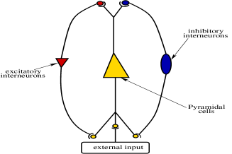
Figure 2: Schematic representation of the neural populations and their interactions, as considered in Jansen-Rit’s model [102].

This is therefore an activity-based model. The transfer functions $\alpha_{\cal E}$ and $\alpha_{\cal I}$ correspond respectively to excitatory and inhibitory post-synaptic potential (EPSP or IPSP). In the model introduced originally by Jansen and Rit, the synaptic integration is of first-order $\alpha(t)=Ke^{-\frac{t}{\tau}}H(t)$, where the coefficient $K,\tau$ are the same for the pyramidal and the excitatory population (denote them by $K_{\cal E},\tau_{\cal E}$), and different from the ones of the inhibitory population (denote them by $K_{\cal I},\tau_{\cal I}$). The sigmoid functions are the same whatever the populations. In Jansen-Rit’s approach the connectivity weights are assumed to be constant, equal to their mean value. Their equations, based on a naive mean-field approach, read therefore, with our notations [102, 82]:

$$\begin{cases}\frac{dA_{{\cal P}}}{dt}(t)&=-\,\frac{A_{{\cal P}}}{\tau_{\cal E}}+K_{\cal E}\,S(\bar{W}_{{\cal P}{\cal E}}\,A_{{\cal E}}(t)+\bar{W}_{{\cal P}{\cal I}}\,A_{{\cal I}}(t)+\alpha_{\cal E}\ast I(\cdot)+\alpha_{\cal E}\ast B(\cdot)),\\ \frac{dA_{{\cal E}}}{dt}(t)&=-\,\frac{A_{{\cal E}}}{\tau_{\cal E}}+K_{\cal E}\,S(\bar{W}_{{\cal E}{\cal P}}\,A_{{\cal P}}(t)),\\ \frac{dA_{{\cal I}}}{dt}(t)&=-\,\frac{A_{{\cal I}}}{\tau_{\cal I}}+K_{\cal I}\,S(\bar{W}_{{\cal I}{\cal P}}\,A_{{\cal P}}(t)).\end{cases}$$ (23)

A higher order model, where $\alpha(t)=K\frac{t}{\tau}e^{-\frac{t}{\tau}}H(t)$, was introduced by van Rotterdam and colleagues [174] to better account for the synaptic integration and to better reproduce the characteristics of real EPSP’s and IPSP’s. The bifurcation diagram of this version is quite richer than the Jansen-Rit one [82]. These equations are currently used in the neuroscience community either to provide activity models used for the analysis of signals obtained from imaging (MEG or Optical Imaging), or to provide dynamical models of epilepsy [53].

Role of synaptic weights variability

Let us now consider the more general case where synaptic weights have fluctuations about the mean value $\bar{W}_{ab}$. These variations dynamically differentiate the neurons within a population and may induce dramatic collective effects, when amplified by the nonlinear dynamics. Then, the actual evolution of a population can depart strongly from the first order mean-field approximation (not to speak of the naive mean-field approach).

Consider the local interaction field (20). Fix the trajectory of ${\bf V}=\left\{V_{i}\right\}_{i=1}^{N}$. Then, the $W_{ij}$’s being Gaussian, $\eta_{i}(t)$ is (conditionally) Gaussian, with mean:

$$\mathbb{E}\left[\eta_{i}(t)|{\bf V}\right]=\sum_{b=1}^{P}\bar{W}_{ab}\frac{1}{N_{b}}\sum_{j=1}^{N_{b}}S_{b}(V_{j}(t)),$$

where $\mathbb{E}\left[\right]$ is the expectation with respect to the $W_{ij}$’s distribution , and covariance:

$$Cov\left[\eta_{i}(t)\eta_{j}(s)|{\bf V}\right]=\delta_{ij}\sum_{b=1}^{P}\frac{\sigma^{2}_{ab}}{N_{b}}\sum_{j=1}^{N_{b}}S_{b}(V_{j}(t))S_{b}(V_{j}(s)),$$

where we have used that the $W_{ij}$’s are independent so that $Cov(W_{ij},W_{i^{\prime}j^{\prime}})=\delta_{ij}\delta_{i^{\prime}j^{\prime}}\frac{\sigma^{2}_{ab}}{N_{b}},\quad i\in a,j\in b$. Thus, conditionally to ${\bf V}$, and still assuming that there is a well defined thermodynamic limit, $\eta_{a}$ converges as $N\to\infty$ to a diagonal Gaussian process $\eta_{a}$ whose law depends only on the population, with mean:

$$\mathbb{E}\left[\eta_{a}(t)|{\bf V}\right]=\sum_{b=1}^{P}\bar{W}_{ab}\phi_{b}({\bf V}(t)),$$ (24)

and covariance:

$$Cov\left[\eta_{a}(t)\eta_{a}(s)|{\bf V}\right]=\sum_{b=1}^{P}\sigma^{2}_{ab}\lim_{N_{b}\to\infty}\frac{1}{N_{b}}\sum_{j=1}^{N_{b}}S_{b}(V_{j}(t))S_{b}(V_{j}(s))$$ (25)

Thus for a fixed trajectory, we find that the average value of $\eta_{a}$ obeys the same equation as in the first order mean-field approach, but it has now fluctuations and correlations given by (25).

The main difficulty is obviously that the trajectory ${\bf V}$ is generated by dynamics including the nonlinear and collective effects summarized in $\eta_{a}$. The following result can be shown [69]. As $N_{a}\to\infty$ the membrane potential of a neuron in population $V_{a}$ obeys the equation:

$$\sum_{l=0}^{k}a^{(l)}_{a}\frac{d^{l}V_{a}}{dt^{l}}(t)=\sum_{b=1}^{P}U_{ab}(t)+I_{a}(t)+B_{a}(t)$$ (26)

where $U_{ab}$, called the “mean-field interaction process”, is a Gaussian process, (thus entirely defined by its mean and covariance), statistically independent of the external noise $B$ and of the initial condition ${\bf V}(t_{0})$, and defined by:

$$\begin{cases}\mathbb{E}\left[U_{ab}(t)\right]=\bar{W}_{ab}m_{b}(t)\;\;\text{where \;\;}m_{b}(t)\stackrel{{\scriptstyle\rm def}}{{=}}\mathbb{E}[S_{b}(V_{b}(t))];\\ \mathrm{Cov}(U_{ab}(t),U_{ab}(s))=\sigma^{2}_{ab}\Delta_{ab}(t,s)\text{ where }\\ \qquad\qquad\Delta_{ab}(t,s)\stackrel{{\scriptstyle\rm def}}{{=}}\mathbb{E}\Big{[}S_{b}(V_{b}(t))S_{b}(V_{b}(s))\Big{]};\\ \mathrm{Cov}(U_{ab}(t),U_{cd}(s))=0\text{ if }a\neq c\text{ or }b\neq d.\end{cases}$$ (27)

One obtains therefore a set of self-consistent equations giving the mean and covariance of the mean-field interaction process $U_{ab}$. The interaction field of population $a$, $\eta_{a}$, is given by $\eta_{a}=\sum_{b=1}^{P}U_{ab}$, so that $\eta_{a}$ is indeed a Gaussian process with mean $\sum_{b=1}^{P}\bar{W}_{ab}m_{b}(t)$ in agreement with eq. (24), and covariance $\sum_{b=1}^{P}\sigma^{2}_{ab}\Delta_{ab}(t,s)$, in agreement with eq. (25). But there is a important distinction. Eq. (26), (27) provide the law of $U_{ab}$ and $\eta_{a}$, and provide a closed system of equations ruling the dynamical evolution of $V_{a}$ averaged over the distribution of $W_{ij}$’s, while in equations (24),(25) we only got the conditional law with respect to a fixed trajectory ${\bf V}$, henceforth leading to an incomplete formulation of the problem, since, to close the equations, one needs to know the probability distribution of the trajectories ${\bf V}$. This is an important distinction explaining the difference of notation between $\phi_{b}({\bf V}(t))$ in eq. (24) and $m_{b}(t)$ in (27).

Example: the simple model

Since $U_{ab}$ is a Gaussian process it is straightforward to obtain an explicit form for its mean and covariance as well as for the mean and covariance of $V_{a}$. In the case of the simple model (eq. (19)) this leads to the following equation for the evolution of the average value $\mu_{a}(t)$ of $V_{a}$:

$$\frac{d\mu_{a}}{dt}=-\frac{\mu_{a}}{\tau_{a}}+\sum_{\beta=1}^{P}\bar{W}_{ab}\int_{-\infty}^{+\infty}S_{b}\left(h\sqrt{v_{b}(t)}+\mu_{b}(t)\right)Dh+I_{a}(t),$$ (28)

with:

$$Dh=\frac{e^{-\frac{h^{2}}{2}}}{\sqrt{2\pi}}dh,$$ (29)

where $v_{a}(t)$ is the variance of $V_{a}$ at time $t$. Let $C_{ab}(t,s)$ be the covariance of $V_{a}(t),V_{b}(s)$. Then, $v_{a}(t)=C_{ab}(t,t)$. $C_{ab}(t,s)$ is given by [69]:

$$C_{ab}(t,s)=\delta_{ab}e^{-(t+s)/\tau_{a}}\Big{[}v_{a}(0)+\frac{\tau_{a}s_{a}^{2}}{2}\left(e^{\frac{2s}{\tau_{a}}}-1\right)+\sum_{b=1}^{P}\sigma^{2}_{ab}\int_{0}^{t}\int_{0}^{s}e^{(u+v)/\tau_{a}}\Delta_{b}(u,v)dudv\Big{]},$$ (30)

where:

$$\Delta_{b}(u,v)=\int_{{\sf I\!R}^{2}}S_{b}\left(x\frac{\sqrt{v_{b}(u)v_{b}(v)-C_{bb}(u,v)^{2}}}{\sqrt{v_{b}(v)}}+y\frac{C_{bb}(u,v)}{\sqrt{v_{b}(v)}}+\mu_{b}(u)\right)S_{b}\left(y\sqrt{v_{b}(v)}+\mu_{b}(v)\right)\,Dx\,Dy,$$ (31)

and where $s_{a}^{2}$ is the variance of a white noise $B_{i}(t)$ in (16) and where $Dx,Dy$ are Gaussian integrands of type (29).

These equations extend as well to more complex models, including the cortical columns model of Jansen-Rit [102] and van Rotterdam and colleagues [174] (see [69]). Therefore, the introduction of fluctuations in the synaptic distribution change drastically equations of evolution of such neural masses models as Jansen-Rit (see [69] for further comments).

2.1.3 Bifurcations of mean-field equations: a simple but non trivial example

Let us investigate these equations within details. In the case where fluctuations are neglected ($\sigma^{2}_{ab}=0,s_{\alpha}=0$), equations (30),(31) admit the trivial solution $C_{ab}(t,s)=0,v_{b}(t)=0$ and equation (28) reduces to the equation obtained by the naive mean-field approach. Incidentally, this validates the naive mean-field approach in this context. However, as soon as $\sigma^{2}_{ab}>0$ dynamics become highly non trivial since the mean-field evolution (28) depends on its fluctuations via the variance $v_{b}(t)$. This variance is in turn given by a complex equation requiring an integration on the whole past. Actually, unless one assumes the stationarity of the process, this equation cannot be written as an ordinary differential equation and the evolution is non-Markovian. This result, well known in the field of spin-glasses [18], has only been revealed recently in the field of neural masses models [69], though mean-field approaches were formerly used [163, 39, 36]. In these last papers, the role of mean-field fluctuations was clearly revealed and its influence on dynamics emphasized. In particular, chaotic dynamics have been exhibited, while the mean value $\mu_{a}(t)$ has a very regular and non chaotic behaviour (for example, it can be constant).

The model

As an example, let us consider the following model, corresponding to a time discretisation of (19) with $dt=\tau$ and only one population. Thus, synaptic weights are Gaussian with mean $\frac{\bar{W}}{N}$ and variance $\frac{\sigma^{2}}{N}$. Dynamics is given by:

$$V_{i}(t+1)=\sum_{j=1}^{N}W_{ij}S(V_{j}(t))+I_{i},\qquad i=1..N,$$ (32)

where $S$ is a sigmoidal function such as $S(x)=\tanh(gx)$ or $S(x)=\frac{1+\tanh(gx)}{2}$. The parameter $g$ controls the non-linearity of $S$. There is a time-constant current ${\bf I}$ whose components $I_{i}$ are random variables with mean $\bar{I}$ and variance $\sigma^{2}_{I}$.

The mean-field equations.

They write [39, 36]:

$$\mu(t+1)=\bar{W}\int_{\sf I\!R}S(h\sqrt{v(t)}+\mu(t))Dh+\bar{I},$$ (33)

$$v(t+1)=\sigma^{2}\int_{\sf I\!R}S^{2}(h\sqrt{v(t)}+\mu(t))Dh+\sigma^{2}_{I},$$ (34)

$$C(t+1,t^{\prime}+1)=\sigma^{2}\int_{{\sf I\!R}^{2}}S\left(\frac{\sqrt{v(t)v(t^{\prime})-C^{2}(t,t^{\prime})}}{\sqrt{v(t^{\prime})}}h+\frac{C(t,t^{\prime})}{\sqrt{v(t^{\prime})}}h^{\prime}+\mu(t)\right)S\left(h^{\prime}\sqrt{v(t^{\prime})}+\mu(t^{\prime})\right)DhDh^{\prime}+\sigma^{2}_{I},$$ (35)

where we have made $v(t)$ explicit, though it can be obtained from (35).

Let us comment these equations. First, they contain statistical parameters determining the probability distribution of synaptic weights and currents, $\bar{W},\sigma,\bar{I},\sigma_{I}$. They also contain an hidden parameter, $g$ determining the gain of the sigmoid, which is the same for all neurons. As we saw, deriving mean-field equations corresponds to substituting the analysis of the dynamical system (14), with a huge number of random microscopic parameters, by an “averaged” dynamical system depending on these few deterministic macroscopic parameters. In this spirit, we expect these equations to give indications about the generic behavior (in a probabilistic sense) when the synaptic weights and couplings are drawn according these values of macroscopic parameters, and when the number of neurons is large.

The variables $m,C$ essentially play the role of order parameters in statistical physics. They characterize the emergent behavior of a system with a large number of degree of freedom and they exhibit drastic changes corresponding, in statistical physics, to phase transitions, and in our context to a macroscopic bifurcations.

Bifurcations in mean-field equations.

Having these equations in hand, the idea is now to study the reduced dynamical system (33),(34),(35) and to infer information about the typical dynamics of (32). In the present example there exists a stationary regime of (33),(34),(35) and the stationary equations are given by:

$$\mu=\bar{W}\int_{\sf I\!R}S(h\sqrt{v}+\mu)Dh+\bar{I},\\$$ (36)

$$v=\sigma^{2}\int_{\sf I\!R}S^{2}(h\sqrt{v}+\mu)Dh+\sigma^{2}_{I},$$ (37)

$$C(t-t^{\prime})=\sigma^{2}\int_{{\sf I\!R}^{2}}S\left(\frac{\sqrt{v^{2}-C^{2}(t-t^{\prime})}}{\sqrt{v}}h+\frac{C(t-t^{\prime})}{\sqrt{v}}h^{\prime}+\mu\right)S\left(h^{\prime}\sqrt{v}+\mu\right)DhDh^{\prime}+\sigma^{2}_{I}.$$ (38)

These equations give important information about the statistical behavior of the model (32) with an increasing accuracy when the size increases. For example saddle-node bifurcations can be exhibited giving rise to bi-stability (see fig. 3 and [39] for more details). But, the most salient feature, as revealed by a detailed analysis of the complete set of equations (36), (37),(38), and especially of the equation for the time covariance (38)), is the existence of a chaotic regime, occurring for a sufficiently large non-linearity $g$. This chaotic region is delimited, in the space of parameters $\left(g,\bar{W},\sigma,\bar{I},\sigma_{I}\right)$, by a manifold whose equation is:

$$\sigma^{2}\int_{\sf I\!R}S^{\prime 2}(h\sqrt{v}+\mu)Dh=1.$$ (39)

Note that, in the case where $S(x)=\tanh(gx)$ this equation gives precisely the so-called De Almeida Thouless line [61], delimiting, in the Sherrington-Kirckpatrick model of spin-glasses [158], a frontier in the plane temperature-local external field, below which dynamics becomes highly non trivial. Here the parameter corresponding to the inverse temperature is $g$, while the external local field corresponds to ${\bf I}$. The “low temperature regime” of the SK model corresponds therefore to the chaotic regime of (32). This analogy is further discussed in [35, 36].

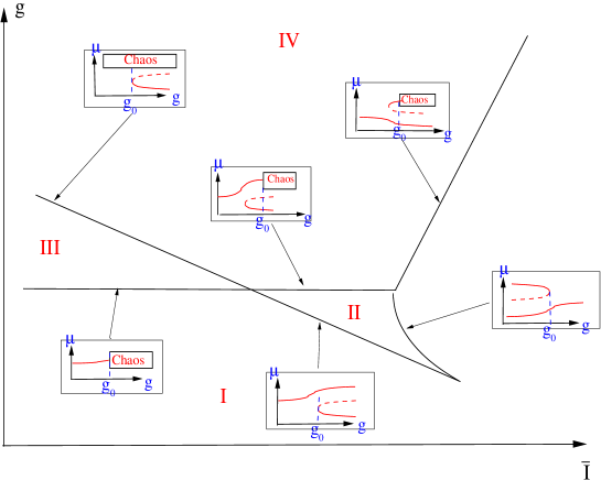
Figure 3: Schematic bifurcation map of model (32) in the plane $\bar{I},g$ (drawn from [39]). In the insets are represented the type of bifurcation occuring, for the mean-field equations, when crossing the line indicated by an arrow while increasing $g$ and keeping $\bar{I}$ constant. The bifurcation occurs for a value denoted $g_{0}$ in the inset. In these insets, the coordinates are $(g,\mu)$ where $\mu$ is given by eq. (36). The transition from a stable fixed point to chaos corresponds, for finite size systems to a Ruelle-Takens transition [153], while in infinite dimension ($N\to\infty$) this is a sharp transition (infinitely many eigenvalues of the Jacobian matrix at the fixed point crossing simultaneously the frontier of stability). Region I corresponds to a regime with one stable fixed point; region II to the coexistence of two stable fixed points; region III to a chaotic attractor and region IV to the coexistence of a stable fixed point and of a chaotic attractor.

Interpretation.

It can be shown that the crossing of this manifold corresponds, in the infinite system, to a sharp transition from fixed point to infinite dimensional chaos [35, 36]. Considering the finite size system, one can show that (32) exhibits generically a Ruelle Takens [153] transition to chaos as $g$ increases. As $N$ increases the transition to chaos occurs on a $g$ range becoming more and more narrow, giving this sharp transition in the thermodynamic limit. This is related to the fact that the eigenvalues of the Jacobian matrix accumulate on the stability circle as $N\to\infty$ [78] (see [36, 41] for details).

The interesting remark is that, considering only the naive mean-field equation (equation for the mean $\mu(t)$ with variance $v(t)=0$), one can easily exhibit examples (e.g. $S(x)=\tanh(gx)$ with no current) where $\mu(t)$ is a constant ($0$), while fluctuations are chaotic. This clearly shows the limits of the naive mean-field approach and the interest of analysing the role of fluctuations, not only in simple models such as (32) but also for more realistic models with several populations, like Jansen-Rit’s (23). Field fluctuations could reveal effects that do not appear in the naive mean-field approach and that could be measured in experiments. This question is under investigations (see the web page http://www-sop.inria.fr/odyssee/contracts/MACACC/macacc.html for more details).

2.2 Dynamics of conductance based Integrate and Fire Models

Let us now investigate a second type of collective dynamics, in the context of Integrate and Fire models introduced in section 1.2.1. These models have known a great success due to their (apparent) conceptual simplicity and analytical tractability [130, 68, 157, 169, 126, 79, 101] that can be used to explore some general principles of neurodynamics and coding. Surprisingly, the analysis of only one IF neuron submitted to a periodic current reveals already an astonishing complexity and the mathematical analysis requires elaborated methods from dynamical systems theory [110, 50, 51]. In the same way, the computation of the spike train probability distribution resulting from the action of a Brownian noise on an IF neuron is not a completely straightforward exercise [115, 77, 34, 33, 172] and may require rather elaborated mathematics. At the level of networks the situation is even more complex, and the techniques used for the analysis of a single neuron are not easily extensible to the network case. For example, Bressloff and Coombes [28] have extended the analysis in [110, 50, 51] to the dynamics of strongly coupled spiking neurons, but restricted to networks with specific architectures and under restrictive assumptions on the firing times. Chow and Kopell [49] studied IF neurons coupled with gap junctions but the analysis for large networks assumes constant synaptic weights. Brunel and Hakim [32] extended the Fokker-Planck analysis combined to a mean-field approach to the case of a network with inhibitory synaptic couplings but under the assumptions that all synaptic weights are equal. However, synaptic weights variability plays a crucial role in the dynamics, as we saw in the previous section (see also [176, 178, 175]). Note that the rigorous derivation of the mean-field equations, that requires large-deviations techniques [18], has not been yet done for the case of IF networks with continuous time dynamics (for the discrete time case see [165, 154]).

In this section, we present a rigorous result characterising the generic dynamics of a Generalised Integrate and Fire model, where time has been discretized according to the discussion of paragraph “raster plots” in section 1.2.1. We then give an example where we consider random synaptic weights.

2.2.1 Model

As we saw, the occurrence of a post-synaptic potential on synapse $j$, at time $t_{j}^{(n)}$, results in a change of membrane potential (eq. (8)). In conductance based models [149] this change is incorporated in the adaptation of conductances. The evolution of $V_{k}$, the membrane potential of neuron $k$, reads, setting the membrane capacity $C_{k}=1$ for simplicity:

$$\frac{dV_{k}}{dt}=-\frac{1}{\tau_{L}}\,(V_{k}-E_{L})-i_{k}^{(syn)}(V_{k},t,\left[\omega\right]_{0,t})+i_{k}^{(ext)}(t),$$ (40)

where $\left[\omega\right]_{0,t}$ is the raster plot up to time $t$. Recall that knowing $\left[\omega\right]_{0,t}$ is equivalent to knowing the list $\left\{t_{j}^{(n)}\right\}_{t}$ of firing times of all neurons up to time $t$. The first term in the r.h.s. is a leak term, $i_{k}^{(ext)}(t)$ is an external current, while:

$$i^{(syn)}_{k}(V_{k},t,\left[\omega\right]_{0,t})=(V_{k}-E^{+})\,\sum_{j\in{\cal E}}g_{kj}(t,\left[\omega\right]_{0,t})+(V_{k}-E^{-})\,\sum_{j\in{\cal I}}g_{kj}(t,\left[\omega\right]_{0,t}),$$

where $E^{\pm}$ are reversal potential (typically $E^{+}\simeq 0mV$ and $E^{-}\simeq-75mV$). As in the previous section, ${\cal E}$ and ${\cal I}$ refers respectively to excitatory and inhibitory neurons, and the $+$ ($-$) sign is relative to excitatory (inhibitory) synapses. Note that conductances are always positive thus the sign of the post-synaptic potential is determined by the reversal potentials $E^{\pm}$. At rest ($V_{k}\sim-70mV$) the $+$ term leads to a positive PSP while $-$ leads to a negative $PSP$.

Conductances depend on past spikes via the relation:

$$g_{kj}(t,\left[\omega\right]_{0,t})=G_{kj}\sum_{n=1}^{M_{j}(t,{\bf V})}\alpha_{j}(t-t_{j}^{(n)}).$$

In this equation, $M_{j}(t,{\bf V})=\sum_{s=0}^{t}\omega_{j}(s)$ is the number of times neuron $j$ has fired at time $t$. $G_{kj}$ is a positive constant proportional to the synaptic efficacy

$$\left\{\begin{array}[]{ccc}W_{kj}=E^{+}G_{kj}&\mbox{if}&\quad j\in{\cal E},\\ W_{kj}=E^{-}G_{kj}&\mbox{if}&\quad j\in{\cal I}.\end{array}\right.$$

Recall that we use the convention $W_{kj}=0$ if there is no synapse from $j$ to $k$

Then, we may write (40) in the form :

$$\frac{dV_{k}}{dt}+g_{k}V_{k}=i_{k},$$

(eq. (5) introduced in section 1.2.1) with:

$$g_{k}(t,\left[\omega\right]_{0,t})=\frac{1}{\tau_{L}}+\sum_{j=1}^{N}g_{kj}(t,\left[\omega\right]_{0,t}),$$

and:

$$i_{k}(t,\left[\omega\right]_{0,t})=\frac{E_{L}}{\tau_{L}}+E^{+}\,\sum_{j\in{\cal E}}g_{kj}(t,\left[\omega\right]_{0,t})+E^{-}\,\sum_{j\in{\cal I}}g_{kj}(t,\left[\omega\right]_{0,t})+i^{(ext)}_{k}(t).$$

This equation characterises the membrane potential evolution below the threshold $\theta$. Recall that, in Integrate and Fire models, if $V_{k}(t)\geq\theta$ then neuron membrane potential is reset instantaneously to some constant reset value $V_{reset}$ and a spike is emitted toward post-synaptic neurons.

2.2.2 Time discretisation

Using a time discretisation with a time step $\delta=1$, with the hypothesis discussed in section 1.2.1 leads to the following discrete-time model [45]:

$$V_{k}(t+1)=\gamma_{k}(t,\left[\omega\right]_{0,t})\left[1-Z(V_{k}(t))\right]V_{k}(t)+J_{k}(t,\left[\omega\right]_{0,t}),$$ (41)

where:

$$\gamma_{k}(t,\left[\omega\right]_{0,t})\stackrel{{\scriptstyle\rm def}}{{=}}e^{-\int_{t}^{t+1}\,g_{k}(s,\left[\omega\right]_{0,t})\,ds}<1,$$ (42)

is the integrated conductance over the time interval $[t,t+1[$,

$$J_{k}(t,\left[\omega\right]_{0,t})=\int_{t}^{t+1}i_{k}(s,\left[\omega\right]_{0,t})\,\nu_{k}(s,t+1,\left[\omega\right]_{0,t})\,ds,$$

is the corresponding integrated current with:

$$\nu_{k}(s,t+1,\left[\omega\right]_{0,t})=e^{-\int_{s}^{t+1}\,g_{k}(s^{\prime},\left[\omega\right]_{0,t})\,ds^{\prime}},$$

and where $Z$ is defined by :

$$Z(x)=\chi\left[x\geq\theta\right],$$ (43)

where $\chi$ is the indicator function that will later on allows us to include the firing condition in the evolution equation of the membrane potential (see (14)).

2.2.3 Generic dynamics

It can be shown that this systems has the following properties.

Singularity set.

The dynamics (14) (and the dynamics of continuous time IF models as well) is not smooth, but has singularities, due to the sharp threshold definition in neurons firing. The singularity set is:

$${\cal S}=\left\{{\bf V}\in{\cal M}|\exists i=1\dots N,\mbox{\ such \ that}\ V_{i}=\theta\right\}.$$

This is the set of membrane potential vectors such that at least one of the neurons has a membrane potential exactly equal to the threshold . This set has a simple structure: it is a finite union of $N-1$ dimensional hyperplanes. Although ${\cal S}$ is a “small” set both from the topological (non residual set) and probabilistic (zero Lebesgue measure) point of view, it has an important effect on the dynamics.

Local contraction.

The other important aspect is that the dynamics is locally contracting, because $\gamma_{k}(t,\left[\omega\right]_{0,t})<1$ (see eq. (42)). This has the following consequence. Let us consider the trajectory of a point ${\bf V}\in{\cal M}$ and perturbations with an amplitude $<\epsilon$ about ${\bf V}$ (this can be some fluctuation in the current, or some additional noise, but it can also be some error due to a numerical implementation). Equivalently, consider the evolution of the $\epsilon$-ball ${\cal B}({\bf V},\epsilon)$. If ${\cal B}({\bf V},\epsilon)\cap{\cal S}=\emptyset$ then the image of ${\cal B}({\bf V},\epsilon)$ is a ball with a smaller diameter. This means, that, under the condition ${\cal B}({\bf V},\epsilon)\cap{\cal S}=\emptyset$, a perturbation is damped. Now, if the images of the ball under the dynamics never intersect ${\cal S}$, any $\epsilon$-perturbation around ${\bf V}$ is exponentially damped and the perturbed trajectories about ${\bf V}$ become asymptotically indistinguishable from the trajectory of ${\bf V}$. This means that, if the membrane potential of neurons do not approach the threshold within a distance smaller than $\epsilon$ then perturbations of size smaller than $\epsilon$ are damped. Actually, there is a more dramatic effect. If all neurons have fired after a finite time $t$ then all perturbed trajectories collapse onto the trajectory of ${\bf V}$ after $t+1$ iterations. This loss of initial condition in a finite time is typical for IF models and is due to the reset of the membrane potential to a fixed value. For a discussion on IF model dynamics when this condition is relaxed see [113]. See also [79, 101].

Initial conditions sensitivity.

On the opposite, assume that there is a time, $t_{0}$, such that the image of the ball ${\cal B}({\bf V},\epsilon)$ intersects ${\cal S}$. By definition, this means that there exists a subset of neurons $\left\{i_{1},\dots,i_{k}\right\}$ and ${\bf V}^{\prime}\in{\cal B}({\bf V},\epsilon)$, such that $Z(V_{i}(t_{0}))\neq Z(V^{\prime}_{i}(t_{0}))$, $i\in\left\{i_{1},\dots,i_{k}\right\}$. For example, some neuron does not fire when not perturbed but the application of an $\epsilon$-perturbation induces it to fire (possibly with a membrane potential strictly above the threshold). This requires obviously this neuron to be close enough to the threshold. Clearly, the evolution of the unperturbed and perturbed trajectory may then become drastically different. Indeed, even if only one neuron is lead to fire when perturbed, it may induce other neurons to fire at the next time step, etc …, inducing an avalanche phenomenon leading to unpredictability and initial condition sensitivity.

It is tempting to call this behaviour “chaos”, but there is an important difference with the usual notion of chaos in differentiable systems. In the present case, due to the sharp condition defining the threshold, initial condition only occurs at sporadic instants, whenever some neuron is close enough to the threshold. Indeed, in certain periods of time the membrane potential typically is quite far below threshold, so that the neuron can fire only if it receives strong excitatory input over a short period of time. It shows then a behaviour that is robust against fluctuations. On the other hand, when membrane potential is close to the threshold a small perturbation may induce drastic change in the evolution.

Stability with respect to small perturbations.

Therefore, depending on parameters such as the synaptic efficacy, the external current, it may happen that, in the stationary regime, the typical trajectories stay away from the singularity set, say within a distance larger than $\epsilon>0$. Thus, a small perturbation (smaller than $\epsilon$) does not produce any change in the evolution. At a computational level, this robustness leads to stable input-output transformations.

On the other hand, if the distance between the set where the asymptotic dynamics lives and the singularity set is zero (or practically, very small) then the dynamics exhibit initial conditions sensitivity, and chaos. Typically a measure of this “distance” is given by [38]:

$$d(\Omega,{\cal S})=\inf_{{\bf V}\in\Omega}\inf_{t\geq 0}\min_{i=1\dots N}|V_{i}(t)-\theta|,$$ (44)

where $\Omega$ is the $\omega$-limit set.

Generic dynamics.

Now, the following theorem holds [45].

Theorem 1.

If $d(\Omega,{\cal S})>0$ then

1. $\Omega$ is composed of finitely many periodic orbits with a finite period,

2. There is a one-to-one correspondence between a trajectory on $\Omega$ and its raster plot,

3. There is a finite Markov partition.

Note however that $d(\Omega,{\cal S})>0$ is a sufficient but not a necessary condition to have a periodic dynamics. The main role of the condition $d(\Omega,{\cal S})>0$ is to avoid situations where the membrane potential of some neuron accumulates on $\theta$ from below (ghost orbits). This corresponds to a situation where the membrane potential of some “vicious” neuron fluctuates below the threshold, and approaches it arbitrary close, with no possible anticipation of its first firing time. This leads to an effective unpredictability in the network evolution, since when this neuron eventually fire, it may drastically change the dynamics of the other neurons, and therefore the observation of the past evolution does not allow one to anticipate what will be the future. In some sense, the system is in sort of a metastable state but it is not in a stationary state.

Now, assuming that conductances depend on past time only via a finite time horizon, one can show that,

Theorem 2.

Generically, in a probabilistic and topological sense, $d(\Omega,{\cal S})>0$.

(see [38] for the proof).

Discussion

Though the previous results suggests that dynamics is rather trivial since the first item tells us that dynamics is periodic, periods can however be quite long, depending on parameters. Indeed, following [38] an estimate for an upper bound on the orbits period is given by:

$$T\simeq 2^{N\frac{\log(d(\Omega,{\cal S}))}{\log(<\gamma>)}}$$ (45)

where $<\gamma>$ denotes the value of $\gamma$ averaged over time and initial conditions. Though this is only an upper bound this suggests that periods diverge when $d(\Omega,{\cal S})\to 0$. This is consistent with the fact that when $d(\Omega,{\cal S})$ is close to 0 dynamics “looks chaotic”. Therefore, $d(\Omega,{\cal S})$ is what a physicist could call an “order parameter”, quantifying somehow the dynamics complexity. The distance $d(\Omega,{\cal S})$ can be numerically estimated as done in [38, 45].

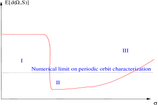
Figure 4: Sketch of the dynamical regimes exhibited by model (41) when synaptic weights are drawn at random with a Gaussian distribution ${\cal N}(0,\frac{\sigma^{2}}{N})$ (drawn from [38]). The expectation of $d(\Omega,{\cal S})$ under the $W_{ij}$’s distribution, $\mathbb{E}\left[d(\Omega,{\cal S})\right]$ , is drawn. It defines three regions. Region I corresponds to “neural death” (all neurons stop firing after a finite time); region II to a regime indistinguishable from chaos where the period of orbits are quite larger than what can be measured numerically; region III is a region where periodic orbits can be numerically detected.

Let us give an example of application of this result. Consider model (41) where the synaptic weights are drawn at random with a Gaussian distribution ${\cal N}(\frac{\bar{W}}{N},\frac{\sigma^{2}}{N})$, in the same spirit as in section 2.1. We have sketched the average value $d(\Omega,{\cal S})$, averaged over the distribution of the $W_{ij}$’s, as a function of $\sigma$, when $\bar{J}=0$ and $\gamma$ is fixed. The curve of $d(\Omega,{\cal S})$, as a function of $\sigma$, delimits 3 regions. Region I corresponds to “neural death” (all neurons stop firing after a finite time); region II to a regime indistinguishable from chaos where the period of orbits are quite larger than what can be measured numerically; region III is a region where periodic orbits can be numerically detected. This transition is reminiscent of the one exhibited in [110] for an isolated neuron submitted to a periodic excitation, but the present analysis hold at the network level.

Let us now discuss the second item of theorem 1. It expresses that the raster plot is a symbolic coding for the membrane potential trajectory. In other words there is no loss of information about the dynamics when switching from the membrane potential description to the raster plot description. This is not true anymore if $d(\Omega,{\cal S})=0$. This issue, as well as the existence of a Markov partition, is used in section 3.

2.3 Conclusion

In this section we have shown two examples of classical neural networks models, where the use of combined techniques from dynamical systems theory, statistical physics and probability theory allows the characterization of the dynamical regimes generically occurring. Moreover, considering random and independent synaptic weights $W_{ij}$’s we have been able to obtain a phenomenological “bifurcation diagram” where one replaces the overwhelming number of control parameters ($N^{2}$ synaptic weights plus additional parameters defining the external current) by a small set of statistical parameters controlling the probability distribution of the $W_{ij}$’s (mean and variance). This diagram characterizes the average behaviour of many different copies of the neural network when the $W_{ij}$’s are drawn at random with a specific value of their mean and variance. It does not tell us what will be the typical behaviour of a given network (i.e. a given realization of the $W_{ij}$’s). Moreover, for the mean-field approach reported in section 2.1 the bifurcation map corresponds to taking the limit $N\to\infty$ where, e.g. the transition to chaos is easy to represent since it is sharp. The situation is radically different for finite $N$ where the “edge of chaos” associated with the transition by quasi-periodicity is rather complex and results from the overlapping of Arnold tongues [121, 73]. For the gIF model, theorem 1 and 2 hold for generic values of the synaptic weights $W_{ij}$’s hence they apply to the huge space of parameters $\boldsymbol{\gamma}$. Moreover, they characterize generic behaviours both in a topological and probabilistic sense. However, to figure out how $d(\Omega,{\cal S})$ looks like we focused actually on the same situation as in section 2.1 where the $W_{ij}$’s are drawn at random, independently, where we study the effect of their variance of the average value of $d(\Omega,{\cal S})$. It seems possible to have an analytic expression of $d(\Omega,{\cal S})$, but this requires to take the “thermodynamic limit” $N\to\infty$ (Cessac and Touboul, in preparation).

Thus, it appears clearly that these approaches are limited

1. By the assumption of independence of the $W_{ij}$’s.

2. By the necessity of taking the limit $N\to\infty$ to obtain analytic expression.

These limitations are further discussed in the conclusion section 6.

3 Spikes trains statistics

As we have seen in section 1, neuronal activity is manifested by emission of spike trains having a wide variety of forms (isolated spikes, periodic spiking, bursting, tonic spiking, tonic bursting, etc) [99, 30, 171], depending on physiological parameters, but also on excitation coming either from other neurons or from external sources. From these evidences, it seems natural to consider spikes as “information quanta” or “bits” and to seek the information exchanged by neurons in the structure of spike trains. Doing this, one switches from the description of neurons in terms of membrane potential dynamics, to a description in terms of spikes trains and raster plots. Though this change of description raises many questions it is commonly admitted in the computational neuroscience community that spike trains contain the “neural code”.

Admitting this raises however other questions. How is “information” encoded in a spike train: rate coding [5], temporal coding [167], rank coding [140, 62], correlation coding [105] ? How to measure the information content of a spike train ? There is a wide literature dealing with these questions [136, 104, 14, 135, 9, 160, 74, 138], which are inherently related to the notion of statistical characterisations of spike trains, see [145, 60, 76] and references therein for a a review. As a matter of fact, a prior to handle “information” in a spike train is the definition of a suitable probability distribution that matches the empirical averages obtained from measures.

3.1 Spike responses of neurons

Neurons respond to excitations or stimuli by finite sequences of spikes. Thus, the dynamical response $R$ of a neuronal network to a stimuli $S$ (which can be applied to several neurons in the network), is a sequence $\boldsymbol{\omega}(t)\dots\boldsymbol{\omega}(t+\tau)$ of spiking patterns. “Reading the neural code” means that one seeks a correspondence between responses and stimuli. However, the spike response does not only depend on the stimulus, but also on the network dynamics and therefore fluctuates randomly. Thus, the spike response is sought as a conditional probability $P(R|S)$ [145] and “reading the code” consists of inferring $P(S|R)$ e.g. via Bayesian approaches, providing a loose dictionary where the observation of a fixed spikes sequences $R$ does not provide a unique possible stimulus, but a set of stimuli, with different probabilities. Having models for conditional probabilities $P(R|S)$ is therefore of central importance. For this, one needs a good notion of statistics.

These statistics can be obtained in two different ways. Either one repeats a large number of experiments, submitting the system to the same stimulus $S$, and performs a sample averaging. This approach relies on the assumption that the system has the same statistical properties during the whole set of experiments (i.e. the system has not evolved, adapted or undergone bifurcations meanwhile). Or, one performs a time average. For example, to compute $P(R|S)$, one counts the number of times $n(R,T,\omega)$ when the finite sequence of spiking patterns $R$, appears in a spike train $\omega$ of length $T$, when the network is submitted to a stimulus $S$. Then, the probability $P(R|S)$ is estimated by:

$$P(R|S)=\lim_{T\to\infty}\frac{n(R,T,\omega)}{T}.$$

This approach implicitly assumes that the system is in a stationary state.

The empirical approach is often “in-between”. One fixes a time window of length $T$ to compute the time average and then performs an average over a finite number ${\cal N}$ of experiments corresponding to selecting different initial conditions. In any case the implicit assumptions are essentially impossible to control in real (biological) experiments, and difficult to prove in models. So, they are basically used as “working” assumptions. To summarise, one observes, from ${\cal N}$ repetitions of the same experiment, ${\cal N}$ raster plots $\omega_{m},m=1\dots\cal N$ on a finite time horizon of length $T$. From this, one computes experimental averages allowing to estimate $P(R|S)$ or, more generally, to estimate the average value, $\langle\phi\rangle$, of some prescribed observable $\phi(\omega)$. These averages are estimated by :

$$\bar{\phi}^{({\cal N},T)}=\frac{1}{{\cal N}T}\sum_{m=1}^{{\cal N}}\sum_{t=1}^{T}\phi({\sigma^{t}_{\boldsymbol{\gamma}}}\omega_{m}).$$ (46)

Typical examples of such observables are $\phi(\omega)=\omega_{i}(0)$ in which case $\langle\phi\rangle$ is the firing rate of neuron $i$; $\phi(\omega)=\omega_{i}(0)\omega_{j}(0)$ then $\langle\phi\rangle$ measures the probability of spike coincidence for neuron $j$ and $i$; $\phi(\omega)=\omega_{i}(\tau)\omega_{j}(0)$ then $\langle\phi\rangle$ measures the probability of the event “neuron $j$ fires and neuron $i$ fires $\tau$ time step later” (or sooner according to the sign of $\tau$). In the same way $P(R|S)$ is the average of the indicatrix function $\chi_{R}(\omega)=1$ if $\omega\in R$ and $0$ otherwise, the statistics being performed when the neuronal network is submitted to $S$. Note that in (46) we have used the shift ${\sigma^{t}_{\boldsymbol{\gamma}}}$ for the time evolution of the raster plot. This notation is more compact and more adapted to the next developments than the classical formula, reading, e.g., for firing rates $\frac{1}{{\cal N}T}\sum_{m=1}^{{\cal N}}\sum_{t=1}^{T}\phi(\boldsymbol{\omega}_{m}(t))$.

This estimation depends on $T$ and ${\cal N}$. However, one expects that, as ${\cal N},T\to\infty$, the empirical average $\bar{\phi}^{({\cal N},T)}$ converges to the theoretical average $\langle\phi\rangle$, as stated e.g. from the law of large numbers. Unfortunately, one usually does not have access to these limits, and one is lead to extrapolate theoretical averages from empirical estimations. The main difficulty is that these observed raster plots are produced by an underlying dynamics which is usually not explicitly known (as it is the case in experiments) or impossible to fully characterise (as it is the case in most large dimensional neural networks models). Thus, one is constrained to propose ad hoc statistical models. As a matter of fact, the choice of a statistical model always relies on assumptions. Here we make an attempt to formulate these assumptions in a compact way with the widest range of application. These assumptions are compatible with the statistical models commonly used in the literature like Poisson models or Ising like models à la Schneidman and collaborators [155], but lead also us to propose more general forms of statistics. Moreover, our approach incorporates additional elements such as the consideration of neurons dynamics, and the fact that this dynamics severely constrain the set of admissible raster plots, $\Sigma_{\boldsymbol{\gamma}}$. This last issue is, according to us, fundamental, and, to the best of our knowledge, has never been considered before in this field.

On this basis we propose the following definition. Fix a set $\phi_{l}$, $l=1\dots K$, of observables, i.e. functions $\Sigma_{\boldsymbol{\gamma}}\to{\sf I\!R}$ which associate real numbers to sequences of spiking patterns. Assume that the empirical average (46) of these functions has been computed, for a finite $T$ and ${\cal N}$, and that $\bar{\phi_{l}}^{(T,{\cal N})}=C_{l}$.

A statistical model is a probability distribution $\nu$ on the set of raster plots such that:

1. $\nu(\Sigma_{\boldsymbol{\gamma}})=1$, i.e. the set of non admissible raster plots has a zero $\nu$-probability.

2. $\nu$ is ergodic for the left-shift ${\sigma_{\boldsymbol{\gamma}}}$.

3. For all $l=1\dots K$, $\nu(\phi_{l})=C_{l}$, i.e., $\nu$ is compatible with the empirical averages.

Note that item 2 amounts to assuming that statistics are invariant under time translation. On practical grounds, this hypothesis can be relaxed using sliding time windows. This issue is discussed in more details in [40]. Note also that $\nu$ depends on the parameters $\boldsymbol{\gamma}$. Assuming that $\nu$ is ergodic has the advantage that one does not have to average both over experiments and time. It is sufficient to focus on time average for a single raster plot, via the time-empirical average:

$$\pi_{\omega}^{(T)}(\phi)=\frac{1}{T}\sum_{t=1}^{T}\phi({\sigma^{t}_{\boldsymbol{\gamma}}}\omega).$$ (47)

3.2 Raster plots statistics.

A canonical way to construct statistical models comes from statistical physics [103]. This approach has been introduced for spike train analysis by [155] and generalised in [40]. According to item (1)-(3) we are seeking a probability distribution $\nu$ which matches the constraints $\nu(\phi_{l})=C_{l},\ l=1\dots K$, where $\nu(\phi_{l})$ is the average of $\phi_{l}$ under $\nu$. We want to stick on these constraints, imposed by experimental results, without adding any other hypothesis. In the realm of statistical physics this amounts to maximising the statistical entropy under the constraints $\nu(\phi_{l})=C_{l},\ l=1\dots K$. In the context of the so-called thermodynamic formalism of ergodic theory, which is a quite powerful tool to handle such statistical problems, this amounts to solving the following variational principle:

$$P\left[\boldsymbol{\psi}\right]=\sup_{\nu\in m^{(inv)}}(h\left[\nu\right]+\nu\left[\boldsymbol{\psi}\right]),$$ (48)

where $m^{(inv)}$ is the set of invariant (stationary) measures for the dynamics and $h$ is the entropy rate. We have introduced a “potential”,

$$\boldsymbol{\psi}=\sum_{l=1}^{K}\lambda_{l}\phi_{l},$$ (49)

where the $\lambda_{l}$’s are adjustable Lagrange multipliers. A probability measure ${\nu_{\scriptstyle{\boldsymbol{\psi}}}}$ which realises the supremum, i.e.

$$P\left[\boldsymbol{\psi}\right]=h\left[{\nu_{\scriptstyle{\boldsymbol{\psi}}}}\right]+{\nu_{\scriptstyle{\boldsymbol{\psi}}}}\left[\boldsymbol{\psi}\right],$$

is called an “equilibrium state”. The function $P\left[\boldsymbol{\psi}\right]$ is called the “topological pressure” in the realm of ergodic theory, and “thermodynamic potential” (free energy, free enthalpy, pressure) in statistical physics. Note that ergodic theory imposes less constraints on dynamics than statistical physics (the microscopic dynamics does not need to be Hamiltonian). From the topological pressure one computes the moments of the distribution ${\nu_{\scriptstyle{\boldsymbol{\psi}}}}$. In particular,

$$\frac{\partial P\left[\boldsymbol{\psi}\right]}{\partial\lambda_{l}}={\nu_{\scriptstyle{\boldsymbol{\psi}}}}(\phi_{l}).$$ (50)

This relation fixes the value of the Lagrange multipliers $\lambda_{l}$ in order to have ${\nu_{\scriptstyle{\boldsymbol{\psi}}}}(\phi_{l})=C_{l}$.

Moreover, in “good cases” (e.g. uniformly hyperbolic dynamical systems), equilibrium states are also Gibbs states [25, 26, 112, 139, 47]. A Gibbs state, or Gibbs measure, is a probability measure such that, one can find some constants $c_{1},c_{2}$ with $0<c_{1}\leq 1\leq c_{2}$ such that for all $n\geq 1$ and for all $\omega$:

$$c_{1}\leq\frac{{\nu_{\scriptstyle{\boldsymbol{\psi}}}}\left(\omega\in\left[\omega\right]_{0,n-1}\right)}{\exp(-nP\left[\boldsymbol{\psi}\right]+S^{(n)}\boldsymbol{\psi}(\omega))}\leq c_{2},$$ (51)

where $S^{(n)}\boldsymbol{\psi}(\omega)=\sum_{t=0}^{n-1}\boldsymbol{\psi}({\sigma^{t}_{\boldsymbol{\gamma}}}\omega)$ and where we denote by $\left[\omega\right]_{0,n-1}$ a cylinder set of length $n$, namely the set of raster plots $\omega^{\prime}$ such that $\boldsymbol{\omega}^{\prime}(t)=\boldsymbol{\omega}(t),t=0\dots n-1$. Basically, this means that the probability that a raster plot starts with the bloc $\left[\omega\right]_{0,n-1}$ behaves like $\frac{\exp(S^{(n)}\boldsymbol{\psi}(\omega))}{Z_{n}}$. One recognises the classical Gibbs form where space translation in lattice system is replaced by time translation (shift ${\sigma^{t}_{\boldsymbol{\gamma}}}$) and where the normalisation factor $Z_{n}$ is the partition function. Note that $P\left[\boldsymbol{\psi}\right]=\limsup_{n\to\infty}\frac{1}{n}\log Z_{n}$, so that $P\left[\boldsymbol{\psi}\right]$ is indeed the formal analog of a thermodynamic potential (like free energy).

In this context, the probability of a spiking pattern block $R=\left[\boldsymbol{\omega}\right]_{0,n-1}$ of length $n$ corresponding to the response $R$ to a stimuli $S$ “behaves like” (in the sense of eq. (51)):

$$P\left[R|S\right]=\nu\left[\omega\in R|S\right]\sim\frac{1}{Z_{n}\left[\lambda_{1}(S),\dots,\lambda_{l}(S)\right]}\exp\left[\sum_{l=1}^{K}\lambda_{l}(S)\sum_{t=0}^{n-1}\phi_{l}({\sigma^{t}_{\boldsymbol{\gamma}}}\omega)\right],$$ (52)

where the $\lambda_{l}$’s depend on the stimulus $S$. Obviously, for two different stimuli the probability $P(R|S)$ may drastically change.

3.3 Examples.

Firing rates. If $\phi_{l}(\omega)=\omega_{l}(0)$, then ${\pi_{\omega}^{(T)}}(\phi_{l})=r_{l}$ is the average firing rate of neuron $l$ within the time period $T$. Then, the corresponding statistical model is a Bernoulli distribution where neuron $l$ has a probability $r_{l}$ to fire at a given time. The probability that neuron $l$ fires $k$ times within a time delay $n$ is a binomial distribution and the inter-spike interval is Poisson distributed [77].

Spikes coincidence. If $\phi_{l}(\omega)\equiv\phi_{(i,j)}(\omega)=\omega_{i}(0)\,\omega_{j}(0)$ where, here, the index $l$ is an enumeration for all (non-ordered) pairs $(i,j)$, then the corresponding statistical models has the form of an Ising model, as discussed by Schneidman and collaborators in [155, 170]. As shown by these authors in experiments on the salamander retina, the probability of spike blocs estimated from the “Ising” statistical model fits quite better to empirical date than the classical Poisson model.

Enlarged spikes coincidence. As a generalisation one may consider the probability of co-occurrence of spikes from neuron $i$ and $j$ within some time interval $\tau$. The corresponding functions are $\phi_{l}(\omega)=\omega_{i}(0)\omega_{j}(\tau)$ and the probability of a spike bloc $R$ reads:

$$P\left[R|S\right]=\frac{1}{Z_{n}\left[\lambda_{1,1}(S),\dots,\lambda_{N,N}(S)\right]}\exp\left[\sum_{i\leq j}\lambda_{ij}(S)\sum_{t=0}^{n-1}\omega_{i}(t)\,\omega_{j}(t+\tau)\right].$$

An example is provided in section 5.3.

Further generalisations can be considered as well.

Generalised Integrate and Fire models Due to their particular structure and especially the fact that generically a Markov partition exists, gIF models of type (41) are explicit examples where this theory gives striking results (see [40] for details and section 5 for an application to the effect of synaptic plasticity to spike trains statistics.)

3.4 Validating a statistical model

There are currently huge debates on the way how brain encodes information. Are frequency rates sufficient to characterise the neural code [175] ? Are pair correlations significant ? Do higher order statistics matter ? Actually, it might be that the answer depend on the brain process under consideration and some peoples actually believe that “brain speaks several languages and speak all of them at the same time” (Franck Grammont, private communication. For a nice illustration of this see [80]). These questions are inherently linked to the notion of (i) finding statistical models; (ii) discriminate several statistical models and select the “best one”.

Let us consider an illustrative example, i.e. the question: are correlations significant ? Answering this question is a crucial issue for biologists/experimentalists [156, 141, 142]. Note that it has absolutely no meaning to try and answer this question from empirical data when considering “the brain” as a whole. But, as emphasised by [148], there is maybe some hope to make one step forward when considering small neural assemblies (e.g. small pieces of retina).

Moreover this question has no “absolute” answer but a relative answer in the following sense. Let us consider the 1st order potential:

$$\boldsymbol{\psi}_{1}(\omega)=\sum_{i=1}^{N}\lambda_{i}\,\omega_{i}(0),$$

thus only taking firing-rates into account, “against” the 2nd order potential:

$$\boldsymbol{\psi}_{2}(\omega)=\sum_{i=1}^{N}\lambda_{i}\,\omega_{i}(0)+\sum_{i,j=1}^{N}\sum_{\tau=-T_{s}}^{T_{s}}\lambda_{ij\tau}\,\omega_{i}(0)\omega_{j}(\tau),$$

where $T_{s}$ is a characteristic time scale. This potential form takes both firing-rate and correlations into account.

The realm of thermodynamic formalism offers a numerically tractable way to compare the statistical models related to these two potentials. The relative entropy or Kullback-Leibler divergence between a Gibbs measure ${\nu_{\scriptstyle{\boldsymbol{\psi}}}}$ and a stationary measure $\mu$ is given by [112, 46, 47]:

$$h\left(\mu|{\nu_{\scriptstyle{\boldsymbol{\psi}}}}\right)=P\left[\boldsymbol{\psi}\right]-\int\boldsymbol{\psi}d\mu-h(\mu).$$

In the present case, we are given an empirical measure, ${\pi_{\omega}^{(T)}}$, (see eq. (47)), obtained from experiments. To discriminate between the two potentials $\boldsymbol{\psi}_{1},\boldsymbol{\psi}_{2}$ a possible criterion consists of choosing the potential which minimises the relative entropy of the corresponding Gibbs measure with respect to the empirical measure. Namely, if there is $T_{0}>0$ such that, for all $T\geq T_{0}$ :

$$h({\pi_{\omega}^{(T)}}\,|\,\nu_{\boldsymbol{\psi}_{1}})<h({\pi_{\omega}^{(T)}}\,|\,\nu_{\boldsymbol{\psi}_{2}})$$ (54)

then $\boldsymbol{\psi}_{1}$ is considered as a better statistical model than $\boldsymbol{\psi}_{2}$. The nice thing is that, using the thermodynamic formalism, one can develop algorithms allowing such a comparison (Cessac, Vasquez, Viéville, in preparation).

3.5 Conclusion

When analysing spike train statistics, one is lead to propose several statistical models corresponding to distinct hypothesis. For example, characterising inter-spike interval distribution by a homogeneous Poisson process ultimately corresponds to assuming that correlations between neurons and time correlations are irrelevant and that frequency rates are sufficient to characterise statistics. In our presentation this amounts to considering a Gibbs potential of form $\sum_{i=1}^{N}\lambda_{i}\omega_{i}(0)$. More general forms can be proposed as well. But this leads to two fundamental questions:

1. How to discriminate statistical models from empirical data ? This is a crucial issue, whose tractability was deeply raised by and Roudy and his collaborators in a very recent paper [148]. Many criteria used in the literature rely on the computation of the Kullback-Leibler divergence. We have shown how the use of the thermodynamic formalism, relying on a safe recipe from statistical mechanics, could allow to compute this quantity from data.

2. Instead of defining the statistical model from ad hoc observables, is it possible to propose a canonical form relying on some generic principle ? This issue is addressed in section 5.3 where we consider the effect of synaptic plasticity on spike trains statistics.

4 Interplay between synaptic graph structure and neurons dynamics.

4.1 Causal actions

Since synapses are used to transmit neural fluxes (spikes) from a neuron to another one, the existence of synapses between a neuron (A) and another one (B) is implicitly attached to a notion of “influence” or causal and directed action. However, as we saw, a neural network is a highly dynamical object and its behavior is the result of a complex interplay between the neurons dynamics and the synaptic network structure. Moreover, the neuron $B$ receives usually synapses from many other neurons, each them being “influenced” by many other neurons, possibly acting on $A$, etc… Thus the actual “influence” or action of A on B has to be considered dynamically and in a global sense, by considering $A$ and $B$ not as isolated objects, but, instead, as entities embedded in a system with a complex interwoven dynamical evolution. In this context it is easy to imagine examples where there is a synapse from $A$ to $B$ but no clear cut influence, or, in the opposite, no synapse and nevertheless an effective action.

Thus, one has to consider topological aspects (such as the feedback circuits) and dynamical aspects. One way of doing this is to compute correlations between neurons (cross-correllogramms). However, correlations functions do not provide causal information. A strong correlation between $A$ and $B$ at time $t$ does not tell us if $A$ acts on $B$ or if $B$ acts on $A$ (note in particular that $C_{AB}(t)=C_{BA}(-t)$).

Another way consists of exciting neuron $A$, say with a weak signal, and observe the effects on $B$, e.g. by comparing its evolution with and without the signal applied on $A$. A natural choice for an excitatory signal is a periodic signal, with a tunable frequency. Thus, the response function, drawn versus frequency, provides similar information as the complex susceptibility in Physics. In particular, peaks in the susceptibility corresponds to resonances, that is, a response of maximal amplitude. These resonances can be used to provide an effective, frequency dependent notion of network structure, as we now show.

4.2 A simple but non trivial example

Consider the model (32) where neurons are represented by frequency rates. As we saw in section 2.1.3 this model exhibit, in finite dimension $N$ a generic transition to chaos by quasi-periodicity, when increasing the non-linearity of the sigmoidal transfer function $S$.

Signal propagation and effects of non-linearity.

Assume that this system is in the chaotic regime. Note that the corresponding Fourier spectrum is not flat but contains peaks (resonances) reminiscent of the transition by quasi-periodicity [43]. Assume now that we superimpose upon the membrane potential $V_{j}(t)$ of the neuron $j$ a small external signal $\xi_{j}(t)$. Does this signal have an effect which propagates inside the network ? and how ? Because of the sigmoidal shape of the transfer functions the answer depends crucially, not only on the connectivity of the network, but also on the value of the $V_{k}$’s. Assume, for the moment and for simplicity, that the time-dependent signal $\xi_{j}(t)$ has variations substantially faster than the variations of $V_{j}$. Consider then the cases depicted in Fig. 5. In the first case (a) the signal $\xi_{j}(t)$ is amplified by $S$, without distortion if $\xi_{j}(t)$ is weak enough. In the second case (Fig. 5b), it is damped and distorted by the saturation of the sigmoid. More generally, when considering the propagation of this signal from the node $j$ to some node $i$ one has to take into account the level of saturation of the nodes encountered in the path, but the analysis is complicated by the fact that the nodes have their own dynamical evolution (Fig. 5c).

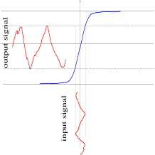
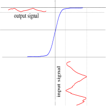
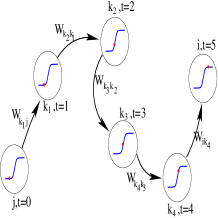
Figure 5: Nonlinear effects induced by a transfer function with a sigmoidal shape on signal transmission. Fig. 5a (left). Amplification. Fig. 5b (middle). Saturation. Fig. 5c (right). The propagation of a signal along a path in the network depends not only on the weights of the links but also on the level of saturation of the nodes that the signal meets. The level of saturation depends on the current state of the node (schematically represented as a red point in the figure). This state evolves with time.

Tangent space splitting.

In this context we would like to measure the average “influence” of neuron $A$ on neuron $B$ (namely how a weak signal applied on $A$ perturbs on average the state of $B$), including the effects of the nonlinear dynamics. Typically, in dissipative systems, such as neural networks models, where volume in the phase space is dynamically contracted, dynamics asymptotically settle “onto” attractors. Examples of attractors are stable fixed points, or stable periodic orbits. Chaotic attractors have moreover the following property. While dynamics transverse to the attractor is contracting (corresponding precisely to the attractivity property), dynamics “parallel” to the attractor is expanding, corresponding to initial condition sensitivity. In other words, the tangent space of attractor points can be split into a contracting and an expanding part (see fig. 6).

Structural properties of chaotic attractors are usually characterized by statistical quantities such as Lyapunov exponents. There is indeed a natural notion of average in chaotic systems related to the Sinai-Ruelle-Bowen measure $\rho$ (SRB) [159, 25, 150] which is obtained as the (weak) limit of the Lebesgue measure $\mu$ under the dynamical evolution:

$$\rho=\lim_{n\to+\infty}{\bf F}_{\boldsymbol{\gamma}}^{n}\mu.$$

where ${\bf F}_{\boldsymbol{\gamma}}^{n}$ is the $n$-th iterate of ${\bf F}_{\boldsymbol{\gamma}}$. Following an orbit upon the attractor it is possible to characterize the average expansion and contraction rates for this orbit via Lyapunov exponents. A positive Lyapunov exponent indicates local expansion while a negative one indicates contraction.

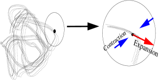
Figure 6: Sketch of an attractor and of the decomposition of the tangent space into contracting and expanding directions. A perturbation in the contracting space leads to a trajectory which converges back to the attractor. A perturbation in the transverse direction leads to a trajectory staying onto the attractor but which separates from the mother trajectory. This representation is made for a discrete time system. Note that the regular spacing between points is an artefact of the representation.

In the following we will assume that all Lyapunov exponents are bounded away from zero. Then for each ${\bf V}\in supp\,\rho$, where $supp\,\rho$ is the support of $\rho$, there exists a splitting $E^{(s)}_{{\bf V}}\oplus E^{(u)}_{\bf V}$ such that $E^{(u)}_{\bf V}$, the unstable space, is locally tangent to the attractor (the local unstable manifold) and $E^{(s)}_{\bf V}$, the stable space, is transverse to the attractor (locally tangent to the local stable manifold). Let us emphasize that the stable and unstable spaces depend on ${\bf V}$ (while the Lyapunov exponents are $\mu$ almost surely constant).

Let us consider a point ${\bf V}$ upon the attractor and make a small perturbation $\delta_{\bf V}$. This perturbation can be decomposed as $\delta_{\bf V}=\delta_{\bf V}^{(u)}+\delta_{\bf V}^{(s)}$ where $\delta_{\bf V}^{(u)}\in E^{(u)}_{{\bf V}}$ and $\delta_{\bf V}^{(s)}\in E^{(s)}_{\bf V}$. $\delta_{\bf V}^{(u)}$ is locally amplified with an exponential rate (given by the largest positive Lyapunov exponent). On the other hand $\delta_{\bf V}^{(s)}$ is damped with an exponential speed (given by the smallest negative Lyapunov exponent)

Linear response.

Assume now that we superimpose a signal of weak amplitude, considered as an external current, upon some neuron ($k$) in such a way that the dynamics is still chaotic (with only a tiny variation of the Lyapunov exponents). For simplicity, we suppose that the signal does not depend on the state of the system, but we can consider this generalization without difficulty (linear response still applies in this case, but equations (55), (56) do not hold anymore). Denote by $\bm{\xi}$ the vector $\left\{\xi_{i}\right\}_{i=1}^{N}$. The new dynamical system is described by the equation:

$$\widetilde{V}(t+1)={{\bf F}_{\boldsymbol{\gamma}}}\left[\widetilde{V}(t)\right]+\bm{\xi}(t).$$

The weak signal $\bm{\xi}(t)$ may be viewed as a small perturbation of the trajectories of the unperturbed system (32). At each time this perturbation has a decomposition $\bm{\xi}(t)=\bm{\xi}^{(s)}(t)+\bm{\xi}^{(u)}(t)$ on the local stable and unstable spaces. The stable component $\bm{\xi}^{(s)}(t)$ is exponentially damped. The unstable one $\bm{\xi}^{(u)}(t)$ is amplified by the dynamics and then scrambled by the nonlinear terms. Consequently, it is impossible to predict the long term effect of signal $\bm{\xi}(t)$ on the global dynamics.

This is true for individual trajectories. However, the situation is substantially different if one considers the average effect of the signal, the average being performed with respect to the SRB measure $\rho$ of the unperturbed system. Indeed, as an application of the general theory [151], it has been established in [42, 43, 44] that the average variation $\delta_{V_{i}}(t)$ of the membrane potential $V_{i}$ under the influence of the signal is given, to the linear order, by:

$$\left<\widetilde{V}_{i}(t)-V_{i}(t)\right>=\sum_{\sigma=0}^{\infty}\sum_{j}\chi_{ij}(\sigma)\xi_{j}(t-\sigma-1).$$ (55)

We used the shortened notation $<\ >$ for the average with respect to $\rho$. In this expression $\chi_{ij}(\sigma)$ are the matrix elements of :

$$\chi(\sigma)=\int\rho(d{\bf V})D{\bf F}^{\sigma}_{{\bf V}}.$$ (56)

Thus $\chi(\sigma)$ is a matrix representing the average value of the iterate $\sigma$ of the Jacobian matrix. Let us note that the fact that $\chi(\sigma)$ remains bounded for $\sigma\to\infty$ is not a trivial result because $D{\bf F}^{\sigma}_{{\bf V}}$ diverges exponentially with $\sigma$. The convergence of $\chi(\sigma)$ has been rigorously shown by Ruelle under the hypothesis of uniform hyperbolicity. It results from the exponential correlation decay (mixing) in the unstable directions and on the exponential contraction.

This means that, provided that $\bm{\xi}(t)$ is sufficiently small, and for any smooth observable $A$, the variation $<A>_{t}-<A>$ is proportional to $\bm{\xi}(t)$ up to small nonlinear corrections. In other words, $\rho_{t}$ is differentiable with respect to the perturbation. The derivative is called the linear response.

Causal circuits.

In the case of the dynamical system (32) one can decompose $\chi_{ij}(\tau)$ as :

$$\chi_{ij}(\tau)=\sum_{\gamma_{ij}(\tau)}\prod_{l=1}^{\tau}W_{k_{l}k_{l-1}}\left<\prod_{l=1}^{\tau}S^{\prime}(V_{k_{l-1}}(l-1))\right>,$$ (57)

The sum holds on each possible paths $\gamma_{ij}(\tau)$, of length $\tau$, connecting the neuron $k_{0}=j$ to the neuron $k_{\tau}=i$, in $\tau$ steps. One remarks that each path is weighted by the product of a topological contribution depending only on the weight $W_{ij}$ and a dynamical contribution. Since, in the kind of systems we consider, functions $S$ are sigmoid, the weight of a path $\gamma_{ij}(\tau)$ depends crucially on the state of saturation of the neurons $k_{0},\dots,k_{\tau-1}$ at times $0,\dots,\tau-1$. Especially, if $S^{\prime}(V_{k_{l-1}}(l-1))>1$ a signal is amplified while it is damped if $S^{\prime}(V_{k_{l-1}}(l-1))<1$. Thus, though a signal has many possibilities for going from $j$ to $i$ in $\tau$ time steps, some paths may be “better” than some others, in the sense that their contribution to $\chi_{ij}(\tau)$ is higher. Therefore eq. (57), which quantifies the intuition raised in fig. 5, underlines a key point. The analysis of signal transmission in a coupled network of dynamical neurons with nonlinear transfer functions requires to consider both the topology of the interaction graph and the nonlinear dynamical regime of the system.

As a remark note that since the derivatives $S^{\prime}$ in (57) are bounded by some constant (proportional to $g$), one can bound the Jacobian matrix component $|DF_{ij}|$ by some $\lambda_{ij}$. This provides a bound on (57) which resembles very much to an expression obtained by Afraimovich and Bunimovich in [6] (lemma 3) from which they derive, using the thermodynamic formalism, a topological pressure characterizing the stability of the dynamical system. Actually, their analysis fully applies here when the attractor is a fixed point and their theorem 1 typically provides a parametric condition for the stability of the fixed point. Note that then eq. (57) reduces to $\chi_{ij}(\tau)=\sum_{\gamma_{ij}(\tau)}\prod_{l=1}^{\tau}W_{k_{l}k_{l-1}}$ and expresses the Jacobian matrix $D{\bf F}^{\tau}$ at the fixed point, in terms of graph loops. This can be related, to the so-called cyclic expansions used in dynamical system and ergodic theory (see http://chaosbook.org/ for a very nice presentation). Actually we believe that Afraimovich and Bunimovich approach can be extended to our case also in the case of chaotic dynamics. But one has to use a double cyclic expansion: on the loops of the graph, and on the unstable periodic orbits which can be used to approximate the SRB measure (Cessac, in preparation).

Complex susceptibility.

The existence of this linear response theory opens up the way to applications involving chaotic neural networks used as a linear filter. Indeed eq. (55) describes a linear system which transforms an input signal $\bm{\xi}(t)$ of small amplitude into an output signal $\left<\widetilde{V}_{i}(t)-V_{i}(t)\right>$ according to a standard convolution product. In particular, if the external signal is chosen as:

$$\bm{\xi}(t)=\epsilon e^{-i\omega t}\,\hat{{\bf e}}_{j}$$

(where $\hat{{\bf e}}_{j}$ is the unit vector in direction $j$), then the response of the system is also harmonic with :

$$\left<\widetilde{V}_{i}(t)-V_{i}(t)\right>=\epsilon\hat{\chi}_{ij}(\omega)e^{-i\omega(t-1)},$$

where the frequency-dependent amplitude:

$$\hat{\chi}_{ij}(\omega)=\sum_{\sigma=0}^{\infty}\chi_{ij}(\sigma)e^{i\omega\sigma}$$ (58)

is called the complex susceptibility. In ref.[42] a method have been conceived and implemented allowing to compute $\hat{\chi}_{ij}(\omega)$ numerically. The knowledge of the susceptibility matrix is very useful as it enables one to detect resonances, i.e. frequencies for which the amplitude response of the system to a periodic input signal is maximum. In fact the existence of a linear response implies that $\hat{\chi}_{ij}(\omega)$ is bounded for all $\omega\in[0,2\pi]$. Moreover, in view of eq. (58), it is analytic in the complex upper plane. On the other hand, $\hat{\chi}_{ij}(\omega)$ can have poles within a strip in the lower half plane, e.g. in $\omega_{0}-i\lambda$, $\lambda>0$. In this case, and if $\lambda$ is small, the amplitude $|\hat{\chi}_{ij}(\omega)|$ exhibits a peak of width $\lambda$ and height $|\hat{\chi}_{ij}(\omega_{0})|$ which can be interpreted in the present context as follows: when unit $j$ (whose state varies chaotically due to the global dynamics) is subjected to a small periodic excitation at frequency $\omega_{0}$ and amplitude $\epsilon$ then the average response of unit $i$ behaves periodically with same frequency and amplitude $\epsilon|\hat{\chi}_{ij}(\omega_{0})|$ which is maximal in a frequency interval centered about $\omega_{0}$.

An example of resonances

The following case has been analysed in [43] for details. This is a sparse network where each unit receives connection from exactly $K=4$ other units. The corresponding network is drawn in Fig. 7a. Blue stars correspond to inhibitory links and red crosses to excitatory links. In this example the unit $7$ is a “hub” in the sense that it sends links to most units, while $0$, $2$, $3$ or $5$ send at most two links.

In figure 7b, we have represented the modulus of the susceptibilities for all pairs $(i,j)$ and different frequencies $\omega$. This provides a notion of “causal connectivity”, related to linear response, which departs strongly from the connectivity provided by weights matrix.

Computing the susceptibility one obtains the curves shown in Fig.7c. Some resonance peaks are rather high ($\sim 20$) corresponding to an efficient amplification of a signal with suitable frequency. It is also clear that the intensity of the resonance has no direct connection with the intensity or the sign of the coupling and is mainly due to nonlinear effects. For example, there is no direct connection from $0$ to $3$ or $5$ but nevertheless these units react strongly to a suitable signal injected at unit $0$. Let us now compare the Fourier transform of the correlations function $C_{ij}(t)$ for the same pairs (Fig. 7 d). One remarks that these functions exhibit less resonance peaks. This is explained in the context of Ruelle’s linear response theory and is related to the decomposition of the linear response into stable and unstable contributions, related to the local splitting of the tangent space (see [42, 43] for more details).

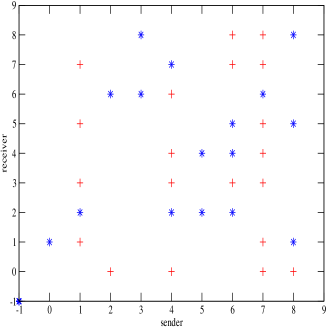
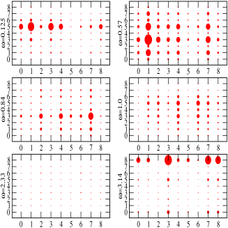
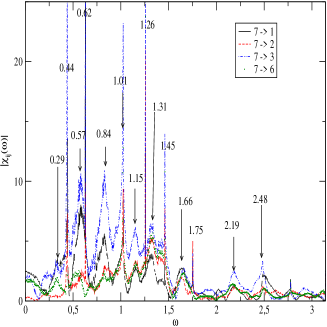
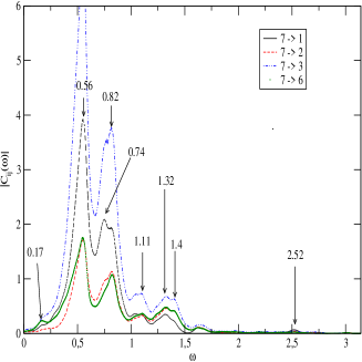
Figure 7: Fig. 7a (left top) Connectivity matrix. Fig. 7b (right top) Modulus of the susceptibilities for all pairs $(i,j)$ and several frequencies $\omega$. The area of the red circle is proportional to the modulus of the susceptibility. Fig. 7c (left bottom) Modulus of the susceptibility for neuron $7$. Fig. 7d. (right bottom) Modulus of the corresponding Fourier transform of the correlations function.

4.3 Conclusion.

The previous analysis leads then us to propose a notion of “effective”, frequency dependent, connectivity based on susceptibility curves. For a given frequency $\omega$, we plot the modulus of the susceptibility $|\chi_{ij}(\omega)|$ with a representation assigning to each pair $i,j$ a circle whose size is proportional to the modulus. We clearly see in figure 7 that changing the frequency changes the effective network.

All these effects are due to a combination of topology and dynamics and they cannot be read in the connectivity matrix ${\cal W}$. Therefore, the example of neural networks treated in this section shows convincingly that the analysis of neural circuits requires a careful investigation of the combined effects induced by non-linear dynamics and topology of the synaptic graph. It also shows that the analysis of correlations provides less information than a linear response analysis. This is particularly clear when looking at the resonances curves displayed by linear response and correlations functions. As we saw, this difference is well understood on theoretical grounds and has deep relations with salient characteristics of the nonlinear dynamics (saturation in the transfer function closely related to the refractory period). Using linear response in neural networks is not new (see for example [145] and references therein), but the point of view adopted in the present section, is, we believe, less known and raises new interesting questions.

For example, one may wander what would bring this approach in spiking neural networks, where the causal action from a neuron to another can be somewhat “directly” read in the timing of pre- and post-synaptic neurons spikes. Another remaining question is what would the use of linear response analysis tell us in neural networks having synaptic plasticity. This issue is briefly addressed in the next section.

5 Dynamical effects of synaptic plasticity

5.1 General context

The notions of neural code and information cannot be separated from the capacity that neuronal networks have to evolve and adapt by plasticity mechanisms, and especially synaptic plasticity. Therefore, understanding the effects of synaptic plasticity on neurons dynamics is a crucial challenge. Especially, addressing the effect of synaptic plasticity in neural networks where dynamics is emerging from collective effects and where spikes statistics are constrained by this dynamics seems to be of central importance. This issue is subject to two main difficulties. On one hand, one must identity the generic dynamical regimes displayed by a neural network model for different choices of parameters (including synaptic weights). Some examples of such analysis have been given in section 2. On the other hand, one must analyse the effects of varying synaptic weights when applying plasticity rules. This requires to handle a complex interwoven evolution where neurons dynamics depends on synapses and synapses evolution depends on neuron dynamics.

Effects of synaptic adaptation

Three main classes of effects can be anticipated [59, 161, 162].

1. Structural effects. There is a first, evident, effect of synaptic plasticity: a rewiring of the neural network. However, this rewiring is not some random process where edges would be selected or removed independently of the history. Instead, it results from a complex process where edges are potentiated or depressed according to the neuron dynamics, which is itself depending on synaptic weights and external stimuli. The question is therefore whether one can nevertheless extract some general characteristics of the network structure evolution and what is the impact of this structure evolution on neural network behaviour.

2. Dynamical effects. Changing the synaptic weights, which are parameters of the dynamical systems (13) and (14), will obviously have an incidence on dynamics. These effects can be smooth or sharp (bifurcations). More generally, one expects period of smooth changes interrupted by sharp transitions (see fig. 8 for an example of this). Thus, adaptation drives the dynamical system along a definite path in the space parameters, which integrates the whole past, via synaptic changes. In this respect, we address a very untypical and complex type of dynamical system. This induces rich properties such as a wide synaptic adaptation-induced variability in the network response to a given stimulus, with the same set of initial synaptic weights, simply by changing the initial conditions.

3. Functional effects. This evolution typically arises when the system is submitted to inputs or stimuli which constrain neuron dynamics and thus synaptic evolution. For simplicity, let us think of synaptic plasticity in the restricted context of “learning” some input. Learning should result in the acquisition of a new ability. The network after learning should be able to “recognise” a learnt input, while this was not necessarily the case before learning. In this context, recognition can be manifested by a drastic change in the dynamics whenever a learnt input is presented. Moreover, this effect must be robust and selective. Examples of this are presented now.

Coupled dynamics

As an illustration we consider now the following coupled dynamics. Neurons are evolving according to (14) (we focus here on discrete time dynamics). We consider slow synapses dynamics. Namely, synaptic weights are constant for $T$ consecutive dynamics steps, where $T$ is large. This defines an “adaptation epoch”. At the end of the adaptation epoch, synaptic weights are updated according to (9). This has the consequence of modifying neurons dynamics and possibly spike trains. The weights are then updated and a new adaptation epoch begins. We denote by $t$ the update index of neuron states (neuron dynamics) inside an adaptation epoch, while $\tau$ indicates the update index of synaptic weights (synaptic plasticity). Call ${\bf X}^{(\tau)}(t)$ the state of the neurons at time $t$ within the adaptation epoch $\tau$ (we use here the notation ${\bf X}$ instead of ${\bf V}$ since eq. (59) holds for model having possibly more variables than the membrane potential for the definition of the neuron state). Let $W_{ij}^{(\tau)}$ be the synaptic weights from neuron $j$ to neuron at $i$ in the $\tau$-th adaptation epoch. At the end of each adaptation epoch, the neuron dynamics indexes are reset, and $X_{i}^{(\tau+1)}(0)=X_{i}^{(\tau)}(T),i=1\dots N$. The coupled dynamics writes:

$$\left\{\begin{array}[]{ccc}{{\bf X}^{(\tau)}(t+1)}&=&{{\bf F}_{\boldsymbol{\gamma}^{(\tau)}}}({{\bf X}^{(\tau)}(t)})\\ \delta W_{ij}^{(\tau)}&\stackrel{{\scriptstyle\rm def}}{{=}}&W_{ij}^{(\tau+1)}-W_{ij}^{(\tau)}=g\left(W_{ij}^{(\tau)},\left[\omega_{i}\right]_{t-T_{s},t},\left[\omega_{j}\right]_{t-T_{s},t})\right)\end{array}\right.$$ (59)

Recall that $\boldsymbol{\gamma}=({\cal W},{\bf{I}}^{(ext)})$ (see section 1.2.4) and $\boldsymbol{\gamma}^{(\tau)}$ is the set of parameters at adaptation epoch $\tau$. In the present setting the external current is used as a time constant external stimulus. We write it $\bm{\xi}$ (see footnote 17).

Let us discuss a few examples.

5.2 Hebbian learning

This example has been considered in [161, 162]. The goal is to study the role of synaptic plasticity mechanisms inspired by Hebb’s work [90] and its generalisation, in a situation where the neural network is submitted to some specific stimulus over a long time. The main is to study the conjugated effects of stimulus action and synaptic plasticity mechanisms on the neural network dynamics. Specifically, we want to investigate whether these conjugated effects can lead the system to a state where it acquires some ability to “recognise” this stimulus. In the example developed below, this corresponds to drive the system, via an Hebb’s-inspired modification of the synaptic weights, in a region in the parameters space where presenting the stimulus induces a bifurcation in the dynamics whereas this bifurcation didn’t occur before synaptic adaptation.

Let us before briefly explain what we mean by “Hebbian learning”. D. Hebb has proposed in [90] a theory of behaviour based on the physiology of the nervous system. The most important concept to emerge from Hebb’s work was his formal statement (known as Hebb’s rule) of how learning could occur.

When an axon of cell A is near enough to excite a cell B and repeatedly or persistently takes part in firing it, some growth process or metabolic change takes place in one or both cells such that A’s efficiency, as one of the cells firing B, is increased.

Many “learning rules” in neural networks are based on Hebb’s observations plus a few well established facts. They rely upon a few recipes that can summarised as [97]:

• Learning results from modifying synaptic connections between neurons.

• Learning is local i.e. the synaptic modification depends only upon the pre- and post- synaptic neurons activity and does not depend upon the activity of the other neurons.

• The modification of synapses is slow compared with characteristic times of neuron dynamics.

• If either pre- or post- synaptic neurons or both are silent then no synaptic change takes place except for (exponential) decay which corresponds to forgetting.

The first item implies that learning results in a modification of the $W_{ij}$’s. The second one basically says that the synaptic modification of $W_{ij}$ writes $W_{ij}^{\prime}=\epsilon h(W_{ij}^{T},m_{j},m_{i})$ where $W_{ij}^{\prime}$ is the value of the synapses $j\to i$ after the learning rule has been applied. The numbers $m_{i}$ ($m_{j}$) denotes the “state” or “activity” of the neuron $i$ ($j$). How this “state” is defined vary according to the model. The third item implies then that $\epsilon$ is a small parameter, whose inverse corresponds to the characteristic time for a significant change of $W_{ij}$. If one assumes that $h$ is a smooth function then one may simply consider a Taylor expansion of a generic regular function $h$. This gives, up to the second order in $m_{i},mj$.

$$W_{ij}^{\prime}=\epsilon\left(a_{000}+a_{100}W_{ij}+a_{010}m_{j}+a_{001}m_{i}+a_{011}m_{i}m_{j}+h.o.t.\right)$$

where h.o.t. means “higher order terms” such as $W_{ij}m_{i}m_{j}$, etc…. Then, the fourth item implies $a_{000}=0$ and leads to introduce a parameter $\lambda=\epsilon a_{100}\in[0,1]$ that models passive “forgetting”: if a synapse is not solicited its intensity decreases with a decay rate $\frac{1}{\lambda}$.

5.2.1 Coupled dynamics.

On these bases, consider the model (32) where synaptic weights evolve according to:

$$W_{ij}^{(\tau+1)}=\lambda W_{ij}^{(\tau)}+\frac{\alpha}{N}\sum_{j=1}^{N}m_{i}^{(\tau)}m_{j}^{(\tau)}H\left[m_{j}^{(\tau)}\right],$$ (60)

where $\alpha$ is a small number, controlling the rate of synaptic plasticity. Here, one associates to the history of neuron $i$’s rate an activity index $m_{i}^{(\tau)}$:

$$m_{i}^{(\tau)}=\frac{1}{T}\sum_{t=1}^{T}(\nu_{i}^{(\tau)}(t)-d_{i})$$

where $\nu_{i}^{(\tau)}(t)$ is the firing rate of neuron $i$ at time $t$ in the adaptation epoch $\tau$, $d_{i}\in[0,1]$ is a threshold. The neuron is considered active during synaptic adaptation epoch $\tau$ whenever $m_{i}^{(\tau)}>0$, and silent otherwise. Finally, $H(x)$ is the Heaviside function.

Let us now interpret this equation. The first term is conform to the recipes introduced in the previous section. The second term is positive whenever neuron $j$ and $i$ are active, increasing the synapse efficacy $W_{ij}$ (i.e. render it more positive if is excitatory and less negative if it is inhibitory). If $j$ is active and $i$ inactive the synapse efficacy decreases. Finally, if $j$ is inactive the second term is zero. We emphasise that this one possible implementation among many others.

Equations (32) & (60) define a dynamical system where two distinct processes (neuron dynamics and synaptic network evolution) interact with distinct time scales. This results in a complex interwoven evolution where neuronal dynamics depends on the synaptic structure and synapses evolve according to neuron activity. On general grounds, this process has a memory that is a priori infinite and the state of the neural network depends on the past history.

5.2.2 Observed effects of Hebbian synaptic plasticity

The effect of this Hebbian synaptic adaptation has been explored numerically in [59] and mathematically in [162]. Assume that the initial synaptic weights are chosen independently, at random, with a Gaussian distribution of mean $\frac{\bar{W}}{N}$ and variance $\frac{\sigma^{2}}{N}$. This choice mimics a situation where no structure is imposed a priori in the correlations between synaptic weights. The idea is to see how synaptic adaptation changes this situation. Then, according to section (2.1.3) dynamics is chaotic provided the gain $g$ of the sigmoid $S$ is large enough. Starting from such a chaotic dynamics, the following effects have been observed, in correspondence with the three effects anticipated in the beginning of this section.

Structural effects.

The rewiring of the network by the synaptic adaptation rule (60) reveals a variation in the synaptic weights distribution, and an increase in weights correlations. This effect is evident but does not give significant hints to interpret the dynamical and functional effects described below [162]. Also, a computation of standard indicators in complex graphs analysis, when applied to the synaptic weights matrix, does not show any salient effect. The only important hint provided by synaptic weights matrix analysis is an increase in the number and weights of positive feedback loops, which renders the system more cooperative, with a strong impact on dynamics [93]. As suggested in the section 4 the analysis of synaptic weights matrix is indeed not expected to provide deep insights on dynamical effects. On the opposite the analysis of Jacobian matrices reveals important properties. This is not surprising. A standard procedure for the analysis of nonlinear dynamical systems starts with a linear analysis. This holds e.g. for stability and bifurcation analysis but also for the computation of indicators such as Lyapunov exponents. The key object for this analysis are Jacobian matrices. Moreover, as we saw in the previous section, Jacobian matrices and their generalisation, the linear response, generate a graph structure that can be interpreted in causal terms.

Dynamical effects.

As a corollary in the increase of positive feedback loops it is observed that Hebbian synaptic adaptation leads to a systematic reduction of the dynamics complexity (transition from chaos to fixed point by an inverse quasi-periodicity route, see fig. 8a). As a corollary the largest Lyapunov exponent $\lambda_{1}^{(\tau)}$, which depends on the synaptic adaptation epoch $\tau$, decreases from positive to negative values. Two main effects contribute to this decay. The first effect is due to passive LTD term in (60). The second one is related to an increase in the level of neurons’ saturation. Basically, cooperativity between neurons has a tendency to either render them more silent, or more active. In both case, this “pushes” them to the saturated part of the sigmoidal transfer function, reducing the average value of $S^{\prime}(V_{i})$. Since the entry $ij$ of the Jacobian matrix, $DF_{ij}({\bf V})=W_{ij}S^{\prime}(V_{i})$ an increase in the saturation of neurons has the effect of decreasing the spectral radius of $D{\bf F}(V)$ with a computable impact on the maximal Lyapunov exponent.

Functional effects.

This property has been exploited for pattern retrieval. Label by ${\bf V}$ the neuron state when the (time constant) input (external current) $\xi$ is applied to the network (see eq. (32)) and by ${\bf V}^{\prime}$ the neuron state without $\xi$. The removal of $\xi$ modifies the attractor structure and the average value of observables. More precisely, let $\phi$ be some suitable function and call:

$$\Delta^{(\tau)}\left[\phi\right]=\left\langle\phi({\bf V}^{\prime})\right\rangle^{(\tau)}-\left\langle\phi({\bf V})\right\rangle^{(\tau)}$$ (61)

where $\left\langle\phi({\bf V}^{\prime})\right\rangle^{(\tau)}$ is the (time or SRB) average value of $\phi$ without $\xi$ and $\left\langle\phi({\bf V})\right\rangle^{(\tau)}$ the average value in the presence of $\xi$. Two cases can arise.

In the first case, the system is away from a bifurcation point and removal results in a variation of $\Delta^{(\tau)}\left[\phi\right]$ that remains proportional to $\xi$, provided $\xi$ is sufficiently small. In the present context, the linear response theory (see section 4) predicts that the variation of the average value of ${\bf V}$ is given by [43, 44]:

$$\Delta^{(\tau)}\left[{\bf V}\right]=-\chi^{(\tau)}\mbox{\boldmath$\xi$}$$ (62)

where

$$\chi^{(\tau)}=\sum_{n=0}^{\infty}\left\langle D{\bf F}^{n}\right\rangle^{(\tau)}$$ (63)

is a matrix whose entries are given by eq. (57) in section 4. Note therefore that $\Delta^{(\tau)}\left[{\bf V}\right]=-\mbox{\boldmath$\xi$}-M^{(\tau)}\mbox{\boldmath$\xi$}$ where the matrix $M^{(\tau)}=\sum_{n=1}^{\infty}\left\langle D{\bf F}^{n}\right\rangle^{(\tau)}$ integrates dynamical effects. The application of $\xi$ implies a reorganisation of the dynamics which results in a complex formula for the variation of $\left\langle{\bf V}\right\rangle^{(\tau)}$, even if the dominant term is $\xi$, as expected. More precisely, as emphasised several times above, one remarks that each path in the sum $\sum_{\gamma_{ij}(n)}$ is weighted by the product of a topological contribution depending only on the weights $W_{ij}$ and on a dynamical contribution. The weight of a path $\gamma_{ij}$ depends on the average value of $\left\langle\prod_{l=1}^{n}f^{\prime}(u_{k_{l-1}}(l-1))\right\rangle^{(\tau)}$ thus on correlations between the state of saturation of the units $k_{0},\dots,k_{n-1}$ at times $0,\dots,n-1$.

In the second case the system is close to a bifurcation point and the presentation/removal of the input induces a sharp variation (bifurcation) in dynamics. In this case, eq. (62) does not apply anymore. We expect therefore input presentation/removal to have a maximal effect close to bifurcations points. This can be revealed by studying the quantity $\Delta^{(\tau)}\left[\phi\right]$ in eq. (61) for the observable $\phi(V_{i})=S^{\prime}(V_{i})$, which measures the level of saturation of neuron $i$ in the state $V_{i}$. Indeed, this quantity is maximal when $V_{i}$ is in the central part of the sigmoidal transfer function, where neuron $i$ is the most sensitive to small variations. Hence this quantity, called $\Delta^{(\tau)}[S^{\prime}]$, measures how neuron excitability is modified when the input is removed. The evolution of $\Delta^{(\tau)}[S^{\prime}]$ during learning following rule eq. (60) is shown on fig. 8b (full lines) for two values of the passive forgetting rate $\lambda$. $\Delta^{(\tau)}[S^{\prime}]$ is found to increase to a maximum at early learning epochs, while it vanishes afterwards. Interestingly, comparison with the decay of the leading eigenvalue $\mu_{1}$ (dotted lines) of the average Jacobian matrix $\left\langle D{\bf F}\right\rangle^{(\tau)}$ shows that the maximal values of $\Delta^{(\tau)}[S^{\prime}]$ are obtained when $|\mu_{1}|$ is close to $1$. This also corresponds to a vanishing of the maximal Lyapunov exponent. Hence, these numerical simulations confirm that sensitivity to input removal is maximal when the leading eigenvalue is close to $1$. Therefore, “Hebb-like” learning drives the global dynamics in a region of the parameters space were sensitivity to the stimulus, manifested by a drastic change in the average of functions hence by a drastic change in the underlying dynamics, is maximal. This property may be crucial regarding memory properties of recurrent neural networks, which must be able to detect, through their collective response, whether a learnt input is present or absent. This property is obtained at the frontier where the strange attractor begins to destabilise ($|\mu_{1}|=1$), hence at the so-called “edge of chaos”.

Note that continuing adaptation after this phase of highest sensitivity, leads to a decay of sensitivity and to a stabilisation of the system to a fixed point (fig. 8a). This is not surprising. Insisting too much on adaptation to this stimulus drive the system to a state where activity pattern is essentially identical to the input, with no room any more for spontaneous activity.

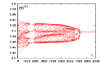
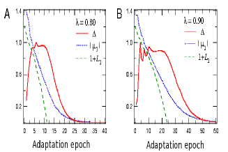
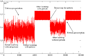
Figure 8: Fig. 8a (left) Inverse quasi periodicity route induced by learning. The plotted quantity is $m^{(\tau)}(t_{0})\stackrel{{\scriptstyle\rm def}}{{=}}\frac{1}{N}\sum_{i=1}^{N}S(V_{i}(t_{0}))$, where $t_{0}\in[0,T]$ is fixed and where the adaptation epoch index $\tau$ varies. Fig. 8b (middle) Sensitivity to the learned input. $\mu_{1}$ is the largest eigenvalue of $\left\langle D{\bf F}\right\rangle^{(\tau)}$ and $L_{1}$ is the largest Lyapunov exponent. Fig. 8c (right) Dynamical effect of input presentation before and after adaptation.

Conclusion.

In fig. 8c we have represented the effect of presenting/removing the input before adaptation, and after adaptation, in the region where the reactivity is maximal. Clearly, the presentation of $\xi$ after adaptation induces a sharp transition in dynamics, which is not occurring before adaptation. Moreover, this effect, inherited via learning, is robust to a small amount of noise, and selective (it does not occur for drastically different patterns) [59]. Though established in the context of a rather simple “neural” model, these results raise interesting questions and comments. They suggest that adaptation corresponds to some path in the space of parameters of (32) leading the system in a region were it acquires sensitivity to the input it has adapted to, this sensitivity being manifested by sharp and rapid variations in neurons dynamics. An obvious question is does this effect generalise to more complex (and realistic) architecture ? This is an ongoing research field.

5.3 Effects of synaptic plasticity on spike trains statistics.

Synaptic plasticity acts also on the statistics of spike trains. Let us now briefly mention recent works where the effects of plasticity on spike train statistics is analysed.

Synapses update as an integration over spikes trains.

Let us reconsider the equation (9) for synaptic weights dynamics. The synaptic variation $\delta W_{ij}$ is the integrated response of the synapse from neuron $j$ to neuron $i$ when neuron $j$ sends a spike sequence $\left[\omega_{j}\right]_{t-T_{s},t}$ and neuron $i$ fires according to $\left[\omega_{i}\right]_{t-T_{s},t}$. This response is not a deterministic function, while (9) is deterministic. As a matter of fact, the explicit form of $g$ is usually derived from phenomenological considerations as well as experimental results where synaptic changes can be induced by specific simulations conditions, defined through the firing frequency of pre- and post-synaptic neurons [23, 64], the membrane potential of the post-synaptic neuron [10], spike timing [119, 124, 19] (see [123] for a review). Thus, these results are usually based on a repetition of experiments involving the excitation of pre- and post-synaptic neurons by specific spike trains. The phenomenological plasticity rules derived from these experiments are therefore of statistical nature. Namely, they do not tell us what will be the exact changes induced on synapses when this or this spike train is applied to pre- and post-synaptic neuron. Instead, they provide us the average synaptic change. Thus, the function $g(W_{ij},\left[\omega_{i}\right]_{t-T_{s},t},\left[\omega_{j}\right]_{t-T_{s},t})$ in (9) is typically a statistical average of the synaptic response when the spike train of neuron $j$ (resp. $i$) is $\left[\omega_{j}\right]_{t-T_{s},t}$ (resp. $\left[\omega_{i}\right]_{t-T_{s},t}$), and the actual synaptic weight value is $W_{ij}$.

Slow synaptic update.

On this basis let us assume that $g$ is obtained via a time average ${\pi_{\omega}^{(T)}}$ (see eq. (47) in section 3) of some function $\phi$ having a form depending on the type of “rule”considered (e.g. Hebbian or STDP). Namely, $g$ has the form:

$$g\left(W_{ij},\left[\omega_{i}\right]_{t-T_{s},t},\left[\omega_{j}\right]_{t-T_{s},t}\right)\equiv\epsilon{\pi_{\omega}^{(T)}}\left[\phi_{ij}(W_{ij},.)\right].$$ (64)

where $\epsilon$ is a parameter that will be typically small. In general $\phi_{ij}$ can be expanded in terms of singlets, pairs, triplets, etc of spikes [77, 40].

Statistical effects of synaptic plasticity

The coupled dynamics (59) has an impact on the set of admissible raster plots and the spikes train statistics. Typically, the empirical average constructed via the raster plot $\omega^{(\tau)}$ in the adaptation epoch $\tau$, changes from ${\pi_{\omega^{(\tau)}}^{(T)}}\to{\pi_{\omega^{(\tau+1)}}^{(T)}}$. Thus, the adaptation dynamics results in a sequence of empirical measures $\left\{{\pi_{\omega^{(\tau)}}^{(T)}}\right\}_{\tau=1}^{\infty}$ and the corresponding statistical model also evolves. Let us characterise this evolution using the tools introduced in section 3. The main idea is to make the assumption that each ${\pi_{\omega^{(\tau)}}^{(T)}}$ can be approximated by a Gibbs measure $\nu_{\boldsymbol{\psi}^{(\tau)}}$ with potential $\boldsymbol{\psi}^{(\tau)}$. Then synaptic adaptation writes:

$$\delta W_{ij}^{(\tau)}=\epsilon\nu_{\boldsymbol{\psi}^{(\tau)}}\left[\phi_{ij}(W_{ij}^{(\tau)},.)\right].$$ (65)

The synaptic update results in a change of parameters $\boldsymbol{\gamma}$, $\boldsymbol{\gamma}^{(\tau+1)}=\boldsymbol{\gamma}^{(\tau)}+\delta\boldsymbol{\gamma}^{(\tau)}$ where $\delta\boldsymbol{\gamma}^{(\tau)}$ is assumed to be small (this is the role of the constant $\epsilon$ in (9)). This induces variation in statistical properties of raster plots (e.g. the topological pressure (48) -see [40] for details). These variations can be smooth or not.

Smooth variations

If they are smooth one can show that there exist a function ${\cal F}^{(\tau)}_{\small{\boldsymbol{\phi}}}({\cal W})$ such that the adaptation rule (65) can be written in the form:

$$\delta{\cal W}^{(\tau)}=\epsilon\nabla_{\tiny{{\cal W}={\cal W}^{(\tau)}}}{\cal F}^{(\tau)}_{\small{\boldsymbol{\phi}}}({\cal W}).$$ (66)

Moreover, this quantity decay under synaptic adaptation. Thus, the adaptation rule (66) is a gradient system where the function ${\cal F}^{(\tau)}_{\small{\boldsymbol{\phi}}}$ decreases when iterating synaptic adaptation rules. Were the transition $\tau\to\tau+1$ to be smooth for all $\tau$, would ${\cal F}^{(\tau)}_{\small{\boldsymbol{\phi}}}$ reach a minimum at some ${\cal W}^{\ast}$ as $\tau\to\infty$. Such a minimum corresponds to $\nabla_{\tiny{{\cal W}^{\ast}}}{\cal F}^{(\tau)}_{\small{\boldsymbol{\phi}}}=0$, thus to

$$\delta W_{ij}^{\ast}={\nu_{\scriptstyle{\boldsymbol{\psi}^{\ast}}}}\left[\phi_{ij}\right]=0,\quad,\forall i,j=1\dots N,$$

according to eq. (66). Hence, this minimum corresponds to a static distribution for the synaptic weights.

Static synaptic weights.

Since this imposes a condition on the average value of the $\phi_{ij}$’s, this imposes as well the statistical model as a Gibbs measure ${\nu_{\scriptstyle{\boldsymbol{\psi}}}}$ with a potential:

$$\boldsymbol{\psi}^{\ast}=\Phi+\boldsymbol{\lambda}^{\ast}.\boldsymbol{\phi},$$ (67)

where $\boldsymbol{\psi}^{\ast}=\left(\psi^{\ast}_{ij}\right)_{i,j=1}^{N}$. The potential $\Phi$ in (67) is such that $\Phi(\omega)=0$ is $\omega$ is admissible and $\Phi(\omega)=-\infty$ if it is forbidden, so that forbidden raster plots have zero probability. We use the notation $\boldsymbol{\phi}=\left(\phi_{ij}\right)_{i,j=1}^{N}$, $\boldsymbol{\lambda}^{\ast}=\left(\lambda^{\ast}_{ij}\right)_{i,j=1}^{N}$ and $\boldsymbol{\lambda}^{\ast}.\boldsymbol{\phi}=\sum_{i,j=1}^{N}\lambda^{\ast}_{ij}\phi_{ij}$. The statistical parameters $\lambda_{ij}^{\ast}$, are given by eq. (50) in section 3.2.

As a conclusion, the statistical model, in the sense of section 3.2, is a Gibbs distribution such that the probability of a spin block $R$ of depth $n$ obeys eq. (52) with a potential $\boldsymbol{\psi}^{\ast}$ (see eq. (71) for an explicit form.)) When this corresponds to the asymptotic state for a synaptic adaptation process, this potential provides us the form of the statistical model after adaptation, and integrates all past changes in the synaptic weights.

Moreover, it has a deep implication. Since the Gibbs distribution obeys the variational principle (48) with ${\nu_{\scriptstyle{\boldsymbol{\psi}^{\ast}}}}[\boldsymbol{\phi}]=0$ , the probability distribution ${\nu_{\scriptstyle{\boldsymbol{\psi}^{\ast}}}}$ has maximal entropy. In other words, synaptic adaptation rules of type (65), when they converge, drive the system toward a dynamics where the statistical entropy of spike train is maximal, taking into account the constraints imposed by dynamics.

Singular variations.

The synaptic weights variations can induce a change in the set of admissible raster plots that the system is able to display. When this happens the set of admissible raster plots is suddenly modified by the synaptic adaptation mechanism. Formerly forbidden sequences become allowed, formerly allowed sequences become forbidden, but also a large core of legal sequences may remain legal. These changes depend obviously on the detailed form of neuron dynamics (14) and of the synaptic update mechanism (9). An interesting situation occurs when the set of admissible raster plots obtained after adaptation belongs to $\Sigma_{\boldsymbol{\gamma}^{(\tau)}}\cap\Sigma_{\boldsymbol{\gamma}^{(\tau+1)}}$. In this case, adaptation plays the role of a selective mechanism where the set of admissible raster plots, viewed as a neural code, is gradually reducing, producing after $n$ steps of adaptation a set $\cap_{m=1}^{n}\Sigma_{\boldsymbol{\gamma}^{(m)}}$ which can be rather small. If we consider the situation where (14) is a neural network submitted to some stimulus, where a raster plot $\omega$ encodes the spike response to the stimulus, then $\Sigma_{\boldsymbol{\gamma}}$ is the set of all possible raster plots encoding this stimulus. Adaptation results in a reduction of the possible coding, thus reducing the variability in the possible responses.

Example: Spike Time Dependent Plasticity.

As an example we consider a neural network of type (41) with an adaptation rule inspired from (11) with an additional term $r_{d}W_{ij}^{(\tau)}$, $-1<r_{d}<0$, corresponding to passive LTD.

$$\delta W_{ij}^{(\tau)}=\epsilon\left[r_{d}W_{ij}^{(\tau)}+\frac{1}{T}\sum_{t=T_{s}}^{T+T_{s}}\omega_{j}^{(\tau)}(t)\sum_{u=-T_{s}}^{T_{s}}f(u)\,\omega_{i}^{(\tau)}(t+u)\right],$$ (68)

where $f(x)$ is given by (12) and with:

$$T_{s}\stackrel{{\scriptstyle\rm def}}{{=}}2\max(\tau_{+},\tau_{-}).$$

Set :

$$\phi_{ij}(W_{ij},\omega)=r_{d}W_{ij}+\omega_{j}(0)\sum_{u=-T_{s}}^{T_{s}}f(u)\,\omega_{i}(u),$$ (69)

then (68) has the form (64), $\delta W_{ij}^{(\tau)}=\epsilon{\pi_{\omega^{(\tau)}}^{(T)}}\left[\phi_{ij}(W_{ij},.)\right]$.

Static weights.

Thanks to the soft bound term $r_{d}W_{ij}$ the synaptic adaptation rule admits a static solution given by:

$$W_{ij}=-\frac{\sum_{u=-T_{s}}^{T_{s}}f(u){\pi_{\omega^{(\tau)}}^{(T)}}\left[\omega_{j}(0)\omega_{i}(u)\right]}{r_{d}}.$$ (70)

The sign of $W_{ij}$ depend on the parameters $A_{-},A_{+},T_{s}$, but also on the relative strength of the terms ${\pi_{\omega^{(\tau)}}^{(T)}}\left[\omega_{j}(0)\,\omega_{i}(u)\right]$. Note that this equation may have several solutions.

Spike train statistics in a static weights regime.

As emphasised in section 3.2 and 5.3, when the synaptic adaptation rule converges to a fixed point, the corresponding statistical model is a Gibbs measure with a potential

$$\boldsymbol{\psi}^{\ast}=\Phi+\sum_{i=1}^{N}\sum_{j=1}^{N}\lambda^{\ast}_{ij}\phi_{ij},$$

where the value $\lambda_{ij}^{\ast}$ of the Lagrange multipliers is constrained by the relation (70). Henceforth, the probability of an admissible spike bloc $R$ is given by:

$$P\left[R|S\right]=\frac{1}{Z_{n}\left[\lambda^{\ast}_{1,1}(S),\dots,\lambda^{\ast}_{N,N}(S)\right]}\exp\left[\sum_{i=1}^{N}\sum_{j=1}^{N}\lambda^{\ast}_{ij}(S)\sum_{t=0}^{n-1}\sum_{u=-T_{s}}^{T_{s}}f(u)\omega_{j}(t)\omega_{i}(u+t)\right].$$ (71)

Note that the term $r_{d}W_{ij}$ arising in the definition of the potential can be removed thanks to the normalisation constant $Z_{n}\left[\lambda_{1}(S),\dots,\lambda_{l}(S)\right]$.

Conclusion

At the end of section 3 we were asking whether it is possible to propose a canonical form for spike trains statistical models relying on some generic principle ? Here, we have exhibited an example where such a construction can be made. Our argumentation suggests that Gibbs measures may be good statistical models for a neuron dynamics resulting from slow adaptation rules where synaptic weights converge to a fix value. In this case, synaptic weights contains the whole history of the neural network, expressed in the structure of the generating function of cumulants (the topological pressure) and in the structure of allowed/forbidden raster plots (potential $\Phi$ in (67)). This theoretical results, confirmed by numerical experiments [40], can be compared with the recent paper of Schneidman and collaborators, already quoted in section 3, proposing a Gibbs distribution with Ising like potential to match empirical data on the salamander retina [155]. Our approach suggests that Gibbs distribution could be ubiquitous and that the corresponding potential can be inferred according to the plasticity mechanisms at work, defining the “rule”.

6 Conclusion

In this paper we have presented a series of results related to questions, that, we believe, are central in the computational neuroscience community. These questions, when addressed from the point of dynamical systems theory, shed new light on neural network dynamics with possible outcomes towards experimentation. Interestingly enough, the tools and concepts used here however are not restricted to the field of neural networks but could be applied to other type of “complex” systems.

We now would like now to point out some “challenging” points raised in this paper, which, to our opinion, are central at the current state of the art, in the neuroscience community, especially for those people who want to use models and their analysis to “understand some fundamental keys ruling the behaviour of neural networks”. We also believe that some of these questions address also to experimentalists community.

Finite size corrections.

When dealing with large populations of networks, theoretical methods such as mean-field approaches, neural mass models, large deviations, use a limit $N\to\infty$ where $N$ is the number of neurons. When dealing with “concrete” neural systems the number is finite and finite size systems can have a behaviour that departs strongly from the limiting system. Computing these finite size corrections is an open problem in the whole scientific community (not only neuroscience).

Finite time corrections.

A similar question holds for finite time effects. While many theoretical methods assume stationarity in the data, concrete experiments handle non stationary or transient dynamics. There exists currently empirical methods to tackle this problem such as sliding time windows. But, to the best of our knowledge there are rather few methods (i) to estimate the width of this window which must be large enough to ensure reliable statistical estimates and smaller than relevant characteristic time scales of the non-stationary dynamics; (ii) to define a priori the statistical models (resp. the set of observable) used to characterize dynamics; (iii) to propose and compute reliable indicators that guarantee the liability of the result.

Correlated weights.

Synaptic weights are non independent in real neuronal networks since e.g. plasticity build correlations, that can have long range in space and time. How to characterize these correlations ? How to measure them ? How to handle them in a model ? For example, the mean-field approaches developed in section 2.1 cannot be extended in a straightforward way to this case. Here again there is a need to invent new theoretical methods. Promising results using spectral properties of graphs [108, 12, 107, 6, 22] combined to such linear responses methods as developed in section 4 could provide a breakthrough.

Continuous time.

Most phenomenological models of neurons, such as Hodgkin-Huxley’s, use a description with ordinary differential equations assuming a continuous time. This comes from the description of neurons in terms of membrane potential, a notion which corresponds to an integration over space $dx$ and time scale $dt$ where classical equations of electrodynamics holds (Kirchhoff and Ohm’s law). Also, as we saw, Hodgkin-Huxley’s equations for example, corresponds to integrating the activity of ionic channel at space and time scales so that the notion of probability of open/closed channel have a meaning and, moreover, so that the Markovian approach used for the master equations (2,3,4,) in section 1.2 holds. In other words, writing neurons dynamics at the scale of ionic channel would requires the use of a different physics. Though this remarks looks obvious it prevents one to take the continuum limits $dx\to 0$ or $dt\to 0$ without caution. On the opposite, the “spike” description of neurons is discrete and assume a time discretisation $\delta$ (see section 1.2) such that a given neuron can produce, at most, one spike within this time delay. This time discretisation is essential for the definition of raster plots, as we saw. The existence of a minimal time scale $\delta$ can be defended using arguments from physics and neuronal characterisation (see [45]). However, time discretisation as done in section 1.2 for the definition of raster plots, imposes a time grid which can be contested as well since one may argue that a neuron spike can occur at “any” time (with the restriction discussed above on “continuous” time) while the time grid set it to a time multiple of $\delta$ [114]. So, a central question is: does the effects induced by this slight error on a spike time matters ? This question can be addressed in the realm of models (like gIF models) and the answer is: “it depends”. Indeed, according to the control parameters values such an error can be damped (then it is harmless) or amplified by dynamics. This is precisely the discussion on contraction and initial conditions sensitivity presented in section 2.2.3. Here, the mathematical analysis relies strongly on the simple structure of IF models. But the question of time discretisation and “How precise is the timing of action potentials” [114] must be certainly addressed in a more general context and for more general models.

Neural code and predictability

Another interesting issue, raised by the dynamical system point of view is the following. When building models which reproduce the dynamics of neural assemblies, one is faced to the question “how well does this model approximate real neural systems”. Let us state in a different way. Assume that we have built some artificial neural network that mimics some part of the brain and assume (Gedanken experiment) that we are able to remove this part of the brain and to replace it by our artificial system, what do we need to ensure that this ”cyborg brain” works “as” the original one ? This is a (too) wide open question but let us focus the discussion on “spikes” aspects for simplicity. Our artificial system receives spikes from other parts of the brain and respond with spikes trains that it sends to various brain areas. Must this device be able to reproduce exactly, spikes par spikes, the response of the piece of brain that it replaces ? It is possible to reproduce exactly the response of one neuron to Poisson stimuli [106], and also at the level of a network, to reproduce exactly finite spike trains coming from biological neurons over a finite time [147]. But, from the dynamical system point of view this appears to be too restrictive since, as we saw, in many cases dynamics is chaotic. If one jitters the time of a single spike, the output of the network can change dramatically. Thus this property is not robust and reliable. So which characteristics of the spike train must be reproduced ? This question seems a clear challenge for a not so near future. This also raise questions such as: Are all details important in modelling neural networks ? Which details can be neglected and what is imposed by the biological structure ?

Though the analysis presented here is rather simple compared to the overwhelming richness of brain dynamics, we hope that this work will be useful for readers interested in this beautiful ongoing research field, computational neuroscience.

References

- [1] L. Abbott and C. Van Vreeswijk. Asynchronous states in networks of pulse-coupled neuron. Phys. Rev, 48:1483–1490, 1993.
- [2] M. Abeles. Local Cortical Circuits: An Electrophysiological study. Springer, Berlin, 1982.
- [3] M. Abeles. Corticonics: Neural Circuits of the Cerebral Cortex. Cambridge University Press., New-York, 1991.
- [4] M. Abeles, E. Vaadia, H. Bergman, Y. Prut, I. Haalman, and H. Slovin. Dynamics of neuronal interactions in the frontal cortex of behaving monkeys. Concepts in Neuroscience, 4:131–158, 1993.
- [5] E. Adrian and Y. Zotterman. The impulses produced by sensory nerve endings: Part ii: The response of a single end organ. J Physiol (Lond.), 61:151–71, 1926.
- [6] V. Afraimovich and L. A. Bunimovich. Dyamical networks: interplay of topology, interactions and local dynamics. Nonlinearity, 20:1761–1777, 2007.
- [7] S. Amari. Characteristics of random nets of analog neuron-like elements. Syst. Man Cybernet. SMC-2, 1972.
- [8] S.-I. Amari, K. Yoshida, and K.-I. Kanatani. A mathematical foundation for statistical neurodynamics. Siam J. Appl. Math., 33(1):95–126, 1977.
- [9] E. Arabzadeh, S. Panzeri, and M. Diamond. Deciphering the spike train of a sensory neuron: Counts and temporal patterns in the rat whisker pathway. The Journal of Neuroscience, 26(36):9216–9226, 2006.
- [10] A. Artola, S. Bröcher, and W. Singer. Different voltage-dependent thresholds for inducing long-term depression and long-term potentiation in slices of rat visual cortex. Nature, 347(6288):69–72, 1990.
- [11] P. Ashwin and M. Timme. Unstable attractors: existence and robustness in networks of oscillators with delayed pulse coupling. Nonlinearity, 18:2035–2060, 2005.
- [12] F. M. Atay, T. Biyikoglu, and J. Jost. Network synchronization: Spectral versus statistical properties. Physica D, 224:35–41, 2006.
- [13] M. Barahona and L. Pecora. Synchronization in small-world systems. Phys. Rev. Lett., 89:054101, 2002.
- [14] R. Barbieri, L. M. Frank, D. P. Nguyen, M. C. Quirk, M. A. Wilson, and E. N. Brown. Dynamic analyses of information encoding in neural ensembles. Neural Computation, 16:277–307, 2004.
- [15] R. Barjavel. La voyageur imprudent. folio, 1944.
- [16] G. Ben-Arous and A. Guionnet. Large deviations for Langevin spin glass dynamics. Probability Theory and Related Fields, 102(4):455–509, 1995.
- [17] G. Ben-Arous and A. Guionnet. Symmetric Langevin Spin Glass Dynamics. The Annals of Probability, 25(3):1367–1422, 1997.
- [18] G. BenArous and A. Guionnet. Large deviations for langevin spin glass dynamics. Probability Theory and Related Fields, 102:455–509, 1995.
- [19] G. Bi and M. Poo. Synaptic modification by correlated activity: Hebb’s postulate revisited. Annual Review of Neuroscience, 24:139–166, 2001.
- [20] E. L. Bienenstock, L. Cooper, and P. Munroe. Theory for the development of neuron selectivity: orientation specificity and binocular interaction in visual cortex. The Journal of Neuroscience, 2(1):32––48, 1982.
- [21] P. Blanchard, B. Cessac, and T. Krueger. What can one learn about self-organized criticality from dynamical system theory ? Journal of Statistical Physics, 98:375–404, 2000.
- [22] P. Blanchard and D. Volchenkov. Mathematical Analysis of Urban Spatial Networks. understanding complex systems. Springer Verlag, 2009.
- [23] T. Bliss and A. Gardner-Medwin. Long-lasting potentiation of synaptic transmission in the dentate area of the unanaesthetised rabbit following stimulation of the perforant path. J Physiol, 232:357–374, 1973.
- [24] S. Boccaletti, V. Latora, Y. Moreno, M. Chavez, and D. U. Hwang. Complex networks : Structure and dynamics. Physics Reports, 424:175–308, 2006.
- [25] R. Bowen. Equilibrium states and the ergodic theory of Anosov diffeomorphisms, volume 470 of Lect. Notes.in Math. Springer-Verlag, New York, 1975.
- [26] R. Bowen. Equilibrium states and the ergodic theory of Anosov diffeomorphisms. Second revised version., volume 470 of Lect. Notes.in Math. Springer-Verlag, 2008.
- [27] P. C. Bressloff and P. S. Coombes. A dynamical theory of spike train transitions in networks of integrate-and-fire oscillators. SIAM J Appl Math, 60:820–841, 2000.
- [28] P. C. Bressloff and P. S. Coombes. Dynamics of strongly coupled spiking neurons. Neural Computation, 12(1):91–129, 2000.
- [29] P. C. Bressloff and S. Coombes. Synchronization of synaptically-coupled neural oscillators in: Epilepsy as a dynamic disease, chapter 7. J.Milton and P. Jung, Springer-Verlag, 2003.
- [30] R. Brette and W. Gerstner. Adaptive exponential integrate-and-fire model as an effective description of neuronal activity. Journal of Neurophysiology, 94:3637–3642, 2005.
- [31] R. Brette, M. Rudolph, T. Carnevale, M. Hines, D. Beeman, J. M. Bower, M. Diesmann, A. Morrison, P. H. Goodman, F. C. H. Jr., M. Zirpe, T. Natschläger, D. Pecevski, B. Ermentrout, M. Djurfeldt, A. Lansner, O. Rochel, T. Vieville, E. Muller, A. P. Davison, S. E. Boustani, and A. Destexhe. Simulation of networks of spiking neurons: a review of tools and strategies. Journal of Computational Neuroscience, 23(3):349–398, 2007.
- [32] N. Brunel and V. Hakim. Fast global oscillations in networks of integrate-and-fire neurons with low firing rates. Neural Computation, 11:1621–1671, 1999.
- [33] N. Brunel and P. Latham. Firing rate of noisy quadratic integrate-and-fire neurons. Neural Computation, 15:2281–2306, 2003.
- [34] N. Brunel and S. Sergi. Firing frequency of leaky integrate and fire neurons with synaptic current dynamics. J. Theor. Biol., 195(87–95), 1998.
- [35] B. Cessac. Occurence of chaos and at line in random neural networks. Europhys. Lett., 26(8):577–582, 1994.
- [36] B. Cessac. Increase in complexity in random neural networks. Journal de Physique I (France), 5:409–432, 1995.
- [37] B. Cessac. Does the complex susceptibility of the hénon map have a pole in the upper-half plane ? a numerical investigation. Nonlinearity, 20:2883–2895, 2007.
- [38] B. Cessac. A discrete time neural network model with spiking neurons. rigorous results on the spontaneous dynamics. J. Math. Biol., 56(3):311–345, 2008.
- [39] B. Cessac, B. Doyon, M. Quoy, and M. Samuelides. Mean-field equations, bifurcation map, and route to chaos in discrete time neural networks. Physica 74 D, pages 24–44, 1994.
- [40] B. Cessac, H.Rostro-Gonzalez, J. Vasquez, and T. Viéville. How gibbs distribution may naturally arise from synaptic adaptation mechanisms: a model based argumentation. to appear in J. Stat. Phys, 2009.
- [41] B. Cessac and M. Samuelides. From neuron to neural networks dynamics. EPJ Special topics: Topics in Dynamical Neural Networks, 142(1):7–88, 2007.
- [42] B. Cessac and J. Sepulchre. Stable resonances and signal propagation in a chaotic network of coupled units. Phys. Rev. E, 70(056111), 2004.
- [43] B. Cessac and J. Sepulchre. Transmitting a signal by amplitude modulation in a chaotic network. Chaos, 16(013104), 2006.
- [44] B. Cessac and J. Sepulchre. Linear response in a class of simple systems far from equilibrium. Physica D, 225(1):13–28, 2007.
- [45] B. Cessac and T. Viéville. On dynamics of integrate-and-fire neural networks with adaptive conductances. Frontiers in neuroscience, 2(2), jul 2008.
- [46] J. Chazottes, E. Floriani, and R. Lima. Relative entropy and identification of gibbs measures in dynamical systems. J. Statist. Phys., 90(3-4):697–725, 1998.
- [47] J. Chazottes and G. Keller. Pressure and Equilibrium States in Ergodic Theory, chapter Ergodic Theory. Encyclopedia of Complexity and System Science, Springer, 2009. to appear.
- [48] A. V. Chizhov and L. J. Graham. Population model of hippocampal pyramidal neurons, linking to refractory density approach to conductance-based neurons. Phys. rev. E, 75(011924):114, 2007.
- [49] C. C. Chow and N. Kopell. Dynamics of spiking neurons with electrical coupling. Neural Computation, 12:1643–1678, 2000.
- [50] S. Coombes. Liapunov exponents and mode-locked solutions for integrate-and-fire dynamical systems. Physics Letters A, 255:49–57, 1999.
- [51] S. Coombes and P. C. Bressloff. Mode-locking and arnold tongues in integrate-and-fire neural oscillators. Physical Review E, 60:2086–2096, 1999.
- [52] L. Cooper, N. Intrator, B. Blais, and H. Shouval. Theory of cortical plasticity. World Scientific, Singapore, 2004.
- [53] D. Cosandier-Rimélé, J. Badier, P. Chauvel, and F. Wendling. A physiologically plausible spatio-temporal model for EEG signals recorded with intracerebral electrodes in human partial epilepsy. IEEE Transactions on Biomedical Engineering, 54(3):380–388, 2007.
- [54] M. Cosnard and J. Demongeot. On the definitions of attractors, volume 1163(23). Springer Lecture Notes in Mathematics, 1985.
- [55] M. Cosnard, J. Demongeot, K. Lausberg, and K. Lott. Mathematics applied to biology and medicine, chapter Attractors, Confiners and fractal dimensions: applications in neuromodelling. Wuerz publishing Ltd, 1993.
- [56] A. Crisanti and H. Sompolinsky. Dynamics of spin systems with randomly asymmetric bonds: Langevin dynamics and a spherical model. Physical Review A, 36(10):4922–4939, 1987.
- [57] A. Crisanti and H. Sompolinsky. Dynamics of spin systems with randomly asymmetric bounds: Ising spins and glauber dynamics. Phys. Review A, 37(12):4865, 1987.
- [58] J. Cronin. Mathematical aspects of Hodgkin-Huxley theory. Cambridge University Press, 1987.
- [59] E. Daucé, M. Quoy, B. Cessac, B. Doyon, and M. Samuelides. Self-organization and dynamics reduction in recurrent networks: stimulus presentation and learning. Neural Networks, 11:521–33, 1998.
- [60] P. Dayan and L. F. Abbott. Theoretical Neuroscience : Computational and Mathematical Modeling of Neural Systems. MIT Press, 2001.
- [61] J. R. L. De Almeida and D. J. Thouless. Stability of the sherrington-kirkpatrick solution of a spin glass model. Journal of Physics A: Mathematical and General, 11(5):983–990, 1978.
- [62] A. Delorme, L. Perrinet, and S. Thorpe. Networks of integrate-and-fire neurons using rank order coding b: Spike timing dependent plasticity and emergence of orientation selectivity. Neurocomputing, 38-40:539–45, 2001.
- [63] M. Diesmann, M.-O. Gewaltig, and A. Aertsen. Stable propagation of synchronous spiking in cortical neural networks. Nature, 402:529–533, 1999.
- [64] S. Dudek and M. F. Bear. Bidirectional long-term modification of synaptic effectiveness in the adult and immature hippocampus. J Neurosci., 13(7):2910–2918, 1993.
- [65] J.-P. Eckmann and D. Ruelle. Ergodic Theory of Chaos and Stange Attractors. Review of Modern Physics, 57(3):617–656, 1985.
- [66] B. Ermentrout. Neural networks as spatio-temporal pattern-forming systems. Reports on Progress in Physics, 61:353–430, 1998.
- [67] G. Ermentrout and N. Koppel. Frequency plateaus in a chain of weakly coupled oscillators. SIAM J. Math. Anal., 15:215–23, 1984.
- [68] U. Ernst, K. Pawelzik, and T. Geisel. Synchronization induced by temporal delays in pulse-coupled oscillators. Phys. Rev. Lett., 74(9):1570–1573, 1995.
- [69] O. Faugeras, J. Touboul, and B. Cessac. A constructive mean field analysis of multi population neural networks with random synaptic weights and stochastic inputs. Frontiers in Neuroscience, 2008. submitted.
- [70] R. Fitzhugh. Theoretical Effect of Temperature on Threshold in the Hodgkin-Huxley Nerve Model. The Journal of General Physiology, 49(5):989–1005, 1966.
- [71] N. Fourcaud and N. Brunel. Dynamics of the firing probability of noisy integrate-and-fire neurons. Neural Computation, 14:2057–2110, 2002.
- [72] N. Fourcaud-Trocme, D. Hansel, C. van Vreeswijk, and N. Brunel. How Spike Generation Mechanisms Determine the Neuronal Response to Fluctuating Inputs. Journal of Neuroscience, 23(37):11628, 2003.
- [73] J. Gambaudo and C. Tresser. Le chaos, théorie et expériences. Collection CEA, 1988.
- [74] Y. Gao, I. Kontoyiannis, and E. Bienenstock. Estimating the entropy of binary time series: Methodology, some theory and a simulation study. Entropy, 10(2):71–99, 2008.
- [75] W. Gerstner. Time structure of the activity in neural network models. Physical Review E, 51(1):738–758, 1995.
- [76] W. Gerstner and W. Kistler. Spiking Neuron Models. Cambridge University Press, 2002.
- [77] W. Gerstner and W. M. Kistler. Mathematical formulations of hebbian learning. Biological Cybernetics, 87:404–415, 2002.
- [78] V. Girko. Circular law. Theor. Prob. Appl, 29:694–706, 1984.
- [79] P. Gong and C. van Leeuwen. Dynamically maintained spike timing sequences in networks of pulse-coupled oscillators with delays. Phys. Rev. Lett, 98(048104), 2007.
- [80] F. Grammont and A. Riehle. Precise spike synchronization in monkey motor cortex involved in preparation for movement. Exp. Brain Res., 128:118–122, 1999.
- [81] F. Grimbert. Mesoscopic models of cortical structures. PhD thesis, University of Nice Sophia-Antipolis, feb 2008.
- [82] F. Grimbert and O. Faugeras. Analysis of jansen’s model of a single cortical column. Technical Report RR-5597, INRIA, June 2005.
- [83] G. Grinstein and R. Linsker. Synchronous neural activity in scale-free network models versus random network models. PNAS, 28(102):9948–9953, 2005.
- [84] J. Guckenheimer and I. S. Labouriau. Bifurcation of the hodgkin-huxley equations: A new twist. Bull. Math. Biol., 55:937–952, 1993.
- [85] J. Guckenheimer and R. Oliva. Chaos in the hodgkin–huxley model. SIAM Journal on Applied Dynamical Systems, 1:105, 2002.
- [86] A. Guionnet. Averaged and quenched propagation of chaos for spin glass dynamics. Probability Theory and Related Fields, 109(2):183–215, 1997.
- [87] M. M. Gupta, L. Jin, and N. Homma. Static and dynamic neural networks: from fundamentals to advanced theory. Wiley-IEEE, 2003.
- [88] D. Hansel, G. Mato, C. Meunier, and L. Neltner. On numerical simulations of integrate-and-fire neural networks. Neural Computation, 10:467–483, 1998.
- [89] H. Hasegawa. Synchronisations in small-world networks of spiking neurons : Diffusive versus sigmoid couplings. Phys. Rev. E., 72:056139, 2005.
- [90] D. Hebb. The organization of behavior: a neuropsychological theory. Wiley, NY, 1949.
- [91] J. Hertz. Theoretical Aspects of Neural Computation., chapter Modelling synfire processing., pages 135–144. Wong K-Y M. King I. and Yeung D-Y (eds), Springer-Verlag, 1997.
- [92] B. Hille. Ion channels of excitable membranes. Sinauer Sunderland, Mass, 2001.
- [93] M. Hirsch. Convergent activation dynamics in continuous time networks. Neur. Networks, 2:331–349, 1989.
- [94] A. Hodgkin and A. Huxley. A quantitative description of membrane current and its application to conduction and excitation in nerve. Journal of Physiology, 117:500–544, 1952.
- [95] H. Hong, B. Kim, M. Choi, and H. Park. Factors that predict better synchronizability on complex networks. Phys. Rev. E, 65:067105, 2002.
- [96] F. Hoppenstaedt and E. Izhikevich. Weakly Connected Neural Networks. Springer-Verlag, New York, 1997.
- [97] F. Hoppensteadt and E. Izhikevich. Weakly connected neural networks. Springer-Verlag New York, Inc., 1997.
- [98] B. R. Hunt, T. Sauer, and J. A. Yorke. Prevalence: A translation-invariant ‘almost every’ on infinite-dimensional spaces. Bull. Am. Math. Soc., 27:217–238, 1992.
- [99] E. Izhikevich. Which model to use for cortical spiking neurons? IEEE Trans Neural Netw, 15(5):1063–1070, September 2004.
- [100] E. Izhikevich and N. Desai. Relating stdp to bcm. Neural Computation, 15:1511–1523, 2003.
- [101] S. Jahnke, R.-M. Memmesheimer, and M. Timme. Stable irregular dynamics in complex neural networks. Phys. Rev. Lett., 100, 2008.
- [102] B. H. Jansen and V. G. Rit. Electroencephalogram and visual evoked potential generation in a mathematical model of coupled cortical columns. Biological Cybernetics, 73:357–366, 1995.
- [103] E. Jaynes. Information theory and statistical mechanics. Phys. Rev., 106:620, 1957.
- [104] D. Johnson. Neural population structure and consequences for neural coding. Journal of Computational Neuroscience, 16(1):69–80, 2004.
- [105] K. O. Johnson. Sensory discrimination: neural processes preceding discrimination decision. J Neurophysiol, 43(6):1793–1815, 1980.
- [106] R. Jolivet, A. Rauch, H.-R. Lescher, and W. Gerstner. ”Integrate-and-Fire models with adaptation are good enough”. MIT Press, Cambridge, 2006.
- [107] J. Jost, S. Jalan, and F. M. Atay. Detecting global properties of coupled dynamics using local symbolic dynamics. Chaos, 16(033124):1–9, 2006.
- [108] J. Jost and M. P. Joy. Spectral properties and synchronization in coupled map lattices. Phys. Rev. E, 65:016201–1–9, 2002.
- [109] A. Katok and B. Hasselblatt. Introduction to the modern theory of dynamical systems. Kluwer, 1998.
- [110] J. Keener, F. Hoppensteadt, and J. Rinzel. Integrate-and-fire models of nerve membrane response to oscillatory input. SIAM Journal of Applied Mathematics, 41(3):503–517, 1981.
- [111] J. Keener and J. Sneyd. Mathematical Physiology, volume 8 of Interdisciplinary Applied Mathematics. Springer, New York, 1998.
- [112] G. Keller. Equilibrium States in Ergodic Theory. Cambridge University Press, 1998.
- [113] C. Kirst, T. Geisel, and M. Timme. Sequential desynchronization in networks of spiking neurons with partial reset. Phys. Rev. Lett., 102(068101), 2009.
- [114] C. Kirst and M. Timme. How precise is the timing of action potentials. Front. Neurosci., 3(1):2–3, 2009.
- [115] B. W. Knight. Dynamics of encoding in a population of neurons. J. Gen. Physiol., 59:734–766, 1972.
- [116] C. Koch. Biophysics of Computation: Information Processing in Single Neurons. Oxford University Press: New York., 1999.
- [117] L. F. Lago-Fernández, R. Huerta, F. Corbacho, and J. A. Sigüenza. Fast response and temporal coherent oscillations in small-world networks. Phys. Rev. Lett., 84:2758–2761, 200.
- [118] L. Lapicque. Recherches quantitatifs sur l’excitation des nerfs traitee comme une polarisation. J. Physiol. Paris, 9:620–635, 1907.
- [119] W. Levy and D. Stewart. Temporal contiguity requirements for long-term associative potentiation/depression in the hippocampus. Neuroscience, 8(4):791––797, 1983.
- [120] V. Litvak, H. Sompolinsky, I. Segev, and M. Abeles. On the transmission of rate code in long feedforward networks with excitatory-inhibitory balance. Journal of Neuroscience, 23(7):3006–3015, 2003.
- [121] R. Mackay and C. Tresser. Transition to topological chaos for circle maps. Physica D, 19(2):206–273, 1986.
- [122] S. Mahon, G. Casassus, C. Mulle, and S. Charpier. Spike-dependent intrinsic plasticity increases firing probability in rat striatal neurons in vivo. J Physiol., 1(550 (Pt 3)):947–59, 2003.
- [123] R. C. Malenka and R. A. Nicoll. Long-term potentiation - a decade of progress ? Science, 285(5435):1870 – 1874, 1999.
- [124] H. Markram, J. Lübke, M. Frotscher, and B. Sakmann. Regulation of synaptic efficacy by coincidence of postsynaptic ap and epsp. Science, 275(213), 1997.
- [125] M. Mattia and P. Del Giudice. Population dynamics of interacting spiking neurons. Physical Review E, 66(5):51917, 2002.
- [126] R.-M. Memmesheimer and M. Timme. Designing complex networks. Phys. Rev. Lett., 224:182–201, 2006.
- [127] M. Mézard, G. Parisi, and M. Virasoro. Spin-glass theory and beyond. World scientific Singapore, 1987.
- [128] K. Miller, J. Keller, and M. Stryker. Ocular dominance column development: analysis and simulation. Science, 245(4918):605–615, 1989.
- [129] J. Milnor. On the concept of attractor. Comm. Math. Phys., 99:177, 1985.
- [130] R. E. Mirollo and S. H. Strogatz. Synchronization of pulse-coupled biological oscillators. SIAM J. Appl. Math., 50:1645–1662, 1990.
- [131] L. Molgedey, J. Schuchardt, and H. Schuster. Supressing chaos in neural networks by noise. Physical Review Letters, 69(26):3717–3719, 1992.
- [132] O. Moynot and M. Samuelides. Large deviations and mean-field theory for asymmetric random recurrent neural networks. Probability Theory and Related Fields, 123(1):41–75, 2002.
- [133] J. Nagumo, S. Arimoto, and S. Yoshizawa. An active pulse transmission line simulating nerve axon. Proc.IRE, 50:2061–2070, 1962.
- [134] M. Nelson and J. Rinzel. The Hodgkin-Huxley model., chapter 4, pages 27–51. Bower and Beeman. The book of Genesis. Springer, New York, 1995.
- [135] I. Nemenman, G. Lewen, W. Bialek, and R. de Ruyter van Steveninck. Neural coding of a natural stimulus ensemble: Information at sub-millisecond resolution. PLoS Comp Bio, 4:e1000025, 2006.
- [136] S. Nirenberg and P. Latham. Decoding neuronal spike trains: how important are correlations. Proceeding of the Natural Academy of Science, 100(12):7348–7353, 2003.
- [137] T. Nishikawa, A. E. Motter, Y. C. Lai, and F. C. Hoppensteadt. Heterogeneity in oscillator networks : are smaller worlds easier to synchronize ? Phys. Rev. Lett., 91, 2003.
- [138] L. Osbone, S. Palmer, S. Lisberger, and W. Bialek. Combinatorial coding in neural populations. arXiv.org:0803.3837, 2008.
- [139] W. Parry and M. Pollicott. Zeta functions and the periodic orbit structure of hyperbolic dynamics, volume 187–188. Asterisque, 1990.
- [140] L. Perrinet, A. Delorme, M. Samuelides, and S. Thorpe. Networks of integrate-and-fire neuron using rank order coding a: How to implement spike time dependent hebbian plasticity. Neurocomputing, 38, 2001.
- [141] J. Pillow, L. Paninski, V. Uzzell, E. Simoncelli, and E. Chichilnisky. Prediction and decoding of retinal ganglion cell responses with a probabilistic spiking model. J. Neurosci, 25:11003–11013, 2005.
- [142] J. W. Pillow, J. Shlens, L. Paninski, A. Sher, A. M. Litke, E. J. Chichilnisky, and E. P. Simoncelli. Spatio-temporal correlations and visual signaling in a complete neuronal population. Nature, 454(7206):995–999, 2008.
- [143] R. Rao and T. J. Sejnowski. Spike-timing-dependent hebbian plasticity as temporal difference learning. Neural Comput., 13(10):2221–2237, 2001.
- [144] A. Renart, N. Brunel, and X. Wang. Mean-field theory of irregularly spiking neuronal populations and working memory in recurrent cortical networks. Computational neuroscience: A comprehensive approach, pages 431–490, 2004.
- [145] F. Rieke, D. Warland, R. de Ruyter van Steveninck, and W. Bialek. Spikes, Exploring the Neural Code. The M.I.T. Press, 1996.
- [146] O. Rochel and D. Martinez. An event-driven framework for the simulation of networks of spiking neurons. In Proc. 11th European Symposium on Artificial Neural Networks, pages 295–300, 2003.
- [147] H. Rostro-Gonzalez, B. Cessac, J. C. Vasquez, and T. Viéville. Back-engineering of spiking neural networks parameters. In Computational Neurosciences meeting (CNS), 2009.
- [148] Y. Roudy, S. Nirenberg, and P. Latham. Pairwise maximum entropy models for studying large biological systems: when they can work and when they can’t. PLOS Computational Biology, 5(5), 2009.
- [149] M. Rudolph and A. Destexhe. Analytical integrate and fire neuron models with conductance-based dynamics for event driven simulation strategies. Neural Computation, 18:2146–2210, 2006.
- [150] D. Ruelle. Thermodynamic formalism. Addison-Wesley,Reading, Massachusetts, 1978.
- [151] D. Ruelle. Smooth dynamics and new theoretical ideas in nonequilibrium statistical mechanics. J. Statist. Phys., 95:393–468, 1999.
- [152] D. Ruelle. Differentiating the absolutely continuous invariant measure of an interval map with respect to . Commun. Math. Phys., 258:445–453, 2005.
- [153] D. Ruelle and F. Takens. On the nature of turbulence. Comm. Math. Phys., 20:167–192, 1971.
- [154] M. Samuelides and B. Cessac. Random recurrent neural networks. European Physical Journal - Special Topics, 142:7–88, 2007.
- [155] E. Schneidman, M. Berry, R. Segev, and W. Bialek. Weak pairwise correlations imply string correlated network states in a neural population. Nature, 440:1007– 1012, 2006.
- [156] R. Segev, J. Goodhouse, J. Puchalla, and M. Berry. Recording spikes from a large fraction of the ganglion cells in a retinal patch. Nature Neurosci., pages 1155–1162, 2004.
- [157] W. Senn and R. Urbanczik. Similar non-leaky integrate-and-fire neurons with instantaneous couplings always synchronize. SIAM J. Appl. Math., 61(4):1143–1155, 2001.
- [158] D. Sherrington and S. Kirkpatrick. Infinite-ranged models of spin glass. Phys. Rev. B, 17(11):4384, 1978.
- [159] Y. Sinai. Gibbs measures in ergodic theory. Russ. Math. Surveys, 27(4):21–69, 1972.
- [160] A. Sinanović and D. Johnson. Toward a theory of information processing. signal processing, 87(6), 2007.
- [161] B. Siri, H. Berry, B. Cessac, B. Delord, and M. Quoy. Effects of hebbian learning on the dynamics and structure of random networks with inhibitory and excitatory neurons. Journal of Physiology, Paris, 101(1-3):138–150, 2007. e-print: arXiv:0706.2602.
- [162] B. Siri, H. Berry, B. Cessac, B. Delord, and M. Quoy. A mathematical analysis of the effects of hebbian learning rules on the dynamics and structure of discrete-time random recurrent neural networks. Neural Comp., 20(12):2937–2966, 2008. e-print: arXiv:0705.3690v1.
- [163] H. Sompolinsky, A. Crisanti, and H. Sommers. Chaos in Random Neural Networks. Physical Review Letters, 61(3):259–262, 1988.
- [164] H. Sompolinsky and A. Zippelius. Relaxational dynamics of the Edwards-Anderson model and the mean-field theory of spin-glasses. Physical Review B, 25(11):6860–6875, 1982.
- [165] H. Soula, G. Beslon, and O. Mazet. Spontaneous dynamics of asymmetric random recurrent spiking neural networks. Neural Computation, 18(1), 2006.
- [166] H. Soula and C. C. Chow. Stochastic dynamics of a finite-size spiking neural networks. Neural Computation, 19:3262–3292, 2007.
- [167] F. Theunissen and J. Miller. Temporal encoding in nervous systems: A rigorous definition. Journal of Computational Neuroscience, 2:149—162, 1995.
- [168] A. Thomson and C. Lamy. Functional maps of neocortical local circuitry. Frontiers in Neuroscience, 1(1):19–42, nov 2007.
- [169] M. Timme, F. Wolf, and T. Geisel. Coexistence of regular and irregular dynamics in complex networks of pulse-coupled oscillators. Phys. Rev. Lett., 89:258701, 2002.
- [170] G. Tkacik, E. Schneidman, M. Berry, and W. Bialek. Ising models for networks of real neurons. arXiv, q-bio/0611072, 2006.
- [171] J. Touboul. Bifurcation analysis of a general class of nonlinear integrate-and-fire neurons. SIAM Journal on Applied Mathematics, 68(4):1045–1079, 2008.
- [172] J. Touboul and O. Faugeras. The spikes trains probability distributions: a stochastic calculus approach. Journal of Physiology, Paris, 101(1-3):78–98, 2007.
- [173] A. Treves. Mean-field analysis of neuronal spike dynamics. Network: Computation in Neural Systems, 4(3):259–284, 1993.
- [174] A. van Rotterdam, F. Lopes da Silva, J. van den Ende, M. Viergever, and A. Hermans. A model of the spatial-temporal characteristics of the alpha rhythm. Bulletin of Mathematical Biology, 44(2):283–305, 1982.
- [175] C. VanVreeswijk. What is the neural code? 23 Problems in System neuroscience. van Hemmen, J.L. and Sejnowski, T.Jr. (eds), Oxford University Press, 2004.
- [176] C. VanVreeswijk and D. Hansel. Rhythmic bursting in networks of adaptive spiking neurons. Computational Neuroscience 97 Abstracts, 1997.
- [177] C. VanVreeswijk and H. Sompolinsky. Chaos in neuronal networks with balanced excitatory and inhibitory activity. Science, 274:1724–1726, 1996.
- [178] C. VanVreeswijk and H. Sompolinsky. Chaotic balanced state in a model of cortical circuits. Neural Computation, 10:1321–1372, 1998.
- [179] C. von-der Malsburg. Self-organisation of orientation sensitive cells in the striate cortex. Kybernetik, 14:85–100, 1973.
- [180] R. Williams. Expanding attractors. Publ. Math. IHES, 43:169, 1974.
- [181] X. Xie, R. H. R. Hahnloser, and H. S. Seung. Selectively grouping neurons in recurrent networks of lateral inhibition. Neural Comput., 14:2627–46, 2002.