Analysis of Uncoordinated Opportunistic Two-Hop Wireless Ad Hoc Systems

Abstract

We consider a time-slotted two-hop wireless system in which the sources transmit to the relays in the even time slots (first hop) and the relays forward the packets to the destinations in the odd time slots (second hop). Each source may connect to multiple relays in the first hop. In the presence of interference and without tight coordination of the relays, it is not clear which relays should transmit the packet. We propose four decentralized methods of relay selection, some based on location information and others based on the received signal strength (RSS). We provide a complete analytical characterization of these methods using tools from stochastic geometry. We use simulation results to compare these methods in terms of end-to-end success probability.

I Introduction

We consider a two-hop wireless ad hoc network in which the sources are distributed randomly on the plane and each source has a destination at a distance $R$ in a random direction. In addition there exists a set of relays (different from the destinations) which assist the sources. In the first hop each source transmits and will be decoded by any node listening (relays and destinations) with signal-to-interference ratio (SIR) greater than a fixed threshold $T$. In the second hop, some of the relays which were able to decode information in the first hop, transmit. So in the first hop each packet may be received by many relays, hence multiple copies of the same packet may exist at different relays. In networks with low or no mobility multiple copies may be avoided by setting the routing tables apriori and relays rejecting packets if the source-destination pair is not in its routing table. Without routing tables, the relay nodes having the same packet may have to coordinate with each other and then choose one among them to transmit the packet. In a mobile wireless network such a coordination incurs significant overhead and also restrict the number of relays per source-destination pair to one. More importantly such a restriction may in effect reduce the probability of success. It is not clear how to choose a subset of these intermediate relays in a distributed fashion so as to reduce the interference and increase the probability of packet delivery. In this paper, we analyze the success probability of such a two-hop scheme taking the interference and the spatial statistics of the transmitting nodes into account.

Related Work: In [3], relay selection is based on the SINR. All the relay-destination channel states are assumed to be known at the destination, and the destination chooses the relay. In [5] the relay selection is based on the channel state information that is fed back to the source. In [2] the relays estimate the channel using channel reciprocity theorem and use timers to select the best relay. In [8] a relay selection method (GeRaF) based on the distance from the destination is considered. TDMA based contention is used to resolve the relays transmitting to the same destination. In all these method some form of channel contention and feedback is used to select the relays. In the methods we analyze relays are selected in a completely distributed fashion without any channel feedback. This makes these relay selection schemes suitable in scenarios with moderate to high mobility.

The main contribution of this paper is the complete analytical description of a two-hop wireless network with interference when the nodes and relays are distributed as a Poisson point process on the plane. The techniques developed in this paper can be used to analyze other position based relay selection methods.

II System Model

We assume that the sources form a Poisson point process (PPP) $\phi_{s}$ of intensity $\lambda_{s}$ on the plane. The relays are also assumed to form a PPP $\phi_{r}$ of intensity $\lambda_{r}$ on the plane. Each source $x\in\phi_{s}$ has a destination denoted by $r(x)$ (not a part of $\phi_{s}$ or $\phi_{r}$) at a distance $R$ in some random direction. We assume that the fading between any two nodes is Rayleigh distributed so that the powers are exponential with unit mean. A transmitter located at $x$ can communicate with a receiver at $y$ if $\text{SIR}(x,y\mid\phi)>T$. The SIR is defined as

$$\text{SIR}(x,y\mid\phi)=\frac{h_{xy}g(x-y)}{\sum_{z\in\phi\setminus\left\{x\right\}}h_{zy}g(z-y)}$$

where $\phi$ is the transmitting set, $g(x)$ is the path loss function, and $h_{xz}$ is the power fading coefficient between nodes $x$ and $z$. We assume $T>1$, i.e., a narrow band system which implies at most one transmitter can connect to any receiver. The path loss function $g(x)$ is assumed to depend only on $\|x\|$, to monotonically decrease with $\|x\|$, and $\lim_{a\rightarrow\infty}g(a)a^{2}=0$ to guarantee finite mean interference We restrict the number of hops between any source-destination pair to be two. So a source can reach its destination either in a single hop or can use the relays to reach the destination. We can assume that the sources transmit in the even time slots and a subset of the relays in the odd time slots.
Notation:

• We define

  $$\mathbf{1}(x\rightarrow y\mid\phi)=\mathbf{1}(\text{SIR}(x,y\mid\phi)>T).$$

  $\mathbf{1}(x\rightarrow y\mid\phi)$ represents a random variable that is equal to one if a transmitter at $x$ is able to connect to a receiver $y$ when the transmitting set is $\phi$.

• We define for $x\in\phi_{s}$

  $$\hat{\phi}_{r}(x)=\left\{y\in\phi_{r}:\ \mathbf{1}(x\rightarrow y\mid\phi_{s})\right\}.$$

  $\hat{\phi}_{r}(x)$ denotes the cluster of relays to which the source $x$ is able to connect in the first hop.

Metric: We analyze the success probability for the direct connection between the source-destination and the two-hop connection between them separately. Let $P_{1}$ denote the probability that a source can connect to its destination directly in the first hop. More precisely we define

$$P_{1}=\lim_{a\rightarrow\infty}\frac{1}{\lambda_{t}\pi a^{2}}\mathbb{E}\sum_{x\in\phi_{s}\cap B(o,a)}\mathbf{1}(x\rightarrow r(x)\mid\phi_{s}).$$ (1)

The relays which were able to connect to some source in the first hop are the potential transmitters in the second hop. In the relay selection methods studied in the next section, a subset of these potential transmitters $N_{x}\subseteq\hat{\phi}_{r}(x)$ are selected for each $x\in\phi_{s}$ to transmit in the next hop. Let the probability that a relay can connect to its intended destination (determined by the source to which it connects in the first hop) in the second hop be $P_{2}$, defined as

$$P_{2}=\lim_{a\rightarrow\infty}\frac{1}{\lambda_{t}\pi a^{2}}\mathbb{E}\sum_{x\in\phi_{s}\cap B(o,a)}1-f(x),$$ (2)

where $f(x)=\prod_{y\in N_{x}}\left(1-\mathbf{1}(y\rightarrow r(x)\mid\psi)\right)$ and $\psi=\cup_{x\in\phi_{s}}N_{x}$. In the above equation $1-f(x)$ is equal to one if and only if at least one node belonging to $\hat{\phi}_{r}(x)$ is able to connect to the destination $r(x)$. Here we are assuming no cooperative communication between nodes which have the same information, so relays belonging to the same cluster $\hat{\phi}_{r}(x)$ also interfere with each other in the second hop. Then the success probability is given by

$$P_{s}=1-(1-P_{1})(1-P_{2}).$$

In the above equation we assumed that the success probability of the direct connection is independent of the two hop success probability. We also used the spatial ergodic property of PPP in defining $P_{1}$ and $P_{2}$.

III Location-Unaware Relay Selection

In all the four methods described below, a relay has to make a decision whether to transmit in the second hop if it is able to connect to some source in the first hop. More precisely:

1. The destination $r(x)$ can directly decode a packet from $x\in\phi_{s}$ in the first hop if the $\text{SIR}(x,r(x)\mid\phi_{s})>T$.

2. A subset of the relays $N_{x}\subseteq\hat{\phi}_{r}(x)$ are chosen in a distributed manner to transmit in the second hop.

3. In the second hop, the destination $r(x)$ can decode the packet from a relay $y\in\phi_{r}$ if the $\text{SIR}(r(x),y\mid\psi)>T$.

The success probabilities of all these methods is analyzed in the Appendix.

III-A Method $1$: All relays transmit

This is the most basic scheme where all relays which receive in the first time slot transmit in the second hop:

$$N_{x}=\hat{\phi}_{r}(x).$$

As we shall see, this method has the worst performance because of the high interference present in the second hop (specially when the relay density is high).

III-B Method $2$: RSS-based selection

When a relay node is able to connect to a source node, the relay node has information about the RSS and could use that information to make a decision to transmit in the next hop. In Method $1$, we do not utilize any information regarding the SIR received at the relay. In this method we utilize the RSS information to make the decision. We have $\text{RSS}=S+I$ where $S$ is the strength of the desired signal and $I$ is the interference observed. Since the relay was able to decode the source, we have $\frac{S}{I}>T$ and thus

$$I\leq\frac{\text{RSS}}{1+T}\leq\frac{S}{T}.$$

Hence a small value of $\frac{\text{RSS}}{1+T}$ implies low interference (and hence may see few interferer’s in the second hop). This might also mean smaller $S$ which implies that the relay is far from the source. A large value of $\frac{\text{RSS}}{1+T}$ implies a large $S$ and hence would indicate a relay close to the source. This may potentially also imply more interference at the relay. So in the second hop we give higher priority to nodes that observe smaller value of $\frac{\text{RSS}}{1+T}$. A relay $y\in\hat{\phi}_{r}(x)$ transmits the packet in the second time slot with probability

$$\exp\left(-\delta\frac{\text{RSS}(y)}{1+T}\right),$$ (3)

where $\text{RSS}(y)$ is the RSS that the relay $y$ observes and $\delta$ represents a parameter to be chosen so that $\frac{\delta\text{RSS}(y)}{1+T}$ is not too large. We have chosen an exponential penalty just for convenience and the effect of the penalty function should be investigated further. So we have

$$N_{x}=\left\{y\in\hat{\phi}_{r}(x):\ U_{y}<\exp\left(-\delta\frac{\text{RSS}(y)}{1+T}\right)\right\}$$ (4)

where $U_{y}$ is a set of i.i.d uniform random variables in $[0,1]$.

We observe that Methods $1$ and $2$ are completely decentralized and require no information about the location of any node. Hence these methods of relay selection work perfectly even with high mobility and incur zero overhead.

IV Location-aware selection

In the location-aware based methods we assume that each node has knowledge about its own location and each source knows the spatial location of its destination. Also each packet has information about the location of the source from which it originated and the location of its destination in its header.

IV-A Method $3$: Sectorized relay selection

After a relay receives a packet in the first hop, it calculates the angle between the relay-source and the source destination and makes a decision based on this information. More precisely a relay $y\in\hat{\phi}_{r}(x)$ transmits the packet in the second time slot if $\angle yxr(x)<\theta$. So for this method, we have

$$N_{x}=\left\{y\in\hat{\phi}_{r}(x):\ \angle yxr(x)<\theta\right\}.$$

In this method we are reducing interference by choosing relays in a sector. If the angle $\theta$ is properly chosen the sector may contain only one relay, i.e., $|N_{x}|=1$ which would eliminate the intra-cluster interference.

IV-B Method $4$ : Distance-based selection

In this method, we select the relays in $\hat{\phi}_{r}(x)$ depending on their distance from the destination $r(x)$. A relay $y\in\hat{\phi}_{r}(x)$ transmits the packet in the second time slot with probability

$$\exp\left(-\epsilon\frac{2\|y-r(x)\|}{R}\right)$$ (5)

We have normalized the distance by $R/2$ so that nodes closer to the source are not over penalized. $\epsilon$ is a normalizing parameter which we will choose later. So we have

$$N_{x}=\left\{y\in\hat{\phi}_{r}(x):\ U_{y}<\exp\left(-\epsilon 2\|y-r(x)\|R^{-1}\right)\right\}$$

where $U_{y}$ is a set of i.i.d uniform random variables in $[0,1]$. In this method, we observe that relays close to the destination have a higher chance of transmitting than those closer to the source. One could replace $\|y-r(x)\|$ in (5) with $\|y-x\|$ and $\exp$ with $1-\exp$. Then the source need not know its destination location but one would loose the directionality of relay selection.

In the location-aware methods proposed in this section, each source needs to know where its destination is located and maintaining this information would require a significant overhead in a mobile network.

V Simulation Results

In this section we compare the four methods described in the above section by simulations. For the purpose of simulation we consider a square $[-30,30]^{2}$ in which the nodes are located and use Monte-Carlo method to evaluate the results. We use $T=3$ for all the simulations.

Figure 1: Comparison of Method $3$ versus the center-scheme. The success probability versus the relay intensity $\lambda_{r}$ is plotted for various values of the source destination distance $R$.

In Figure 1, we compare Method $3$ with a scheme in which the relays are apriori chosen. In this scheme each source-destination pair has one relay assisting in communication. The relay is centered halfway between the source and the destination. Intuitively such a scheme is the best single-relay scheme in terms of end-to-end success probability. We observe that using uncoordinated relays yields a better performance than selecting a relay apriori. This is because of the selection diversity that occurs due to fading and the node locations. Also observe that there is an optimal value of relay intensity that achieves the maximum value of $P_{s}$. In practice this can be achieved by starting with large number of relays and using ALOHA-like thinning in the second hop. We observe that the intensity of relays required to outperform the center-method decreases with increasing source destination distance $R$.

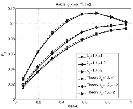
Figure 2: Comparison of the simulation and theoretical results for Method $3$.

From Figure 2, we observe that the probability of success as computed from the theory matches the simulations closely.

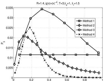
Figure 3: Probability of success for the four methods described in the previous section. The $x$-axis represents $\delta$ for Method $2$, $4\theta/\pi$ for Method $3$ and $\epsilon/6$ for Method $4$.

In Figure 3, the success probability is plotted for the four methods described in previous sections. We first observe that all the methods have an optimal value of the parameters $\delta$, $\theta$ and $\epsilon$ that achieve the maximum success probability. We also observe that Method $1$ has the worst performance. This is because of the high interference caused by all the relays (that have received a packet in the first hop) transmitting in the second hop. We observe that Method $3$ i.e., the sectorized selection method performs the best. Also observe that the RSS based selection has twice the $P_{s}$ as compared to Method $1$ in which every relay transmits. We also observe that the both the location-aware schemes outperform Method $1$ and Method $2$ for the particular values of $T=3,\lambda_{s}=1,\lambda_{r}=1.5$.

VI Conclusion

In this paper, we have have analyzed the success probability in a two hop system taking interference and spatial distribution of the nodes into account. We have provided an analytical solution for all the four methods using some approximations. This method of analysis can be easily extended to any position based relay selection. We have shown that uncoordinated selection of relays increases the success probability as compared to selecting a relay for each source-destination pair apriori.

Appendix

The probability that a destination located at $z$ can decode the packet transmitted by a source $\xi$ when the interference is caused by $\phi_{s}$ is

$$p_{\xi}(z) = \mathbb{P}\left(\xi\rightarrow z\mid\phi_{s}\right)$$ (6)

$$= \mathbb{P}\left(\text{SIR}(\xi,z\mid\phi_{s})>T\right)$$

$$= \mathbb{P}(h_{\xi z}>\frac{T}{g(\xi-z)}\sum_{x\in\phi_{s}}h_{xz}g(x-z))$$

$$\stackrel{{\scriptstyle(a)}}{{=}}\mathbb{E}\prod_{x\in\phi_{s}}\exp\left(-\frac{T}{g(\xi-z)}h_{xz}g(x-z)\right)$$

$$\stackrel{{\scriptstyle(b)}}{{=}}\exp(-\lambda_{s}\int_{\mathbb{R}^{2}}\beta(\xi-z,y)dy)$$

where

$$\beta(x,y)=\frac{1}{1+\frac{g(x)}{T}g(y)^{-1}}$$

$(a)$ follows from the exponential distribution of $h_{\xi z}$, and $(b)$ follows the probability generating functional (PGFL) of the PPP [1, 7]. Also observe that $p_{\xi}(z)$ depends only on $\|\xi-z\|$.

Direct transmission: So from (1) we have

$$P_{1} = \lim_{a\rightarrow\infty}\frac{1}{\lambda_{t}\pi a^{2}}\mathbb{E}\sum_{x\in\phi_{s}\cap B(o,a)}\mathbf{1}(x\rightarrow r(x)\mid\phi_{s})$$

$$\stackrel{{\scriptstyle(a)}}{{=}} \lim_{a\rightarrow\infty}\frac{1}{\pi a^{2}}\int_{B(o,a)}p_{x}(r(x))dx\ \stackrel{{\scriptstyle(b)}}{{=}}\ P_{o}(R),$$

where $(a)$ follows from the Campbell-Mecke theorem [7] and $(b)$ follows from he fact that $p_{\xi}(z)$ depends only on $\|\xi-z\|$.

First hop: A point process is completely characterized by its PGFL and so we will evaluate the PGFL of the relays which can connect to source $\xi\in\phi_{s}$, i.e., the cluster $\hat{\phi}_{r}(\xi)$. Let $0\leq v(x)\leq 1$. The PGFL of $\hat{\phi}_{r}(\xi)$ is given by

$$\mathcal{G}_{\xi}(v(x)) = \mathbb{E}\prod_{x\in\phi_{r}}1-(1-v(x))\mathbf{1}(\xi\rightarrow x\mid\phi_{s})$$

$$\stackrel{{\scriptstyle(a)}}{{=}} \mathbb{E}\exp\left(-\lambda_{r}\int_{\mathbb{R}^{2}}(1-v(x))\mathbf{1}(\xi\rightarrow x\mid\phi_{s})dx\right)$$

$$\stackrel{{\scriptstyle(b)}}{{\geq}} \exp\left(-\lambda_{r}\int_{\mathbb{R}^{2}}(1-v(x))p_{\xi}(x)dx\right),$$ (9)

where $(a)$ follows since $\phi_{r}$ is a PPP, and $(b)$ follows from Jensen’s inequality. From the PGFL we observe that the point process consisting of relays which connect to the origin is not a PPP. $(b)$ would have been an equality if $\mathbf{1}(\xi\rightarrow x\mid\phi_{s})$ are independent for different $x$ and the resulting process would be a PPP. But for the sake of analysis, we make the following assumptions and justify them by simulations.

1. We assume that the spatial distribution of $\hat{\phi}_{r}(\xi)$ is an inhomogeneous PPP with intensity $\lambda_{r}p_{\xi}(\xi)$. Since $T>1$, $\hat{\phi}_{r}(\xi_{1})\cap\hat{\phi}_{r}(\xi_{2})=\emptyset,\quad\forall\xi_{1},\xi_{2}\in\phi_{s}$.

2. We also assume $\hat{\phi}_{r}(\xi_{1})$ is independent of $\hat{\phi}_{r}(\xi_{2})$ for all $\xi_{1},\xi_{2}\in\phi_{s}$.

We will show the results obtained by this assumption are close to the actual by simulation. From Figure 2 we observe that the simulation results (for Method $3$) are very close to that predicted by theory making the above assumptions. This is intuitive since many terms in (Appendix) are independent and thus the bound in (9) is very tight.

A subset of relays $N_{\xi}\subseteq\hat{\phi}_{r}(\xi)$ for each $\xi\in\phi_{s}$ transmit in the second hop depending on the relay selection method. This is basically a thinning of the point process $\hat{\phi}_{r}(\xi)$. We will now derive the intensity of the point process $N_{\xi}$ for different methods. We will denote the spatial intensity of $N_{\xi}$ by $\Delta_{\xi}(z)$ and we have $\mathbb{E}[|N_{\xi}\cap A|]=\int_{A}\Delta_{\xi}(z)dz$ for any $A\subset\mathbb{R}^{2}$ .
Method $1$: Since $N_{\xi}=\hat{\phi}_{r}(\xi)$, we have $\Delta_{\xi}(z)=\lambda_{r}p_{\xi}(z)$.
Method $2$: From (11), we have

$$\Delta_{\xi}(z) = \lambda_{r}\mathbb{E}\left(\exp\left(-\delta\frac{\text{RSS}(z)}{1+T}\right)\mathbf{1}\left(\xi\rightarrow z\mid\phi_{s}\right)\right)$$

$$\stackrel{{\scriptstyle(a)}}{{=}} \lambda_{r}(1+T)\frac{\exp\left(-\lambda_{s}\int_{\mathbb{R}^{2}}\frac{(\delta g(\xi-z)+T)g(y)}{g(\xi-z)+(\delta g(\xi-z)+T)g(y)}dy\right)}{1+T+\delta g(\xi-z)},$$

where $(a)$ follows from a procedure similar to the evaluation of $p_{\xi}(z)$.
Method $3$: Given $\xi$ and $r(\xi)$, we have

$$\Delta_{\xi}(z)=\lambda_{r}p_{\xi}(z)\mathbf{1}(\angle z\xi r(\xi)<\theta).$$

Method $4$: Given $\xi$ and $r(\xi)$, we have

$$\Delta_{\xi}(z)=\lambda_{r}p_{\xi}(z)\exp\left(-\epsilon\|z-r(\xi)\|R^{-1}\right)$$

The average number of relays in a cluster $N_{\xi}$ that transmit in the second hop is $\int\Delta_{\xi}(z)dz$.

Second hop: The transmitting set in second hop is given by $\psi=\bigcup_{\xi\in\phi_{s}}N_{\xi}$. Since $T>1$, at most one transmitter belonging to $N_{\xi}$ can connect to $r(\xi)$. So the probability that no node from $N_{\xi}$ can connect to $r(\xi)$ denoted by $f(\xi)$ is given by

$$f(\xi) = 1-\sum_{z\in N_{\xi}}\mathbf{1}\left(z\rightarrow r(\xi)\mid\psi\right).$$

So $\tilde{P_{2}}$ (same as $P_{2}$ without the limit) is given by

$$\tilde{P_{2}} = \mathbb{E}\sum_{x\in\phi_{t}\cap B(o,a)}\sum_{z\in N_{\xi}}\mathbf{1}\left(z\rightarrow r(\xi)\mid\psi\right)$$

$$\stackrel{{\scriptstyle(a)}}{{=}} \lambda_{t}\int_{B(o,a)}\mathbb{E}\sum_{z\in N_{\xi}}\mathbf{1}\left(z\rightarrow r(\xi)\mid N_{\xi}\cup\psi\right)d\xi$$

$$\stackrel{{\scriptstyle(b)}}{{=}} \lambda_{t}\int_{B(o,a)}\int\mathbb{E}\left[\Delta_{\xi}(z)\mathbf{1}\left(z\rightarrow r(\xi)\mid N_{\xi}\cup\psi\right)\right]dzd\xi$$

where $(a)$ and $(b)$ follow from the Campbell-Mecke theorem and Slivnyak’s theorem. We included $\Delta_{\xi}(x)$ in the expectation operator because in Methods $3$ and $4$, $\Delta_{\xi}(z)$ depends on the random variable $r(\xi)$. We now show that the inner integral does not depend on $\xi$. We also have $\Delta_{\xi}(z)=\Delta_{o}(\xi-z)$ for Method $1$ and $2$. For Methods $3$ and $4$ we have $\Delta_{\xi}(z)\stackrel{{\scriptstyle d}}{{=}}\Delta_{o}(\xi-z)$ where the equality is in distribution. Using the substitution $z^{\prime}\leftarrow z-\xi$, the stationarity of $\psi$, and the above property of $\Delta_{\xi}(z)$ we have

$$P_{2}=\frac{1}{2\pi}\int_{0}^{2\pi}\int_{\mathbb{R}^{2}}\mathbb{E}\left[\Delta_{o}(z)\mathbf{1}\left(z\rightarrow R_{\nu}\mid\psi\cup N_{o}\right)\right]dzd\nu$$ (10)

where $R_{\nu}=(R\cos(\nu),R\sin(\nu))$. For Methods $1$ and $2$ by the isotropic nature of $N_{o}$ and $\psi$ we have

$$P_{2}=\int_{\mathbb{R}^{2}}\Delta_{o}(z)\mathbb{E}\mathbf{1}\left(z\rightarrow R\mid\psi\cup N_{o}\right)dz$$ (11)

Due to space constraints we will only describe how to derive $P_{2}$ for Method $3$. Method $4$ can be analyzed in a similar fashion. From (10) and the definition of $\Delta_{o}(z)$ for Method $3$, we have $P_{2}=$

$$\frac{\lambda_{r}}{2\pi}\int_{0}^{2\pi}\int p_{o}(z)\mathbb{E}\mathbf{1}(\angle zoR_{\nu}<\theta)\mathbf{1}\left(z\rightarrow R_{\nu}\mid\psi\cup N_{o}\right)dzd\nu$$

Since $\psi$ is isotropic we have

$$P_{2}=\frac{\lambda_{r}\theta}{\pi}\int p_{o}(z)\mathbb{E}\mathbf{1}\left(z\rightarrow R\mid\psi\cup\tilde{N}_{o}\right)dz.$$ (12)

Here $\tilde{N}_{o}$ is equal to $N_{o}\cap S(o,R,\theta)$ where $S(o,R,\theta)$ denotes a sector of angle $\theta$ on either side of the line joining the origin and $(R,0)$. With a slight abuse of notation we will denote $\tilde{N}_{o}$ also by $N_{o}$ and $N_{o}$ depends on the relay selection method. We now evaluate $\mathbb{E}\left[\mathbf{1}\left(z\rightarrow R\mid\psi^{\prime}\right)\right]$ where $\psi^{\prime}=\psi\cup N_{o}$.

$$\mathbb{E}\left[\mathbf{1}\left(z\rightarrow R\mid\psi^{\prime}\right)\right] = \mathbb{P}\left(h_{zR}g(z-R)>TI(\psi^{\prime},R)\right)$$ (13)

$$\stackrel{{\scriptstyle(a)}}{{=}} \mathbb{E}\exp\left(-\frac{TI(\psi^{\prime},R)}{g(z-R)}\right)$$

where $(a)$ follows from the exponential distribution of $h_{zR}$. Also (13) is the Laplace transform of the interference evaluated at $T/g(z-R)$. By our assumptions $\psi^{\prime}$ is a Poisson cluster process [4, 6] with an additional cluster at the origin. The Laplace transform of the interference in this case is given by $\mathbb{E}\exp\left(-s\sum_{y\in\psi^{\prime}}h_{yR}g(y-R)\right)$ which is equal to

$$\mathbb{E}\left[\prod_{y\in\psi^{\prime}}\exp\left(-sh_{yR}g(y-R)\right)\right]\stackrel{{\scriptstyle(a)}}{{=}}G_{\psi^{\prime}}\left(\frac{1}{1+sg(y-R)}\right)$$

where $G_{\psi}(.)$ is the PGFL of the process $\psi^{\prime}$ and $(a)$ follows by Laplace transform of the fading. So we have

$$\mathbb{E}\left[\mathbf{1}\left(z\rightarrow R\mid\psi^{\prime}\right)\right]$$

$$\stackrel{{\scriptstyle(a)}}{{=}} \mathbb{E}\left[\prod_{\xi\in\phi_{s}}\prod_{y\in N_{\xi}}\frac{1}{1+\frac{Tg(y-R)}{g(z-R)}}\right]\mathbb{E}\left[\prod_{y\in N_{o}}\frac{1}{1+\frac{Tg(y-R)}{g(z-R)}}\right]$$

$$\stackrel{{\scriptstyle(b)}}{{=}} \mathbb{E}\left[\prod_{\xi\in\phi_{s}}\exp\left(-\tilde{\beta}(z-R,\xi)\right)\right]\exp\left(-\tilde{\beta}(z-R,R)\right)$$

$$\stackrel{{\scriptstyle(c)}}{{=}} \exp\left(-\tilde{\beta}(z-R,R)-\lambda_{s}\int 1-\exp\left(-\tilde{\beta}(z-R,\xi)\right)d\xi\right),$$

where $(a)$ follows from assumption $2$, $(b)$ follows from a technique similar to the derivation of $p_{\xi}(z)$, $(c)$ follows from the PGFl of PPP, and where

$$\tilde{\beta}(z,\xi)=\int_{\mathbb{R}^{2}}\beta(z,y)\tilde{\Delta}_{o}(y+\xi)dy.$$

From the above equation, (12) and (11) we have,

$$P_{2}=\int_{\mathbb{R}^{2}}\tilde{\Delta}_{o}(z+R)$$

$$\cdot\exp\left(-\tilde{\beta}(z,R)-\lambda_{s}\int_{\mathbb{R}^{2}}1-\exp\left(-\tilde{\beta}(z,\xi)\right)d\xi\right)dz,$$

where $\tilde{\Delta}_{o}(z)=\Delta_{0}(z)$ for Method $1$ and $2$. For Method $3$, $\tilde{\Delta}_{o}(z)=\frac{\theta}{\pi}\lambda_{r}p_{\xi}(z)$. For Method $4$

$$\tilde{\Delta}_{o}(z)=\frac{\lambda_{r}}{2\pi}p_{\xi}(z)\int_{0}^{2\pi}\exp\left(-\epsilon\|z-R_{\nu}\|R^{-1}\right)d\nu.$$

References

• [1] Francois Baccelli, B.Β Blaszczyszyn, and P.Β Muhlethaler. An ALOHA protocol for multihop mobile wireless networks. IEEE Transactions on Information Theory, (2), Feb 2006.
• [2] A.Β Bletsas, A.Β Lippnian, and DPΒ Reed. A simple distributed method for relay selection in cooperative diversity wireless networks, based on reciprocity and channel measurements. In Vehicular Technology Conference, 2005. VTC 2005-Spring. 2005 IEEE 61st, volumeΒ 3.
• [3] S.Β Cui, A.M. Haimovich, O.Β Somekh, and H.V. Poor. Opportunistic Relaying in Wireless Networks. Arxiv preprint arXiv:0712.1169, 2007.
• [4] RadhaΒ Krishna Ganti and Martin Haenggi. Regularity, interference, and capacity of large ad hoc networks. In 40th Asilomar Conference on Signals, Systems, and Computers, Pacific Grove, CA, Oct 2006.
• [5] C.K. Lo, R.W. HeathΒ Jr, and S.Β Vishwanath. Opportunistic relay selection with limited feedback. Vehicular Technology Conference, 2007. VTC2007-Spring. IEEE 65th, pages 135–139, April 2007.
• [6] D.Β Stoyan. Inequalities and bounds for variances of point processes and fibre processes. Math. Operationsf. Statist., Ser.Statistics, 14:409–419, 1983.
• [7] Dietrich Stoyan, WilfridΒ S. Kendall, and Joseph Mecke. Stochastic Geometry and its Applications. Wiley series in probability and mathematical statistics. Wiley, New York, second edition, 1995.
• [8] M.Β Zorzi and R.R. Rao. Energy and latency performance of geographic random forwarding for ad hoc and sensor networks. Wireless Communications and Networking, 2003. WCNC 2003. 2003 IEEE, 3:1930–1935 vol.3, March 2003.