The XMM-Newton X-ray emission of the SNR N120 in the LMC

Abstract

We present new XMM-Newton observations of the supernova remnant N 120 in the LMC, and numerical simulations on the evolution of this supernova remnant which we compare with the X-ray observations. The supernova remnant N 120, together with several HII regions, forms a large nebular complex (also called N 120) whose shape resembles a semicircular ring. From the XMM-Newton data we generate images and spectra of this remnant in the energy band between 0.2 to 2.0 keV. The images show that the X-ray emission is brighter towards the east (i.e., towards the rim of the large nebular complex). The EPIC/MOS1 and MOS2 data reveal a thermal spectrum in soft X-rays. 2D axisymmetric numerical simulations with the Yguazú-a code were carried out assuming that the remnant is expanding into an inhomogeneous ISM with an exponential density gradient and showing that thermal conduction effects are negligible. Simulated X-ray emission maps were obtained from the numerical simulations in order to compare them with the observations. We find good agreement between the XMM-Newton data, previous optical kinematic data, and the numerical simulations; the simulations reproduce the observed X-ray luminosity and surface brightness distribution. We have also detected more extended diffuse X-ray emission probably due to the N 120 large HII complex or superbubble.

1 Introduction

X-ray emission from supernova remnants (SNRs), bubbles, and superbubbles provides an important means for the study of how the stars interact with the interstellar medium (ISM) and deliver part of their energy and matter to the galaxy that hosts them. It also gives important clues on the particular mechanisms involved such as supernova explosions and stellar winds. In the case of SNRs, the X-rays emitted allow us to diagnose their nature, to determine the energy released by the supernova explosion, to gain insight into the density distribution prior to the explosion, and to estimate the shock velocity and dynamical age, among other issues. It is also important to confront X-ray, optical, and radio observations with numerical simulations of SNR and bubble evolution, to discriminate the main characteristics of SNR evolution such as density gradients, thermal conductivity and magnetic fields, among others. This idea could be applied to more complex situations such as multiple SNR evolution, supernova explosions within wind-driven bubbles, or interactions between bubbles and SNRs, which we intend to explore in the future.

Accounting for all these motivations, we used XMM-Newton data of SNR N 120 in the Large Magellanic Cloud (LMC) to compare the X-ray luminosity and surface brightness distribution with results from axisymmetric numerical simulations obtained with the adaptive grid Yguazú-a code (see, for example, Velázquez et al. 2001). We selected this SNR because its kinematics (at optical wavelengths) has been already studied, having shown that the SNR is well differentiated from other neighboring nebulosities. An advantage of studying the X-rays from an object in the LMC is that the interstellar reddening towards this galaxy is small, thus making the LMC objects ideal to be studied at X-ray wavelengths. Furthermore, the distances to Galactic SNRs are not easy to determine while in the LMC all the objects are at the same (known) distance. Therefore, by selecting an SNR in the LMC (with a well known distance derived from several independent ways) we can be quite sure of its estimated linear diameter.

The supernova remnant N 120 (0519-697) was first identified as a SNR by Mathewson & Clarke (1973) through its non-thermal radio spectrum and its high [SII]/H$\alpha$ line-ratio. Its linear diameter is 30 pc for an LMC distance of 50 kpc (Feast 1999). Dickel & Milne (1998) obtained high spatial resolution radio-continuum maps at 1380 and 2378 MHz, showing a shell with a brightness enhancement towards the east, where the shell is well defined. They also confirm the non-thermal nature of the radio emission and obtain a spectral index $\alpha$ = –0.47. The X-ray emission from SNR N120 has been studied with Einstein data by Mathewson et al. (1983), who show that this SNR is one of the faintest X-ray sources among the known SNRs in the LMC (its derived X-ray luminosity is about 10³⁵ ergs^-1). SNR N 120 is located within the 9$\arcmin$ $\times$ 7$\arcmin$ (or 135 $\times$ 105 pc) arc-shaped nebular complex N 120 (Henize 1956) or DEM 134 (Davies et al. 1976), which consists of small wind-blown bubbles, HII regions, and the SNR N 120 along the rim at a common systemic velocity (Laval et al. 1992). Within this superbubble there has recently been detected OVI ($\lambda$1032 Å ) emission by FUSE (Sankrit & Dixon 2007) suggesting that shocked hot gas is present.

At optical wavelengths (H$\alpha$ and [SII]), SNR N 120 is seen as an ellipsoidal shell. The [SII] emission, as well as the highly receding H$\alpha$ emission show a shell whose eastern side is brighter than its western side (Georgelin et al. 1983, Rosado et al. 1993). The kinematics of SNR N 120 have been studied in detail by Rosado et al. (1993) by means of photometrically calibrated H$\alpha$ scanning Fabry-Perot observations. Rosado et al. (1993) also derive the following parameters for the SNR assuming that the optical emission is due to shocks induced by the primary blast wave in dense clumps: clump density, n_c = 8 cm^-3, intercloud density, n_b = 0.1 cm^-3, velocity of the shock induced in the clumps = 100 km s^-1, and shock velocity in the intercloud medium = 800 km s^-1. With these values, they computed a postshock temperature of 8.7 $\times$ 10⁶ K, an age of 7300 yr, and a released energy of 5 $\times$10⁵⁰ ergs.

In Section 2 we present the data and data reduction. Section 3 is dedicated to the presentation of the observational results and a discussion of their implications. In Section 4 we present the numerical code, the model and the results of our numerical simulations on the particular conditions found for SNR N 120, and in Section 5 we give the conclusions.

2 XMM-Newton Data and Data Reduction

SNR N 120 was observed with the XMM-Newton satellite (Jansen et al. 2001). The data were obtained during Revolution 0337 in October 2001 using the EPIC (European Photon Imaging Camera) which consists of two MOS (Metal Oxide Semi-conductor) CCD arrays (MOS1 & MOS2) (Turner et al. 2001), thus EPIC/MOS1 and EPIC/MOS2 cameras are used in this work (Obs ID 0089210701). EPIC cameras are CCD detectors with spectral resolution E/$\Delta$E $\sim$ 20-50 in the 0.1-10 keV band. The pointing coordinates were $\alpha$ (2000) = 05h18m42.0s, $\delta$ (2000) = –69$\arcdeg$39$\arcmin$30$\arcsec$. The two EPIC/MOS cameras were operated in the Full-Frame Mode, using the full 30$\arcmin$ field of view of XMM-Newton, covering the entire dimensions of SNR N 120 and including the nebular complex N 120, for a total exposure time of 62 ks.

For all observations, the Medium Filter was used. The Medium Filter is an aluminized optical blocking filter aimed at reducing the IR, visible and UV photons to which the EPIC/MOS cameras are also sensitive and whose detection would preclude the X-ray analysis. It is made of 1600 Å of poly-imide film with 800 Å of aluminium evaporated onto one side. This filter was used to prevent “optical loading” of the CCD, which can distort the X-ray spectra. The XMM-Newton pipeline products were processed using the XMM-Newton Science Analysis Software (SAS version 6.1.0). The data were taken in two intervals, hereafter referred to as “scheduled” and “unscheduled”. The difference between these two types of files arose because in the course of exposing the scheduled observations, there were interruptions due to high radiation levels; the exposures taken after the interruptions we call unscheduled.

The EPIC/MOS event files were screened to eliminate events due to charged particles or those associated with periods of high background; only events with CCD patterns 0-12 were selected. We discarded data with a high background (i.e., count rates $\geq$ 1.0 and 1.0 counts s^-1 for the EPIC/MOS1 and EPIC/MOS2 scheduled data, respectively, and 1.3 and 1.2 counts s^-1 for the EPIC/MOS1 and EPIC/MOS2 unscheduled data, in the background-dominated 10-12 keV energy range). The resulting exposure times are 13.5 and 13.6 ks for MOS1 and MOS2 scheduled, and 35.0 and 34.3 ks for MOS1 and MOS2 unscheduled data.

To obtain an image of the X-ray emission of SNR N 120, we merged the screened event files of all the EPIC observations. We extracted an EPIC image in the 0.2 - 2.0 keV band with a pixel size of 4$\arcsec$.35 and a PSF of 9$\arcsec$ estimated from point sources in the same field.

However, for the fitting of the X-ray spectrum of SNR N 120, we preferred not to merge the different data. This is because the exposure times were different and also because the task MERGE is not recommended for quantitative analysis. For the analysis of the X-ray spectrum the four individual data sets were simultaneously fitting using XSPEC. In this way, we extracted spectra from each of the four EPIC/MOS1 and MOS2 event files, scheduled and unscheduled, using a circular aperture of 80$\arcsec$ radius, large enough to include all the X-ray emission from the SNR. We determined the background level outside the source by extracting the spectrum in another circular aperture of similar radius to that of the source, well outside the SNR emission and without encompassing other X-ray sources. The background spectra were then scaled and subtracted from the source spectra. The four resulting spectra were analyzed jointly using the XSPEC spectral fitting package. We also extracted a spectrum from the merged event file, and analyzed this “merged” spectrum similarly, as a matter of comparison.

3 Results: X-ray Brightness Distribution, Luminosity and Spectrum of the SNR N 120

3.1 X-ray brightness distribution

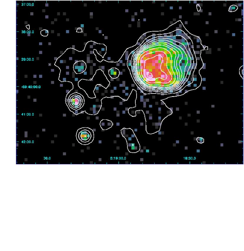
Figure 1: EPIC/MOS1$+$MOS2 color image of the X-ray emission of the SNR N 120 in the energy band from 0.2 to 2.0 keV. In white are overplotted the X-ray contours of the same X-ray image revealing the shape of the X-ray emission (from the 3rd contour). Contours have been drawn at levels of 1$\sigma$, 2$\sigma$, 3$\sigma$, 4$\sigma$, 5$\sigma$, 6$\sigma$, 7$\sigma$, 8$\sigma$, 10$\sigma$, 13$\sigma$, 16$\sigma$ and 18$\sigma$ above the background level.

Figure 1 shows the merged EPIC image in the 0.2–2.0 keV band (field-of-view =495$\arcsec$ $\times$354$\arcsec$), in false color, showing the X-ray emission of the SNR N 120, with contours of the same emission superposed. An image in the 2.0–5.0 keV band that we have produced (not shown) reveals no appreciable X-ray emission, and is very noisy.

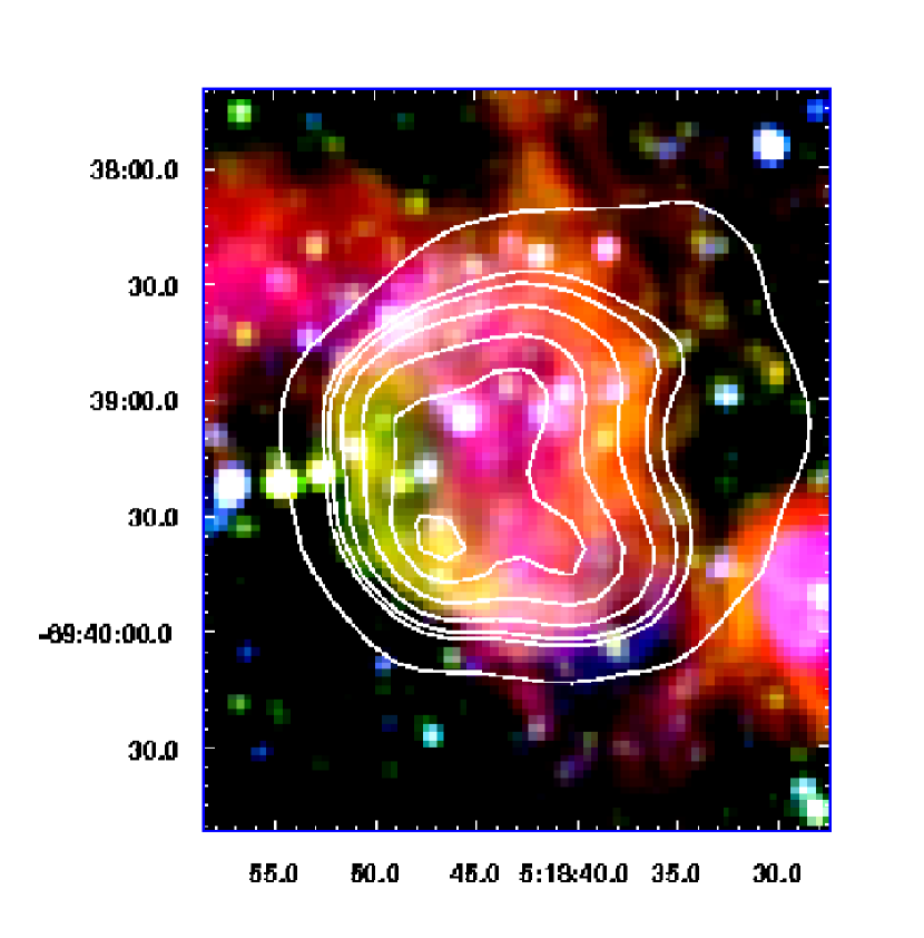
Figure 2: Three-color picture made up of Magellanic Clouds Emission-Line Survey (MCELS) images in H$\alpha$ (red), [SII] (green), and [OIII] (blue) of the SNR N 120. Superposed onto this picture are some of the X-ray contours (specially at levels of 3$\sigma$, 7$\sigma$, 8$\sigma$, 10$\sigma$, 13$\sigma$, 16$\sigma$ and 18$\sigma$) displayed in Figure 1.

As seen in Figure 1, the X-ray emission from the SNR (centered at $\alpha$ (2000) = 05h18m42.0s, $\delta$ (2000) = –69$\arcdeg$39$\arcmin$30$\arcsec$) shows an elliptical patch whose major axis is approximately oriented along the E-W direction, with a maximum elongation of 140$\arcsec$. The eastern side of this emission is much brighter than the western side, particularly at the eastern and southeastern boundaries. Figure 2 shows the three-color optical image (from the Magellanic Clouds Emission-Line Survey, MCELS) of the SNR 120 in the H$\alpha$ (red), [SII] (green), and [OIII] (blue) with some of the isocontours of X-ray emission depicted in Fig.1 overlayed for comparison. Inspecting this figure, we see that at optical wavelengths SNR N 120 appears as an elliptical shell of 108$\arcsec$ $\times$ 82$\arcsec$ (27 pc $\times$ 20 pc), whose major axis runs along the NE-SW direction. The bright eastern and southeastern X-ray rims correlate quite well with the limb-brightened optical [SII] emission at those locations (as well as with H$\alpha$ emission at high receding velocities; see Rosado et al.’s 1993 Figure 2). However, while the optical emission also appears ellipsoidal, its major axis is almost perpendicular to the major axis of the X-ray emission. The dimensions of the X-ray source (taken from the 3rd contour corresponding to a flux 3$\sigma$ above the background level) are 141$\arcsec$ $\times$ 127$\arcsec$ (equivalent to 34 pc and 31 pc at the LMC distance).

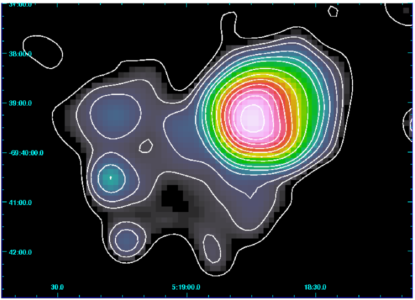
Figure 3: EPIC/MOS1$+$MOS2 Gaussian smoothed color image of the X-ray emission of the SNR N 120 in the energy band from 0.2 to 2.0 keV. In white are overplotted the X-ray contours of the same X-ray image. Contours have been drawn at levels of 4$\sigma$, 6$\sigma$, 8$\sigma$, 12$\sigma$, 16$\sigma$, 20$\sigma$, 30$\sigma$, 40$\sigma$, 50$\sigma$, 60$\sigma$, 70$\sigma$, 80$\sigma$, 90$\sigma$ and 100$\sigma$ above the background level.

A close inspection of Figure 1 suggested that the bright X-ray emission of SNR N 120 is embedded into faint, diffuse emission, well outside the boundaries of SNR 120. To gain insight regarding this diffuse and faint X-ray emission, we increased the signal to noise ratio by spatially smoothing the EPIC image shown in Figure 1 with a Gaussian function of 2.5 pixels width giving a scale of 11$\arcsec$ instead of the original scale of 4$\arcsec$.35 per pixel. Since the faint emission is diffuse, such a loss in angular resolution is not so important. The smoothed image is shown in Figure 3, also in false color and with contours of the emission superposed. From Figure 3 we see that, indeed, some diffuse X-ray emission is detected at faint levels (1st contour corresponding to a flux of 4 $\sigma$ above the background level) while SNR N 120 is the brightest source in the field.

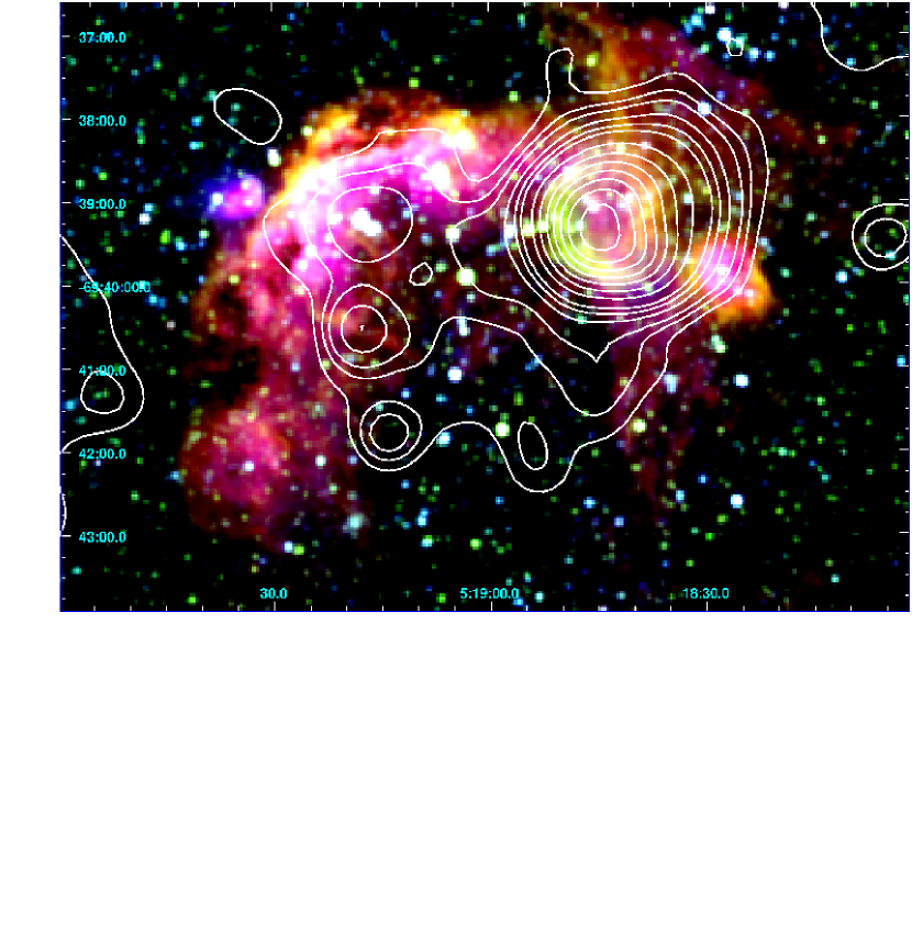
Figure 4: Three-color picture made up of MCELS images in H$\alpha$ (red), [SII] (green), and [OIII] (blue) of the N 120 nebular complex in the LMC. SNR N 120 is seen as the elongated bubble to the West. Superposed onto this picture are the X-ray contours of the 0.2-2.0 keV band displayed in Figure 3, in order to show the location of the diffuse X-ray emission. The optical images have $2\arcsec\times 2\arcsec$ pixels spatial resolution.

Figure 4 shows the surface brightness contours from Figure 3 (specially the 1st contour mapping the diffuse X-rays) superposed onto a larger field of view three-color image (from the MCELS) of the N 120 HII complex containing SNR N 120 in its NW boundary, in H$\alpha$ (red), [SII] (green), and [OIII] (blue). Note that the optical counterpart of SNR N 120 has the highest [SII]/H$\alpha$ ratio of all the nebulosities of the N 120 HII complex, as revealed from the colors in the MCELS image, and that the eastern rim of the shell has a higher [SII]/H$\alpha$ ratio than the western rim.

The faint, diffuse X-ray emission seems to correlate with some of the nebulae forming the N 120 complex (also called N 120 superbubble), all of them with thermal radio continuum emission (see Laval et al. 1992 for further details on their exact location and Dickel & Milne 1998 for further details about their radio spectral index). These nebulae are N 120B, N 120C1 and N 120C3 (to the East), part of N 120D (to the SW), part of the NW arc (N 140), and also covers part of the interior of the N 120 HII complex or superbubble. As mentioned in the Introduction, hot gas emitting in the UV has been detected from the N 120 superbubble (Sankrit & Dixon 2007) and, consequently, the diffuse, low intensity X-ray emission could come from the N 120 superbubble. The low intensity of the diffuse emission precludes obtaining insight into its origin from the available data. The diffuse X-ray emission could arise from hot gas escaping from the SNR N 120 or it could be associated with the N 120 superbubble, among other possibilities. However, the tenuous X-ray emission follows so well the overall morphology of the N 120 HII complex that we suggest that this faint emission could be associated with the N 120 superbubble and, therefore, not related to the SNR emission.

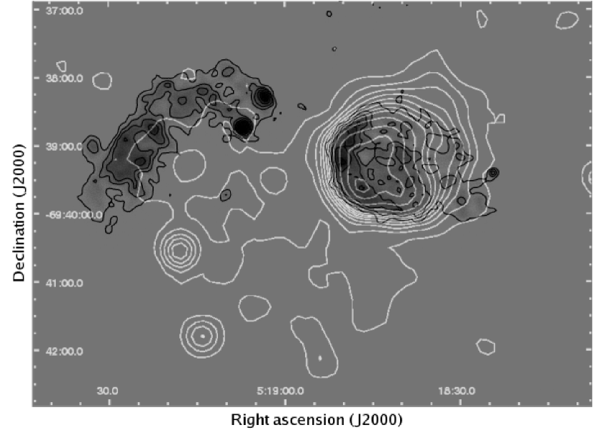
Figure 5: Radio contours of equal surface-brightness (in black) taken from Dickel & Milne (1998). Superposed on the radio contours are the X-ray contours of the 0.2-2.0 keV band (in white) displayed in Figure 1 (i.e., without any spatial smoothing ).

Figure 5 shows the contours of X-ray emission displayed in Figure 1 (i.e., at the original resolution 4$\arcsec$.35 per pixel) superposed onto the contours of the radio-continuum emission studied by Dickel & Milne (1998). The spatial resolution of the X-ray and radio-continuum contours is similar. Both emissions are seen elongated in the same direction and have, approximately the same extension. The brightness enhancement towards the eastern boundary of the SNR seen in X-rays coincides with a similar enhancement in the radio-continuum emission.

A previous X-ray image of SNR N 120 using ROSAT data was shown by Williams et al. (1999). Our image (Figures 1, 2 and 3) obtained with XMM-Newton data shows similar features: a bright ellipsoidal patch embedded in fainter emission. In both images, the brightest X-ray emission is located superposed onto the eastern rim of the optical emission. However the direct comparison with multiwavelength data (optical and radio) allowed us to have a more realistic interpretation of the X-ray data.

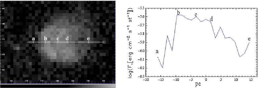
Figure 6: Left panel: EPIC/MOS X-ray emission map for SNR N 120 in the LMC. The white, horizontal line corresponds to the mean position of the ‘slit’ (the width of the aperture is $19\arcsec$ (5 pc) and the length is 174$\arcsec$ (42 pc)) along which the brightness profile was extracted. Right panel: X-ray surface brightness profile extracted along the horizontal line shown in the left panel. Some marks in both panels are given as reference of different locations.

To gain further insight into the soft X-ray emission of SNR N 120 we extracted a brightness distribution profile along the maximum elongation. Figure 6 (left) shows the mean aperture location (the width of the aperture is $19\arcsec$ (5 pc) and the length is 174$\arcsec$ (42 pc)) superposed onto the X-ray image and (right) the brightness distribution of the X-ray emission along this aperture. Several positions are indicated to facilitate the identification of features. From the brightness distribution profile, one can see that the maximum emission comes from the eastern region which coincides in location with the bright [SII] rim of the optical SNR. An irregular decrease in brightness follows towards the western boundary of the ellipsoidal patch. The irregularities in brightness found in the interior may be related to blobs of X-ray emission, which are less bright than the emission at the boundaries of the SNR.

3.2 X-ray spectrum and luminosity

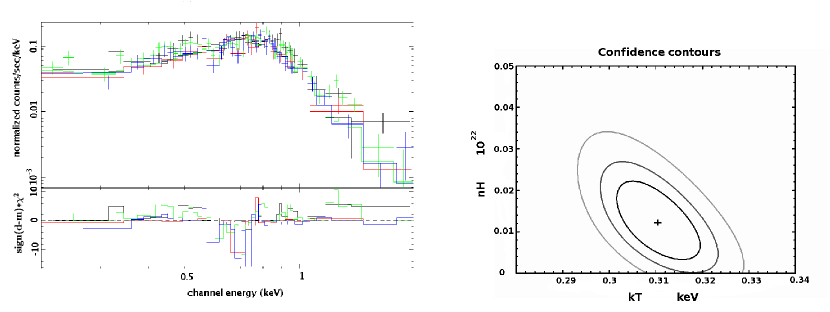
Figure 7: Left panel: X-ray spectrum of the scheduled MOS1 and MOS2 data (in black and red, respectively), and of unscheduled MOS1 and MOS2 data (in green and blue, respectively) analized jointly. Right panel:$\Delta\chi^{2}$ contours for an absorbed MEKAL: contours for 2D confidence levels of 68$\%$ (internal contour), 90$\%$ and 99$\%$ (external contour) are drawn. The cross indicates the model used in the fit of the left panel.

For spectral analysis, we used XSPEC, version 11.3.1 (Arnaud 1996). The spectra extracted from the EPIC/MOS1 and EPIC/MOS2 event files (as discussed in Section 2) are given in Figure 7. This figure shows that the spectrum is quite noisy for X-rays harder than about 2.0 keV. Therefore, we proceeded to model only the softer part of the spectrum having significant signal (up to 2.0 keV). In order to get the physical conditions of the X-ray emitting gas, we simultaneously modeled the MOS1 and MOS2 spectra by fitting different spectral models such as: 1) absorbed MEKAL optically-thin plasma emission models (Kaastra & Mewe 1993; Liedhal et al. 1995; Morrison & McCammon 1983), 2) absorbed PSHOCK models (Borkowski et al. 2001), and 3) absorbed non-equilibrium ionization, NEI, models (Borkowski et al. 2001). We froze the chemical abundances to the average value of the interstellar medium in the LMC (i.e., 0.3 times the solar abundances; Russel & Dopita 1992; Hughes et al. 1998), and we used reasonable values for the absorption column density, N_H, which should be in agreement with the measures of column densities in the LMC direction (Dickey & Lockman 1990), specifically, N_H $\simeq$ 1$\times$ 10²⁰cm^-2. In doing so, all considered models reproduce the observed spectra with reasonable $\chi^{2}$ statistics. Table 1 lists the parameters of the different fits to the X-ray spectra. It is interesting to note that PSHOCK and NEI models predict higher plasma temperatures. In view of the degeneracy of X-ray emission models with respect to the X-ray spectra, we selected the simplest emission model as representative of the X-ray spectrum of SNR N 120, that is, the one with the emission of a thermal optically-thin plasma in ionization equilibrium. It is possible that the plasma is not in ionization equilibrium, but the data we have do not allow us to discriminate this issue. In Figure 7 we reproduce (right panel) the plot of N_H versus kT for the confidence levels of the $\chi^{2}$ fit. Also displayed in Figure 7 is the best-fit model over-plotted on the EPIC spectra. In particular, this fit has an absorption column density of N_H = 1.21$\pm$0.66$\times$ 10²⁰cm^-2, in agreement with the measures of column densities in the LMC direction (Dickey & Lockman 1990), a plasma temperature of T = 6.0 $\times$ 10⁶ K (or kT = 0.31$\pm$0.06 keV ), and typical LMC abundances (see Table 2). The absorption-corrected X-ray luminosity in the 0.2–2.0 keV band is 1.2$\times$10³⁵ ergs $s^{-1}$ and flux 4.17$\times$ 10^-13 ergs cm² s^-1, confirming previous claims that SNR N 120 is one of the faintest SNRs detected in the LMC.

4 Numerical Simulations

4.1 The model

At radio frequencies, the SNR N 120 looks like an elongated shell with maximum elongation along the east-west direction. An increase of the radio continuum emission is observed to the east. This strong radio emission is correlated with strong [SII] emission (see Figures 2 and 5). As mentioned in Section 3, the X-ray brightness distribution also increases towards the east.

The brightness asymmetry could be produced by the collision of the SNR with high-density regions in the SNR environment, or by a density gradient of the ISM where the remnant is expanding. At high density sites, the emission in both radio and X-rays is enhanced. Around SNR N 120, there are several HII regions (N 120A, N 120B, N 120C and N 120D; see Laval et al. 1992) which, together with the SNR, comprise the N 120 superbubble. For these reasons, we have modeled the ISM around this remnant as a medium with increasing density to the east. Hnatyk & Petruk (1999) and Velázquez et al. (2004) studied the evolution of SNRs in this kind of ISM and found that radio continuum and X-ray morphologies, such as those observed in SNR N 120, can be reproduced by choosing an exponential density profile for the surrounding environment. In their study, Hnatyk & Petruk (1999) considered the importance of including projection effects, because the remnant could give the appearance of shell-like morphology at radio frequencies, while the morphology is a filled center in X-rays, i.e., the remnant belongs to the mixed-morphology or thermal-composite group, which could result from projection effects.

In the last 10 years, several theoretical works (Schneiter, de la Fuente & Velázquez 2006, Tilley & Balsara 2006, Velázquez et al. 2004, Cox et al. 1999, Shelton et al. 1999) analyzed the influence of thermal conduction on the morphology of SNRs, focusing on the case of the mixed-morphology SNR group. These works consider SNRs as expanding into dense environments (with numerical densities of the order of 10 cm^-3), producing a fast evolution of the remnant. The effects of thermal conduction on the SNR morphology in both radio and X-ray emission become important for more evolved SNRs, i.e., the remnants that have entered into the third phase of their evolution, the radiative phase. In this case, the remnant has a filled center in the X-ray band, while it is a shell-type in radio emission. Rosado et al. (1993) determine that SNR N 120 is in the second phase of evolution, also called the Sedov phase, and calculate an age for this remnant of 7300 yr. For these reasons, it seems that the effects of thermal conduction can be neglected for the SNR N 120 case. Nevertheless, we have also explored the effects of thermal conduction, as discussed below.

Based on these hypothesis, we have carried out numerical simulations modeling an SNR that evolves in a non-uniform ISM, with a density gradient in the form of an exponential law (this implies that there is a preferential direction). Because of this main characteristic of the ISM, we employ the 2D axisymmetric version of the Yguazú-a code (Raga et al. 2000 and also Raga et al. 2002), which has a binary adaptive grid. The symmetry axis is in the density gradient direction. The gas dynamic equations are integrated with a second-order accurate implementation of the flux vector splitting method of Van de Leer (1982) together with rate equations for the following atomic/ionic species: HI, HII, OI, OII, OIII, OIV, CII, CIII, CIV, HeI, HeII, HeIII, SII, SIII, NI, NII, and NIII, which determine the radiative cooling function.

4.2 Initial conditions

We have made three numerical simulations, employing a four-level binary adaptive grid in a 75$\times$37.5 pc (axial$\times$ radial) computational domain. The maximum resolution was 2.2$\times 10^{17}$ cm.

In the simulations, the SNR explodes into an ISM with an exponential density profile given by $n=n_{0}e^{-x/H}$, where $H$ is a characteristic length-scale, and n₀ is the density of the ISM at the position where the SN explosion occurs.

The SNR was located on the symmetry axis at the position $x_{SNR}=7.5\times 10^{19}$ cm or 25 pc. The SN explosion is simulated by imparting a sudden release of energy, $E_{0}$, to the medium, independent of the explosion mechanism and evolution of the pre-SN stage of the progenitor star. The released energy is put into an expanding 5 $M_{\odot}$ sphere of constant density and 1 pc radius which starts its interaction with the surrounding medium, simulating the SN explosion. Although this way of including the explosion does not give a good description of the early SNR evolution, for a SNR in the adiabatic phase or older (where $M_{ejected}<<M_{swept-up}$), the simulated explosion approaches in its effect an actual SN explosion. Incidentally, this approach has some basis if one considers that empirical mass-loss rates of solar metalicity stars with $M\geq 35M_{\odot}$ are thought to have pre-SN stages as hydrogen-free stars of about 5$M_{\odot}$ ( Woosley et al. 2002).

Based on Rosado et al. (1993) we chose an initial SN energy explosion, E₀, of $5\times 10^{50}$ erg, and an average ISM density (at the SNR position) of 0.1 cm^-3. The scale length, H, was set as 10 pc, 5 pc, and 3.67 pc for models 1, 2, and 3, respectively.

4.3 Simulated X-ray emission

Synthetic X-ray emission maps were generated from numerical simulations, in order to do a direct comparison with XMM-Newton observations. In all these simulations Ionization Equilibrium was assumed due to the following reasons. The observed spectra were fit employing different models, which consider Ionization Equilibrium (IEQ) and Non-equilibrium Ionization (NEI). We use the models MEKAL (IEQ) or pshock (NEI) and NEI (NEI). Simulated X-ray emission that considers NEI models, is based on 1D calculations (by analytical laws or 1D hydrodynamical simulations). These models fit well the observed spectra (see table 1) but give a partial hydrodynamical description of the SNR evolution. Since SNR N 120 exhibits a pronounced asymmetry, it implies that 1D models do not give a complete hydrodynamical description of this remnant. In view that our main goal is to reproduce the observed surface brightness distribution, and given that both IEQ and NEI models fit equally well the observed spectrum, for generating the simulated X-ray emission we considered IEQ models because they are simpler to implement and combine with our 2D numerical results. The main difference between NEI and IEQ models is that at low energies ($<2$ keV), IEQ models predict fluxes lower than the obtained by NEI (Hughes & Helfand 1985).

Thus, we used the CHIANTI database (Dere et al. 1997, Landi et al. 2006) for calculating the X-ray emission coefficient $j_{\nu}(n,T)$ in the energy range 0.15-2.0 keV. We consider an average abundance for the Large Magellanic Cloud of 0.3$Z_{\odot}$ and a column density $N_{HI}=1.2\times 10^{20}\ \rm{cm}^{-2}$, in agreement with the fit of the observed X-ray spectrum (see Section 3.2). We also consider the IEQ as given by the Mazzota et al. (1998) model. The $j_{\nu}(n,T)$ coefficients are calculated in the limit of low density resulting $j_{\nu}(n,T)\propto n^{2}$.

4.4 Theoretical results

In all models, the numerical simulations were carried out up to an integration time of 8000 yr (about the estimated age of SNR N 120 given by Rosado et al. 1993). At this time, the vertical diameter is of the order of 30 pc, in agreement with our X-ray observations. Also, we obtained from our numerical results a shock wave velocity of the order of $\mathrm{8}00\ km\ s^{-1}$, which coincides with the value given by the kinematical study of Rosado et al. (1993).

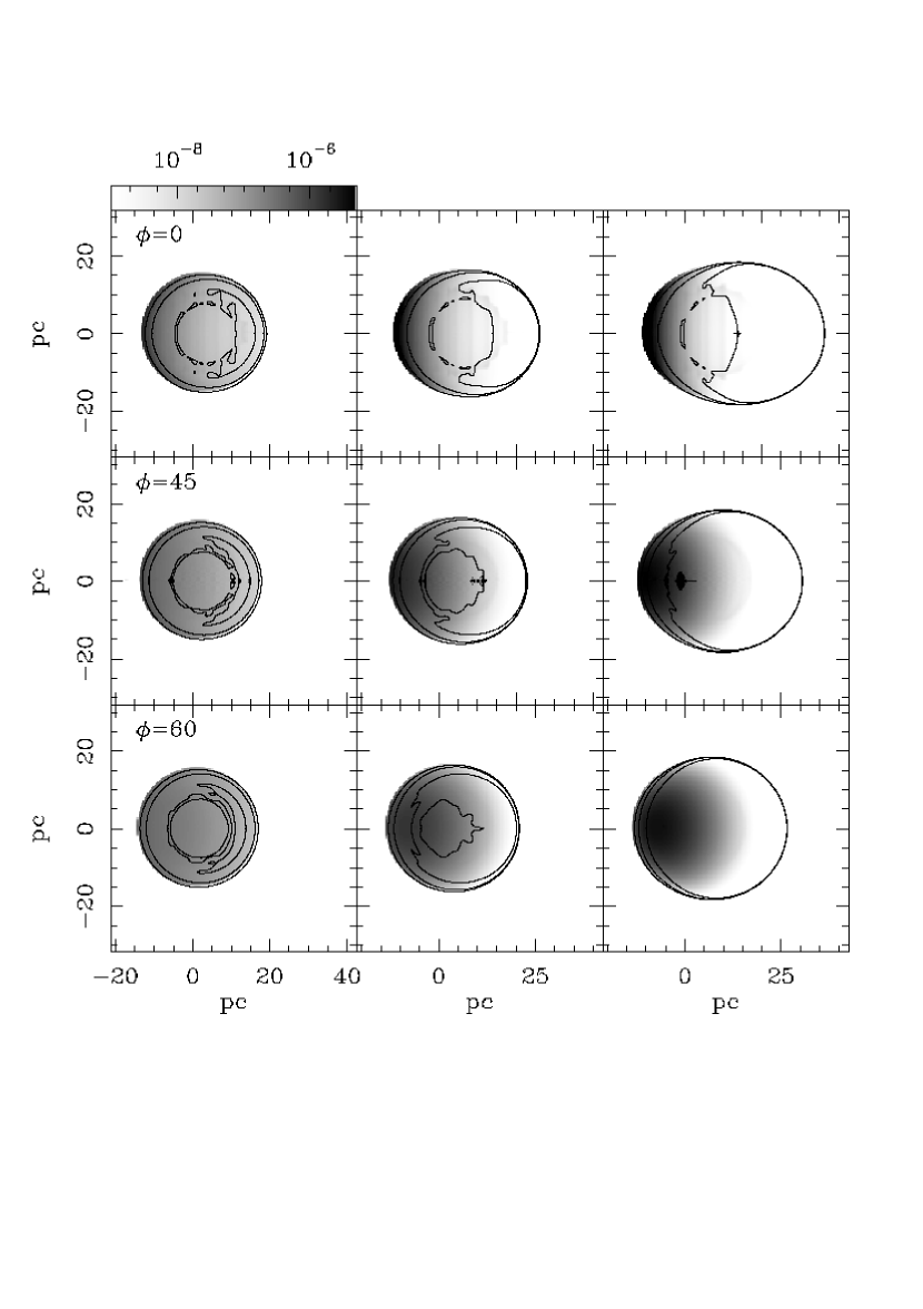
Figure 8: Simulated X-ray emission maps for models 1, 2 and 3 (left, central and right column panels, respectively). Different viewing angles between the symmetry axis and the plane of the sky, $\phi$ = 0$\arcdeg$, 45$\arcdeg$ and 60$\arcdeg$, are considered (top, central and bottom row panels, respectively). Overlaying the X-ray emission are plotted some contours of the temperature distribution, which trace the shock wave position. The linear grey-scale is given in units ergs cm^-2 s^-1 sr^-1; vertical and horizontal axis are given in pc.

Figure 8 compares the X-ray emission (in gray levels) obtained from models 1, 2 and 3 (left, central and right columns panels, respectively). In this figure, the projection effects were also explored generating maps where the angle, $\phi$, between the symmetry axis (the direction along which the ISM has a gradient in density) and the plane of the sky is 0$\arcdeg$, 45$\arcdeg$, and 60$\arcdeg$ (top, central and bottom row panels, respectively). Overlaying the X-ray emission, we show contours of the temperature distribution, integrated along the line of sight. Because the magnetic field is not included in our description, it was not possible to generate radio-continuum maps in order to obtain the actual size of the SNR shock wave. Therefore, it was necessary to look for other SNR shock wave tracers. One of them is the temperature integrated along the line of sight (Rodríguez-Martínez et al. 2006) since post-shock temperatures are higher ($T_{s}\propto v^{2}_{s}$, where $v_{s}$ is the shock-front velocity), reaching values $\sim$ 10⁷ – 10⁸ K. Thus, temperature contours describe shock front shapes.

Figure 8 shows that the SNR morphology is practically spherical for model 1, unlike models 2 and 3, where a pronounced elongation is seen in the horizontal direction. This effect is more noticeable for model 3 than for model 2. This morphology is in agreement with radio-continuum images of SNR N 120.

With respect to the spatial distribution of the X-ray emission, an increase in the X-ray surface brightness to the left is observed in all the maps. This increment is more important in the case of model 3. X-ray observations of this remnant also show an enhancement in the emission to the east (which corresponds to the left in our simulations). However, the X-ray maximum is located inside the SNR shell, close to the eastern border.

To better discriminate between our models and the observed X-ray enhancement towards the east, we have extracted X-ray surface-brightness profiles corresponding to the simulated maps displayed in Figure 8, i.e., for each model and for each viewing angle. The resulting surface-brightness profiles are displayed in Figure 9. The profiles correspond to horizontal cuts, passing through the center of the SNR shell. Profiles corresponding to model 3 (H = 3.67 pc) show a stronger enhancement of the X-ray emission to the left (corresponding to the east) than profiles obtained from model 1 (H = 10 pc).

Table 3 compares the X-ray luminosities obtained for all models, where ISM absorption associated with a column density of 1.2 $\times$ 10²⁰ cm^-2 has or has not been taken into account. The luminosity for model 3 is 8 $\times$ 10³⁴ ergs^-1, which is in better agreement with the observed value of 1.2 $\times$ 10³⁵ ergs^-1.

A comparison between Figure 9 (simulations) and Figure 6 (observations) suggests that models 2 and 3 (H = 5 pc and H = 3.67 pc, respectively), and viewing angles of 45$\arcdeg$ and 60$\arcdeg$, agree with the observed surface brightness profile in what concerns its actual dimensions (linear diameter about 30 pc) and slow decrease of X-ray surface brightness from east to west. On the other hand, model 3 fits best the observed X-ray luminosity of SNR N 120 (see Table 3).

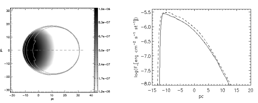
Figure 10: Left panel: simulated X-ray emission map for model 3 (H = 3.7 pc) and viewing angle $\phi$ = 45$\arcdeg$, smoothed at the same angular resolution than the observations. The dashed, horizontal line corresponds to the position along which the brightness profile was extracted. Right panel: X-ray surface-brightness profiles extracted along the horizontal of the left panel. The profile obtained for the case where thermal conduction is included in the calculation is displayed in dashed lines, while the case where thermal conduction is not included is represented by a solid line.

Figure 10 shows the simulated map corresponding to model 3 (H = 3.67 pc) viewed with an angle $\phi$=45$\arcdeg$, smoothed with the same angular resolution as the observations (left panel). From this map, a surface-brightness profile was extracted by tracing a cut along the maximum elongation direction (whose mean position is represented by the gray dashed line and its width is of 3 pixels in the vertical direction). This profile is depicted in the right panel of Figure 10 (solid line). A comparison between Figures 10 and 6 shows that our simulations reproduce the observed difference in surface brightness between the eastern and the western sides of the SNR, as well as the global decrease of the X-ray emission towards the west. However, the observed X-ray brightness profile shows secondary local maxima that are not reproduced by this model. This difference could arise because SNR N 120 is evolving in an ISM which has, in addition to the global density gradient in the east-west direction, several clumps or inhomogeneities. If one of these clumps was recently swept up by the remnant blast wave, its effect will be an increase of the X-ray emission projected onto the SNR interior.

To determine the importance of thermal conduction in the evolution of the SNR, another simulation, model 4, was made. This simulation employs the same parameters as model 3, with the inclusion of thermal conduction. The heat flux thermal conduction is included in the YGUAZÚ code by employing Spitzer’s (1962) classical expression $q=\kappa\nabla T$, where $\kappa=\beta T^{2.5}$ ( with $\beta\simeq 6\times 10^{-7}erg~{}s^{-1}K^{-1}cm^{-1}$), when the electron collisional mean free path $\lambda_{e}$ is less than the temperature scale height $L_{T}=T/{|\nabla T|}$. And, $q_{s}=-5\phi_{s}cP$ (Cowie & McKee 1977), where c is the isothermal sound speed, P is the gas pressure, and $\phi_{s}$ is a dimensionless parameter of the order of 1, when $\lambda_{e}>L_{T}$ and the heat flux is saturated. For details on the inclusion of classical and saturated thermal conduction in the YGUAZÚ-A code see Velázquez et al.(2004).

The luminosities found in the models with and without thermal conduction differ by only $10\%$. In Figure 10 we also present the surface brightness distribution along the maximum elongation predicted by model 4 (dashed lines). We have superposed the radial surface brightness profiles with and without considering thermal conduction. As seen in this figure, the effects of thermal conduction on the X-ray emission of SNR N 120 are negligible, as expected. Previous works have reported that the effects of thermal conduction are important for the case of more evolved SNRs, which have entered the third phase of evolution or radiative phase (Tilley et al. 2006). Therefore, the essential parameter in the evolution of the SNR is the density gradient of the interstellar medium.

We conclude that an exponential density gradient with a scale height of H = 3.67 pc for the ambient medium, where the SNR evolves, and view with an angle between 45$\arcdeg$ and 60$\arcdeg$, reproduce the main observed issues: total X-ray luminosity, dimensions and peculiar X-ray surface brightness profile. From the results of the last run (model 4) we also conclude that thermal conduction effects are negligible.

5 Summary

In this work we have presented XMM-Newton images and spectra of SNR N 120 in the LMC together with previous optical kinematic data, as well as numerical simulations that reproduce quite well the X-ray luminosity and surface brightness distribution of the SNR. Furthermore, the physical size and shock wave expansion velocity obtained from our numerical simulations are in agreement with the obtained ones by a previous kinematical study by Rosado et al. (1993).

We have found from XMM-Newton data that the X-ray emission of SNR N 120 consists of a conspicuous elliptical patch elongated along the E-W direction in the same way as the radio-continuum emission and with similar extension.

We have also found that the X-ray emission shows an asymmetry in brightness along the E-W direction and we have quantified this asymmetry by means of surface brightness profiles showing that the maximum X-ray surface brightness is emitted from the eastern boundary of the SNR. Secondary peaks in the brightness profile are also detected.

We have fitted reasonably well the X-ray spectrum of SNR N 120 with that of the thermal gas with LMC chemical abundances. Hence, we can conclude that the soft X-ray spectrum of this SNR is thermal.

We have also detected some faint and diffuse X-ray emission which shows some spatial correlation with the H$\alpha$ emission of the N 120 superbubble where SNR N 120 is at its boundaries. In view of the correlation, we suggest that the faint emission comes from the N 120 superbubble.

Working with the hypothesis that the asymmetry in X-ray emission is produced by the expansion of an SNR in an ISM with an exponential density profile, we have carried out several 2D axisymmetric numerical simulations of this model in order to check the validity of that hypothesis.

The density gradient could be due to the particular environment where the SNR N 120 is located: forming part of the boundary of the large nebular complex N 120.

The model that best fits the X-ray observations is the one with a density decreasing exponentially from the N 120 superbubble, with a scale length of 3.7 pc and with the assumption that the elongated X-ray emission is seen with its major axis inclined between 45$\arcdeg$ and 60$\arcdeg$ with respect to the plane of the sky. Secondary peaks in the X-ray surface brightness profile are not reproduced in our simulations and are probably due to the existence of ISM clumps recently shocked by the SNR blast wave.

We have also shown, by means of another numerical simulation (model 4), that thermal conduction effects are negligible for this SNR.

Figure 9: X-ray surface-brightness profiles for all panels shown in Figure 8. These profiles correspond to horizontal cuts, passing by the center of the SNR shell. The different viewing angles are marked in each panel. Solid lines: model 3, point hatched lines: model 2, and hatched lines: model 1.

Table 1: Parameters of Different Models Fitted to X-ray Spectra

Parameter	MEKAL	PSHOCK	NEI
NH	1.21 $\pm$0.66	2.0	2.0
(10${}^{20}cm^{-2}$)		(frozen)	(frozen)
kT	0.31 keV	0.49 keV	0.95 keV
Reduced $\chi^{2}$	1.60	1.35	1.93
$\tau$	–	0.0– 5.64 $\times 10^{11}$	2.32 $\times 10^{10}$
(cm-3s)

Table 2: MEKAL parameters corresponding to a simultaneous fit of the MOS1 and MOS2, scheduled and unscheduled data.

Parameters
NH $(10^{20}$ cm${}^{-2})$	$1.2\pm 0.66$
kT (keV)	$0.31\pm 0.06$
He	1.0
C	0.3
N	0.3
O	0.3
Ne	0.3
Na	0.3
Mg	0.3
Al	0.3
Si	0.3
S	0.3
Ar	0.3
Ca	0.3
Fe	0.3
Ni	0.3
$L_{x}$ $(10^{35}\ \rm{ergs\ s^{-1}})$	1.2
Flux $(10^{-13}\ \rm{ergs\ cm^{-2}s^{-1}})$	4.17

Table 3: X-ray luminosities from different models

	model 1	model 2	model 3	model 4 (with
				thermal conduction)
Length scale	10 pc	5 pc	3.67 pc	3.67 pc
$L_{x}(10^{35}ergs^{-1})$	0.16	0.44	0.81	0.92
$L_{x,abs}(10^{35}ergs^{-1})$	0.13	0.34	0.60	0.72

References

- Arnaud (1996) Arnaud, K. A. 1996, in ASP Conf. Proc. 101, Astronomical Data Analysis Software and Systems V, ed. G. Jacoby & J. Barnes (San Francisco: ASP), 17
- Borkowski et al. (2001) Borkowski, K.J., Lyerly, W.J. & Reynolds, S.P. 2001, ApJ, 548, 820
- (3) Cowie, L. L., & McKee, C. F. 1977, ApJ, 211, 135
- Cox et al. (1999) Cox, D.P., et al. 1999, ApJ, 524, 179
- Davies et al. (1976) Davies, R. D., Elliott, K.H., & Meaburn, J. 1976, MNRAS, 81, 89
- Dere et al. (1997) Dere, K. P., Landi, E., Mason, H. E., Monsignori Fossi, B. C., & Young, P. R. 1997, A&AS, 125, 149
- Dickel et al. (1998) Dickel, J.R., & Milne, D.K. 1998, AJ, 115, 1057
- Dickey et al. (1990) Dickey, J.M., & Lockman, F.J. 1990, ARA&A, 28, 215
- Feast (1999) Feast, M. 1999, PASP, 111, 775
- Georgelin et al. (1983) Georgelin, Y.M., Georgelin, Y.P., Laval, A., Monnet, G., & Rosado, M. 1983, A&AS, 54, 459
- Henize (1956) Henize, K.G. 1956, ApJS, 2, 315
- Hnatyk et al. (1999) Hnatyk, B., & Petruk, O. 1999, A&A, 344, 295
- Hughes & Helfand (1985) Hughes, J. P., & Helfand, D. J. 1985, ApJ, 291, 544
- Hughes et al. (1998) Hughes, J. P., Hayashi, I., & Koyama, K. 1998, ApJ, 505, 732
- Jansen et al. (2001) Jansen, F., Lumb, D., Altieri, B., et al. 2001, A&A, 365, L1
- Kaastra et al. (1993) Kaastra, J. S., & Mewe, R. 1993, Legacy, 3, 16
- Landi et al. (2006) Landi E., Del Zanna G., Young P. R., Dere K. P., Mason H. E., & Landini M. 2006, ApJS, 162, 261
- Laval et al. (1992) Laval, A., Rosado, M., Boulesteix, J., Georgelin, Y.P., Le Coarer,E., Marcelin, M., & Viale, A. 1992, A&A, 253, 213
- Liedahl et al (1995) Liedahl, D. A., Osterheld, A. L., & Goldstein, W. H. 1995, ApJ, 438, L115
- Mathewson et al. (1973) Mathewson, D. S., & Clarke, J. N. 1973, ApJ, 180, 725
- Mathewson et al. (1983) Mathewson, D. S., Ford, V. L., Dopita, M. A., Tuohy, I. R., Long, K. S., & Helfand, D. J. 1983, ApJS, 51, 345
- Mazzotta et al. (1998) Mazzotta, P., Mazzitelli,G., Colafrancesco, S.,& Vittorio, N. 1998. A&AS, 133, 403
- Morrison et al. (1983) Morrison, R., & McCammon, D. 1983, ApJ,270, 119
- Raga et al. (2000) Raga, A. C., Navarro-González, R., & Villagrán-Muniz M. 2000, RMxAA, 36, 67
- Raga et al. (2002) Raga, A. C., de Gouveia Dal Pino, E. M., Noriega-Crespo A., Mininni, P. D., & Velázquez, P. F. 2002, A&A, 392, 267
- Rodríguez-Martínez et al. (2006) Rodríguez-Martínez, M., et al., 2006, A&A, 448, 15
- Rosado et al. (1993) Rosado, M., Laval, A., Le Coarer, E., Boulesteix, J., Georgelin, Y. P., & Marcelin, M. 1993, A&A, 272,541
- Russel et al. (1992) Russel, S. C., & Dopita, M. A. 1992, ApJ, 384, 508
- Sankrit et al. (2007) Sankrit, R., & Dixon, W.V.D. 2007, PASP, 119, 284
- Shelton et al. (1999) Shelton, R.L. et al. 1999, ApJ, 524, 192
- Schneiter et al. (2006) Schneiter, E. M., de La Fuente, E., Velázquez, P. F.,2006, MNRAS, 371, 369
- Spitzer (1962) Spitzer, L., 1962, Physics of Fully Ionized Gases, Physics of Fully Ionized Gases. Interscience Publishers.
- Tilley et al. (2006) Tilley, D. A., Balsara, D. S., & Howk, J. C. 2006, MNRAS, 371, 1106
- Turner et al. (2001) Turner, M. J. L., Abbey, A., Arnaud, M., et al. 2001, A&A, 365, L27
- Van Leer (1982) Van Leer, B. 1982, ICASE Report 82-30
- Velázquez et al. (2001) Velázquez, P. F., Sobral, H., Raga, A. C., Villagrán-Muniz, M., & Navarro-González, R. 2001, RMxAA, 37, 87
- Velázquez et al. (2004) Velázquez, P. F., Martinell, J. J., Raga, A. C., & Giacani, E. B. 2004, ApJ, 601, 885
- Williams et al. (1999) Williams, R. M., Chu, Y.-H., Dickel, J. R., Petre, R., Smith, R. C., & Tavarez, M. 1999, ApJS, 123, 467
- Woosley et al. (2002) Woosley, S. E., Heger, A., & Weaver, T. A. 2002, RvMP, 74, 1015