Topologically massive gravity on AdS₂ spacetimes

Yun Soo Myung^1,a, Yong-Wan Kim ^1,b, and Young-Jai Park^2,c

¹Institute of Basic Science and School of Computer Aided Science,

Inje University, Gimhae 621-749, Korea

²Department of Physics, BK21 Program Division, Sogang University, Seoul 121-742, Korea

Abstract

We study the topologically massive gravity with a negative cosmological constant on AdS₂ spacetimes by making use of Kaluza-Klein dimensional reduction. For a constant dilaton, this two-dimensional model admits three AdS₂ vacuum solutions, which are related to AdS₃ and warped AdS₃ with an identification upon uplifting three dimensions. We carry out perturbation analysis around these backgrounds to find what is a physically propagating field. It turns out that the scalar perturbation $f$ of the Maxwell field $F_{\mu\nu}$ is nonpropagating in the absence of gravitational Chern-Simons terms, while it becomes a propagating mode with mass in the presence of gravitational Chern-Simons terms. This shows clearly that the number of propagating degrees of freedom is one for the topologically massive gravity. Moreover, at the points of $K=\pm l,l/3$, the mode $f$ becomes a massless scalar which implies that there exists still a propagating degree of freedom at the chiral points.

PACS numbers: 04.60.Kz, 04.70.Dy, 03.65.Sq, 03.65.-w.
Keywords: Topologically massive gravity; Perturbation; Dimensional reduction.

^aysmyung@inje.ac.kr
^bywkim65@gmail.com
^cyjpark@sogang.ac.kr

1 Introduction

The gravitational Chern-Simons terms in three dimensional (3D) Einstein gravity produce a physically propagating massive graviton [1]. This topologically massive gravity with a negative cosmological constant $\Lambda=-1/l^{2}$ (TMG_Λ) gives us the AdS₃ solution [2, 3]. For the positive Newton’s constant $G_{3}$, massive modes carry negative energy on the AdS₃. In this case, the AdS₃ is not a stable vacuum. The opposite case of $G_{3}<0$ may cure the problem, but it may induce a negative mass for the BTZ black hole.

There is a way of avoiding negative energy by choosing the chiral point of $K=l$ with the gravitational Chern-Simons coupling constant $K$. At this point, a massive graviton becomes a massless left-moving graviton, which carries no energy. It may be considered as pure gauge. However, the chiral point raises many questions on physical degrees of freedom (DOF) [4, 5, 6, 7, 8, 9, 10, 11].

Before we proceed, it is noted that the gravitational Chern-Simons terms are not invariant under coordinate transformations though they are conformally invariant [12, 13]. The variation of the gravitational Chern-Simons terms plays a role to find new solutions because it provides the Cotten tensor term in the equation of motion. It is known that the 3D Einstein gravity is locally trivial, while its quantum status remains unclear. All solutions to the 3D Einstein gravity are also solutions to the TMG_Λ. Furthermore, one needs to seek another method to investigate the TMG_Λ since it is likely a candidate for a nontrivial 3D gravity. One may introduce a conformal transformation to isolate the conformal DOF (dilaton mode). Then, the Kaluza-Klein ansatz is used to obtain an effective two-dimensional action (2DTMG_Λ), which will be a gauge and coordinate invariant action. Saboo and Sen [15] have used the 2DTMG_Λ to obtain the entropy of extremal BTZ black hole by using the entropy function formalism. This is possible because AdS₂ is a stable attractor solution of equations, which governs how near-horizon geometry changes as a degenerate horizon is being approached. On the other hand, for a constant dilaton, the authors in [16] have introduced the entropy function approach to find three AdS₂ vacuum solutions of the 2DTMG_Λ: AdS₂ with a positive charge, AdS₂ with a negative charge, and warped AdS₂ with a positive charge. Upon uplifting these solutions to three dimensions, they have obtained geometric solutions which are either AdS₃ or warped AdS₃ with an identification.

Hence it is very interesting to perform perturbation analysis of the 2DTMG_Λ, which shows what kind of field is really propagating on AdS₂ background. It is well known that there is no physical DOF for a graviton $h_{mn}$ propagating on AdS₃ in 3D Einstein gravity. Therefore, we must have zero DOF on AdS₂ after Kaluza-Klein reduction of 3D Einstein gravity: a two-dimensional graviton $h_{\mu\nu}=-h\bar{g}_{\mu\nu}$ (unphysical mode with $-1$ DOF), a gravivector $\delta F_{10}=-f$ (Maxwell mode with $0$ DOF), and a graviscalar $\varphi$ (dilaton mode with 1 DOF). However, we expect to have a massive mode in the 2DTMG_Λ because the gravitational Chern-Simons terms could generate a massive mode in the 3DTMG_Λ. It is supposed to be a mode like a gravivector.

In this work, we carry out perturbation analysis of the 2DTMG_Λ around three AdS₂ backgrounds. We show that a scalar perturbation $f$ of the Maxwell field $F_{\mu\nu}$ is trivial and nonpropagating in the absence of the Chern-Simons terms, while it becomes a massive propagating mode in the presence of the Chern-Simons terms. This shows clearly that the number of propagating DOF is one scalar for the 2DTMG_Λ. Moreover, at the chiral point of $K=\pm l,~{}l/3$, the mode $f$ becomes a massless scalar, which implies that there exists still a propagating DOF at this point.

2 Topologically massive gravity

We start with the action for topologically massive gravity with a negative cosmological constant given by [1]

$$I_{\rm TMG_{\Lambda}}=\frac{1}{16\pi G_{3}}\int d^{3}x\sqrt{-g}\Bigg{[}R_{3}-2\Lambda+\frac{K}{2}\varepsilon^{lmn}\Gamma^{p}_{~{}lq}\Big{(}\partial_{m}\Gamma^{q}_{~{}np}+\frac{2}{3}\Gamma^{q}_{~{}mr}\Gamma^{r}_{~{}np}\Big{)}\Bigg{]},$$ (1)

where $\varepsilon$ is the tensor defined by $\epsilon/\sqrt{-g}$ with $\epsilon^{012}=1$. We choose the positive Newton’s constant $G_{3}>0$. The Latin indices of $l,m,n,\cdots$ denote three dimensional tensors. The $K$-term is called the gravitational Chern-Simons terms. Here we choose “+” sign in the front of $K$ to avoid negative graviton energy [5]. It is the first higher derivative correction in three dimensions because it is the third-order derivative.

Varying this action leads to the Einstein equation

$$G_{mn}+KC_{mn}=0,$$ (2)

where the Einstein tensor including the cosmological constant is given by

$$G_{mn}=R_{3mn}-\frac{R_{3}}{2}g_{mn}-\frac{1}{l^{2}}g_{mn}$$ (3)

and the Cotton tensor is defined by

$$C_{mn}=\varepsilon_{m}~{}^{pq}\nabla_{p}\Big{(}R_{3qn}-\frac{1}{4}g_{qn}R_{3}\Big{)}.$$ (4)

We note that the Cotton tensor $C_{mn}$ vanishes for any solution to 3D Einstein gravity, so all solutions of general relativity are also solutions of the TMG_Λ. Hence, for $K=0$, the BTZ black hole [17] appears as a solution to Eq. (2)

$$ds^{2}_{BTZ}=-N^{2}(r)dt^{2}+\frac{dr^{2}}{N^{2}(r)}+r^{2}\Big{[}d\theta+N^{\theta}(r)dt\Big{]}^{2},$$ (5)

where the squared lapse $N^{2}(r)$ and the angular shift $N^{\theta}(r)$ take the forms

$$N^{2}(r)=-8G_{3}m+\frac{r^{2}}{l^{2}}+\frac{16G_{3}^{2}j^{2}}{r^{2}},~{}~{}N^{\theta}(r)=-\frac{4G_{3}j}{r^{2}}.$$ (6)

Here $m$ and $j$ are the mass and angular momentum of the BTZ black hole, respectively.

On the other hand, the warped black hole solution to the TMG_Λ was first considered in [18, 19], and a generalized warped black hole solution to the TMG without a cosmological constant was shown in  [20]. For $\nu^{2}=(\frac{l}{3K})^{2}>1$, the warped black hole solution, which is asymptotic to warped AdS₃, is allowed as [21, 22, 23]

$$ds^{2}_{wBH}=-\tilde{N}^{2}dt^{2}+\frac{l^{4}}{4\tilde{R}^{2}\tilde{N}^{2}}dr^{2}+l^{2}\tilde{R}^{2}\Big{(}d\theta+\tilde{N}^{\theta}dt\Big{)}^{2},$$ (7)

where

$$\tilde{R}^{2}(r)=\frac{r}{4}\left[3(\nu^{2}-1)r+(\nu^{2}+3)(r_{+}+r_{-})-4\nu\sqrt{r_{+}r_{-}(\nu^{2}+3)}\right],$$

$$\tilde{N}^{2}(r)=\frac{l^{2}(\nu^{2}+3)(r-r_{+})(r-r_{-})}{4\tilde{R}^{2}(r)},$$

$$\tilde{N}^{\theta}(r)=\frac{2\nu r-\sqrt{r_{+}r_{-}(\nu^{2}+3)}}{2\tilde{R}^{2}(r)}.$$ (8)

We note that for $\nu^{2}=1$, this metric reduces to the BTZ metric (5) in a rotating frame.

We would like to mention the AdS₃ solution (5) with $m=-1/8G_{3}$ and $j=0$. It is very important to find physical DOF of a massive mode propagating on the AdS₃ background when the Chern-Simons terms are present. There is no DOF in 3D Einstein gravity because there is $N_{c}=D(D-3)/2$ DOF in $D$ dimensional Einstein gravity . Hence it is evident that all components of $h_{mn}$ belong to gauge DOF.

On the other hand, we have $N^{m}_{c}=2$ DOF for a massive graviton in 3D Einstein gravity when including the Pauli-Fierz bilinear term of $I_{PF}=m^{2}_{PF}\int d^{3}x\sqrt{-\bar{g}}[h^{mn}h_{mn}-(h_{m}~{}^{m})^{2}]$ [24, 25] as a conventional mass term. However, it is worth to mention that the bilinear Chern-Simons term $K\int d^{3}x\sqrt{-\bar{g}}h^{mn}{\cal C}^{(1)}_{mn}$ [2] differs from the Pauli-Fierz term. Thus, the TMG_Λ may possess different physical DOF propagating on the AdS₃ spacetimes. Park has found $N^{m}_{c}=3$ [7], Carlip has obtained $N^{m}_{c}=1$ [10], while Grumiller et al. [8] have found $N^{m}_{c}=1$ in the chiral version of the theory [2]. Recently, it was shown that $N^{m}_{c}=1$, when using the full power of Dirac’s method for a constrained Hamiltonian system [26]. Moreover, at the chiral point of $K=l$, a massive graviton $\psi^{M}_{mn}$ turned out to be a left-moving graviton $\psi^{L}_{mn}$ (gauge degrees of freedom) [2, 27]. Grumiller and Johanson [5] have newly introduced a physical field $\psi^{new}_{mn}=\partial_{l/K}\psi^{M}_{mn}|_{K=l}$ as a logarithmic parter of $\psi^{L}_{mn}$ [5] based on the LCFT [28, 29, 30, 31, 32, 33]. However, it was reported that $\psi^{new}_{mn}$ might not be a physical field at the chiral point, since it satisfies fourth-order equation and thus it becomes a pair of dipole ghost fields with $\psi^{L}_{mn}$ [34].

Hence it would be better to use another method to show the existence of a massive mode in the TMG_Λ. Furthermore, to find a clear picture for a propagating mode at the chiral point, we study the effective two dimensional theory by making use of Kaluza-Klein reduction.

3 Dimensional reduction of TMG_Λ

We first make a conformal transformation and then perform Kaluza-Klein dimensional reduction by choosing the metric [12, 13]

$$ds^{2}=\phi^{2}\Big{[}g_{\mu\nu}(x)dx^{\mu}dx^{\nu}+\Big{(}d\theta+A_{\mu}(x)dx^{\mu}\Big{)}^{2}\Big{]}.$$ (9)

Here $\theta$ is a coordinate that parameterizes an $S^{1}$ with a period $2\pi l$. Hence, its isometry is factorized as ${\cal G}\times U(1)$. After the “$\theta$”-integration, the action (1) reduces to its effective two-dimensional action (2DTMG_Λ)

$$I_{\rm 2DTMG_{\Lambda}} = \frac{l}{8G_{3}}\int d^{2}x\sqrt{-g}\left(\phi R+\frac{2}{\phi}g^{\mu\nu}\nabla_{\mu}\phi\nabla_{\nu}\phi+\frac{2}{l^{2}}\phi^{3}-\frac{1}{4}\phi F_{\mu\nu}F^{\mu\nu}\right)$$ (10)

$$+ \frac{Kl}{32G_{3}}\int d^{2}x\left(R\epsilon^{\mu\nu}F_{\mu\nu}+\epsilon^{\mu\nu}F_{\mu\rho}F^{\rho\sigma}F_{\sigma\nu}\right).$$

Here $R$ is the 2D Ricci scalar with $R_{\mu\nu}-Rg_{\mu\nu}/2=0$ and $\phi$ is a dilaton as a graviscalar. Also, the Maxwell field $F_{\mu\nu}=2\partial_{[\mu}A_{\nu]}$ is defined by a gravivector $A_{\mu}$ and $\epsilon^{\mu\nu}$ is a tensor density. The Greek indices of $\mu,\nu,\rho,\cdots$ represent two dimensional tensors. Hereafter we choose $G_{3}=l/8$ for simplicity. It is noted that this action was used to derive the entropy of extremal BTZ black hole by applying the entropy function approach [15].

Introducing a dual scalar $F$ of the Maxwell field defined by [12, 13]

$$F=-\frac{1}{2\sqrt{-g}}\epsilon^{\mu\nu}F_{\mu\nu},$$ (11)

equations of motion for $\phi$ and $A_{\mu}$ are simplified, respectively, as

$$R+\frac{2}{\phi^{2}}(\nabla\phi)^{2}-\frac{4}{\phi}\nabla^{2}\phi+\frac{6}{l^{2}}\phi^{2}+\frac{1}{4}F^{2}=0,$$ (12)

$$\epsilon^{\mu\nu}\partial_{\nu}\left[\phi F-\frac{K}{2}(R+3F^{2})\right]=0.$$ (13)

The equation of motion for the metric $g_{\mu\nu}$ takes the form

$$g_{\mu\nu}\left(\nabla^{2}\phi-\frac{1}{l^{2}}\phi^{3}+\frac{1}{4}\phi F^{2}-\frac{1}{\phi}(\nabla\phi)^{2}\right)+\frac{2}{\phi}\nabla_{\mu}\phi\nabla_{\nu}\phi-\nabla_{\mu}\nabla_{\nu}\phi$$

$$-\frac{K}{2}\left[g_{\mu\nu}\left(\nabla^{2}F+F^{3}+\frac{1}{2}RF\right)-\nabla_{\mu}\nabla_{\nu}F\right]=0.$$ (14)

The trace part of Eq. (3)

$$\nabla^{2}\phi-\frac{2}{l^{2}}\phi^{3}+\frac{1}{2}\phi F^{2}-K\left(\frac{1}{2}RF+F^{3}+\frac{1}{2}\nabla^{2}F\right)=0$$ (15)

is relevant to our perturbation study. On the other hand, the traceless part is given by

$$g_{\mu\nu}\left(\frac{1}{2}\nabla^{2}\phi-\frac{1}{\phi}(\nabla\phi)^{2}\right)+\frac{2}{\phi}\nabla_{\mu}\phi\nabla_{\nu}\phi-\nabla_{\mu}\nabla_{\nu}\phi-\frac{K}{4}g_{\mu\nu}\nabla^{2}F+\frac{K}{2}\nabla_{\mu}\nabla_{\nu}F=0.$$ (16)

Now, we are in a position to find AdS₂ spacetimes as a vacuum solution to Eqs. (12), (13), and (15). In case of a constant dilaton, from Eqs. (12) and (15), we have the condition of a vacuum state

$$(3KF-2\phi)\left(\frac{\phi^{2}}{l^{2}}-\frac{1}{4}F^{2}\right)=0,$$ (17)

which provides three distinct relations between $\phi$ and $F$

$$\phi_{\pm}=\pm\frac{l}{2}F,$$ (18)

$$\phi_{w}=\frac{3K}{2}F.$$ (19)

We note that for $K=l/3$, $\phi_{w}=\phi_{+}$ which implies that it is a degenerate vacuum.

Assuming the line element preserving ${\cal G}=SL(2,R)$ isometry

$$ds^{2}_{AdS_{2}}=v\left(-r^{2}dt^{2}+\frac{dr^{2}}{r^{2}}\right),$$ (20)

we have the AdS₂ spacetimes, which satisfy

$$\bar{R}=-\frac{2}{v},~{}~{}~{}\bar{\phi}=u,~{}~{}~{}\bar{F}=e/v~{}(\bar{F}_{10}=e),$$ (21)

where $\bar{F}_{10}=\partial_{1}\bar{A}_{0}-\partial_{0}\bar{A}_{1}$ with $\bar{A}_{0}=er$ and $\bar{A}_{1}=0$. In order to find the whole solution of the AdS₂-type, we may use the entropy function formalism [16] because it provides an efficient way of finding AdS₂ solution as well as the entropy of corresponding extremal black hole. To this end, the entropy function is defined as

$${\cal E}(u,v,e,q)=2\pi\Big{[}qe-{\cal F}(u,v,e)\Big{]}$$ (22)

where ${\cal F}(u,v,e)$ is the Lagrangian density ${\cal L}_{\rm 2DTMG_{\Lambda}}$ evaluated when using Eq. (21),

$${\cal F}(u,v,e)=-2u+\frac{2u^{3}v}{l^{2}}+\frac{ue^{2}}{2v}+\frac{K}{2}\left(\frac{2e}{v}-\frac{e^{3}}{v^{2}}\right).$$ (23)

Upon the variation of ${\cal E}$ with respect to $u$, $v$, and $e$, equations of motion are obtained as

$$-2+\frac{6u^{2}v}{l^{2}}+\frac{e^{2}}{2v}=0,$$ (24)

$$\frac{2u^{3}}{l^{2}}-\frac{ue^{2}}{2v^{2}}-K\left(\frac{e}{v^{2}}-\frac{e^{3}}{v^{3}}\right)=0,$$ (25)

$$q-\frac{ue}{v}-\frac{K}{2}\left(\frac{2}{v}-\frac{3e^{2}}{v^{2}}\right)=0.$$ (26)

Equations (24) and (25) are those obtained by plugging Eq. (21) into Eqs. (12) and (15). This means that the entropy function formalism uses mainly the Einstein equation and dilaton equation in the near-horizon geometry AdS${}_{2}\times S^{1}$ of extremal BTZ black hole. A difference is that Eq. (13) is trivially satisfied with Eq. (21), while Eq. (26) is working for deriving the entropy.

Here we obtain three kinds of the AdS₂ solution:

(1) For $u=le/2v~{}(\phi_{+}=Fl/2)$, one has the AdS₂ solution with a positive charge $q$

$$u=\sqrt{\frac{ql^{2}}{2(l-K)}},~{}~{}~{}v=\frac{l-K}{2q},~{}~{}~{}e=\sqrt{\frac{l-K}{2q}}.$$ (27)

(2) For $u=-le/2v~{}(\phi_{-}=-Fl/2)$, the AdS₂ solution with a negative charge $q$ is found as

$$u=-\sqrt{\frac{-ql^{2}}{2(l+K)}},~{}~{}~{}v=-\frac{l+K}{2q},~{}~{}~{}e=-\sqrt{\frac{l+K}{-2q}}.$$ (28)

(3) For $u=3Ke/2v~{}(\phi_{w}=3FK/2)$, the warped AdS₂ solution with a positive charge $q$ is given by

$$u=\sqrt{\frac{9Kql^{2}}{l^{2}+27K^{2}}},~{}~{}~{}v=\frac{K}{q},~{}~{}~{}e=\sqrt{\frac{4Kl^{2}}{q(l^{2}+27K^{2})}}.$$ (29)

Then, corresponding entropies of the extremal black holes are given by

$$(1)~{}S_{+}=\frac{2\pi}{e}(l-K)\sim 2\pi\sqrt{\frac{ql}{6}\times\frac{12(l-K)}{l}},~{}~{}~{}l\geq K$$ (30)

$$(2)~{}S_{-}=\frac{2\pi}{e}(l+K)\sim 2\pi\sqrt{-\frac{ql}{6}\times\frac{12(l+K)}{l}},~{}~{}~{}l\geq-K$$ (31)

$$(3)~{}S_{w}=\frac{2\pi}{e}\frac{8Kl^{2}}{l^{2}+27K^{2}}\sim 2\pi\sqrt{\frac{ql}{6}\times\frac{96Kl}{l^{2}+27K^{2}}},~{}~{}~{}K>0.$$ (32)

The last relations ($\sim$) will be confirmed from the Cardy formula if $ql$ is justified as the eigenvalue of the $L_{0}$-operator of dual CFT₂. However, the AdS₂/CFT₁ correspondence is not still confirmed because we have two AdS₂ solutions [35, 36, 37, 38]: AdS₂ with a constant dilaton and near-horizon chiral CFT₂ (AdS₂/CFT₂ correspondence, in this work), and AdS₂ with a linear dilaton and asymptotic CFT₁ (AdS₂/CFT₁ correspondence). Finally, we mention that for $K=l/3$, $S_{+}=\frac{4\pi l}{3e}=S_{w}$ which shows a close connection between the two solutions (1) and (3).

4 Perturbation of 2DTMG_Λ around AdS₂

Now, let us consider the perturbation modes of the dilaton (graviscalar), graviton, and dual scalar around the AdS₂ background as

$$\phi = \bar{\phi}+\varphi,$$ (33)

$$g_{\mu\nu} = \bar{g}_{\mu\nu}+h_{\mu\nu},$$ (34)

$$F = \bar{F}(1+\delta F),$$ (35)

where the bar variables denote the AdS₂ background as $\bar{\phi}=u$, $\bar{g}_{\mu\nu}=v~{}{\rm diag}(-r^{2},r^{-2})$, and $\bar{F}=e/v$. This background corresponds to the near-horizon geometry of the extremal black holes, factorized as AdS${}_{2}\times S^{1}$. The Maxwell field has a scalar perturbation $f$ around the background: $F_{10}=\bar{F}_{10}+\delta F_{10}$, where $\delta F_{10}=\partial_{1}a_{0}-\partial_{0}a_{1}$ and $\delta F_{10}=-f$.

In this work, we choose the particular perturbation fields [39]

$$h_{\mu\nu}=-h\bar{g}_{\mu\nu},~{}~{}~{}\delta F=\left(h-\frac{f}{e}\right).$$ (36)

Taking the conformal gauge for $h_{\mu\nu}$ is quite reasonable for investigating the propagation of the graviton as an unphysical mode on the AdS₂ background. Even if one considers the off-diagonal components, these would be decoupled from $(\varphi,h,f)$. In addition, we note that the form of $\delta F$ is determined upon choosing the conformal gauge of $h_{\mu\nu}=-h\bar{g}_{\mu\nu}$. Hereafter, we wish to distinguish a dual scalar perturbation “$\delta F$” with a scalar perturbation “$f$”. The former is useful for diagonalizing process without sources, while the latter plays a key mode for our perturbation study with sources. In order to select $f$ appropriately, we need to use the source condition, which could decouple the unphysical mode $h$ from $f$ in $\delta F$.

However, we have to mention that there may be other types of perturbations, which lead to other linearized degrees of freedom.

4.1 $K=0$ perturbation

First, we study the $K=0$ case because this provides a reference case. Applying the linearizing process to (12), (13), and (15), the perturbed equations are given by

$$\bar{\nabla}^{2}h-\frac{2h}{v}-\frac{4}{u}\bar{\nabla}^{2}\varphi+\frac{12}{l^{2}}u\varphi+\frac{e^{2}}{v^{2}}\left(h-\frac{f}{e}\right)=0,$$ (37)

$$\epsilon^{\mu\nu}\partial_{\nu}\Bigg{[}\varphi+u\left(h-\frac{f}{e}\right)\Bigg{]}=0,$$ (38)

$$\bar{\nabla}^{2}\varphi-\frac{6}{l^{2}}u^{2}\varphi+\frac{ue^{2}}{v^{2}}\left(h-\frac{f}{e}\right)+\frac{e^{2}}{2v^{2}}\varphi=0.$$ (39)

Here we use $\delta R(h)=\delta R_{\mu\nu}(h)\bar{g}^{\mu\nu}-\bar{R}_{\mu\nu}h^{\mu\nu}=\bar{\nabla}^{\mu}\bar{\nabla}^{\nu}h_{\mu\nu}-\bar{\nabla}^{\sigma}\bar{\nabla}_{\sigma}h_{\mu}~{}^{\mu}-\bar{R}h_{\mu}~{}^{\mu}/2$ [2]. The perturbed equation (38) for the $F$-field leads to

$$\varphi+u\delta F=0,$$ (40)

which implies that the dual scalar $\delta F$ is a redundant mode (nothing but $\varphi$). For the AdS₂ solutions of $u=\pm\frac{le}{2v}$, the perturbed equation (39) together with Eq. (40) leads to equation for the dilaton

$$\left(\bar{\nabla}^{2}-\frac{2}{v}\right)\varphi=0,$$ (41)

which may indicate that the dilaton mode as a scalar is propagating on the AdS₂-background [40]. On the other hand, the perturbed equation (37) combined with (40) and (41) leads to the fourth-order equation for the graviton mode $h$

$$\left(\bar{\nabla}^{2}-\frac{2}{v}\right)^{2}h=0.$$ (42)

It is known from the counting of DOF that all of these modes belong to pure gauge because there is no physical DOF for the graviton $h_{mn}$ propagating on the AdS₃ background in the original 3D Einstein gravity. However, it seems that two modes of $\varphi$ and $\delta F$ are propagating on the AdS₂ background. Also, $h$ seems to be a propagating mode, even it satisfies the fourth-order equation. Therefore, it is necessary to show that all modes of $\varphi,h,f$ are nonpropagating on the AdS₂ background and then apply the same method to the linearized excitations in the $K\not=0$ TMG_Λ to determine which modes are propagating. Hence we need to employ a proper method to find physical DOF beyond the naive counting of DOF.

For this purpose, we compute the on-shell exchange amplitude (87) in Appendix A by plugging external sources $T,J_{\varphi},J_{f}$ into Eqs. (37), (39) and (40). Surprisingly, $J_{\varphi}$ completely disappears in this amplitude. It is important to note that when choosing the source condition of $T=\frac{e^{2}}{v^{2}}J_{f}$, the fourth-order unphysical pole disappears. Simultaneously, the second order pole disappears under this condition. Actually, imposing this proper source condition is equivalent to a decoupling process of the unphysical mode $h$ from the Maxwell mode $f$ in the dual scalar $\delta F$. In this case, the on-shell exchange amplitude (87) reduces to that of the Maxwell mode $f$ solely

$$\bar{A}^{K=0}=\frac{1}{2uv}\int d^{2}p[J^{2}_{f}].$$ (43)

As a result, the effective 2D gravity theory, which is matched with the original 3D Einstein gravity, has no physically propagating modes. Based on this analysis, we explore the effect of the gravitational Chern-Simons terms in the next section.

4.2 $K\neq 0$ perturbation

For $K\neq 0$, the perturbed equations of motion are complicated to have

$$\bar{\nabla}^{2}h-\frac{2}{v}h-\frac{4}{u}\bar{\nabla}^{2}\varphi+\frac{12}{l^{2}}u\varphi+\frac{e^{2}}{v^{2}}\delta F=0,$$ (44)

$$\epsilon^{\mu\nu}\partial_{\nu}\Bigg{[}\frac{e}{v}\Big{(}\varphi+u\delta F\Big{)}-\frac{K}{2}\Big{(}\bar{\nabla}^{2}h-\frac{2}{v}h+\frac{6e^{2}}{v^{2}}\delta F\Big{)}\Bigg{]}=0,$$ (45)

$$\bar{\nabla}^{2}\varphi-\frac{6}{l^{2}}u^{2}\varphi+\frac{e^{2}}{2v^{2}}\varphi+\frac{ue^{2}}{v^{2}}\delta F$$

$$-K\Bigg{(}\frac{e}{2v}\bar{\nabla}^{2}h-\frac{e}{v^{2}}h+\frac{e(3e^{2}-v)}{v^{3}}\delta F+\frac{e}{2v}\bar{\nabla}^{2}\delta F\Bigg{)}=0.$$ (46)

Eq. (45) implies

$$\frac{e}{v}\Big{(}\varphi+u\delta F\Big{)}-\frac{K}{2}\Big{(}\bar{\nabla}^{2}h-\frac{2}{v}h+\frac{6e^{2}}{v^{2}}\delta F\Big{)}=0.$$ (47)

Solving Eq. (47) for $\delta F$ and inserting it into Eq. (4.2), we obtain

$$\bar{\nabla}^{2}\varphi-\left(\frac{6u^{2}}{l^{2}}+\frac{e^{2}}{2v^{2}}\right)\varphi-\frac{Ke}{2v}\left(\bar{\nabla}^{2}-\frac{2}{v}\right)\delta F=0.$$ (48)

Since the second term can be further simplified as $(2/v)\varphi$, irrespective of the AdS₂ solutions (1), (2) and the warped AdS₂ solution (3), we find the same diagonalized equation as

$$\left(\bar{\nabla}^{2}-\frac{2}{v}\right)\left(\varphi-\frac{Ke}{2v}\delta F\right)=0$$ (49)

which may correspond to Eq. (41) for $K=0$. Moreover, solving Eq. (47) for $(\bar{\nabla}^{2}-\frac{2}{v})h$ and inserting it into Eq. (44), we obtain a coupled equation

$$\bar{\nabla}^{2}\varphi-\left(\frac{ue}{2vK}+\frac{3u^{2}}{l^{2}}\right)\varphi-\left(\frac{u^{2}e}{2vK}-\frac{5e^{2}u}{4v^{2}}\right)\delta F=0.$$ (50)

It reduces to

$$\left(\bar{\nabla}^{2}-\frac{2}{v}\right)\varphi-\left(\frac{ue}{2vK}-\frac{5}{4v}\right)\Big{(}\varphi+u\delta F\Big{)}=0$$ (51)

for the AdS₂ solutions (1) and (2), while it takes the form

$$\left(\bar{\nabla}^{2}-\frac{2}{v}\right)\varphi-\frac{1}{v}\left(\frac{l^{2}-27K^{2}}{l^{2}+27K^{2}}\right)\varphi+\frac{2l^{2}u}{v(l^{2}+27K^{2})}\delta F=0$$ (52)

for the warped AdS₂ solution (3).

Making use of Eq. (49), Eqs. (51) and (52) could be rewritten as two coupled equations for $\varphi$ and $\delta F$

$$\left(\bar{\nabla}^{2}-\frac{2}{v}\right)\delta F-\frac{2v}{Ke}\left(\frac{ue}{2vK}-\frac{5}{4v}\right)\Big{(}\varphi+u\delta F\Big{)}=0,$$ (53)

$$\left(\bar{\nabla}^{2}-\frac{2}{v}\right)\delta F-\frac{2}{Ke}\left(\frac{l^{2}-27K^{2}}{l^{2}+27K^{2}}\right)\varphi+\frac{2u}{Ke}\left(\frac{2l^{2}}{l^{2}+27K^{2}}\right)\delta F=0.$$ (54)

Acting $\left(\bar{\nabla}^{2}-\frac{2}{v}\right)$ on Eq. (53), and then eliminating $\varphi$ again by using Eq. (49), we arrive at the diagonalized equation for the dual scalar $\delta F$

$$\left(\bar{\nabla}^{2}-\frac{2}{v}\right)\left(\bar{\nabla}^{2}-m^{2}_{\pm}\right)\delta F=0,$$ (55)

for the AdS₂ solutions (1) and (2). Here, the mass $m^{2}_{\pm}$ is given by

$$m^{2}_{\pm}=\frac{2}{v}-\frac{1}{4v}\left(1\pm\frac{l}{K}\right)\left(5\mp\frac{l}{K}\right),$$ (56)

where the upper and lower signs denote the AdS₂ solutions (1) and (2), respectively.

For the warped AdS₂ solution (3), the diagonalized equation is found from Eq. (54) as

$$\left(\bar{\nabla}^{2}-\frac{2}{v}\right)\left(\bar{\nabla}^{2}-m^{2}_{w}\right)\delta F=0$$ (57)

whose mass $m^{2}_{w}$ takes the form

$$m^{2}_{w}=-\frac{3(l^{2}-9K^{2})}{v(l^{2}+27K^{2})}.$$ (58)

In deriving Eqs. (55) and (57), we assume that $(\bar{\nabla}^{2}-2/v)\delta F\not=0$. This is because if $(\bar{\nabla}^{2}-2/v)\delta F=0$, it may reduce to the $K=0$ case, as is shown in Eq. (41) for $\varphi=-u\delta F$. This implies that $m^{2}_{\pm,w}=2/v$ may be excluded in favor of a massive propagating mode. However, it is not true that solutions to the fourth-order equation $(\bar{\nabla}^{2}-2/v)^{2}\delta F=0$ are the same as those of the second-order equation $(\bar{\nabla}^{2}-2/v)\delta F=0$. This may be similar to the behavior of scalar fields at the Breitenlohner-Freedman bound in the AdS₄ spacetimes, where the disappearance of one branch solution is regarded as an illusion.

For $m^{2}_{\pm,w}\not=2/v$, Eqs. (55) and (57) may imply the second-order equations

$$\left(\bar{\nabla}^{2}-m^{2}_{\pm}\right)\delta F=0,~{}~{}\left(\bar{\nabla}^{2}-m^{2}_{w}\right)\delta F=0$$ (59)

which seem to be more attractive than the fourth-order equations.

However, we expect to obtain a single massive mode like $f$ which is propagating on the AdS₂ background because it turned out that $N^{m}_{c}=1$ for the $K\not=0$ case. Therefore, the second-order equations (59) are still far from our goal of finding $f$, even though the explicit masses are found. Inspired by the $K=0$ case, we wish to compute the on-shell exchange amplitude for the $K\not=0$ case, too. Actually, this was done in Appendix B by plugging the external sources $T,J_{\varphi},J_{f}$ into the linearized equations (44), (4.2), and (47). As is shown in Eq. (95), its form is very complicated, including poles of

$$\frac{1}{p^{2}+m^{2}},~{}~{}\frac{1}{(p^{2}+\frac{2}{v})(p^{2}+m^{2})},~{}~{}\frac{1}{(p^{2}+\frac{2}{v})^{2}(p^{2}+m^{2})}$$ (60)

with the mass $m^{2}=m^{2}_{\pm,w}$. We note that Eqs. (55) and (57) correspond to the second pole in the above. However, it is very difficult to isolate a physical amplitude including $\frac{1}{p^{2}+m^{2}}$ only. Hopefully, inspired by the $K=0$ case, we may choose the same source condition $T=\frac{e^{2}}{v^{2}}J_{f}$ to have a physical amplitude. Requiring this condition, the Fourier-transformed on-shell amplitude is reduced to a very simple expression

$$\bar{A}^{K}_{\pm,w}=\frac{u}{8}\int d^{2}p\frac{1}{{p}^{2}+m_{\pm,w}^{2}}\left(\frac{2e}{Kv}J_{f}-J_{\varphi}\right)^{2},$$ (61)

which contains $f$ and $\varphi$-amplitudes only. This confirms that the source condition decouples the unphysical mode $h$ from $\bar{A}^{K}_{\pm,w}$ effectively, remaining the $J_{f}$ and $J_{\varphi}$-amplitudes. We can check easily that this expression approaches the $K=0$ amplitude in the limit of $K\rightarrow 0$: Explicitly, the action (87) is exactly recovered from (61).

It seems appropriate to comment on why the dilaton mode appears in the $K\not=0$ amplitude, in comparison with the absence of $J_{\varphi}$ in the $K=0$ amplitude. The dilaton is the conformal mode, which is surely the pure gauge in view of the 3D Einstein gravity. As was shown in footnote 3, we have a relation of $\phi\sim f$ under the source condition. Hence, we may regard the dilation as a redundant mode, even it takes the same massive pole as the mode $f$ does.

Now we are in a position to analyze what these amplitudes are implied.

(1) For the AdS₂ solution with a positive charge, the allowable range is defined to be $l\geq K$. This is required for a positive entropy. Figure 1 shows the graph for mass $m^{2}_{+}$ and entropy $S_{+}$ versus $K$. The one-shell exchange amplitude is given by

$$\bar{A}^{K}_{+}=\frac{u}{8}\int d^{2}p\frac{1}{{p}^{2}+m_{+}^{2}}\left(\frac{l}{uvK}J_{f}-J_{\varphi}\right)^{2}.$$ (62)

At the chiral point of $K=l$, we have zero mass $m^{2}_{+}=0$. Then, its amplitude leads to

$$\bar{A}^{K=l}_{+}=\frac{u}{8}\int d^{2}p\frac{1}{{p}^{2}}\left(\frac{J_{f}}{uv}-J_{\varphi}\right)^{2},$$ (63)

which implies that the mode $f$ is massless. Actually, this interpretation is consistent with $N_{c}=1$  [8, 10, 26], which states that there is still a physical DOF at the chiral point. For $K=l/3$, we have zero mass $m^{2}_{+}=0$ but its amplitude takes a slightly different form

$$\bar{A}^{K=l/3}_{+}=\frac{u}{8}\int d^{2}p\frac{1}{{p}^{2}}\left(\frac{3J_{f}}{uv}-J_{\varphi}\right)^{2}.$$ (64)

Comparing it with Eq. (63), this case could be also considered as the massless propagation at another chiral point.

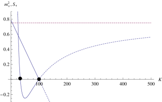
Figure 1: Mass $m^{2}_{+}$ and entropy $S_{+}$ for the AdS₂ solution with a positive charge for $l=100$, $v=1$: The curve is for the mass and the straight line for the entropy which is scaled to compare with the mass. The right-hand point ($\bullet$) is the chiral point ($K=l$), while the left-hand point ($\bullet$) is another chiral point $K=l/3$. Since the AdS₂ solution with a positive charge is valid for $l\geq K$, the permitted region is $0\leq K\leq 100$ but not $K>l$.

Figure 2: Mass $m^{2}_{-}$ and entropy $S_{-}$ for the AdS₂ solution with a negative charge for $l=100$, $v=1$: The curve is for the mass and the straight line for the entropy. The right-hand point ($\bullet$) is another chiral point ($K=-l/3$), while the left-hand point ($\bullet$) is the chiral point ($K=-l$). Since the AdS₂ solution with a negative charge is valid for $l\geq-K$, the permitted region is $-100\leq K\leq 0$ but not $K<-l$ .

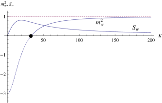
Figure 3: Mass $m^{2}_{w}$ and entropy $S_{w}$ for the warped AdS₂ solution with $K\geq 0$. The point ($\bullet$) denotes a chiral point ($K=l/3,\nu=1$). We have two limits: $m^{2}_{w}\to-1/3$ as $K\to 0$ and $m^{2}_{w}\to 1$ as $K\to\infty$.

(2) For the AdS₂ solution with a negative charge, the permitted range is defined to be $l\geq-K$. This is required for a positive entropy. Figure 2 shows the graph for mass $m^{2}_{-}$ and entropy $S_{-}$ versus $K$. The one-shell exchange amplitude is given by

$$\bar{A}^{K}_{-}=\frac{u}{8}\int d^{2}p\frac{1}{{p}^{2}+m_{-}^{2}}\left(\frac{l}{uvK}J_{f}+J_{\varphi}\right)^{2}.$$ (65)

At the chiral point of $K=-l$, we have zero mass $m^{2}_{-}=0$. Then, its amplitude leads to

$$\bar{A}^{K=-l}_{-}=\frac{u}{8}\int d^{2}p\frac{1}{{p}^{2}}\left(\frac{J_{f}}{uv}+J_{\varphi}\right)^{2},$$ (66)

which implies that the mode $f$ is massless. This interpretation is consistent with $N_{c}=1$  [8, 10, 26], which states that there is still a physical DOF at the chiral point. For $K=-l/3$, we have zero mass $m^{2}_{-}=0$ but its amplitude takes a different form

$$\bar{A}^{K=-l/3}_{-}=\frac{u}{8}\int d^{2}p\frac{1}{{p}^{2}}\left(\frac{3J_{f}}{uv}+J_{\varphi}\right)^{2}.$$ (67)

Comparing it with Eq. (66), this case may be considered as the massless propagation at another chiral point.

(3) For the warped AdS₂ solution, there is no restriction on $K$ because the positive entropy is guaranteed for $K\geq 0$. The one-shell exchange amplitude is given by

$$\bar{A}^{K}_{w}=\frac{u}{8}\int d^{2}p\frac{1}{{p}^{2}+m_{w}^{2}}\left(\frac{3}{uv}\frac{4l^{2}}{l^{2}+27K^{2}}J_{f}-J_{\varphi}\right)^{2}.$$ (68)

As is shown in Fig. 3, we have zero mass $m^{2}_{w}=0$ for $K=l/3$. Its amplitude takes the form

$$\bar{A}^{K=l/3}_{w}=\frac{u}{8}\int d^{2}p\frac{1}{{p}^{2}}\left(\frac{3J_{f}}{uv}-J_{\varphi}\right)^{2}=\bar{A}^{K=l/3}_{+}.$$ (69)

We prove a close connection that for $K=\frac{l}{3}$, the warped AdS₂ amplitude $\bar{A}^{K}_{w}$ is equal to $\bar{A}^{K}_{+}$ of the AdS₂ solution with a positive charge. For $K<l/3(\nu<1)$, $f$ has a negative mass, while for $K>l/3(\nu>1)$, $f$ has a positive mass. It is consistent with the propagation of the massive graviton on the warped AdS₂ background in the TMG_Λ.

5 Discussions

We have first discussed the perturbation of the effective 2D Einstein gravity around the AdS₂ background. For the $K=0$ case, it seems that a dual scalar perturbation $\delta F=(h-f/e)$ of the Maxwell field is equal to the dilaton mode $\varphi$, and they satisfy the second-order equation (41). This may imply that the modes $\delta F$ and $\varphi$ are propagating on the AdS₂ background. We note that it would be better to use the dual scalar $\delta F$ in the perturbation calculation, while the Maxwell scalar $f$ is a candidate for the physical mode. Consequently, we have successfully shown that there is no propagating modes on the AdS₂ background by calculating the on-shell exchange amplitude with the source condition of $T=\frac{e^{2}}{v^{2}}J_{f}$, which arises from the diffeomorphism (gauge symmetry). In this case, the dilaton mode $\varphi$ disappears in the amplitude. This reflects that the effective 2D gravity, which is matched with the 3D Einstein gravity, has no physically propagating degrees of freedom on the AdS₂ background because all modes of $h,\varphi,f$ are pure gauge.

For the $K\not=0$ case, it seems that $\delta F$ becomes the massive mode, which is propagating on the AdS₂ background. Considering the relation (49), it is conjectured that the dilaton mode $\varphi$ is propagating on the AdS₂ background, too. However, this is not true because the unphysical graviton mode $h$ is still involved in $\delta F$. In order to obtain physically propagating modes, we have computed the on-shell exchange amplitude. It takes a complicated form so that we could not isolate the physical amplitude from the full amplitude. Fortunately, inspired by the $K=0$ case, a proper choice of the source condition simplifies the on-shell amplitude significantly, leaving the massive pole for any AdS₂ background. As a result, we have clearly shown that the Maxwell scalar $f$ is a truly massive mode propagating on the AdS₂ background.

Appendix: On-shell exchange amplitudes with external sources

A. $K=0$ case

In order to find physically propagating modes of the effective 2D gravity on the AdS₂ background, we start with the action (10) with $K=0$. Its bilinear form is coupled with external sources as

$$A^{K=0}=\int d^{2}x\left[\delta_{2}{\cal L}_{\rm 2Dgravity}(h,\varphi,f)+h_{\mu\nu}T^{\mu\nu}+\varphi J_{\varphi}+\frac{e}{v^{2}}fJ_{f}\right].$$ (70)

Here, $\delta_{2}{\cal L}_{\rm 2Dgravity}$ is the bilinear action of effective 2D gravity around the AdS₂ background, and the external sources are given by $T^{\mu\nu}(x),J_{\varphi}(x),J_{f}(x)$ for the graviton, dilaton, and scalar of the Maxwell field, respectively. In order to make the connection with Sec. 4.1, the above action could be rewritten in terms of the dual scalar perturbation $\delta F$

$$A^{K=0}=\int d^{2}x\left[\delta_{2}{\cal L}_{\rm 2Dgravity}(h,\varphi,\delta F)+h(-T+\frac{e^{2}}{v^{2}}J_{f})+\varphi J_{\varphi}-\frac{e^{2}}{v^{2}}\delta FJ_{f}\right]$$ (71)

with the trace $T=\bar{g}^{\mu\nu}T_{\mu\nu}$. In order to investigate what physical excitations there are, we have to derive the linearized equations. At this stage, let us introduce the diffeomorphism generated by the coordinate transformation [12]

$$x^{\mu}\to\tilde{x}^{\mu}=x^{\mu}-\epsilon^{\mu}(t,r).$$ (72)

Then, the dilaton, gauge field, and metric transform as follows

$$\delta\tilde{\varphi} \to \delta\varphi+\epsilon^{\mu}\partial_{\mu}\bar{\phi},$$

$$\delta\tilde{a}_{\mu} \to \delta a_{\mu}+\epsilon^{\nu}\partial_{\nu}\bar{A}_{\mu}+\bar{A}_{\nu}\partial_{\mu}\epsilon^{\nu}+\partial_{\mu}\Lambda,$$ (73)

$$\delta\tilde{h}_{\mu\nu} \to \delta h_{\mu\nu}+\epsilon^{\rho}\partial_{\rho}\bar{g}_{\mu\nu}+\bar{g}_{\mu\sigma}\partial_{\nu}\epsilon^{\sigma}+\bar{g}_{\nu\sigma}\partial_{\mu}\epsilon^{\sigma},$$

where $a_{\mu}$ also undergoes an Abelian gauge transformation with gauge function $\Lambda(t,r)$. For the AdS₂ background in Eqs. (20) and (21), the relevant transformations lead to

$$\delta\tilde{\varphi} \to \delta\varphi,$$

$$\delta\tilde{a}_{0} \to \delta a_{0}+e\epsilon^{1}+er\partial_{0}\epsilon^{0}+\partial_{0}\Lambda,$$ (74)

$$\delta\tilde{a}_{1} \to \delta a_{1}+er\partial_{1}\epsilon^{0}+\partial_{1}\Lambda,$$

$$\delta\tilde{h} \to \delta h-\partial_{\rho}\epsilon^{\rho}.$$

From these, we obtain two gauge-invariant scalars

$$\varphi,~{}~{}\delta F=h-\frac{f}{e},$$ (75)

while the scalar perturbation $f$ transforms as

$$\delta\tilde{f}\to\delta f-e\partial_{\rho}\epsilon^{\rho}.$$ (76)

In general, the bilinear action $\delta_{2}{\cal L}_{\rm 2Dgravity}(h,\varphi,\delta F)$ is invariant under the diffeomorphisms of Eq. (73). Also this invariance should persist in when coupling with the external sources. Hence, considering two gauge-invariant scalars of $\varphi$ and $\delta F$ and gauge-dependent trace $h$, the action in Eq. (71) is not invariant unless

$$T=\frac{e^{2}}{v^{2}}J_{f}.$$ (77)

This is the origin of the source condition, which states that the AdS₂-background symmetry reflects the source-conservation laws [41]. Hence, we have to choose this source condition whenever identifying physical degrees of freedom.

From the action (71), we obtain the equations of motion

$$\varphi+u\delta F=-J_{f},$$ (78)

$$\bar{\nabla}^{2}\varphi-\frac{6}{l^{2}}u^{2}\varphi+\frac{e^{2}}{2v^{2}}\varphi+\frac{ue^{2}}{v^{2}}\delta F=-T,$$ (79)

$$\left(\bar{\nabla}^{2}-\frac{2}{v}\right)h-\frac{4}{u}\bar{\nabla}^{2}\varphi+\frac{12}{l^{2}}u\varphi+\frac{e^{2}}{v^{2}}\delta F=-J_{\varphi}.$$ (80)

If the external sources are turned off, these are the same equations of (40), (39), and (37). Hence we could follow the diagonalizing process in Sec. 4.1 with the sources. Eliminating $\delta F$ in Eq. (79) by using (78), we obtain Eq. (41) with the sources

$$\left(\bar{\nabla}^{2}-\frac{2}{v}\right)\varphi=-T+\frac{e^{2}}{v^{2}}J_{f},$$ (81)

and from Eq. (80), we have the equation of motion for $h$

$$\left(\bar{\nabla}^{2}-\frac{2}{v}\right)h=-J_{\varphi}-\frac{4}{u}T+\frac{5}{uv}J_{f}-\frac{6}{uv}\varphi.$$ (82)

To obtain the on-shell exchange amplitude induced by the sources, we substitute the linearized equations (78), (79), and (80) into Eq. (71) [41]. Then we find the Fourier-transformed on-shell amplitude as

$$\bar{A}^{K=0}=\frac{1}{2}\int d^{2}p\left[h(p)\left(-T+\frac{e^{2}}{v^{2}}J_{f}\right)+\varphi(p)J_{\varphi}-\frac{e^{2}}{v^{2}}\delta F(p)J_{f}\right].$$ (83)

On the other hand, from Eqs.(81), (78) and (82), the Fourier-transformed fluctuations are given by

$$\varphi(p)=\frac{T-\frac{e^{2}}{v^{2}}J_{f}}{{p}^{2}+\frac{2}{v}},$$ (84)

$$\delta F(p)=-\frac{T-\frac{e^{2}}{v^{2}}J_{f}}{u({p}^{2}+\frac{2}{v})}-\frac{1}{u}J_{f},$$ (85)

$$h(p)=\frac{J_{\varphi}+\frac{4}{u}T-\frac{5}{uv}J_{f}}{{p}^{2}+\frac{2}{v}}-\frac{6(T-\frac{e^{2}}{v^{2}}J_{f})}{uv({p}^{2}+\frac{2}{v})^{2}}.$$ (86)

Finally, plugging Eqs. (84)-(86) into (83) leads to the Fourier-transformed on-shell amplitude

$$\bar{A}^{K=0}=\frac{1}{2}\int d^{2}p\left[\frac{1}{uv}J^{2}_{f}-\frac{2(T-\frac{e^{2}}{v^{2}}J_{f})(2T-\frac{3e^{2}}{v^{2}}J_{f})}{u({p}^{2}+\frac{2}{v})}+\frac{6(T-\frac{e^{2}}{v^{2}}J_{f})^{2}}{uv({p}^{2}+\frac{2}{v})^{2}}\right].$$ (87)

We note that $J_{\varphi}$ disappears in $\bar{A}^{K=0}$, which ensures that $\varphi$ is decoupled from the effective 2D gravity theory. It is very important to note that under the source condition of $T=\frac{e^{2}}{v^{2}}J_{f}$, the fourth-order unphysical pole (the last term in (87)) vanishes. Simultaneously, the second term disappears. As a result, the effective 2D gravity theory, which is matched with the original 3D Einstein gravity, has no physical propagation modes under the proper source condition. Based on this method, we explore the effect of the gravitational Chern-Simons term in the next section.

B. $K\neq 0$ case

Having the bilinear form $\delta_{2}{\cal L}_{\rm 2DTMG_{\Lambda}}(h,\varphi,f)$ of Eq. (10) instead of $\delta_{2}{\cal L}_{\rm 2Dgravity}(h,\varphi,f)$ in Eq. (70), the linearized equations with the external sources are given by

$$\frac{e}{v}\Big{(}\varphi+u\delta F\Big{)}-\frac{K}{2}\Big{(}\bar{\nabla}^{2}h-\frac{2}{v}h+\frac{6e^{2}}{v^{2}}\delta F\Big{)}=-\frac{e}{v}J_{f},$$ (88)

$$\bar{\nabla}^{2}\varphi-\frac{6}{l^{2}}u^{2}\varphi+\frac{e^{2}}{2v^{2}}\varphi+\frac{ue^{2}}{v^{2}}\delta F$$

$$-K\Bigg{(}\frac{e}{2v}\bar{\nabla}^{2}h-\frac{e}{v^{2}}h+\frac{e(3e^{2}-v)}{v^{3}}\delta F+\frac{e}{2v}\bar{\nabla}^{2}\delta F\Bigg{)}=-T,$$ (89)

$$\bar{\nabla}^{2}h-\frac{2}{v}h-\frac{4}{u}\bar{\nabla}^{2}\varphi+\frac{12}{l^{2}}u\varphi+\frac{e^{2}}{v^{2}}\delta F=-J_{\varphi}.$$ (90)

If the above sources are turned off, these are the same equations of (47), (4.2), and (44), respectively. Hence we could follow the diagonalizing process in Sec. 4.2 with the sources. Instead, we choose an integrated diagonalization approach to report a compact expression. By solving Eq. (88) by $\delta F$ and inserting it into the fourth term in Eq. (B. $K\neq 0$ case), we have Eq. (49) with the sources

$$\left(\bar{\nabla}^{2}-\frac{2}{v}\right)\Big{(}\varphi-\frac{Ke}{2v}\delta F\Big{)}=-T+\frac{e^{2}}{v^{2}}J_{f}.$$ (91)

We also eliminate $\left(\bar{\nabla}^{2}-\frac{2}{v}\right)h$ in Eq. (90) by using Eq. (88), and then apply the operator $\left(\bar{\nabla}^{2}-\frac{2}{v}\right)$ to both sides. Using Eq. (91) leads to Eqs. (55) and (57) with the sources

$$\left(\bar{\nabla}^{2}-\frac{2}{v}\right)\left(\bar{\nabla}^{2}-m^{2}\right)\delta F = \left(\bar{\nabla}^{2}-\frac{2}{v}\right)\left[\frac{2v}{Ke}T+\left(\frac{u}{K^{2}}-\frac{2e}{Kv}\right)-\frac{uv}{2Ke}J_{\varphi}\right]$$ (92)

$$- \left(\frac{u}{K^{2}}-\frac{4}{Ke}+\frac{6u^{2}v}{Kel^{2}}\right)\left(T-\frac{e^{2}}{v^{2}}J_{f}\right),$$

where $m^{2}$ is defined as

$$m^{2}=-\frac{2ue}{Kv}-\frac{u^{2}}{l^{2}}\left(3+\frac{l^{2}}{K^{2}}\right).$$ (93)

We note that $m^{2}$ is nothing but the masses $m^{2}_{\pm}$ for the AdS₂ in Eq. (56) and $m^{2}_{w}$ in Eq. (58) for the warped AdS₂ solutions. In addition, making use of Eq. (91), the graviton mode $h$ satisfies

$$\left(\bar{\nabla}^{2}-\frac{2}{v}\right)h=-J_{\varphi}-\frac{4}{u}\left(T-\frac{e^{2}}{v^{2}}J_{f}\right)+\left(\frac{8}{uv}-\frac{12u}{l^{2}}\right)\varphi+\left[\frac{2Ke}{uv}\left(\bar{\nabla}^{2}-\frac{2}{v}\right)-\frac{e^{2}}{v^{2}}\right]\delta F.$$ (94)

Similar to the $K=0$ case, after obtaining the Fourier-transformed fluctuations from Eqs. (91), (92), (94) and making a tedious calculation, we arrive at the Fourier-transformed on-shell amplitude induced by the external sources as

$$\bar{A}^{K}=\frac{1}{2}\int d^{2}p\left[C_{TT}TT+C_{T\varphi}TJ_{\varphi}+C_{Tf}TJ_{f}++C_{\varphi\varphi}J_{\varphi}J_{\varphi}+C_{\varphi f}J_{\varphi}J_{f}+C_{ff}J_{f}J_{f}\right].$$ (95)

Here their coefficients including poles are given by

$$C_{TT}=\frac{-\frac{1}{uv}\left(\frac{4u^{2}v}{K^{2}}-\frac{12ue}{K}\right)\left({p}^{2}+\frac{2}{v}\right)+A}{\left({p}^{2}+\frac{2}{v}\right)^{2}\left({p}^{2}+m^{2}\right)},$$

$$C_{T\varphi}=\frac{-2\left({p}^{2}+\frac{2}{v}\right)-\frac{Ke}{v}\left(\frac{u}{K^{2}}-\frac{4}{Ke}+\frac{6u^{2}v}{Kel^{2}}\right)}{\left({p}^{2}+\frac{2}{v}\right)\left({p}^{2}+m^{2}\right)},$$

$$C_{Tf}=\frac{\frac{4e}{Kv}\left({p}^{2}+\frac{2}{v}\right)^{2}+\left[\frac{8e^{2}}{v^{2}}\left(\frac{u}{K^{2}}-\frac{3e}{Kv}\right)+\frac{2e^{2}}{v^{2}}\left(\frac{u}{K^{2}}-\frac{4}{Ke}+\frac{6u^{2}v}{Kel^{2}}\right)\right]\left({p}^{2}+\frac{2}{v}\right)-\frac{2e^{2}}{v^{2}}A}{\left({p}^{2}+\frac{2}{v}\right)^{2}\left({p}^{2}+m^{2}\right)},$$

$$C_{\varphi\varphi}=\frac{u}{4\left({p}^{2}+m^{2}\right)},$$

$$C_{\varphi\varphi}=\frac{\frac{1}{v}\left(\frac{2e^{2}}{v}-\frac{ue}{K}\right)\left({p}^{2}+\frac{2}{v}\right)+\frac{Ke^{3}}{v^{3}}\left(\frac{u}{K^{2}}-\frac{4}{Ke}+\frac{6u^{2}v}{Kel^{2}}\right)}{\left({p}^{2}+\frac{2}{v}\right)\left({p}^{2}+m^{2}\right)},$$

$$C_{ff}=\frac{\frac{e^{2}}{v^{2}}\left(\frac{u}{K^{2}}-\frac{4e}{Kv}\right)\left({p}^{2}+\frac{2}{v}\right)^{2}+\frac{e^{2}}{v^{2}}B\left({p}^{2}+\frac{2}{v}\right)+\frac{e^{4}}{v^{4}}A}{\left({p}^{2}+\frac{2}{v}\right)^{2}\left({p}^{2}+m^{2}\right)},$$ (96)

where

$$A = \left(\frac{8}{v}-\frac{12u^{2}}{l^{2}}\right)\left(\frac{u}{K^{2}}-\frac{5e}{2Kv}\right)+\frac{e^{2}}{v^{2}}\left(\frac{u}{K^{2}}-\frac{4}{Ke}+\frac{6u^{2}v}{Kel^{2}}\right),$$

$$B = \frac{4e^{2}}{v^{2}}\left(\frac{3e}{Kv}-\frac{u}{K^{2}}\right)-\frac{2e^{2}}{v^{2}}\left(\frac{u}{K^{2}}-\frac{4}{Ke}+\frac{6u^{2}v}{Kel^{2}}\right).$$

Finally, similar to the $K=0$ case, under the source condition $T=\frac{e^{2}}{v^{2}}J_{f}$, we obtain the Fourier-transformed on-shell amplitude induced by the external sources as

$$\bar{A}^{K}_{\pm,w}=\frac{u}{8}\int d^{2}p\frac{1}{{p}^{2}+m_{\pm,w}^{2}}\left(\frac{2e}{Kv}J_{f}-J_{\varphi}\right)^{2}.$$ (97)

As a result, we explicitly observe that a new pole of $1/(p^{2}+m^{2})$ is non-vanishing and $J_{\varphi}$-dependent amplitudes appear when comparing with the $K=0$ case.

References

• [1] S. Deser, R. Jackiw and S. Templeton, Topologically massive gauge theories, Annals Phys. 140 (1982) 372 [Erratum-ibid.  185 (1988 APNYA,281,409-449.2000) 406.1988 APNYA,281,409].
• [2] W. Li, W. Song and A. Strominger, Chiral Gravity in Three Dimensions, JHEP 0804 (2008) 082 [arXiv:0801.4566 [hep-th]].
• [3] W. Li, W. Song and A. Strominger, Comment on ‘Cosmological Topological Massive Gravitons and Photons’, arXiv:0805.3101 [hep-th].
• [4] S. Carlip, S. Deser, A. Waldron and D. K. Wise, Cosmological Topologically Massive Gravitons and Photons, Class. Quant. Grav.  26 (2009) 075008 [arXiv:0803.3998 [hep-th]].
• [5] D. Grumiller and N. Johansson, Instability in cosmological topologically massive gravity at the chiral point, JHEP 0807 (2008) 134 [arXiv:0805.2610 [hep-th]].
• [6] G. Giribet, M. Kleban and M. Porrati, Topologically Massive Gravity at the Chiral Point is Not Chiral, JHEP 0810 (2008) 045 [arXiv:0807.4703 [hep-th]].
• [7] M. I. Park, Constraint Dynamics and Gravitons in Three Dimensions, JHEP 0809 (2008) 084 [arXiv:0805.4328 [hep-th]].
• [8] D. Grumiller, R. Jackiw and N. Johansson, Canonical analysis of cosmological topologically massive gravity at the chiral point, arXiv:0806.4185 [hep-th].
• [9] S. Carlip, S. Deser, A. Waldron and D. K. Wise, Topologically Massive AdS Gravity, Phys. Lett.  B 666 (2008) 272 [arXiv:0807.0486 [hep-th]].
• [10] S. Carlip, The Constraint Algebra of Topologically Massive AdS Gravity, JHEP 0810 (2008) 078 [arXiv:0807.4152 [hep-th]].
• [11] A. Strominger, A Simple Proof of the Chiral Gravity Conjecture, arXiv:0808.0506 [hep-th].
• [12] G. Guralnik, A. Iorio, R. Jackiw and S. Y. Pi, Dimensionally reduced gravitational Chern-Simons term and its kink, Annals Phys.  308 (2003) 222 [arXiv:hep-th/0305117].
• [13] D. Grumiller and W. Kummer, The classical solutions of the dimensionally reduced gravitational Chern-Simons theory, Annals Phys.  308 (2003) 211 [arXiv:hep-th/0306036].
• [14] A. N. Aliev and Y. Nutku, A theorem on topologically massive gravity, Class. Quant. Grav.  13 (1996) L29 [arXiv:gr-qc/9812089].
• [15] B. Sahoo and A. Sen, BTZ black hole with Chern-Simons and higher derivative terms, JHEP 0607 (2006) 008 [arXiv:hep-th/0601228].
• [16] M. Alishahiha, R. Fareghbal and A. E. Mosaffa, 2D Gravity on $AdS_{2}$ with Chern-Simons Corrections, JHEP 0901 (2009) 069 [arXiv:0812.0453 [hep-th]].
• [17] M. Banados, C. Teitelboim and J. Zanelli, The Black hole in three-dimensional space-time, Phys. Rev. Lett.  69 (1992) 1849 [arXiv:hep-th/9204099].
• [18] A. Bouchareb and G. Clement, Black hole mass and angular momentum in topologically massive gravity, Class. Quant. Grav.  24 (2007) 5581 [arXiv:0706.0263 [gr-qc]].
• [19] K. Ait Moussa, G. Clement, H. Guennoune and C. Leygnac, Three-dimensional Chern-Simons black holes, Phys. Rev.  D 78 (2008) 064065 [arXiv:0807.4241 [gr-qc]].
• [20] K. Ait Moussa, G. Clement and C. Leygnac, The black holes of topologically massive gravity, Class. Quant. Grav.  20 (2003) L277 [arXiv:gr-qc/0303042].
• [21] D. Anninos, W. Li, M. Padi, W. Song and A. Strominger, Warped AdS3 Black Holes, JHEP 0903 (2009) 130 [arXiv:0807.3040 [hep-th]].
• [22] G. Compere and S. Detournay, Semi-classical central charge in topologically massive gravity, Class. Quant. Grav.  26 (2009) 012001 [arXiv:0808.1911 [hep-th]].
• [23] J. J. Oh and W. Kim, Absorption Cross Section in Warped AdS3 Black Hole, JHEP 0901 (2009) 067 [arXiv:0811.2632 [hep-th]].
• [24] M. Fierz and W. Pauli, On Relativistic Wave Equations for Particles of Arbitrary Spin in an Electromagnetic Field, Proc. R. Soc. 173 (1939) 211.
• [25] E. A. Bergshoeff, O. Hohm and P. K. Townsend, Massive Gravity in Three Dimensions, Phys. Rev. Lett. 102 (2009) 201301 [arXiv:0901.1766 [hep-th]].
• [26] M. Blagojevic and B. Cvetkovic, Canonical structure of topologically massive gravity with a cosmological constant, JHEP 0905 (2009) 073 [arXiv:0812.4742 [gr-qc]].
• [27] I. Sachs and S. N. Solodukhin, Quasi-Normal Modes in Topologically Massive Gravity, JHEP 0808, 003 (2008) [arXiv:0806.1788 [hep-th]].
• [28] V. Gurarie, Logarithmic operators in conformal field theory, Nucl. Phys.  B 410 (1993) 535 [arXiv:hep-th/9303160].
• [29] J. S. Caux, I. I. Kogan and A. M. Tsvelik, Logarithmic operators and hidden continuous symmetry in critical disordered models, Nucl. Phys.  B 466 (1996) 444 [arXiv:hep-th/9511134].
• [30] M. A. I. Flohr, On Modular Invariant Partition Functions of Conformal Field Theories with Logarithmic Operators, Int. J. Mod. Phys.  A 11 (1996) 4147 [arXiv:hep-th/9509166].
• [31] I. I. Kogan and A. Lewis, Vacuum instability in Chern-Simons theory, null vectors and two-dimensional logarithmic operators, Phys. Lett.  B 431 (1998) 77 [arXiv:hep-th/9802102].
• [32] A. M. Ghezelbash, M. Khorrami and A. Aghamohammadi, Logarithmic conformal field theories and AdS correspondence, Int. J. Mod. Phys.  A 14 (1999) 2581 [arXiv:hep-th/9807034].
• [33] Y. S. Myung and H. W. Lee, Gauge bosons and the AdS(3)/LCFT(2) correspondence, JHEP 9910 (1999) 009 [arXiv:hep-th/9904056].
• [34] Y. S. Myung, Logarithmic conformal field theory approach to topologically massive gravity, Phys. Lett.  B 670 (2008) 220 [arXiv:0808.1942 [hep-th]].
• [35] T. Hartman and A. Strominger, Central Charge for AdS2 Quantum Gravity, JHEP 0904 (2009) 026 [arXiv:0803.3621 [hep-th]].
• [36] M. Alishahiha and F. Ardalan, Central Charge for 2D Gravity on AdS(2) and AdS(2)/CFT(1) Correspondence, JHEP 0808 (2008) 079 [arXiv:0805.1861 [hep-th]].
• [37] M. Cadoni and M. R. Setare, Near-horizon limit of the charged BTZ black hole and AdS2 quantum gravity, JHEP 0807 (2009) 131 [arXiv:0806.2754 [hep-th]].
• [38] M. Cadoni, M. Melis and P. Pani, Microscopic entropy of black holes and AdS2 quantum gravity, arXiv:0812.3362 [hep-th].
• [39] H. W. Lee, Y. S. Myung and J. Y. Kim, Blushift of tachyon in the charged 2D black hole, Phys. Rev.  D 52 (1995) 5806 [arXiv:hep-th/9510122].
• [40] D. Birmingham and S. Mokhtari, Exact Gravitational Quasinormal Frequencies of Topological Black Holes, Phys. Rev.  D 74 (2006) 084026 [arXiv:hep-th/0609028].
• [41] S. Randjbar-Daemi, A. Salam and J. A. Strathdee, Spontaneous Compactification In Six-Dimensional Einstein-Maxwell Theory, Nucl. Phys.  B 214 (1983) 491.