Thermoelectric Effects in Magnetic Nanostructures

Abstract

We model and evaluate the Peltier and Seebeck effects in magnetic multilayer nanostructures by a finite-element theory of thermoelectric properties. We present analytical expressions for the thermopower and the current-induced temperature changes due to Peltier cooling/heating. The thermopower of a magnetic element is in general spin-polarized, leading to spin-heat coupling effects. Thermoelectric effects in spin valves depend on the relative alignment of the magnetization directions and are sensitive to spin-flip scattering as well as inelastic collisions in the normal metal spacer.

I Introduction

The Peltier effect refers to the conversion of an electric voltage into a temperature difference (that can be used for refrigeration), while the Seebeck effect refers to the inverse process, the generation of an electric field by a temperature gradient.Giazotto et al. (2006) Renewed interest in thermoelectric properties is motivated in part by the improved performance of nanometer-scale structures.Hicks and Dresselhaus (1993); Sales (2002); Boukai et al. (2008); Hochbaum et al. (2008) Thin-film thermoelectric coolers can provide cheap and fast spot-cooling in micro- and nanoelectronic circuits and devices.Venkatasubramanian et al. (2001); Ohta et al. (2007) Strongly enhanced thermopower in quantum point contacts with widths approaching the Fermi wavelength can be used for sensitive and local electron thermometry. Molenkamp et al. (1992); van Houten et al. (1992) In ferromagnets and heterostructures involving magnetic elements, the effect of the magnetization (spin) degree of freedom on thermoelectric transport has to be taken into account.Johnson and Silsbee (1987); Johnson (2003); Wegrowe (2000) The giant magneto-thermoelectric power in multilayered nanopillars,Gravier et al. (2006a, b) thermally excited spin-currents in metals with embedded ferromagnetic clusters Serrano-Guisan et al. (2006); Tsyplyatyev et al. (2006) and thermal spin-transfer torque in spin-valve devicesHatami et al. (2007) are examples of spin-dependent thermoelectric phenomena on a nanometer scale.

Recently a large Peltier effect was discovered in transition metal multilayered nanopillars by Fukushima et al.Fukushima et al. (2005a, b) The temperature and energy dissipation as a function of an applied current were monitored using the temperature-dependent electrical resistance. In asymmetric structures the parabolic dependence of the resistance arising from current-induced Joule heating was found to be modified by a superimposed linear (Peltier) term that shifts the minimum resistance to a finite value of the current that could be positive or negative, depending on the combination of materials. Gravier et al. Gravier et al. (2006c) used a model of diffuse thermoelectric transport in (non-magnetic) metallic heterostructures to compute the Peltier effect. These calculations had to be carried out numerically and magnetism was not taken into account. The sample cross-sections were used as fitting parameters that appeared to be too small compared to the actual sample sizes.Fukushima et al. (2005a, b) This discrepancy was attributed to the neglect of interface scattering. Katayama-Yoshida et al.Katayama-Yoshida et al. (2007) interpreted the perceived enhancement of the cooling power as a contribution from an adiabatic spin-entropy expansion term $(k_{B}/e)\ln 2$. Dubi and Di VentraDubi and Ventra (2008) studied the Seebeck effect in single level quantum dots with ferromagnetic contacts.

Enhancing the performance of solid state cooling elements remains a challenge both for theory and experiment. Giazotto et al. (2006); Hicks and Dresselhaus (1993); Sales (2002); Boukai et al. (2008); Hochbaum et al. (2008); Venkatasubramanian et al. (2001); Ohta et al. (2007) Fukushima et al. Fukushima et al. (2005a, b) suggested that the Peltier effect in transition metal nanostructures could be useful for cooling magnetoelectronic devices. In order to assess this idea, the material dependence of the Peltier effect in magnetic nanostructures has to be understood. In this paper we investigate the Peltier effect in magnetic heterostructures theoretically, taking into account spin-dependent interface and bulk scattering by means of an extended finite element (circuit) theory of transportHatami et al. (2007) that is a generalization of magnetoelectronic circuit theory.Brataas et al. (2000, 2001, 2006) Such a theory is also suitable to study the magneto-thermoelectric power in magnetic multilayers in which transport is normal to the interfaces.Gravier et al. (2006a, b)

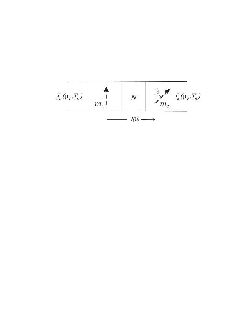
Figure 1: Schematic of a spin-valve structure connected to reservoirs at different chemical potentials and/or temperatures ($f_{L(R)}$ are the Fermi-Dirac distribution functions). Charge and heat flows through the normal metal spacer (N) are functions of the angle between the magnetization directions ($\theta$) in the ferromagnets.

In the following we explain the method, initially disregarding bulk impurity scattering, which is justified in the thin layer limit when interface scattering is dominant. We start with a simple normal metal $N_{1}|N|N_{2}$ trilayer structure in which metal $N$ is sandwiched between two electron reservoirs consisting of different metals $N_{1(2)}$. We then extend the methodology by making first one and then both reservoirs magnetic. In the $F_{1}|N|F_{2}$ (ferromagnet$|$normal-metal$|$ferromagnet) spin-valve sketched in Fig. 1, the relative orientation of the magnetization directions as well as the strength of the inelastic collisions become important parameters. Finally, we show how bulk impurity scattering (normal as well as spin-flip) can be introduced into the formalism, discuss the relevance of our results for experiments and finish with a summary and conclusions.

II Current-induced electron cooling and heating

A resistor network theory is an efficient way to describe the electric transport properties of magnetic heterostructures. Used to model the giant magnetoresistance effect in terms of the two-channel series resistor model, Valet and Fert (1993); Bass and Pratt Jr. (1999) it has been generalized to include the spin transfer torque in non-collinear magnetization configurations.Brataas et al. (2006) A resistor model for thermoelectric effects was introduced by MacDonaldMacDonald (1962) to understand the effects of different types of impurities in homogeneous bulk metals.

In the present section we develop a generalized (spin-less) circuit theory to describe the effects of temperature and voltage bias on normal metal heterostructures. Our starting point is a (non-unique) definition of the circuit or device topology by partitioning it into reservoirs, resistors and nodes. Discrete resistive elements are interfaces, potential barriers or constrictions that limit the transport. We require that these resistors can be represented by purely elastic scattering processes. The resistors are separated by nodes, in which electrons can be described by semiclassical distribution functions, $f_{i}$ in node $i$. When inelastic electron-electron or electron-phonon interactions in the nodes are strong enough, the $f_{i}$ become Fermi-Dirac distributions parametrized by temperatures $T_{i}$ and chemical potentials $\mu_{i}$. The charge and heat currents through a given resistor, denoted by $I=\int d\epsilon\imath(\epsilon)$ and $e\dot{Q}=\int d\epsilon(\epsilon-\mu)\imath(\epsilon)=eI^{E}-\mu I,$ respectively, where $\mu$ is the global chemical potential in equilibrium, are determined via the spectral current density

$$\imath(\epsilon)=G(\epsilon)[f_{L}(\epsilon)-f_{R}(\epsilon)],$$ (1)

where $G(\epsilon)$ is an energy-dependent (spectral) conductance between two neighboring nodes with distribution functions $f_{L(R)}$. According to Landauer-B$\ddot{\text{u}}$ttiker scattering theory the conductance

$$G(\epsilon)=\frac{2e^{2}}{h}\sum_{mn}[\delta_{mn}-r_{mn}^{\ast}(\epsilon)r_{mn}(\epsilon)].$$ (2)

depends on the energy-dependent reflection amplitudes $r_{mn}(\epsilon)$ at the resistor for electrons that are incident from a node or reservoir. $2e^{2}/h\simeq 1/13\operatorname{k\Omega}$ is the quantum of conductance. For structure elements such as interfaces which are not overly complicated, $r_{mn}(\epsilon)$ can be calculated from microscopic, first-principles calculations.Xia et al. (2006); Hatami et al. (2007); Zhang et al. (Unpublished) Thermoelectric effects arise from the energy dependence of $G(\epsilon)$. The circuit theory approach requires that scattering in the resistive elements is elastic. $G(\epsilon)$ may in principle be bias dependent, which becomes important for tunnel junctions. Here we concentrate on abrupt intermetallic interfaces with bias-independent spectral conductances. The interface resistance of transparent interfaces in a diffuse environment is affected by a correction caused by the drift of the distribution function.Schep et al. (1997); Brataas et al. (2006) The bare spectral resistance $G(\epsilon)^{-1}$ is then substituted by $G(\epsilon)^{-1}-\left[G_{N_{L}}(\epsilon)^{-1}+G_{N_{R}}(\epsilon)^{-1}\right]$, where $G_{N_{i}}(\epsilon)=2e^{2}M_{N_{i}}(\epsilon)/h$ are the Sharvin conductances of the metals that form the interface and $M_{N_{i}}$ are the total numbers of single-spin transport modes.

Let us now consider a non-equilibrium steady state in a simple $N_{1}|N|N_{2}$ normal metal structure in which the chemical potential $\mu_{1(2)}=\mu-eV_{1(2)}$ and temperature $T_{1(2)}$ of the nodes deviate from their equilibrium values $(\mu,T)$. Node $N$ is assumed to be fully thermalized with a distribution described by $(eV_{N},T_{N})$ that still have to be determined. To lowest order in the applied thermoelectric fields, we use the expansions $f_{i}\approx f_{0}+\frac{\partial f_{0}}{\partial\mu}(\mu_{i}-\mu)+\frac{\partial f_{0}}{\partial T}(T_{i}-T)$ in the following, where $f_{0}$ is the equilibrium Fermi-Dirac distribution function. It is possible to proceed and compute thermoelectric properties for arbitrary energy dependences of $G(\epsilon)$. However, results become much simpler upon using the Sommerfeld expansion Ashcroft and Mermin (1976) in $k_{B}T/\epsilon_{F}$. Provided the conductances do not vary too rapidly near the Fermi energy (to be precise $\partial_{\epsilon}G|_{\epsilon_{F}}\neq\infty$ and $G(\epsilon)e^{-\epsilon/k_{B}T}|_{\epsilon\gg\epsilon_{F}}\rightarrow 0$), the following approximation is applied

$$\int_{-\infty}^{\infty}d\xi\left(-\frac{\partial f_{0}}{\partial\xi}\right)\xi^{n}G(\xi)\approx G(0)\delta_{n,0}+\frac{\pi^{2}}{6}(k_{B}T)^{2}$$

$$\times\left[n(n-1)\xi^{n-2}G(\xi)+2n\xi^{n-1}\partial_{\xi}G(\xi)+\xi^{n}\partial^{2}_{\xi}G(\xi)\right]_{\xi=0}$$ (3)

where $\xi$ is the energy variable relative to the Fermi energy. Applying the Sommerfeld expansion to the expressions for the charge and heat currents in terms of the spectral current density, Eq.(1), results in expressions for the charge and heat currents into the normal node through junctions 1 and 2 , valid for $\frac{\pi^{2}}{6}(k_{B}T)^{2}\partial^{2}_{\epsilon}G|_{\epsilon_{F}}\ll G|_{\epsilon_{F}}$:

$$\left(\begin{array}[c]{c}I_{1(2)}\\ \dot{Q}_{1(2)}\end{array}\right)=G_{1(2)}\left(\begin{array}[c]{cc}1&S_{1(2)}\\ -S_{1(2)}T&-\mathcal{L}_{0}T\end{array}\right)\left(\begin{array}[c]{c}V_{N}-V_{1(2)}\\ T_{N}-T_{1(2)}\end{array}\right),$$ (4)

where $\mathcal{L}_{0}=(k_{B}/e)^{2}\pi^{2}/3\simeq 2.45\times 10^{-8}\mathrm{V}^{2}\mathrm{K}^{-2}$ is the Lorenz number. $G_{i}=G_{i}\left(\epsilon_{F}\right)$ are the conductances and $S_{i}=-e\mathcal{L}_{0}T\partial_{\epsilon}\ln G_{i}|_{\epsilon_{F}}$ (Mott’s formula) are the Seebeck coefficients or thermopowers at the zero-temperature chemical potential, which for metals is just the Fermi energy $\epsilon_{F}$. In bulk materials the thermopower can be positive or negative and even change sign as a function of the temperature.Colquitt, Jr. et al. (1971)

The chemical potential shift $eV_{N}$ and temperature $T_{N}$ of the central normal node and thus the thermal distribution function $f_{N}$ are determined by conservation laws: the charge and energy flows of the electrons are conserved, $I_{1}+I_{2}=0$ and $\dot{Q}_{1}+\dot{Q}_{2}=0$. The latter is affected in principle by the phonon heat conduction through the contacts (see Appendix A) but is disregarded here since thermal transport in good metals is dominated by the conduction electrons.Gundrum et al. (2005) Using Eq. (4) and the conservation laws we find to lowest order in the charge current $I$ that the electron temperature $T_{N}$ of the normal island is modified from the zero-charge current value $T_{0}$ as

$$T_{N}=T_{0}+\frac{(\Pi_{1}-\Pi_{2})I}{\kappa_{1}+\kappa_{2}},$$ (5)

The electron cooling or heating of asymmetric structures $(\Pi_{1}\neq\Pi_{2})$ by the applied current is the Peltier effect. $\Pi_{1(2)}=S_{1(2)}T$ are the Peltier coefficients and

$$\kappa_{1(2)}=\mathcal{L}_{0}TG_{1(2)}(1-S_{1(2)}^{2}/\mathcal{L}_{0})$$ (6)

are the thermal conductances of the resistive elements. Large thermopowers violate the simple proportionality between electrical and heat conductance, $\kappa=\mathcal{L}_{0}TG$, the Wiedemann-Franz law. The expression for the zero-current temperature in the central node

$$T_{0}=\frac{\kappa_{1}T_{1}+\kappa_{2}T_{2}}{\kappa_{1}+\kappa_{2}},$$ (7)

follows from energy conservation. The charge current $I=I_{\Delta V}+I_{\Delta T}$ is excited by a voltage difference $\Delta V=V_{2}-V_{1}$ as well as the temperature bias $\Delta T=T_{2}-T_{1}$. The total electric charge and heat currents are then given by,

$$I =\bar{G}(\Delta V+\bar{S}\Delta T)$$ (8)

$$\dot{Q} =-\bar{\Pi}I-\bar{\kappa}\Delta T,$$ (9)

where the total conductance becomes

$$\bar{G}=\frac{G_{1}G_{2}(\kappa_{1}+\kappa_{2})}{G_{1}\kappa_{1}+(G_{1}+G_{2})\kappa_{12}+G_{2}\kappa_{2}}$$ (10)

with

$$\kappa_{12}\equiv 2\mathcal{L}_{0}T~{}\frac{G_{1}G_{2}}{G_{1}+G_{2}}\left(1-\frac{S_{1}S_{2}}{\mathcal{L}_{0}}\right).$$ (11)

The total conductance/resistance ($\bar{R}=1/\bar{G}$) violates the series resistor rule, $\bar{R}\neq R_{1}+R_{2}$ $\left(\text{with }R_{i}=1/G_{i}\right)$, which is only recovered when either $S_{1}=S_{2}$ or when $S_{i}^{2}\ll\mathcal{L}_{0}$; the latter is always the case at low temperatures. On the other hand, the total thermopower $\bar{S}$ (or Peltier coefficient $\bar{\Pi}=\bar{S}T$) and thermal conductance $\bar{\kappa}$ do obey simple sum rules

$$\frac{\bar{S}}{{\bar{\kappa}}} =\frac{S_{1}}{\kappa_{1}}+\frac{S_{2}}{\kappa_{2}},$$ (12)

$$\frac{1}{{\bar{\kappa}}} =\frac{1}{\kappa_{1}}+\frac{1}{\kappa_{2}}.$$ (13)

When in series, two thermal or electrical resistances are additive, as expressed in Eq. (13) or $\bar{R}=R_{1}+R_{2}$ which is valid in the limit $S_{i}^{2}\ll\mathcal{L}_{0}$. In contrast, the thermopower, Eq. (12), depends on the spatial distribution of the scattering objects rather than its integral (the thermopower in a homogeneous bulk metal does not depend on its length). Equation (12) holds not only for the spatially distributed scatterers considered here, but can also describe the relative contributions of different types of scatterers to the thermopower in bulk materials.MacDonald (1962)

The second law of thermodynamics (a non-negative entropy production) requires $\kappa>0$, which in the Sommerfeld approximation leads toGuttman et al. (1995) $|S_{max}|=\sqrt{\mathcal{L}_{0}}\simeq 157\operatorname{\mu V}\mathrm{/}\mathrm{\operatorname{K}}$. Defining the thermoelectric figure of merit $ZT=|{\bar{S}}\Delta T_{N}/\Delta V|$, Eq. (5) for the temperature change $\Delta T_{N}=T_{N}-T_{0}$ induced by an applied voltage results in

$$ZT=\frac{1}{4}\left|\frac{\bar{S}(S_{1}-S_{2})}{\mathcal{L}_{0}-\bar{S}^{2}}\right|$$ (14)

assuming $G_{1}=G_{2}$ and $\left(S_{1}-S_{2}\right)S_{1(2)}\ll\mathcal{L}_{0},$ so that $|\bar{S}_{max}|=\sqrt{\mathcal{L}_{0}}$ corresponds to the maximum efficiency $ZT=\infty$. Even for the best thin film thermoelectric materialsSales (2002) $ZT\lessapprox 3$, and for most metallic structures $S^{2}\ll\mathcal{L}_{0}$. Quantum point contacts, however, have larger thermopowers due to size quantization,Molenkamp et al. (1992); van Houten et al. (1992) so $S^{2}$ can be comparable to $\mathcal{L}_{0}$ and the predicted effects should be observable in nanoscale structures.

Equation (5) holds for low current densities, for which $\delta V/2\ll\Pi\ll 2\mathcal{L}_{0}T^{2}/\delta V,$ where $\delta V$ is the voltage drop over a single contact. Non-linear heating by applied currents can be included my means of the quadratic term in the expansions of the distribution functions, i.e. $f_{i}\approx f_{0}+\frac{\partial f_{0}}{\partial\mu}(\mu_{i}-\mu)+\frac{\partial f_{0}}{\partial T}(T_{i}-T)+\frac{1}{2}\frac{\partial^{2}f_{0}}{\partial\mu^{2}}(\mu_{i}-\mu)^{2}+...$, and using the approximation $\int_{-\infty}^{\infty}d\xi\left(\frac{\partial^{2}f_{0}}{\partial\xi^{2}}\right)\xi G(\xi)\approx G(0)$. When $\Pi\ll\delta V\ll\mathcal{L}_{0}T^{2}/\Pi$, expressions for the nonlinear currents reduce to

$$\left(\begin{array}[c]{c}I_{1(2)}\\ \dot{Q}_{1(2)}\end{array}\right)\simeq G_{1(2)}\left(\begin{array}[c]{cc}1&S_{1(2)}\\ -\Pi_{1(2)}-\tilde{V}_{1(2)}&-\mathcal{L}_{0}\tilde{T}_{1(2)}\end{array}\right)$$ (19)

$$\times\left(\begin{array}[c]{c}V_{N}-V_{1(2)}\\ T_{N}-T_{1(2)}\end{array}\right),$$ (22)

where $\tilde{V}_{1(2)}=(V_{N}+V_{1(2)})/2$ and $\tilde{T}_{1(2)}=(T_{N}+T_{1(2)})/2$. For reservoir temperatures $T_{1}=T_{2}=T$ and in the absence of the thermopowers $S_{1(2)}=0$, or when Joule heating dominates, particle and energy current conservation requires $(G_{1}+G_{2})V_{N}=G_{1}V_{1}+G_{2}V_{2}$ and

$$T_{N}^{2}=T^{2}+\frac{(\Delta V)^{2}}{\mathcal{L}_{0}}\frac{G_{1}G_{2}}{(G_{1}+G_{2})^{2}},$$ (23)

so that we recover the result for the maximum amplitude of the electron temperature profile in the middle of a diffusive bulk wire (with the conductance $G_{1}=G_{2}=G$) due to heating by inelastic electron-electron collisions.Nagaev (1995); Pothier et al. (1997) By taking into account the thermopowers of the junctions, but in the limit $S^{2}\ll\mathcal{L}_{0}$, the change in the electron temperature in the island is found as

$$\Delta T_{N}=\frac{(\Pi_{1}-\Pi_{2})I}{\mathcal{L}_{0}T(G_{1}+G_{2})}+\frac{\bar{R}I^{2}}{2\mathcal{L}_{0}T(G_{1}+G_{2})}$$

$$+\mathcal{O}\left(\left(\frac{\Delta T}{T}\right)^{2},\frac{\Delta T}{T}\frac{(\Delta V)^{2}}{\mathcal{L}_{0}T^{2}},\frac{S(\Delta V)^{3}}{\mathcal{L}_{0}^{2}T^{3}},\cdots\right).$$ (24)

in which the electric current Eq. (8) is driven by a voltage and/or temperature bias. Equations (23) and (24) yield the same result for a small temperature increase due to Joule heating when $\Pi_{1}=\Pi_{2}$ and $T_{1}=T_{2}$.

Following Fukushima et al.Fukushima et al. (2005a, b) we use Eq. (24) to derive an expression for the Peltier coefficient in terms of a critical current $I_{p}$ at which heating and cooling cancel each other. Assuming that the resistance scales linearly with the electron temperature in the node, $\Delta T_{N}=0$ leads to

$$(\Pi_{2}-\Pi_{1})I_{p}=\frac{\bar{R}I_{p}^{2}}{2}.$$ (25)

The factor 1/2 on the right hand side implies that the current heating is only half as large as considered by Refs. Fukushima et al., 2005a and Fukushima et al., 2005b, whereas the “cooling power” $\bar{R}I_{p}=2(\Pi_{2}-\Pi_{1})$ (in units of mV) is twice as large. This discrepancy can be explained as follows. In our model, the energy is dissipated in the nodes and reservoirs of the device, not at the sharp interfaces. We monitor the temperature change in the normal metal node which is assumed to be effectively thermalized. Half of the generated heat is dissipated in the reservoirs that by definition do not contribute to the resistance change. The expressions of Fukushima et al.Fukushima et al. (2005a, b) can be recovered by treating the highly resistive junctions in their samples as bulk material in which heat is generated and contributes to its temperature and resistance rise (see Section VII).

III Peltier and Seebeck effects in the presence of a single ferromagnetic element

The thermoelectric transport Eq. (4) can be generalized to include the spin degree of freedom. For spin-dependent thermoelectric transport through an $F|N$ interface the spin-polarized electric charge and heat currents read

$$\left(\begin{array}[c]{c}I^{\uparrow(\downarrow)}\\ \dot{Q}^{\uparrow(\downarrow)}\end{array}\right)=G^{\uparrow(\downarrow)}\left(\begin{array}[c]{cc}1&S^{\uparrow(\downarrow)}\\ -S^{\uparrow(\downarrow)}T&-\mathcal{L}_{0}T\end{array}\right)\left(\begin{array}[c]{c}V_{N}^{\uparrow(\downarrow)}-V_{F}^{\uparrow(\downarrow)}\\ T_{N}^{\uparrow(\downarrow)}-T_{F}^{\uparrow(\downarrow)}\end{array}\right),$$ (26)

where the spin-dependence of the conductance $G^{\uparrow(\downarrow)}$, thermopower $S^{\uparrow(\downarrow)}=-e\mathcal{L}_{0}T\partial_{\epsilon}\ln G^{\uparrow(\downarrow)}|_{\epsilon_{F}}$, heat current, and temperature is expressed by the superscript $\uparrow(\downarrow)$ for majority (minority) spin electrons. $V_{s}=V^{\uparrow}-V^{\downarrow}\$ is the particle spin accumulation. Referring to the discussion below we conjecture the existence of a heat spin accumulation $T_{s}=T^{\uparrow}-T^{\downarrow}$, i.e., a temperature imbalance for majority and minority electrons, when thermalization is weak. We also define the total thermopower $S=-(\Delta V/\Delta T)_{I=0}$ of an interface between a normal metal and a ferromagnet as

$$S=-e\mathcal{L}_{0}T\left(\frac{\partial_{\epsilon}G}{G}\right)_{\epsilon_{F}}=\left(\frac{G^{\uparrow}S^{\uparrow}+G^{\downarrow}S^{\downarrow}}{G^{\uparrow}+G^{\downarrow}}\right)_{\epsilon_{F}}.$$ (27)

This thermopower is observable when the interface is part of a (hetero) Sharvin point contact in direct contact with large reservoirs that prevent build-up of a spin accumulation. In a diffusive environment, however, the local spin accumulation should be taken into account, as described in the following. The spin-polarization of the interface thermopower is defined as

$$P_{S}\equiv\frac{S^{\uparrow}-S^{\downarrow}}{S^{\uparrow}+S^{\downarrow}}=\frac{P^{\prime}-P}{1-P^{\prime}P}$$ (28)

where $P$ and $P^{\prime}$ are the polarizations of the conductance $G^{\uparrow(\downarrow)}$ and its energy derivative $\partial_{\epsilon}G^{\uparrow(\downarrow)}$ respectively, both at the Fermi energy. Whereas $\left|P\right|<1,$ $\left|P^{\prime}\right|\gg 1$ when $\partial_{\epsilon}G^{\uparrow}$ approaches $-\partial_{\epsilon}G^{\downarrow}$. $P_{S}$ is also in principle unbounded. Using

$$-e\mathcal{L}_{0}T\left(\frac{\partial P}{\partial\epsilon}\right)_{\epsilon_{F}}=S(P^{\prime}-P)_{\epsilon_{F}},$$ (29)

it follows that $P_{S}\neq 0$ when the conductance polarization is energy dependent. Spin-polarization of the thermopower of ferromagnetic materialsCadeville and Roussel (1971); Piraux et al. (1992); Shi et al. (1996) has been invoked to, e.g., explain the giant magneto-thermoelectric effect of magnetic multilayers.Gravier et al. (2004) For a few combinations of materials, the interface thermopower and its spin polarization are known from first principles calculations.Hatami et al. (2007); Zhang et al. (Unpublished)

Consider now an $F_{1}|N|N_{2}$ pillar with one magnetic contact. Conservation of charge, spin and energy currents implies the Kirchhoff rules $I_{1\alpha}+I_{2\alpha}=0$ and $\sum_{\alpha}\dot{Q}_{1}^{\alpha}+\dot{Q}_{2}^{\alpha}=0,$ where $\alpha=\uparrow\left(\downarrow\right)$. The individual spin currents are separately conserved since we disregard spin-flip scattering in the normal metal spacer when the length of the metal does not exceed its spin diffusion length. In contrast, the heat spin accumulation, i.e. the temperature difference between the two spin species on the central island, is assumed to vanish by strong inelastic scattering, which is likely for temperatures which are not too low and/or metals which are not too clean. In this regime the electron temperature on the island becomes

$$T_{N}=T_{0}+\frac{(\gamma_{1}S_{1}-S_{2})I}{\mathcal{L}_{0}(G_{1}+G_{2})}.$$ (30)

We may call

$$\gamma_{1}=\frac{(1-P^{\prime}P)+G_{2}/G_{1}}{(1-P^{2})+G_{2}/G_{1}}.$$ (31)

a ”spin-entropy factor”, because it reflects the spin-polarization of the entropy flow per unit of the electric current (the thermopower), $S^{\uparrow}\neq S^{\downarrow}$ ($P^{\prime}\neq P$). In the limit $S_{\uparrow(\downarrow)}^{2}\ll L_{0}$ (and therefore $\kappa^{\uparrow(\downarrow)}\approx L_{0}TG^{\uparrow(\downarrow)}$) the temperature $T_{0}$ (Eq. (7)) is not affected by the magnetism. When $P^{\prime}\neq P$ the Peltier cooling (heating) does not vanish even when $S_{1}=S_{2}$. The thermopower spin polarization, $P_{S}$, can enhance or suppress the Peltier effect depending on the spin polarization $P$ and the relative amplitude of the conductances $G_{2}/G_{1}$. $\gamma_{1}$ can become large when $\left|P^{\prime}\right|\gg 1$ (an example is $P^{\prime}$ at a disordered Cr$|$Fe interface, see Table. I).

The total thermopower can be expressed in terms of the properties of its constituent elements, in the limit $S^{\uparrow(\downarrow)}\ll\sqrt{\mathcal{L}_{0}}$ and for strongly thermalized electrons, as

$$\frac{\bar{S}}{\bar{G}}=\frac{\gamma_{1}S_{1}}{G_{1}}+\frac{S_{2}}{G_{2}}.$$ (32)

Therefore, when a spin accumulation is excited in the proximate normal metal, the magnetic junction contributes to the thermopower not by the Seebeck coefficient of the point contact $S_{1},$ but by the product with the spin-entropy factor $\gamma_{1}S_{1}$.

IV Magneto-Peltier and magnetothermopower in spin valves

We proceed to the study of thermoelectric effects in asymmetric $F_{1}\left(\mathbf{m_{1}}\right)|N|F_{2}\left(\mathbf{m_{2}}\right)$ spin valves (see Fig. 1) for arbitrary relative orientations of the magnetizations, $\mathbf{m_{1}}\cdot\mathbf{m_{2}}=\cos\theta$. The electron distributions in the nodes and reservoirs are now $2\times 2$ matrices in spin space that can be expanded into scalar and vector components $\hat{f}^{F(N)}=f_{c}^{F(N)}\hat{1}+\hat{\mbox{\boldmath$\sigma$}}\cdot\mathbf{s}^{F(N)}f_{s}^{F(N)}$, where $\hat{\mbox{\boldmath$\sigma$}}$ is the vector of Pauli matrices and $\hat{1}$ the $2\times 2$ unit matrix. The unit vector of the spin quantization axis $\mathbf{s}^{F}$ is parallel to the magnetization of the ferromagnet, whereas $\mathbf{s}^{N}$ can point in any direction. In linear response, the $2\times 2$ spectral current in spin space across a ferromagnet-normal metal junction at energy $\epsilon$ in the absence of spin-flip and inelastic interface scattering is given as a spectral Landauer-Büttiker-like expressionBrataas et al. (2006, 2000, 2001)

$$\hat{\imath}_{N|F}\left(\epsilon\right)=\sum_{\alpha\beta}G^{\alpha\beta}\left(\epsilon\right)\hat{u}^{\alpha}[\hat{f}^{F}\left(\epsilon\right)-\hat{f}^{N}\left(\epsilon\right)]\hat{u}^{\beta},$$ (33)

where $\hat{u}^{\uparrow(\downarrow)}=(\hat{1}\pm\hat{\mbox{\boldmath$\sigma$}}\mathbf{\cdot m})/2$ are projection matrices in which the unit vector $\mathbf{m}\equiv\mathbf{s}^{F}$ denotes the magnetization direction of the ferromagnet. The conductance tensor elements read $G^{\alpha\beta}\left(\epsilon\right)=\left(e^{2}/h\right)\sum_{nm}[\delta_{mn}-r_{nm}^{\alpha}\left(\epsilon\right)(r_{nm}^{\beta}\left(\epsilon\right))^{\ast}]$ in terms of the energy-dependent reflection coefficients $r_{nm}^{\alpha}(\epsilon)$ for majority and minority spins at the $N|F$ interface. Its diagonal elements are the conventional spin-dependent conductances that govern, e.g., the giant magnetoresistance, whereas the complex non-diagonal elements, the so-called spin-mxing conductances, parameterize the transverse spin currents that are absorbed by the ferromagnet and give rise to torques on the magnetization. The total charge-spin and heat matrix currents are defined as $\hat{I}=\int d\epsilon\;\hat{\imath}(\epsilon)$ and $e\hat{\dot{Q}}=\int d\epsilon(\epsilon-\mu)\hat{\imath}(\epsilon)=e\hat{I}^{\epsilon}-\mu\hat{I},$ respectively, where $\mu$ is the equilibrium chemical potential and $\hat{I}^{\epsilon}$ the energy current. In the following we assume that both spin components $f^{\uparrow(\downarrow)}=f_{c}\pm f_{s}$ of the diagonalized matrix distribution functions $\hat{f}^{F(N)}$ may be described by thermal-equilibrium Fermi-Dirac distribution functions with spin-dependent chemical potentials and temperatures. The Sommerfeld expansion can then be employed to derive expressions for the transport currents as a function of applied voltage or temperature gradients in terms of the conductance tensor $G^{\alpha\beta}$ and its energy derivative $G_{\epsilon}^{\alpha\beta}\$at the Fermi energy.Hatami et al. (2007) The total charge, spin and heat currents read $I_{c}=\mathrm{Tr}[\hat{I}],$ $\mathbf{I}_{s}=\mathrm{Tr}[\mbox{\boldmath$\sigma$}\hat{I}]$ and $\dot{Q}_{c}=\mathrm{Tr}[{\hat{\dot{Q}}}],$ respectively, where the trace is over spin indices.

The charge and energy conservation laws read $I_{c1}+I_{c2}=0$ and $\dot{Q}_{c1}+\dot{Q}_{c2}=0$. Moreover, in the absence of spin-flip scattering in the normal node, the total spin angular momentum current is conserved as well, i.e., $\mathbf{I}_{s1}+\mathbf{I}_{s2}=0$. These Kirchhoff Laws close the system of transport equations in the strongly thermalized regime. In what we call the weakly thermalized regime, the distributions for each spin species are thermalized separately, but the energy exchange between the spin subsystems is disregarded, which is a realistic scenario at low temperatures.Hatami et al. (Unpublished) In this limit a spin temperature vector on the central island exists, $\mathbf{T}_{s}\neq 0,$ and we require $\mathbf{\dot{Q}}_{s1}+\mathbf{\dot{Q}}_{s2}\approx 0$ where $\mathbf{\dot{Q}}_{s}=\mathrm{Tr}[\mbox{\boldmath$\sigma$}\hat{\dot{Q}}]$, which means that energy is conserved for each spin channel separately. It is worth while to compare the thermoelectric transport properties such as the total conductance and thermopower of the spin-valve structure in the different interacting regimes.

In the strongly thermalized regime for a symmetric spin-valve, $G_{1}^{\alpha\beta}=G_{2}^{\alpha\beta}$ and $G_{\epsilon 1}^{\alpha\beta}=G_{\epsilon 2}^{\alpha\beta},$ the temperature of the normal metal island $T_{N}=T_{0}$ is not affected by electric current. The total electric current readsHatami et al. (2007)

$$I_{c}=\frac{G}{2}\left(\Delta V+S\Delta T\right)-\frac{PG}{2}\frac{\tan^{2}\theta/2}{\eta_{R}+\tan^{2}\theta/2}\left(P\Delta V+P^{\prime}S\Delta T\right).$$ (34)

Here $\eta_{R}=2\operatorname{Re}G^{\uparrow\downarrow}/G>0,$ where $G^{\uparrow\downarrow}$ is the complex spin mixing conductance.Brataas et al. (2006) For most metallic contacts $\eta_{I}=2\operatorname{Im}G^{\uparrow\downarrow}/G,$ is small ($\eta_{I}\ll\eta_{R}$) Zwierzycki et al. (2005) and is disregarded in the analytical results. However, since $\eta_{I}$ is not small for $\text{Cr}|\text{Fe}$ and $\text{Cr}|\text{Co}$ interfaces, see Table I, it is included in the numerical results for these junctions. The angular magneto-resistance for $\Delta T=0$ as measured by Urazhdin et al.S. Urazhdin and Pratt, Jr. (2005) is well described by circuit theory.Kovalev et al. (2006) The thermoelectric transport properties of the spin-valve structure differ significantly in the different interacting regimes. In the Sommerfeld approximation, the spin-mixing thermopower $S^{\uparrow\downarrow}\equiv-e\mathcal{L}_{0}TG_{\epsilon}^{\uparrow\downarrow}/G^{\uparrow\downarrow}$ and the dimensionless mixing parameter $\eta_{R(I)}^{\prime}\equiv 2\operatorname{Re}(\operatorname{Im})G^{\uparrow\downarrow}_{\epsilon}/G_{\epsilon}$ enter expressions for the electric currents only when ${\bf T}_{s}^{N}\neq 0$, i.e. in the weakly thermalized regime.Hatami et al. (2007)

	$G(10^{15}\operatorname{\Omega}^{-1}\operatorname{m}^{-2})$	$S/T$($\operatorname{nV}/\operatorname{K}^{2}$)	$P(\%)$	$P^{\prime}(\%)$	$P_{S}(\%)$	$\eta_{R}$	$\eta_{I}$	$\eta_{R}^{\prime}$	$\eta^{\prime}_{I}$
Cu$|$Co(001)	4.43	-13	75	72	-8	0.50	-0.036	0.03	0.00
Cu$|$Co(001)*	4.29	-34	74	89	43	0.49	-0.054	0.06	-0.01
Cu$|$Co(110)	3.42	-10	69	6	-66	0.67	-0.082	-0.32	0.44
Cu$|$Co(110)*	3.52	-13	64	85	45	0.63	-0.077	0.07	-0.05
Cu$|$Co(111)	3.69	-15	60	56	-6	0.53	-0.006	0.13	0.48
Cu$|$Co(111)*	3.42	-15	68	77	17	0.64	-0.073	0.13	-0.05
Cr$|$Au(001)	0.36	7	0	0	0	$-$	$-$	$-$	$-$
Cr$|$Au(001)*	0.67	0	0	0	0	$-$	$-$	$-$	$-$
Cr$|$Fe(001)	0.88	22	-74	-40	48	4.23	1.38	-4.27	-1.38
Cr$|$Fe(001)*	0.94	7	-53	-190	-9500	3.25	0.43	-0.48	9.39
Cr$|$Co(001)	0.56	62	-62	-111	-160	3.03	-0.59	-2.86	-3.46
Cr$|$Co(001)*	0.71	23	-23	-95	-92	2.92	-1.79	-0.86	3.21

Table 1: Thermoelectric interface parameters calculated at the Fermi energy for a number of almost lattice-matched interfaces including Schep’s drift correction.Schep et al. (1997) With the exception of the Cr$|$Co interface for which Co is assumed to be bcc, Cr and Fe are bcc while Cu, Co and Au are assumed to be fcc. The asterisk * indicates a dirty interface modeled in a 10x10 lateral supercell with two layers of 50%-50% alloy.

In the presence of a temperature bias $\Delta T$ with an open electric circuit ($I_{c}=0)$, the induced thermoelectric voltage $\Delta V$ is described by the angular magnetothermopower (MTP) $\bar{S}(\theta)=-\left(\Delta V/\Delta T\right)_{I_{c}=0}$ which in the strongly thermalized regime reads Hatami et al. (2007)

$$\frac{\bar{S}(\theta)}{S}=\frac{\eta_{R}+(1-PP^{\prime})\tan^{2}\theta/2}{\eta_{R}+(1-P^{2})\tan^{2}\theta/2},\$$ (35)

$$MTP\equiv\frac{\bar{S}(\pi)-\bar{S}(0)}{S}=\frac{-PP_{S}}{1+PP_{S}}.$$ (36)

The MTP is finite when the interface thermopower is spin polarized, $P_{S}\neq 0$. When $PP^{\prime}>1$ (which also requires $P_{S}<0$) one finds an angle $\theta_{0}=2\tan^{-1}\sqrt{\eta_{R}/(PP^{\prime}-1)}$ where the thermoelectric power can change sign, i.e. a spin-valve with non-collinear magnetic configuration can display a transition from electron-like to hole-like transport. In a spin-valve the thermally induced charge-currents that enter the normal node from both sides can be made to cancel such that the net thermoelectric voltage vanishes, ${\bar{S}}=0$. Note that not only the individual spin currents but also the charge current depend on the effective spin polarizations. The MTP vanishes in the half-metallic limit $P=P^{\prime}=\pm 1$.

In the weakly thermalized regime on the other hand, the magnetothermopower Eq. (36) is twice as large, whereas the magnetoresistance and $\bar{S}(0)$ do not change (in the limit $S^{2}\ll\mathcal{L}_{0}$). $\bar{S}(\pi)$ is enhanced in this case because the heat spin accumulation facilitates the thermoelectric voltage build-up. In this regime an angular magnetothermopower is found even when $P_{S}=0$ provided that $\eta_{R}^{\prime}\equiv 2\operatorname{Re}\partial_{\epsilon}G^{\uparrow\downarrow}/\partial_{\epsilon}G\neq\eta_{R}$, , which is destroyed by full thermalization.

The Onsager-Kelvin relation between the total Seebeck and Peltier coefficients in spin valves, i.e. ${\bar{\Pi}}(\theta)={\bar{S}}(\theta)T$ in which ${\bar{\Pi}}\equiv\left(-{\dot{Q}}_{c}/I_{c}\right)_{\Delta T=0}$, is found to hold in both thermalization regimes.

For a quantitative analysis we need to know more about the thermoelectric parameters for interfaces. In the absence of experimental estimates, we calculated the parameters from first-principles within the framework of density functional theory for a number of interfaces which figure prominently in the field of magnetoelectronics.Hatami et al. (2007) The values are given in Table 1. For an A$|$B interface, the calculation proceeds as follows.Xia et al. (2006); Zwierzycki et al. (2008) Self-consistent density functional theory calculations are first performed separately for bulk A and B materials. These calculations yield bulk charge- and spin- densities and potentials, and the corresponding Fermi energies. A self-consistent interface calculation is next performed subject to the potentials (and densities) far from the interface being equal to their bulk values, up to a constant which is adjusted so as to equalize the Fermi energies.Turek et al. (1997) The interface breaks the lattice periodicity perpendicular to the interface leaving only two-dimensional periodicity parallel to the interface that is characterized by the two-dimensional Bloch vector $\mathbf{k}_{\parallel}$. The electronic structure of the localized perturbation formed by the interface is handled using a Green’s function method, a so-called “Surface Green’s Function”. The rank of the matrix of the perturbation is made finite and minimized by making use of the translational symmetry parallel to the interface and using a maximally-localized basis of tight-binding (TB) muffin-tin orbitals (MTOs).Andersen and Jepsen (1984); Andersen et al. (1986) To calculate the scattering matrix $\mathcal{S}$

$$\mathcal{S}(\mathbf{k}_{\parallel},\epsilon)\equiv\left(\begin{array}[c]{cc}r(\mathbf{k}_{\parallel},\epsilon)&t^{\prime}(\mathbf{k}_{\parallel},\epsilon)\\ t(\mathbf{k}_{\parallel},\epsilon)&r^{\prime}(\mathbf{k}_{\parallel},\epsilon)\end{array}\right),$$ (37)

at real energies (at or close to the Fermi energy in the context of transport), we use a wave-function-matching scheme due to AndoAndo (1991) which involves the calculation of individual scattering states far from the interface. The rank of the reflection and transmission matrices $r,r^{\prime},t,t^{\prime}$ is determined by the number of Bloch states at a given energy $\epsilon$ and transverse wave-vector $\mathbf{k}_{\parallel}$. The minimal TB-MTO basis is very efficient and makes it possible to model incommensurate lattices and various types of disorder using large lateral supercells.Xia et al. (2001, 2006); Zwierzycki et al. (2008) Substitutional disorder where one or more layers of atoms form an alloy is conveniently treated by calculating the potentials self-consistently using a layer versionTurek et al. (1997) of the coherent potential approximationSoven (1967) and then distributing at random the site potentials in lateral supercells subject to maintenance of the appropriate layer concentrations.Xia et al. (2006) The mixing conductance is most easily calculated in terms of the reflection matrices.Xia et al. (2002); Zwierzycki et al. (2005) We consider here interfaces in diffuse metallic systems which implies that we have to use a generalization of the Schep correctionSchep et al. (1997); Brataas et al. (2006) by replacing the bare $G^{\alpha\beta}(\epsilon)^{-1}$ with $G^{\alpha\beta}(\epsilon)^{-1}-\left[G_{\mathrm{N}}(\epsilon)^{-1}+\delta_{\alpha\beta}G^{\alpha}_{\mathrm{F}}(\epsilon)^{-1}\right]$, where $G_{\mathrm{N}}(\epsilon)=e^{2}M_{\mathrm{N}}(\epsilon)/h$ and $G^{\alpha}_{\mathrm{F}}(\epsilon)=e^{2}M^{\alpha}_{\mathrm{F}}(\epsilon)/h$ are the single-spin Sharvin conductances of the normal and ferromagnetic metals forming the interface. The thermopower and other generalized thermoelectric parameters are determined by numerically differentiating the scattering matrix calculated as a function of the energy. Details of the numerical procedures will be given in a separate paper.Zhang et al. (Unpublished)

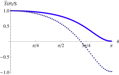
Figure 2: Magnetothermoelectric power as a function of relative angle between the magnetizations in a $\mathrm{Fe}\mathrm{|Cr|Fe}$ (001) spin valve with dirty interfaces. The MTP is significantly different for the strong (full line) and weak (dotted line) thermalization in the normal metal spacer.

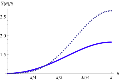
Figure 3: Same as Fig. 2 but for a $\mathrm{Co|Cu|Co}$ (110) spin valve with clean interfaces.

We use the data in Table I to compute the angular dependence of the thermoelectric properties of a few spin valves for illustrative purposes. Spin-flip scattering is disregarded here but will be discussed in later sections.

We plot the angular MTP for a Fe$|$Cr$|$Fe (001) spin valve with dirty interfaces in Fig. 2 and for a Co$|$Cu$|$Co (110) spin valve with clean interfaces in Fig. 3. The angular MTP is enhanced in the weakly thermalized regime (shown by dotted lines) by up to a factor of two for the antiparallel configuration. Depending on $P$ and $P_{S}$, the MTP can be of any sign, see Eq. (36).

We now turn to the Peltier effect of asymmetric spin valves. In the strongly thermalized regime and for $P_{S_{1}}=P_{S_{2}}=0,$ the Peltier cooling retains the simple form for normal metal structures, Eq. (5), whereas the total charge current is a complicated function of the magnetic configuration of the system. A magneto-Peltier effect (MPE), i.e., a dependence of the cooling power on the magnetic configuration, is found when the thermopower is spin dependent. For a voltage-biased spin valve with thermal asymmetry $S_{1}\neq S_{2}$ and $P_{1}^{\prime}\neq P_{2}^{\prime},$ but $G_{1}=G_{2}=G$, $P_{1}=P_{2}=P,$ and $S^{\uparrow(\downarrow)}_{i}\ll\sqrt{\mathcal{L}_{0}}$, we find for the temperature change of the normal metal spacer

$$\Delta T_{N}=\frac{(\gamma^{\text{MP}}_{1}S_{1}-\gamma^{\text{MP}}_{2}S_{2})I_{c}}{2\mathcal{L}_{0}G},$$ (38)

where the spin-entropy factors

$$\gamma_{1(2)}^{\text{MP}}\left(\theta\right)=\frac{(1-P_{1(2)}^{\prime}P)\tan^{2}\theta/2+\eta_{R}}{(1-P^{2})\tan^{2}\theta/2+\eta_{R}}$$ (39)

depend now on the magnetic configuration ($P^{\prime}_{1(2)}\neq P$). $\gamma_{1(2)}^{\text{MP}}=1$ and $\left(1-P_{1(2)}^{\prime}P\right)/\left(1-P^{2}\right),$ respectively, for parallel and antiparallel configurations. The MPE should therefore be observable in R vs. I curves of spin valves during current-induced magnetization reversal. According to Eq. (25) with $\bar{R}(I=I_{p})=\bar{R}(I=0)\equiv R_{0},$ the temperature change $\Delta T_{N}=T_{N}(\theta)-T_{0}$ corresponds to the cooling-power $R_{0}I_{p}\approx 2\mathcal{L}_{0}(G_{1}+G_{2})T\Delta T_{N}/I_{p}$ such that

$$R_{0}\left[I_{p}(\pi)-I_{p}(0)\right]=$$

$$4\frac{G_{1}P_{2}(P_{1}^{\prime}-P_{1})\Pi_{1}-G_{2}P_{1}(P_{2}^{\prime}-P_{2})\Pi_{2}}{G_{1}(1-P_{1}^{2})+G_{2}(1-P_{2}^{2})}$$ (40)

This signal contains unique information on the spin-polarization of the thermopower. When thermalization is weak a MPE arises even when $P_{S_{1}}=P_{S_{2}}=0$ ($P^{\prime}_{1(2)}=P_{1(2)}$). A sign change in the cooling-power is also expected. In the strongly thermalized regime this arises from different angular dependences of the spin-entropy factors. When the effective thermopowers are equal, $\gamma^{\text{MP}}_{1}(\theta_{0})S_{1}=\gamma^{\text{MP}}_{2}(\theta_{0})S_{2}$, no Peltier cooling is expected, $R_{0}I_{p}(\theta_{0})=0$.

In Figs. 4 and 5, we illustrate the magneto-Peltier cooling by computing the angular dependent cooling-power $R_{0}I_{p}(\theta)$, at room temperature, for a hypothetical bcc Co$|$Cr$|$Fe (001) spin-valve structure with clean interfaces and for an asymmetric Co$|$Cu$|$Co (001) with one ideal and one disordered interface, using parameters from Table I. For comparison, we include the results in the weakly thermalized regime, depicted in the figures by dotted lines. The dependence of the Peltier cooling on the magnetic configuration observed in Fig. 4 for the Co$|$Cr$|$Fe spin-valve is caused by the relatively large values of the interface thermopower parameters $P$ and $P^{\prime}$. The relatively weak magneto-Peltier signal, $R_{0}[I_{p}(\pi)-I_{p}(0)]$ vanishes when $G_{1}=G_{2}$ and $P_{1}=P_{2}$, for weakly thermalized electrons (dotted line) is strongly enhanced by the inter-spin energy exchange in the opposite limit. The MPE for the asymmetric Co$|$Cu$|$Co (001) structure, Fig. 5, displays similar effect but with smaller amplitudes. For the strongly thermalized electron case, the MPE caused by interface scattering, $R_{0}[I_{p}(\pi)-I_{p}(0)]$, is of the order of $1-10{\rm mV}$, which is smaller than the experimental valuesFukushima et al. (2005a, b) $R_{0}I_{p}\approx 20-40{\rm mV}$. For a typical current density of $10^{8}{\rm A/cm}^{2}$, we find a maximum temperature drop $\Delta T_{N}(\theta)\approx 0.15{\rm K}$ which is also too small to explain experiments. Note that in the above we have assumed that interface scattering is dominant. As explained in the next sections, we show that these numbers are increased by including scattering in the bulk.

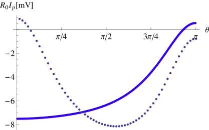
Figure 4: Magneto-Peltier cooling as a function of the angle between the magnetizations in the hypothetical bcc $\mathrm{Co|Cr|Fe}$ (001) spin valve. $R_{0}I_{p}(\theta)$ is the cooling power which compensates local Joule heating. The signal $R_{0}[I_{p}(\pi)-I_{p}(0)]$ is significantly different for strong (full line) and weak (dotted line) thermalization in the normal metal spacer.

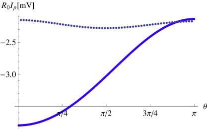
Figure 5: As Fig. 4 but for an asymmetric $\mathrm{Co}|\mathrm{Cu}|\mathrm{Co}$ (001) spin valve with one clean and one disordered interface.

The magneto-Peltier effect vanishes for symmetric spin-valve structures. Introducing the asymmetry $G_{1}\neq G_{2},$ we obtain an angle-dependent temperature modulation

$$\mathcal{L}_{0}\Delta T_{N}(\theta)=$$

$$\frac{2\left(G_{1}-G_{2}\right)P\left(P^{\prime}-P\right)SI_{c}\sin^{2}\frac{\theta}{2}}{(G_{1}+G_{2})^{2}(1-P^{2})\eta_{R}+G_{1}G_{2}(1-P^{2}-\eta_{R})^{2}\sin^{2}\theta},$$

(41)

even for equal thermopowers and spin polarizations at the interfaces. Analytical expressions for the Peltier cooling in the weak thermalization regime, in which the spin-mixing thermopower ($\eta_{R(I)}^{\prime}$ in Table I) becomes a relevant parameter, are much more complex. The computation is straightforward, however, and is easily carried out when the necessity arises.

V Spin-conserving bulk impurity scattering

In this section we discuss the contribution of bulk scattering for the case of wires with constant cross section $A_{0},$ first for non-magnetic metals and then for magnetic structures, both in the strongly thermalized limit.

A normal metal pillar is a heterostructure $\mathcal{R}_{A}|N_{A}(L_{A})|N\left(L\right)|N_{B}(L_{B})|\mathcal{R}_{B}$, where $N_{i}(L_{i})$ denotes a layer of material $i$ (=A, B) with thickness $L_{i}$ that can be larger than the elastic mean-free-path due to disorder scattering. The length $L$ of the central island $N$ is so short that its (bulk) resistance can be disregarded. The external reservoirs $\mathcal{R}_{A\left(B\right)}$ are in thermal equilibrium but at different temperatures and/or voltages. The spreading resistance at an abrupt opening can be accounted for by an effective length parameter.Gravier et al. (2006c) The electron distribution functions in the disordered metal wires follow from the diffusion equation in the bulk and are connected at the interfaces by (quantum mechanical) boundary conditions.Brataas et al. (2006) The conserved particle/heat currents can be obtained from Eq. (4) by replacing $-(V_{1(2)}-V_{N})$ by $L_{A\left(B\right)}\nabla\mu_{A\left(B\right)}/e$ , $T_{1(2)}-T_{N}$ by $L_{A\left(B\right)}\nabla T_{A\left(B\right)}$ and the interface conductance Eq. (2) by the electric conductivity $\sigma_{A\left(B\right)}=e^{2}\mathcal{N}_{A\left(B\right)}D_{A\left(B\right)}$, where $\mathcal{N}$ and $D$ are energy-dependent densities of states and diffusion constants of the bulk materials, respectively. Mott’s formula, $S_{A(B)}=-e\mathcal{L}_{0}T\partial_{\epsilon}\ln\sigma_{A(B)}|_{\epsilon_{F}}$, holds for the diffusion thermopower which usually dominates at high temperatures.R. J. Gripshover, J. B. VanZytveld, and J. Bass (1967); Bass (1982) In linear response charge and energy current conservations imply $\nabla^{2}\mu=0$ and $\nabla^{2}T=0$. The chemical potential and temperature depend linearly on position except for jumps at the contacts which are governed by the interface parameters. The local chemical potential and temperature are then found by the charge and energy current conservations at the boundaries.

As a function of the applied electric current we obtain the following expression for the temperature change $\Delta T_{N}$ on the normal metal island

$$\Delta T_{N}=$$

$$\left(\frac{S_{A}-S_{B}}{G_{A}G_{B}}+\frac{S_{1}-S_{2}}{G_{1}G_{2}}+\frac{S_{A}-S_{2}}{G_{A}G_{2}}+\frac{S_{1}-S_{B}}{G_{1}G_{B}}\right)\frac{G_{tot}I}{\mathcal{L}_{0}},$$

(42)

where $G_{A\left(B\right)}=\sigma_{A\left(B\right)}A_{0}/L_{A\left(B\right)}$ and $S_{A\left(B\right)}$ are the bulk (Drude) conductances and thermopowers in the leads, $G_{tot}^{-1}=\sum_{i=1,2,A,B}G_{i}^{-1}$ is the total series conductance. The interface contribution to the Peltier cooling disappears when $S_{1}=S_{2}$ and $G_{1}/G_{2}=G_{A}/G_{B}$. When $S_{A}=S_{B}$ and $\sigma_{A}=\sigma_{B}$, Peltier cooling is possible for different lengths of the normal leads ($L_{A}\neq L_{B}$).Gurevich and Logvinov (2005) Eq. (42) can be simplified by introducing the lumped conductances $G_{L}=G_{A}G_{1}/(G_{A}+G_{1})$ and $G_{R}=G_{2}G_{B}/(G_{2}+G_{B})$ as well as the thermopowers $S_{L}$ and $S_{R}$ with $S_{L}/G_{L}=S_{A}/G_{A}+S_{1}/G_{1}$ and $S_{R}/G_{R}=S_{2}/G_{2}+S_{B}/G_{B}$ for the left and right parts of the normal island. In terms of the new parameters we find

$$\Delta T_{N}=\frac{(S_{L}-S_{R})I}{\mathcal{L}_{0}(G_{L}+G_{R})},$$ (43)

which, as expected, has the same form as Eq. (5) in the limit $S^{2}\ll\mathcal{L}_{0}$.

Replacing the normal lead $N_{A}$ by a magnetic lead, say $F_{A}$, we find that the thermoelectric cooling obeys Eq. (30) after replacing the interface conductances and thermopowers $G_{1(2)}$ and $S_{1(2)}$ by $G_{L(R)}$ and $S_{L(R)}$, provided that the spin polarizations in bulk layers and contacts are the same. A more complicated structure like $\text{Co}|\text{Au}|\text{Ti}|\text{Au}$ can be shown to be equivalent to an F$|\mathrm{N}|\mathrm{N}_{2}$ pillar by a similar lumping of parameters.

We now turn to the MPE, i.e. the dependence of the Peltier cooling on the magnetic configuration of a spin-valve structure, in the presence of bulk scattering. A simple analytical expression for the cooling-power (or the local Joule heating compensation current $I_{p}$) can be obtained when the spin polarizations of the bulk and interfaces are equal:

$$R_{0}I_{p}=2(\gamma_{L}^{MP}\Pi_{L}-\gamma_{R}^{MP}\Pi_{R}),$$ (44)

where the spin-entropy factors $\gamma_{L(R)}^{MP}$ are

$$\gamma_{L}^{MP}=\frac{G_{L}\left[1-P_{A}P_{B}-\left(P_{A}-P_{B}\right)P_{A}^{\prime}\right]+G_{R}(1-P_{B}^{2})}{G_{L}(1-P_{A}^{2})+G_{R}(1-P_{B}^{2})}.$$ (45)

An expression for $\gamma_{R}^{MP}$ is obtained by interchanging the indices $L\leftrightarrow R$ and $A\leftrightarrow B$. Eqs. (44,45) reduce to Eq. (40) when bulk scattering is disregarded.

A phonon (or magnon) thermal current can transfer momentum to the electrons in the presence of inelastic scattering which in turn generates an additional electric field and modifies the thermopower. For normal (as well as ferromagnetic) metals at sufficiently low temperatures a contribution of the phonon (and magnon) -drag effect may become significant.Blatt (1976); F. J. Blatt and Schroeder (1967) The magnon-drag effect is likely to be suppressed strongly in heterostructures since magnons cannot escape the ferromagnets. Strong phonon scattering at interfaces will likewise reduce the phonon-drag effect in multilayers. A microscopic treatment of the phonon-drag effect in heterostructures is beyond the scope of the present paper, however. At elevated temperatures, where the drag effect can be disregarded, Mott’s formula holds approximately even in the presence of inelastic scattering.Jonson and Mahan (1980); Kontani (2003)

VI Spin-flip bulk impurity scattering

Here we study the influence of spin-flip relaxation on the Peltier and Seebeck effects in magnetic $\mathcal{R}_{A}|F_{A}\left(L_{A}\right)|N\left(L\right)|F_{B}\left(L_{B}\right)|\mathcal{R}_{B}$ nano-pillars, where $F_{A}$ and $F_{B}$ denote disordered ferromagnetic layers , with collinear magnetization directions. We assume that bulk impurity scattering is dominant so that interfaces may be disregarded. The charge and spin distribution functions in the ferromagnet, $f_{c(s)}=\left(f^{\uparrow}\pm f^{\downarrow}\right)/2,$ respectively, are then solutions of the spin diffusion equations that are continuous at the interfaces.Kovalev et al. (2002) In the strongly thermalized regime, defining $\mu_{s}=\mu_{\uparrow}-\mu_{\downarrow}$ and $\mu_{c}=(\mu_{\uparrow}+\mu_{\downarrow})/2$ as, respectively, the spin and charge chemical potentials, we find (see Appendix B for details) the following thermoelectric spin diffusion equations in a ferromagnet

$$\nabla^{2}\mu_{s}=\frac{\mu_{s}}{l_{sf}^{2}},$$ (46)

$$\nabla^{2}\mu_{c}=-P\frac{\mu_{s}}{2l_{sf}^{2}},$$ (47)

$$\nabla^{2}T=\frac{(P^{\prime}-P)S}{\mathcal{L}_{0}}\frac{\mu_{s}}{2l_{sf}^{2}}.$$ (48)

Here $l_{sf}$ stands for the spin-flip diffusion length and $P$ and $P^{\prime}$ are the spin polarizations of the bulk conductivity and its energy derivative in the ferromagnet. These equations have to be solved with continuity boundary conditions at the interfaces. The expressions for the currents are similar to Eq. (26) after replacing temperature and voltage differences by gradients and conductances by conductivities. Eq. (48) has to our knowledge not been given elsewhere, but is required by the conservation of charge and energy currents. According to this equation the decay of the spin accumulation in the ferromagnet provides a source or sink of heat currents (when $P^{\prime}\neq P$). We can understand this effect by the charge accumulation that is locally generated by spin flips in ferromagnets, Eq. (47). Similarly, spin-flip scattering in the presence of spin polarization of thermopower modifies the distribution functions in a way that can be interpreted as a source or sink of heat as expressed in Eq. (48). The spatial variation of $\mu_{c(s)}(x)$ and $T(x)$, in a voltage biased spin-valve is sketched in Figs. 6 and 7. The local charge and spin chemical potentials in a spin-valve biased with a voltage difference (Fig. 6) do not depend much on the thermopower or the Peltier cooling. More interesting are the results in Fig. 7, illustrating the strong dependence of the local temperature on magnetization configuration, the strength of the spin-flip scattering and the spin polarization of the thermopower.

In the following we assume identical spin polarization and spin-flip diffusion length $l_{sf}$ in the magnetic leads and $l_{sf}^{N}\gg L$. Our results become simple when the only asymmetries of the pillar are $\sigma_{A}\neq\sigma_{B}$ , $S_{A}\neq S_{B}$. For parallel alignments of the magnetizations the Peltier cooling is equal to that of a normal metal structure with $R_{0}I_{p}(0)\approx 2\mathcal{L}_{0}(G_{A}+G_{B})T\Delta T_{N}/I_{p}=2(\Pi_{A}-\Pi_{B})$. However, the magneto-Peltier signal in the presence of spin decay becomes

$$R_{0}[I_{p}(\pi)-I_{p}(0)]=-\frac{\tanh\lambda}{\lambda}\frac{4PP_{S}}{1+PP_{S}}\frac{G_{A}\Pi_{A}-G_{B}\Pi_{B}}{G_{A}+G_{B}}$$ (49)

where $\lambda=L_{A}/l_{sf}^{A}=L_{B}/l_{sf}^{B}$ is a measure of the spin-flip scattering in the ferromagnets. The magneto-Peltier signal decays with increasing $\lambda$, e.g., on using a thicker magnetic leads. The magneto-Peltier signal vanishes when $\lambda\gg 1$, and reduces to an expression equivalent to Eq. (40) in the opposite limit. Spin-flips in the normal metal spacer (with thickness comparable to or longer than $l_{sf}^{N}$) also reduce the magneto-Peltier signal.

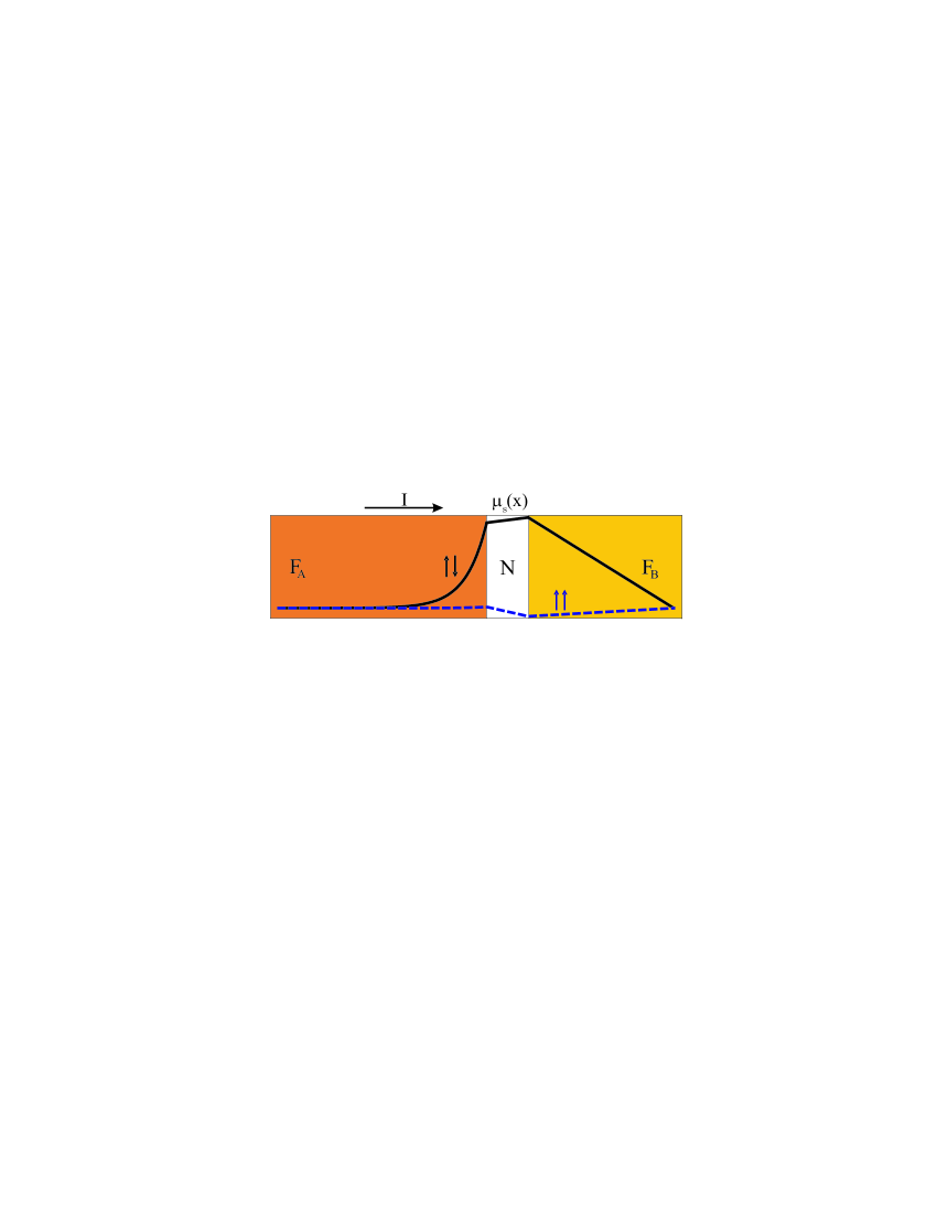
Figure 6: Illustration of the local charge and spin chemical potentials in a $\mathrm{F_{A}|N|F_{B}}$ spin valve biased by a voltage difference, for both parallel ($\uparrow\uparrow$) and anti-parallel ($\uparrow\downarrow$) alignments of the magnetizations. $\mathrm{F_{B}}(P=0.8,\lambda_{B}=0.1,S_{B}=-1\operatorname{\mu V}\mathrm{/}\mathrm{\operatorname{K}}$) has been chosen to have weak spin-flip scattering and thermopower compared with $\mathrm{F_{A}}(P=0.8,\lambda_{A}=10,S_{A}=-20\operatorname{\mu V}\mathrm{/}\mathrm{\operatorname{K}}$). The thin normal metal spacer is chosen to be highly conductive ($\rho_{N}\ll\rho_{A(B)}=10\operatorname{\mu\Omega}\mathrm{\operatorname{cm}}$) and to have a thermopower equal to that of $\mathrm{F_{B}}$. Note that spin accumulation is assumed to vanish at the two ends (at reservoirs).

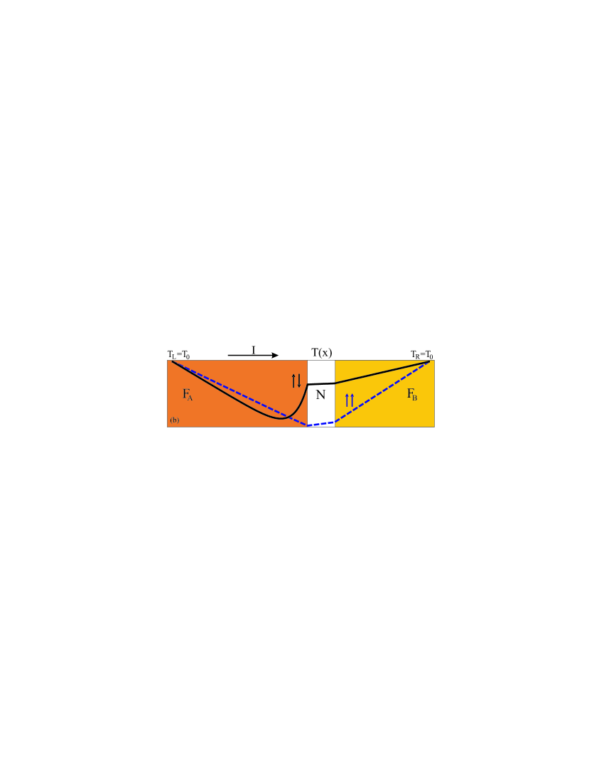
Figure 7: Illustration of local temperature distribution in the voltage biased $\mathrm{F_{A}|N|F_{B}}$ spin valve structure as in Fig. 6 for both parallel ($\uparrow\uparrow$) and anti-parallel ($\uparrow\downarrow$) alignments of the magnetizations. The different temperature profiles correspond to (a) $P^{\prime}\ll P$ ($P_{S}=-0.8$), (b) $P^{\prime}\gg P$ ($P_{S}=-1.8$). For the parallel alignment of the magnetizations the Peltier cooling is insensitive to spin-flips and reaches its maximum in the central node.

For the spin-valve structure in the presence of bulk spin-diffusion in the ferromagnets, we find the following results for the magnetoresistance MR as well as the magnetothermopower MTP. For the parallel configuration, as expected, no spin-flip contribution to the total resistance and thermopower is obtained i.e., $R_{P}=R_{A}+R_{B}$ and $S_{P}=(R_{A}S_{A}+R_{B}S_{B})/(R_{A}+R_{B})$. However, for the anti-parallel configuration we find

$$R_{AP}-R_{P}=\frac{\tanh\lambda}{\lambda}\frac{4P^{2}}{1-P^{2}}\frac{R_{A}R_{B}}{R_{A}+R_{B}},$$ (50)

$$S_{AP}-S_{P}=-\frac{\tanh\lambda}{\lambda}\frac{2PP_{S}}{1+PP_{S}}\frac{R_{A}R_{B}}{(R_{A}+R_{B})^{2}}(S_{A}+S_{B})$$ (51)

The MTP is therefore proportional to the giant magneto-resistance, independent of the spin-flip scattering strength $\lambda$. In contrast to the MR (at $\lambda\gg 1$) it is not possible to model spin-flip scattering for magneto-thermoelectric effects by replacing $R_{A(B)}$ by the resistance of the magnetically active region $\lambda^{-1}R_{A(B)}$.

VII Relevance for experiments

In the magnetic nanopillars considered by Fukushima et al.Fukushima et al. (2005a, b) the magnetic or normal leads that connect the central spacer to the wide external reservoirs are so long that the bulk scattering is important: A $100\;\mathrm{\operatorname{nm}}$ long cobalt wire has a resistance $\rho_{Co}L\simeq 6\;\mathrm{f}\operatorname{\Omega}\mathrm{\operatorname{m}}^{2}$ at room temperature, which is larger than the interface resistance $R_{Co|Cu}\approx 0.25\;\mathrm{f}\operatorname{\Omega}\mathrm{\operatorname{m}}^{2}$ (see Table. I). The effective thermopower $S_{L}\approx S_{Co}\simeq-31\operatorname{\mu V}\mathrm{/}\mathrm{\operatorname{K}}$ from the bulk scattering is also larger than the interface thermopower $S_{\mathrm{Co}|\mathrm{Cu}}\approx-6\operatorname{\mu V}\mathrm{/}\mathrm{\operatorname{K}}$. The interface contribution to the total thermopower would become more important for high-resistance interfaces, such as tunneling barriers or point contacts, or structures with thinner layers.

The lattice exchanges energy with the conduction electrons by inelastic electron-phonon interactions. In principle, there is a net heat current flowing between the electron system and the lattice/substrate. In a steady state situation it is reasonable to assume that electron and lattice temperatures are identical and resistance changes reflect the electron temperature. When Peltier cooling and Joule electron heating compensate each other the temperature change vanishes. Estimating the nonlinear electron heating in the island by $\mathcal{L}_{0}T\Delta T_{N}=G_{tot}^{-1}I^{2}/2(G_{L}+G_{R})$ and using Eq. (30) in terms of the lumped conductances and thermopowers, the compensation current $I_{p}$ or cooling-power $R_{0}I_{p}$ for $\mathrm{F}_{A}$$|$$\mathrm{N}$$|$$\mathrm{N}_{B}$ structures such as Co$|$Cu$|$Au nanopillars can be expressed as

$$R_{0}I_{p}\approx 2(\gamma_{L}\Pi_{L}-\Pi_{R}).$$ (52)

Such an expression holds as well for $\text{Co}|\text{Cu}|\text{Co}|\text{Au structures}$ when the magneto-Peltier effect for the symmetric part $\text{Co}|\text{Cu}|\text{Co}$ can be disregarded.Fukushima et al. (2005a, b) The factor of $2$ difference with Refs. Fukushima et al., 2005a, b has been noted already above. We find below that including this factor leads to a better agreement of a simple model of bulk thermopowers with experiments. Also the too large pillar cross sections with which Gravier et al.Gravier et al. (2006c) fitted their numerical results to the experiments can be traced back to this factor 2 in the Joule heating. Our model might not be appropriate for Fukushima’s samples that contain a highly resistant, presumably oxide, layer over which much of the voltage drop occurs. Such a layer, when sufficiently thick, might be better described as a bulk resistor in which Joule heat is preferentially generated. At the compensation current $I_{p},$ finite temperature variation profiles may persist since the Joule and Peltier sources are spatially separated. A simulation beyond our simple model might then be required for a quantitative description.

Experimental values of $R_{0}I_{p}$ for $\text{Co}|\text{Au}$ nanopillars can be read off the figures published by different groups, amounting to (in $\operatorname{mV}$) 19 (Ref. Albert et al., 2000), 23.0 (Ref. Koch et al., 2004), 22.5 (Ref. Fukushima et al., 2005a, b). These numbers agree well with the following results. For a finite length of the bulk layers, i.e. $L_{Co}=60\;\operatorname{nm}$ and $L_{Au}=120\;\operatorname{nm}$ and taking into account the interface scattering, when disregarding the spin polarization of the thermopower $P_{S}$ we find $R_{0}I_{p}=19.5\;\operatorname{mV}.$ Here we also assumed $G_{R}\ll G_{L}$ caused by an oxide layer on the non-magnetic side of the structure, $S_{\mathrm{Cu|Au}}\simeq 0$, $S_{\mathrm{Co|Cu}}\simeq-6\;\operatorname{\mu V}\mathrm{/}\mathrm{\operatorname{K}}$ and used the bulk parameters from Ref. Gravier et al., 2006c. $R_{0}I_{p}\approx 2(\Pi_{Co}-\Pi_{Au})=19.6\;\operatorname{mV}$ indicates that the Peltier cooling is not significantly affected by interface scattering. A finite $P_{S}$ can enlarge or reduce the above estimates. The spin-entropy coupling factor $\gamma_{L}\approx(1-P^{\prime}P)/(1-P^{2})$ when the bulk and interface spin polarizations are the same. For Co we took $P=0.44$ (Ref. Soulen Jr. et al., 1998). Conflicting values $P_{S}=-0.18<0$ ($S^{\uparrow}=0.7S_{\downarrow}$) (Ref. Gravier et al., 2006a, b) and $P_{S}=+0.42>0$ ($S^{\uparrow}=-30\operatorname{\mu V}\mathrm{/}\mathrm{\operatorname{K}},S_{\downarrow}=-12\operatorname{\mu V}\mathrm{/}\mathrm{\operatorname{K}}$) (Ref. Cadeville and Roussel, 1971) are found in the literature. According to Table I, $P_{S}$ of the $\text{Co}|\text{Cu}$ interface can also have either sign. The two values for $P_{S}$ modify the above estimate to $R_{0}I_{p}=21$ and $17\operatorname{mV}$, respectively, possibly favoring a $P_{S}<0$ when comparing with the observed values.

The adiabatic spin-entropy expansion term $(k_{B}T\ln 2)I/e$ considered in Ref. Katayama-Yoshida et al., 2007 is in our opinion an extrapolation of a concept from equilibrium thermodynamics that does not play a role in the current induced (non-equilibrium) Peltier cooling.

We proceed by estimating the magnitude of the temperature drop that can be realized by the Peltier effect in the magnetic heterostructure $\mathrm{Co}\left(60\operatorname{nm}\right)|\mathrm{Au}\left(20\operatorname{nm}\right)|\mathrm{Cr}\left(120\operatorname{nm}\right)$.Gravier et al. (2006c) At room temperature the bulk thermopowers of both Co and Cr are relatively large and have opposite signs ($S_{\mathrm{Cr}}=+21.56\operatorname{\mu V}\mathrm{/}\mathrm{\operatorname{K}}$). The temperature drop $\Delta T_{\mathrm{Au}}\approx I_{p}\left(S_{L}-S_{R}\right)/\left(\mathcal{L}_{0}\left(G_{L}+G_{R}\right)\right)$ in the central island amounts to $4.8\operatorname{K}$ at $I_{p}=10\mathrm{\operatorname{mA}}$ for a cross-section of $70\operatorname{nm}\times 200\operatorname{nm}$, at a current density of $\sim 10^{8}\mathrm{\operatorname{A}/\operatorname{cm}}^{2}$, which is close to the maximum temperature drop in the temperature profiles computed in Ref. Gravier et al., 2006c (we find a cooling-power $R_{0}I_{p}=30\operatorname{mV},$ which is smaller than the observed value $41\operatorname{mV},$ however). The temperature reduction per unit of electric current is sensitive to the thickness of the leads. For the thick magnetic layers $\Delta T_{\mathrm{Au}}\approx I_{p}(S_{\mathrm{Co}}-S_{\mathrm{Cr}})/\mathcal{L}_{0}(G_{\mathrm{Co}}+G_{\mathrm{Cr}})$. Spin polarization of the thermopower in Co can modify the amount of the temperature reduction, up to $8\%$ for $|P_{S}|=0.4$.

In Fukushima’s experiments the leads connected to the external reservoirs are long compared to the spin-flip diffusion length. In that regime a magneto-Peltier effect should be small. Let us therefore consider a spin-valve structure such as $\mathrm{Co}_{001}\left(10\operatorname{nm}\right)|\mathrm{Au}\left(20\operatorname{nm}\right)|\mathrm{Co}_{001}\left(5\operatorname{nm}\right),$ in which spin-flip scattering is less important. Due to the different lengths of the bulk Co layers the Peltier cooling does not vanish at this structure even for a parallel magnetic configuration; recall for example Eq. (41) when $G_{1}\neq G_{2}$. For the parallel alignment of the magnetizations with $P_{A}=P_{B}$ one finds $\gamma_{L(R)}^{MP}=1,$ equivalent to a normal metal structure, whereas the spin-entropy coupling parameter differs for the anti-parallel magnetic configuration when $P_{A}=-P_{B}$. Let us now consider a small $G_{1}=0.01G_{2}$ e.g. caused by an oxide layer at the junction between the thick Co layer and the normal metal spacer, using data in Table I for the interface scattering (at room temperature), and adopting bulk values $P_{S}=-1.18$ and $P_{S}=0.42,$ we find respectively the magneto-Peltier signals $R_{0}[I_{p}(\pi)-I_{p}(0)]=-1.59$ and $+6.7\operatorname{mV}$, which should be experimentally observable. Replacing the bulk parameters of the thicker Co layer by $\rho_{Fe}=9.7\times 10^{-8}\operatorname{\Omega}\mathrm{\operatorname{m}}$ and $S_{Fe}=+20\operatorname{\mu V}\mathrm{/}\mathrm{\operatorname{K}}$, the Peltier cooling is increased and the magneto-Peltier signals read $R_{0}[I_{p}(\pi)-I_{p}(0)]=+3.2$ and $-2\operatorname{mV}$. Finally we mention that the magneto-Peltier cooling via the bulk scattering can be also sensitive to the degree of energy relaxation, but discussion of the details is beyond the scope of the present paper.

Since the thermopower-to-conductance ratios $S_{i}/G_{i}$ of the intermetallic interfaces studied up to now are smaller than the bulk values for thicker magnetic layers, for the material combinations considered above we do not expect an increased cooling power by reducing the thickness of the nanopillars to the interface-dominated regime. The interface contributions are important for (classical) point contacts or pinholes in thick tunneling barriers, since $S_{I}$ can remain unmodified while $G_{I}$ is strongly reduced. Magnetic tunnel junctions are interesting subjects for magneto-Peltier studies since much higher $S/G$ ratios can be expected.

The spin Seebeck effect Uchida et al. (2008) recently observed in a very long ferromagnetic metal appears to have a different origin than the conventional mechanisms of spin and heat diffusion. The observed thermoelectric spin signal parametrized by a spin-Seebeck coefficient ($S_{s}=-2\operatorname{nV}/\operatorname{K}$ at room temperature Uchida et al. (2008)) is much smaller than both the interface and bulk thermopowers considered above. We therefore do not expect that the spin Seebeck effect would significantly modify our findings.

VIII Summary and conclusions

We studied the Peltier effect in nanoscale metallic multilayer structures involving ferromagnets using a newly developed semiclassical theory of thermoelectric transport in magnetic heterostructures including spin relaxations and the effects of electron interactions in limiting cases. The Peltier cooling/heating depends in general on the spin-degree of freedom as a function of spin and energy-dependent bulk and interface scattering. We predict a magneto-Peltier effect in spin valves, i.e. a dependence of Peltier cooling on the relative alignment of the two magnetization directions, that can arise from the spin-polarization of thermopowers and is sensitive to the spin-flip scattering as well as strength of the inelastic collisions in the normal metal spacer. Similar behavior is found for the magneto-thermopower which might be even easier to observe in experiments (when thermoelectric voltage is measured rather than temperature). For ferromagnetic layers with thickness of the order or smaller than the spin-flip diffusion length the magneto-Peltier effect should be observable in terms of magnetic-field-dependent resistance shifts in the $R(I)$ characteristics i.e. the cooling-power. Estimates for the Peltier cooling based on our model and available parameters agree relatively well with experiments as well as numerical models in which the bulk scattering dominates.

Appendix A Phonons

The Peltier effect in the presence of phonon heat conduction and electron-phonon interactions can be modeled in linear response as follows: The net heat current flowing between the electron and phonon subsystems of the island for small temperature differences $T_{e}^{N}-T_{p}^{N}\ll T_{p}^{N}$ may be parametrized by the simple linear equation $\dot{Q}_{e-p}=-\kappa_{e-p}(T_{e}^{N}-T_{p}^{N})$. Groeneveld et al. (1995) For a phonon temperature drop of $\Delta T_{p}$ across an interface, $\dot{Q}_{p}=-\kappa_{p}\Delta T_{p}$ with $\kappa_{p}$ the phonon thermal conductance of the junction. Gundrum et al. (2005) The energy conservation laws then read: $\dot{Q}_{e1}+\dot{Q}_{e2}+\dot{Q}_{e-p}=0$ and $\dot{Q}_{p1}+\dot{Q}_{p2}-\dot{Q}_{e-p}=0$ for the electron and phonon subsystems, respectively. The electron temperature in the node, Eq. (5), is then modified as follows

$$\Delta T_{e}^{N}=\frac{(\Pi_{1}-\Pi_{2})I}{\kappa_{e1}+\kappa_{e2}+\gamma_{p}(\kappa_{p1}+\kappa_{p2})}$$ (53)

and $\Delta T_{p}^{N}=\gamma_{p}\Delta T_{e}^{N}$ where $\gamma_{p}=\kappa_{e-p}/(\kappa_{p1}+\kappa_{p2}+\kappa_{e-p})$. In the limit $\kappa_{p1(2)}\ll\kappa_{e-p}$ the Peltier cooling is reduced by the sum of the total thermal conductances $\kappa_{1(2)}=\kappa_{e1(2)}+\kappa_{p1(2)}$. The figure of merit $S\Delta T_{e}^{N}/\Delta V$ is then further decreased by taking into account the contribution of the phonon heat conduction ($\dot{Q}_{p}\neq 0$).

Appendix B Thermoelectric spin diffusion equations

In a diffusive magnetic metal in the steady state the Boltzmann transport equation in the relaxation time approximation leads to the following spectral spin diffusion equations for the local variation of the spin distribution functions $f^{\uparrow(\downarrow)}(\epsilon)$ for each spin $\alpha$ as

$$\nabla^{2}f^{\alpha}(\epsilon)=\frac{f^{\alpha}(\epsilon)-f^{-\alpha}(\epsilon)}{(l_{sf}^{\alpha})^{2}},$$ (54)

where $l_{sf}^{\alpha}=\sqrt{D^{\alpha}\tau_{sf}^{\alpha}}$ are the spin-dependent diffusion lengths. Under the detailed balance condition $\mathcal{N}^{\uparrow}/\tau_{sf}^{\uparrow}=\mathcal{N}^{\downarrow}/\tau_{sf}^{\downarrow}$ the spectral spin diffusion equations can be rewritten as

$$\nabla^{2}f_{s}(\epsilon)=\frac{f_{s}(\epsilon)}{l_{sf}^{2}},$$ (55)

$$\nabla^{2}f_{c}(\epsilon)=-P\frac{f_{s}(\epsilon)}{2l_{sf}^{2}}.$$ (56)

where $(l_{sf})^{-2}=(l_{sf}^{\uparrow})^{-2}+(l_{sf}^{\downarrow})^{-2}$ and the charge and spin distribution functions, $f_{c(s)}=\left(f^{\uparrow}\pm f^{\downarrow}\right)/2,$ have been introduced. In the strongly thermalized regime the spin diffusion equations can be expressed in terms of the spin chemical potentials $\mu_{\uparrow(\downarrow)}=(\mu_{c}\pm\mu_{s}/2)$ and the electron temperature $T$. After inserting the linear expansions

$$f_{s}(\epsilon)\approx\left(-\frac{\partial f_{0}}{\partial\epsilon}\right)\mu_{s},$$ (57)

$$\nabla^{2}f_{c(s)}(\epsilon)\approx\left(-\frac{\partial f_{0}}{\partial\epsilon}\right)\left(\nabla^{2}\mu_{c(s)}+\frac{\epsilon-\mu}{T}\nabla^{2}T\right),$$ (58)

into the above diffusion equations we can integrate over energies by using the Sommerfeld approximation (see Eq. (3)). We assume $S^{2}\ll\mathcal{L}_{0}$ and disregard an energy dependence of the spin diffusion length $l_{sf}$ (which is allowed when $2PS_{sf}\ll(P^{\prime}-P)S$ in which $S_{sf}=-eL_{0}T\partial_{\epsilon}lnl_{sf}(\epsilon)|_{\epsilon_{F}}$), but keep the energy dependence of the spin polarization $P$, recall Eq. (29). One then arrives at the thermoelectric spin diffusion equations expressed in Eqs. (46-48). Among the spin diffusion equations Eqs. (46) and (47) are already well known.Valet and Fert (1993) Eq. (48) represents a spin-heat coupling for the electron spin diffusion in the presence of spin polarization of thermopower.

References

- Giazotto et al. (2006) F. Giazotto, T. T. Heikkilä, A. Luukanen, A. M. Savin, and J. P. Pekola, Rev. Mod. Phys. 78, 217 (2006).
- Hicks and Dresselhaus (1993) L. D. Hicks and M. S. Dresselhaus, Phys. Rev. B 47, 12727 (1993).
- Sales (2002) B. C. Sales, Science 295, 1248 (2002).
- Boukai et al. (2008) A. I. Boukai, Y. Bunimovich, J. Tahir-Kheli, J.-K. Yu, W. A. Goddard, and J. R. Heath, Nature 451, 168 (2008).
- Hochbaum et al. (2008) A. I. Hochbaum, R. Chen, R. D. Delgado, W. Liang, E. C. Garnett, M. Najarian, A. Majumdar, and P. Yang, Nature 451, 163 (2008).
- Venkatasubramanian et al. (2001) R. Venkatasubramanian, E. Siivola, T. Colpitts, and B. O’Quinn, Nature 413, 597 (2001).
- Ohta et al. (2007) H. Ohta, S. Kim, Y. Mune, T. Mizoguchi, K. Nomura, S. Ohta, T. Nomura, Y. Nakanishi, Y. Ikuhara, M. Hirano, et al., Nature Materials 6, 129 (2007).
- Molenkamp et al. (1992) L. W. Molenkamp, T. Gravier, H. van Houten, O. J. A. Buijk, M. A. A. Mabesoone, and C. T. Foxon, Phys. Rev. Lett. 68, 3765 (1992).
- van Houten et al. (1992) H. van Houten, L. W. Molenkamp, C. W. J. Beenakker, and C. T. Foxon, Semiconductor Science and Technology 7, B215 (1992).
- Johnson and Silsbee (1987) M. Johnson and R. H. Silsbee, Phys. Rev. B 35, 4959 (1987).
- Johnson (2003) M. Johnson, J. of Superconductivity 16, 679 (2003).
- Wegrowe (2000) J.-E. Wegrowe, Phys. Rev. B 62, 1067 (2000).
- Gravier et al. (2006a) L. Gravier, S. Serrano-Guisan, F. Reuse, and J.-P. Ansermet, Phys. Rev. B 73, 024419 (2006a).
- Gravier et al. (2006b) L. Gravier, S. Serrano-Guisan, F. Reuse, and J.-P. Ansermet, Phys. Rev. B 73, 052410 (2006b).
- Serrano-Guisan et al. (2006) S. Serrano-Guisan, G. di Domenicantonio, M. Abid, J. P. Abid, M. Hillenkamp, L. Gravier, J.-P. Ansermet, and C. Félix, Nature Materials 5, 730 (2006).
- Tsyplyatyev et al. (2006) O. Tsyplyatyev, O. Kashuba, and V. I. Fal’ko, Phys. Rev. B 74, 132403 (2006).
- Hatami et al. (2007) M. Hatami, G. E. W. Bauer, Q. F. Zhang, and P. J. Kelly, Phys. Rev. Lett. 99, 066603 (2007).
- Fukushima et al. (2005a) A. Fukushima, K. Yagami, A. A. Tulapurkar, Y. Suzuki, H. Kubota, A. Yamamoto, and S. Yuasa, Jpn. J. Appl. Phys. 44, L12 (2005a).
- Fukushima et al. (2005b) A. Fukushima, H. Kubota, A. Yamamoto, Y. Suzuki, and S. Yuasa, IEEE Trans. Mag. 41, 2571 (2005b).
- Gravier et al. (2006c) L. Gravier, A. Fukushima, H. Kubota, A. Yamamoto, and S. Yuasa, J. Phys. D: Appl. Phys. 39, 5267 (2006c).
- Katayama-Yoshida et al. (2007) H. Katayama-Yoshida, T. Fukushima, V. A. Dinh, and K. Sato, Jpn. J. Appl. Phys. 46, L777 (2007).
- Dubi and Ventra (2008) Y. Dubi and M. Di Ventra, Phys. Rev. B. 79, 081302(R) (2009).
- Brataas et al. (2000) A. Brataas, Y. V. Nazarov, and G. E. W. Bauer, Phys. Rev. Lett. 84, 2481 (2000).
- Brataas et al. (2001) A. Brataas, Y. V. Nazarov, and G. E. W. Bauer, Eur. Phys. J. B 22, 99 (2001).
- Brataas et al. (2006) A. Brataas, G. E. W. Bauer, and P. J. Kelly, Phys. Rep. 427, 157 (2006).
- Valet and Fert (1993) T. Valet and A. Fert, Phys. Rev. B 48, 7099 (1993).
- Bass and Pratt Jr. (1999) J. Bass and W. P. Pratt Jr., J. Magn. & Magn. Mater. 200, 274 (1999).
- MacDonald (1962) D. K. C. MacDonald, Thermoelectricity: An Introduction to the Principles (John Wiley & Sons, New York, United States of America, 1962).
- Xia et al. (2006) K. Xia, M. Zwierzycki, M. Talanana, P. J. Kelly, and G. E. W. Bauer, Phys. Rev. B 73, 064420 (2006).
- Zhang et al. (Unpublished) Q. F. Zhang, P. J. Kelly, M. Hatami, and G. E. W. Bauer (Unpublished).
- Schep et al. (1997) K. M. Schep, J. B. A. N. van Hoof, P. J. Kelly, G. E. W. Bauer, and J. E. Inglesfield, Phys. Rev. B 56, 10805 (1997).
- Ashcroft and Mermin (1976) N. W. Ashcroft and N. D. Mermin, Solid State Physics (Holt-Saunders International Editions, Philadelphia, 1976).
- Colquitt, Jr. et al. (1971) L. Colquitt, Jr., H. R. Fankhauser, and F. J. Blatt, Phys. Rev. B 4, 292 (1971).
- Gundrum et al. (2005) B. C. Gundrum, D. G. Cahill, and R. S. Averback, Phys. Rev. B 72, 245426 (2005).
- Guttman et al. (1995) G. D. Guttman, E. Ben-Jacob, and D. J. Bergman, Phys. Rev. B 52, 5256 (1995).
- Nagaev (1995) K. E. Nagaev, Phys. Rev. B 52, 4740 (1995).
- Pothier et al. (1997) H. Pothier, S. Guéron, N. O. Birge, D. Esteve, and M. H. Devoret, Phys. Rev. Lett. 79, 3490 (1997).
- Cadeville and Roussel (1971) M. C. Cadeville and J. Roussel, J. Phys. F: Met. Phys. 1, 686 (1971).
- Piraux et al. (1992) L. Piraux, A. Fert, P. A. Schroeder, R. Loloee, and P. Etienne, J. Magn. & Magn. Mater. 110, L247 (1992).
- Shi et al. (1996) J. Shi, K. Pettit, E. Kita, S. S. P. Parkin, R. Nakatani, and M. B. Salamon, Phys. Rev. B 54, 15273 (1996).
- Gravier et al. (2004) L. Gravier, A. Fábián, A. Rudolf, A. Cachin, J.-E. Wegrowe, and J.-P. Ansermet, J. Magn. & Magn. Mater. 271, 153 (2004).
- Hatami et al. (Unpublished) M. Hatami, T. Heikkil, and G. E. W. Bauer (Unpublished).
- Zwierzycki et al. (2005) M. Zwierzycki, Y. Tserkovnyak, P. J. Kelly, A. Brataas, and G. E. W. Bauer, Phys. Rev. B 71, 064420 (2005).
- S. Urazhdin and Pratt, Jr. (2005) S. Urazhdin, R. Loloee and W. P. Pratt, Jr., Phys. Rev. B 71, 100401(R) (2005).
- Kovalev et al. (2006) A. A. Kovalev, G. E. W. Bauer, and A. Brataas, Phys. Rev. B 73, 054407 (2006).
- Zwierzycki et al. (2008) M. Zwierzycki, P. A. Khomyakov, A. A. Starikov, K. Xia, M. Talanana, P. X. Xu, V. M. Karpan, I. Marushchenko, I. Turek, G. E. W. Bauer, et al., phys. stat. sol. B 245, 623 (2008).
- Turek et al. (1997) I. Turek, V. Drchal, J. Kudrnovský, M. Šob, and P. Weinberger, Electronic Structure of Disordered Alloys, Surfaces and Interfaces (Kluwer, Boston-London-Dordrecht, 1997).
- Andersen and Jepsen (1984) O. K. Andersen and O. Jepsen, Phys. Rev. Lett. 53, 2571 (1984).
- Andersen et al. (1986) O. K. Andersen, Z. Pawlowska, and O. Jepsen, Phys. Rev. B 34, 5253 (1986).
- Ando (1991) T. Ando, Phys. Rev. B 44, 8017 (1991).
- Xia et al. (2001) K. Xia, P. J. Kelly, G. E. W. Bauer, I. Turek, J. Kudrnovský, and V. Drchal, Phys. Rev. B 63, 064407 (2001).
- Soven (1967) P. Soven, Phys. Rev. 156, 809 (1967).
- Xia et al. (2002) K. Xia, P. J. Kelly, G. E. W. Bauer, A. Brataas, and I. Turek, Phys. Rev. B 65, 220401(R) (2002).
- R. J. Gripshover, J. B. VanZytveld, and J. Bass (1967) R. J. Gripshover, J. B. VanZytveld and J. Bass, Phys. Rev. 163, 598 (1967).
- Bass (1982) J. Bass, Thermoelectricity: in AccessScience@McGraw-Hill (New York, 2000).
- Jonson and Mahan (1980) M. Jonson and G. D. Mahan, Phys. Rev. B 21, 4223 (1980).
- Kontani (2003) H. Kontani, Phys. Rev. B 67, 014408 (2003).
- F. J. Blatt and Schroeder (1967) V. R. F. J. Blatt, D. J. Flood and P. A. Schroeder, Phys. Rev. Lett. 18, 395 (1967).
- Blatt (1976) F. J. Blatt, Thermoelectric Power of Metals (New York : Plenum Press, New York, United States of America, 1976).
- Gurevich and Logvinov (2005) Y. G. Gurevich and G. N. Logvinov, Semiconductor Science and Technology 20, R57 (2005).
- Kovalev et al. (2002) A. A. Kovalev, A. Brataas, and G. E. W. Bauer, Phys. Rev. B 66, 224424 (2002).
- Albert et al. (2000) F. J. Albert, J. A. Katine, R. A. Buhrman, and D. C. Ralph, Appl. Phys. Lett. 77, 3809 (2000).
- Koch et al. (2004) R. H. Koch, J. A. Katine, and J. Z. Sun, Phys. Rev. Lett. 92, 088302 (2004).
- Soulen Jr. et al. (1998) R. J. Soulen Jr., J. M. Byers, M. S. Osofsky, B. Nadgorny, T. Ambrose, S. F. Cheng, P. R. Broussard, C. T. Tanaka, J. Nowak, J. S. Moodera, et al., Science 282, 85 (1998).
- Uchida et al. (2008) K. Uchida, S. Takahashi, K. Harii, J. Ieda, W. Koshibae, K. Ando, S. Maekawa, and E. Saitoh, Nature 455, 778 (2008).
- Groeneveld et al. (1995) R. H. M. Groeneveld, R. Sprik, and A. Lagendijk, Phys. Rev. B 51, 11433 (1995).