X-ray and Radio Timing of the Pulsar in 3C 58

Abstract

We present timing data spanning 6.4 yr for the young and energetic PSR J0205+6449, in the supernova remnant 3C 58. Data were obtained with the Rossi X-ray Timing Explorer, the Jodrell Bank Observatory and the Green Bank Telescope. We present phase-coherent timing analyses showing timing noise and two spin-up glitches with fractional frequency increases of $\sim 3.4\times 10^{-7}$ near MJD 52555, and $\sim 3.8\times 10^{-6}$ between MJDs 52777 and 53062. These glitches are unusually large if the pulsar was created in the historical supernova in 1181 as has been suggested. For the X-ray timing we developed a new unbinned maximum-likelihood method for determining pulse arrival times which performs significantly better than the traditional binned techniques. In addition, we present an X-ray pulse profile analysis of four years of RXTE data showing that the pulsar is detected up to $\sim$40 keV. We also present the first measurement of the phase offset between the radio and X-ray pulse for this source, showing that the radio pulse leads the X-ray pulse by $\phi=0.10\pm 0.01$ in phase. We compile all known measurements of the phase offsets between radio and X-ray and radio and $\gamma$-ray pulses for X-ray and $\gamma$-ray pulsars. We show that there is no relationship between pulse period and phase offset, supported by our measurement of the phase offset for PSR J0205+6449.

1 INTRODUCTION

PSR J0205+6449 is a 65-ms rotation-powered pulsar residing in the center of the supernova remant 3C 58. The pulsar was discovered in a 2002 Chandra X-ray Observatory (CXO) observation of the source (Murray et al., 2002) and subsequently detected as a radio pulsar (Camilo et al., 2002). It is one of the most energetic pulsars in the Galaxy, with a spin-down luminosity of $\dot{E}\sim 2.7\times 10^{37}$erg s^-1.

The possible association between the 3C 58 pulsar/pulsar wind nebula complex and the historical supernova SN 1181 has been a matter of debate. 3C 58 is the only known source positionally coincident and energetically compatible with the historical supernova, strongly suggesting an association (Stephenson & Green, 2002). However, in recent years, evidence has been mounting that the association may be spurious and that the true age of the pulsar may be closer to its characteristic age, $\tau_{c}\equiv\nu/2\dot{\nu}=5.4$ kyr (where $\nu$ is the pulsar’s rotation frequency and $\dot{\nu}$ its derivative), rather than the implied historic age of 828 yr. If the source is 828 yr-old, the size of the remnant implies a large expansion velocity that is hard to reconcile with the measured velocities of the optical filaments (Fesen, 1983) and the expansion speed of the synchrotron bubble (Bietenholz et al., 2001; Bietenholz, 2006). The characteristic age estimate assumes that the pulsar was born spinning rapidly ($\nu_{0}\gg\nu$) and that the temporal spin evolution of the pulsar has proceeded according to a simple magnetic dipole spin-down model. These assumptions are known to fail in some cases, such as for PSR J1811$-$1925 in the supernova remnant G11.2$-$0.3, for which the pulsar’s characteristic age appears to be a factor of $\sim$15 greater than that of the remnant (e.g. Torii et al., 1999; Kaspi et al., 2001; Tam & Roberts, 2003). The two ages can be reconciled if PSR J1811$-$1925 was born spinning slowly, with $\nu_{0}\simeq\nu$. Similarly, the pulsar J0538+2817 has a characteristic age of 620 kyr, but a well established kinematic age of $\sim$40 kyr, implying a long initial spin period of $\sim$138 ms (Kramer et al., 2003; Ng et al., 2007). Likewise, if PSR J0205+6449 was born spinning with a period of $\sim$60 ms, the estimated age of the pulsar could be reconciled with the historical supernova age (Murray et al., 2002). An alternate explanation of the age disparity for PSR J0205+6449 is if the pulsar were born with a short spin period but evolved more rapidly than is typically assumed for magnetic dipole braking.

In principle, it may be possible to to gain information about a pulsar’s true age via its glitching behavior. Pulsars in general, and young pulsars in particular, exhibit two types of rotational irregularities superposed on their secular spin down. Glitches are characterized by a sudden increase in $\nu$, sometimes followed by an exponential decay, and are often accompanied by an increase in the magnitude of $\dot{\nu}$. Glitches are common in young pulsars, particularly in pulsars aged $\sim$10-100 kyr, and provide valuable information about the superfluid interiors of pulsars. The fractional sizes of detected glitches span 5 orders of magnitude, with $\Delta{\nu}/{\nu}\sim 10^{-10}-10^{-5}$ (Janssen & Stappers, 2006; Hobbs et al., 2002). The nature of glitches appears to change with age. Glitches in the youngest Crab-like pulsars (1-2 kyr) tend to be small in magnitude, $\Delta{\nu}/{\nu}\sim 10^{-9}-10^{-8}$, and if the frequency recovers, it tends to recover almost completely. By contrast, glitches in older Vela-like pulsars are typically larger, with magnitudes of $\Delta{\nu}/{\nu}\sim 10^{-7}-10^{-6}$, and typically recover only a small percentage of the frequency change (Lyne et al., 2000).

Young pulsars are also prone to large stochastic variations in their spin-down rates, known as timing noise. These noise processes are observed as long-term trends in timing residuals after the removal of deterministic spin-down effects. Timing noise tends to be the most severe in young pulsars and a correlation with $\dot{\nu}$ is well established (Cordes & Downs, 1985; Arzoumanian et al., 1994; Urama et al., 2006). The low-frequency and broad-band nature of timing noise leads to difficulties in its analysis. Moreover, the physical causes of timing noise are poorly understood. It could be that fluctuations in the superfluid interiors of neutron stars cause a torque on the pulsar (Cordes & Greenstein, 1981), or that interactions between the pulsar and the magnetosphere impart a torque (Cheng, 1987), to name two possibilities.

In this paper, we present three coherent timing solutions for PSR J0205+6449 spanning 6.4 yr with data obtained from the Green Bank Telescope (GBT), the Jodrell Bank Observatory (JBO) and the Rossi X-ray Timing Explorer (RXTE). We discuss two large glitches and timing noise found in these data. We also present an analysis of the high energy emission of the pulsar from the RXTE data by examining the X-ray pulse profile from 2 – 40 keV and the phase offset between the radio and X-ray pulses.

2 OBSERVATIONS AND ANALYSIS

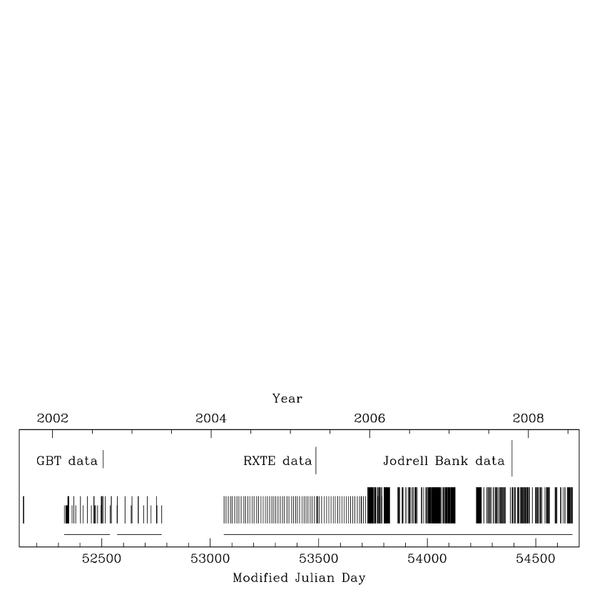
Figure 1: Distribution of observations of PSR J0205+6449 from RXTE, GBT, and JBO over 6.9 yr. GBT data are indicated with short lines, RXTE data with medium length lines, and JBO data with long lines. The three coherent timing solutions, spanning a total of 6.4 yr, are indicated with horizontal lines along the bottom of the plot.

X-ray observations were taken with RXTE; radio observations were taken with the GBT and JBO, as detailed below. The data were unevenly spaced throughout 6.9 yr, as shown in Figure 1, and include a 202-day gap (between observations taken in RXTE Cycle 6 and Cycle 7) and a 287-day gap (corresponding to Cycle 8). GBT data are shown with short lines, RXTE data are shown with medium-length lines, and JBO data are shown with long lines. The first set of observations from RXTE Cycle 6 are only considered for the pulse profile analysis (§4) and are not included in the 6.4 yr of data for our timing analysis (§3.1).

2.1 RXTE Observations and Analysis

Observations of PSR J0205+6449 were made using the Proportional Counter Array (PCA; Jahoda et al., 2006) on board RXTE. The PCA is an array of five collimated Xenon/methane multi-anode proportional counter units (PCUs) operating in the 2 – 60 keV range, with a total effective area of approximately $\rm{6500~{}cm^{2}}$ and a field of view of $\rm{\sim 1^{o}}$ FWHM.

Data were obtained during RXTE observing Cycles 7, 9, and 10, spanning a period of 4 yr from MJD 52327 to 53813, with a long gap (from MJD 52752 to 53036) corresponding to RXTE observing Cycle 8. In addition, four observations were taken in observing Cycle 6 (17.1 hr exposure over MJD 52138 – 52141). Because of the long data gap between the Cycle 6 data and the subsequent observations in Cycle 7 (202 days), they could not be unambiguously phase connected, rendering these observations of limited interest for our timing analysis. They were considered for a pulse profile analysis discussed in §4. The frequency for each Cycle 6 observation was determined by a periodogram analysis, which was then used for folding the data. All of the RXTE data were collected in “GoodXenon” mode, which records the arrival time (with 1-$\mu$s resolution) and energy (256 channel resolution) of every unrejected event. Typically, 3 PCUs were operational during an observation. For our timing analysis, we used only the first layer of each operational PCU in the energy range 2 – 18 keV, as this maximizes the signal-to-noise ratio of individual observations for this source.

Observations were downloaded from the HEASARC archive and photon arrival times were converted to barycentric dynamical time (TDB) at the solar system barycenter using the J2000 source position determined using data from CXO, RA = $02^{\rm{h}}$ $05^{\rm{m}}$ $37\fs 92\pm 0\fs 02$, Dec $=64^{\circ}$ $49\arcmin$ $42.8\arcsec\pm 0.72\arcsec$ (Slane et al., 2002) and the JPL DE200 solar system ephemeris with the FITS tool ‘faxbary’.

We noted that two observations directly following the leap second occurring on 2006 January 1 had incorrect clock corrections, confirmed by the RXTE team (C. Markwardt, private communication). This was fixed by adding a 1 s time jump to each pulse time-of-arrival obtained from these observations.

2.1.1 A New X-ray Timing Technique

The X-ray pulse profile as measured in each observing session by RXTE has two narrow components separated by approximately one-half of a rotation of the pulsar (See Fig. 2). Such sharp pulse features are usually very helpful for timing analyses, however, the “signal-to-noise” ratio (here defined as the ratio of pulsed source counts to all other counts) for the RXTE observations was very low, with typical values near 6$\times$10^-3. These levels are so low that for some observations the pulses were not easily visible in the binned pulse profile plots. Therefore, in order to determine the pulse times-of-arrival (TOAs) from the X-ray data, we used a new and simple maximum-likelihood (ML) technique. This method avoids the information loss inherent in binning event-based (i.e. photon) pulse profiles. The inputs to the method are an accurate model pulse profile $I(\Phi)$ of intensity, including both signal and the average noise level or background, as a function of rotational phase $\Phi$ (where $0\leq\Phi<1$), and the computed rotational phases $\phi_{i}$ of the $N$ events (where $1\leq i\leq N$) from the observation according to the best timing model of the pulsar. We normalize $I(\Phi)$ so that it has unit area and can be treated as a probability density function for the individual event arrival times.

If we assume an arrival offset $t/P$ (where $P$ is the spin period) of rotational phase (where $0\leq t/P<1$), we can compute a probability or likelihood that our data has that offset from the template using ${\rm{Prob}}(t/P)=\prod_{i=1}^{N}I(\phi_{i}-t/P)$. If we compute a large grid of 1000-10000 evenly-spaced probabilities for offsets $t/P$ between 0 and 1, the resulting distribution describes the probability density for the average pulse arrival time. When normalized, we can determine the most likely arrival time, or by suitably integrating the distribution, the median arrival time and error estimates for the arrival time.

To test how well the ML technique determines TOAs compared to the traditional binned Fourier-based methods typically used in radio pulsar timing (Taylor, 1992), we simulated $\sim$100,000 high-energy observations of pulsars with both a pulse profile like that of PSR J0205+6449 (i.e. two narrow Gaussian peaks separated by nearly half a rotation, Fig. 2) and a wide Gaussian profile with FWHM$=$0.2, each with a wide variety of signal-to-noise ratios, total photon counts, and numbers of bins in the profiles used to measure the pulse phase for the traditional Fourier method.

The simulations showed that: 1. The traditional Fourier-based technique underestimated the TOA errors by 10% to several hundred percent depending on the signal-to-noise ratio of the profiles as well as the number of bins used in the pulse profile. In contrast, the average errors estimated by the ML technique were almost always within 5%, and were typically within 1$-$2%, of the true TOA errors as determined from the statistics of the simulations. 2. The measured TOA error distributions were narrower for the ML technique than for the Fourier technique (i.e. the TOAs were more accurate) by several percent typically, but by up to many tens of percent for low signal-to-noise ratio cases where the ratio of pulsed counts to background counts is below $\sim 0.01-0.05$. 3. In very low signal-to-noise cases (i.e. where the ratio of pulsed counts to background counts is $\sim 0.001-0.01$), the Fourier method determined completely wrong TOAs (i.e. where the measured TOA differed from the true TOA by many times the estimated TOA error) much more often than the ML technique, typically by factors of 2-5 times.

In summary, the ML technique determines slightly more accurate TOAs, with much better error estimates, over a wider range of signal-to-noise ratios, than the traditional binned Fourier technique of TOA determination. We recommend that it be used in all X-ray and $\gamma$-ray pulsar timing applications, particularly in low signal-to-noise ratio situations.

2.1.2 Application to PSR J0205+6449

For the ML-timing of PSR J0205+6449, we used a two-Gaussian profile model or template $I(\Phi)$ based on a high signal-to-noise ratio pulse profile from four months of RXTE data from early 2004 (Cycle 9). The timing model used for the profile included several frequency derivatives such that no timing noise was apparent in the timing residuals. The two-Gaussian plus DC component model was then fit to the data. The parameters of the resulting model are shown in Table 1. The Gaussian template with 1000 phase bins is shown in Figure 2.

For each RXTE observation, we folded the X-ray data using the best predicted spin period for that day with the software package PRESTO (Ransom, 2001), but we allowed the software to search in a narrow range for the best pulsation period. This technique was necessary to optimize the signal-to-noise ratio of the folded profiles because of the large levels of timing noise from the pulsar. We then used the refined spin period to determine pulse phases $\phi_{i}$ for each of the X-rays.

To determine the ML-derived TOAs, we used a grid of 1000 evenly spaced phase offsets $t/P$ over a full rotation of the pulsar. While this is a fairly computationally expensive task when the number of events is large (as is the case for RXTE with its high background rate), the resulting likelihood distribution was typically well behaved (i.e. unimodal and nearly symmetric) and produced excellent TOAs and error estimates. Typical uncertainties were between 450$-$750 $\mu$s for each TOA.

The phase offset, as determined by the median of the resulting likelihood distribution, was multiplied by the current pulse period and added to the fiducial epoch for each observation, in our case the first X-ray recorded, to make a TOA. Approximate one-sigma error estimates for each TOA were determined by integrating the likelihood distribution in each direction until 0.8413 of the total likelihood was accounted for. For each RXTE observation, we typically determined 2$-$3 TOAs. The resulting TOAs were fitted to a timing model (see §3.1 and §3.2) using the pulsar timing software package TEMPO.

2.2 Green Bank Telescope Observations

Observations with the GBT were made at either 820 or 1400 MHz from MJD 52327 – 52776 using the Berkeley-Caltech Pulsar Machine (BCPM Backer et al., 1997). The BCPM is an analog/digital filterbank which samples each of 2$\times$96 channels using 4 bits at flexible sampling rates and channel bandwidths. We recorded data using 134 MHz of bandwidth and 50 $\mu$s samples for the 1400 MHz observations or 48 MHz of bandwidth and 72 $\mu$s samples for the 820 MHz observations. Typical integrations times lasted between 3$-$5 hrs. We de-dispersed at the known dispersion measure (DM) of 140.7$\pm$0.3 pc cm^-3 (Camilo et al., 2002) and folded all of the data using PRESTO (Ransom, 2001), and then extracted 2$-$3 TOAs per observation by correlating in the frequency domain the folded 64-bin pulse profile with a Gaussian of fractional width 0.04 in phase. The typical precision of the TOAs was 200$-$400 $\mu$s. TOAs were corrected to the UTC timescale using data from Global Positioning System (GPS) satellites.

2.3 Jodrell Bank Observatory Observations

Observations were made at JBO every 3$-$5 days between MJD 53725 and 54666 using the 76-m Lovell telescope of the University of Manchester at a frequency of 1.4 GHz. Each observation typically lasted 3 hr, divided into 1-minute sub-integrations. The data were de-dispersed at the known DM in hardware and folded on-line. The profiles from these, sampled in intervals of 164.3 $\mu$s, were added in polarization pairs and then combined to provide a single total-intensity profile. This was then convolved with a template derived from a single high signal-to-noise-ratio 400-bin profile at the same frequency to yield a TOA. TOAs were corrected to UTC using information from the GPS. Further details can be found in Hobbs et al. (2004). The typical precision of the TOAs was 200$-$700 $\mu$s.

3 TIMING ANALYSIS

3.1 Phase-Coherent Timing Analysis

The most accurate method used to determine spin parameters is phase-coherent timing, that is comparing TOAs with a model ephemeris and accounting for each rotation of the pulsar, as described elsewhere (e.g. Lyne & Graham-Smith, 2005). A single phase-coherent timing solution spanning all 6.4 yr of data proved impossible for these data owing to the 287-day gap in timing observations as well as two large glitches. As such, we present three coherent timing solutions, summarized in Table 2. We verified that changing the pulsar position by 3$\sigma$ did not significantly change the fitted parameters, thus, the pulsar position was held fixed at that determined by Slane et al. (2002) from CXO data.

GBT and RXTE data were fitted together, resulting in a timing solution spanning six months (MJD 52327 – 52538), with GBT (dots) and RXTE (crosses) as shown in Figure 3. Timing residuals are shown in the Figure, with the top panel showing residuals with $\nu$, $\dot{\nu}$, and $\ddot{\nu}$ fitted. Significant timing noise remains in the data and can be fitted with six frequency derivatives, shown in the bottom panel of Figure 3.

Phase coherence was lost after MJD 52538, as the result of a glitch (see §3.2). A second coherent timing solution using GBT and RXTE data spans seven months (MJD 52571 – 52776). Timing residuals are shown in Figure 4, with $\nu$, $\dot{\nu}$, and $\ddot{\nu}$ fitted in the top panel. As with the previous timing solution, significant timing noise remains in the residuals, which is fitted with 5 frequency derivatives, shown in the bottom panel of Figure 4.

Figure 5 shows residuals for the third timing solution spanning $\sim$4.4 yr (MJD 53063 – 54669). In addition to two years of X-ray timing observations (spanning MJD 53063 – 53813), on MJD 52725 (2005 December 21), radio timing observations began using JBO. X-ray and radio observations were concurrent for 88 days, after which no additional X-ray observations were obtained.

The top panel of Figure 5 shows residuals with $\nu$, $\dot{\nu}$, and $\ddot{\nu}$ removed; the bottom panel shows residuals with 12 frequency derivatives fitted. The timing noise in this 4.4-yr period is so large that it cannot be fully described by a 12 degree polynomial (the largest allowed with current machine precision). In addition, some of the timing noise seen in these data is likely attributable to unmodeled glitch recovery (Lyne, 1996). In fact, the measured value of $\nu$ is significantly different from that predicted from the previous timing solution. The difference between the predicted and measured $\nu$ is too large ($\sim$6$\times 10^{-5}$ Hz) to be explained by timing noise, indicating that a glitch probably occurred during the 287-day gap in the data.

3.2 Glitches

In general, the frequency evolution of a pulsar following a glitch can be characterized by

$$\nu(t)={\nu}_{0}(t)+\Delta{\nu}[1-Q(1-e^{-t/{\tau_{d}}})]+\Delta{\dot{\nu}_{p}}t,$$ (1)

where ${\nu}_{0}(t)$ is extrapolated from the pre-glitch value, $\Delta{\nu}$ is the initial jump in frequency, $Q$ is the recovery fraction, $\tau_{d}$ is the time decay constant, and $\Delta{\dot{\nu}_{p}}$ is the permanent change in $\dot{\nu}$ as a result of the glitch.

In order to analyze further the two glitches inferred from our coherent timing analysis, we performed a partially coherent timing analysis over short time intervals (on average $\sim$40 days), fitting only for $\nu$ and $\dot{\nu}$ and choosing the length of each data subset such that the phase residuals are Gaussian-distributed (i.e. ‘white’). The results, with the average $\dot{\nu}$ from the inter-glitch period removed, are shown plotted in the top panel of Figure 6. Two glitches as well as timing noise are clearly present. We also show measurements of $\dot{\nu}$ for the same intervals in the bottom panel of Figure 6. Again, two glitches are apparent, as is the significant timing noise in the data.

To measure accurately the size of each glitch while minimizing the contaminating effect of long-term timing noise, we took $\nu$ measurements spanning only $\sim$200 days before and after each glitch to measure the fractional increase in spin frequency. Figures 7 and 8 show pre- and post-glitch $\nu$ measurements with the post-glitch slope subtracted.

We observed a frequency increase between MJDs 52538 and 52571 (Fig. 7), corresponding to the loss of phase coherence discussed in §3.1. This $\nu$ increase corresponds to a glitch of fractional magnitude $\Delta{\nu}/{\nu}=(3.4\pm 1.1)\times 10^{-7}$ (see also Ransom et al. 2004). The change in ${\dot{\nu}}$ over the glitch is not statistically significant when measured as the slope of frequency measurements, as shown in the Figure. However, the fractional change in $\dot{\nu}$ from the individual $\dot{\nu}$ measurements before and after the glitch is significant, with $\Delta{\dot{\nu}}/{\dot{\nu}}\sim 0.005\pm 0.001$. No short-term post-glitch relaxation is detected; however, because of the sparse sampling, it cannot be precluded. Neither can a long-term post-glitch relaxation be distinguished from a simple change in $\dot{\nu}$ because a decay, if present, was interrupted by a second glitch.

We observed a second frequency increase between MJDs 52776 and 53063 as shown in Figure 8. Because no timing data were taken during the 287-day period where the frequency jump occurred, it is not possible to differentiate between a single glitch and two (or more) smaller glitches. However, because there is no clear evidence of more than one glitch, we interpret the frequency increase as a single glitch of fractional magnitude $\Delta\nu/\nu=(3.8\pm 0.4)\times 10^{-6}$. The frequency derivative, as measured from the slope before and after the glitch (see Fig. 8) also changed significantly, with a fractional magnitude of $\Delta{\dot{\nu}}/{\dot{\nu}}=0.012\pm 0.001$.

Another possible description of this glitch is a large increase in $\nu$ followed by an exponential recovery (also suggested for this glitch by W. Hermsen, personal communication). Fitting a glitch model including an exponential decay to all the frequency measurements before and after the glitch, we found models which span a wide range of possible glitch parameters, with a reduced ${\chi^{2}}$ of $\sim 3.6-3.9$ for 25 degrees of freedom. We found fits of roughly equal probability for all possible glitch epochs between the two bounding coherent timing solutions, thus we present a range of glitch parameters corresponding to the date limits of MJD 52777 and MJD 53062. A typical fit and residuals are shown in Figure 9. The fractional magnitude of the glitch from these models ranges from $\Delta{\nu}/{\nu}\sim(3.6-7.2)\times 10^{-6}$, while the recovery fraction spans $Q\sim 0.66-0.88$ and $\tau_{d}\sim 280-295$. The long-term change in frequency derivative, $\Delta{\dot{\nu}}/{\dot{\nu}}$, is always negative, i.e. in the opposite direction from that expected in a typical glitch, and is approximately equal to $\sim$$-0.0046$ for all fitted models. This could be attributed to unusual glitch recovery, timing noise, or a combination thereof. However, this effect is possibly an artifact of the fitting procedure, where it is assumed that the pre-glitch $\nu$ is not itself recovering from the previous glitch.

Because of the unusual behavior of the long-term $\Delta\dot{\nu}$ after the glitch, and the possibility that this behavior is not a direct result of the glitch, we performed a third fit to the frequency data, this time excluding frequency measurements after MJD 53700 (after which the unusual $\Delta\dot{\nu}$ dominates), and fixing the change in $\dot{\nu}$ to be zero. Fitting an exponential glitch recovery model to this subset of data provides a much better fit, as shown for a sample glitch epoch in Figure 10. Again, the glitch may have occurred at any time between MJD 52777 and 53062. For this fit, the range of possible fractional increases in frequency is $\Delta\nu/\nu=(3.4-5.3)\times 10^{-6}$, while the recovery fraction is $Q=0.5-0.67$ and the recovery time scale is $\tau_{d}=379-383$ days.

4 X-RAY PROFILE ANALYSIS

For each RXTE observation in observing Cycles 7, 9, and 10, we created a phase-resolved spectrum with 64 phase bins across the profile, using the Ftool ‘fasebin’ and the partially coherent timing ephemerides described above (§3.2). We also created phase-resolved spectra as described above for the four observations taken during RXTE Cycle 6. These observations could not be unambiguously phase-connected with the later data because of a 202-day gap between these and the subsequent Cycle 7 observations. Instead, we folded the observations at a frequency determined by a periodogram analysis, $\nu=15.22466(2)$ Hz with a frequency derivative of $\dot{\nu}=-4.49(1)\times 10^{-11}$ s^-2 evaluated at the reference epoch MJD 52139.5. Because of the hard spectrum of the source (Ransom et al., 2004), we selected photons from all three layers of the Xenon detectors, and from all operational PCUs and included all photons within the energy range 2 – 60 keV. In addition, we repeated the entire process using the first Xenon layer for the energy range 2 – 18 keV, where the majority of the softer source counts reside. We also created phase-averaged spectra which were used to build response matrices for each PCU. We then used XSPEC to create a pulse profile in count rate for each PCU for each observation. We then combined data from all PCUs for each observation, dividing by a factor to account for the amount of time each PCU was on, resulting in a pulse profile in units of count rate per PCU.

We aligned the 2 – 18 keV profile for each observation by cross-correlating with the 2-Gaussian template (Fig. 2) and summed profiles from each RXTE cycle together, as shown in Figure 11. There is no evidence for evolution in the profile over $\sim$4 yr.

We also created profiles for different energy bands: 2 – 10 keV, 10 – 18 keV, and 18 – 40 keV and summed profiles from RXTE cycles 7, 9, and 10 (where phase-coherent timing solutions exist) into a single profile for each energy band, shown in Figure 12. We used the phase offset determined from cross correlating the 2 – 18 keV profile to align the profiles from all the energy ranges. This ensures that the correct phase offset is applied the 18 – 40 keV profiles, where the signal-to-noise ratio of individual profiles is very poor, and a noise spike can be mistaken by the cross correlation algorithm for the sharp peak of the profile. We note that using the phase offset determined for a different energy range profile could be problematic in building added profiles if there is signifcant energy evolution across the energy range of interest. This does not appear to be the case for this pulsar for the relevant energy range. The pulsar is visible up to $\sim 40$ keV and the pulse shape does not vary significantly with increasing energy.

There is some possible unusual structure in the off-pulse region of the profiles, particularly for the energy range 18 – 40 keV. We examined this putative structure by performing several additional analyses. First, we produced summed profiles using a different method than described above. We extracted events and created a time series for each energy range, for each individual observation. We folded each time series with the local ephemeris and aligned and summed the profiles several times using different template profiles. This analysis produced pulse profiles that are not significantly different from those shown in Figure 12.

We further analyzed the off-pulse region of the profiles by applying a $\chi^{2}$ test, a $Z^{2}$ test (Buccheri et al., 1983), and an $H$ test (De Jager et al., 1989). The reduced $\chi^{2}$ values for the 10 – 18 keV and 18 – 40 keV are less than 1, while the $\chi^{2}$ for the off-pulse region of the 2 – 10 keV profile is 55 for 48 degrees of freedom (where the probability of this $\chi^{2}$ or higer occurring by chance is 21%). The $Z^{2}$ test for 1, 2, 4, and 8 harmonics, and the $H$ test applied to the off-pulse region of all three profiles resulted in the null hypothesis. Therefore, the off-pulse regions of the profiles are not statistically different from a DC offset.

5 PHASE OFFSET BETWEEN THE RADIO AND X-RAY PULSES

Precise measurement of the phase lag between the radio and X-ray pulses is important for understanding the pulse emission mechanism. Emission from rotation-powered pulsars is thought to arise from either a polar cap (e.g. Daugherty & Harding, 1982), or in magnetospheric outer gaps (e.g. Cheng et al., 1986; Romani, 1996). Absolute timing for several different energy ranges can place constraints on the shape of the outer gap and the height in the magnetosphere where radiation is generated (Romani & Yadigaroglu, 1995). The radio pulse profile of PSR J0205+6449 is single peaked with a width of $\sim$$0.05P$ (Camilo et al., 2002); the X-ray profile is double peaked, with a peak-to-peak separation of $\sim$0.5. We made two independent measurements of the phase offset between the radio pulse and the main X-ray pulse for PSR J0205+6449, by finding the offset between the GBT and RXTE data, and the JBO and RXTE data.

We used the first timing solution (GBT and RXTE data prior to glitch 1) spanning MJDs 52327 to 52538 to make three independent measurements of the phase offset. We split our timing solution into three subsets, fitting only for $\nu$ and $\dot{\nu}$. Radio TOAs were shifted to infinite frequency using the nominal DM (Camilo et al., 2002). The data subsets were chosen such that there was good overlap between the sparsely sampled X-ray and radio data, and that each solution had Gaussian-distributed residuals. The weighted average value of these three measurements is $6.72\pm 0.66$ ms, or $0.102\pm 0.010$ in phase (radio leading). This analysis could not be repeated for the post-glitch GBT/RXTE timing solution because of the even more sparsely sampled data, which consist of significant lags between most radio and X-ray observations, leading to poorly constrained values of the phase offset for short sections of the data.

We obtained a second measurement of the phase offset by simultaneously fitting overlapping timing observations from RXTE and JBO, spanning 88 days from MJDs 53725 to 53813. We first obtained a phase-coherent timing solution from the well sampled radio data, and then added the overlapping, more sparsely sampled X-ray TOAs. Again, radio TOAs were shifted to infinite frequency using the nominal DM value. We split the data into three subsets, fitting only for $\nu$ and $\dot{\nu}$ and ensuring that each subset had Gaussian residuals. The JBO TOAs were created using a different fiducial point than the GBT and RXTE profiles, so each TOA was shifted by a constant to adjust for the difference between the two fiducial points used. The weighted average of these offset measurements is $5.55\pm 0.66$ ms, corresponding to a phase offset of $0.085\pm 0.010$. The difference between this measurement and that made with RXTE and GBT data is $1.17\pm 0.94$ ms, i.e., in agreement within $1.25\sigma$.

We further verified the phase offset by extracting a single TOA from an archival CXO observation from February 2002 (Observation ID 2756). The offset measured from the CXO TOA to the GBT radio TOAs agrees with our GBT/RXTE offset within 1.2 $\sigma$.

The uncertainty in the phase offset is dominated by the uncertainty in the DM. The DM was measured to be 140.7$\pm$0.3 pc cm^-3 using 800 and 1375 MHz GBT data in 2002, as reported in Camilo et al. (2002). Thus the JBO determination of the phase lag, made $\sim$3.5 yr after the measurement of DM, could be affected by short or long-term changes in DM. We therefore report the first measurement of the phase offset made with GBT and RXTE, of $\phi=0.102\pm 0.010$.

6 DISCUSSION

6.1 Timing Noise, Glitches, and the Age of PSR J0205+6449

We show evidence for two large glitches in 6.4 yr of timing data of PSR J0205+6449. The fractional magnitudes of these glitches ($\Delta{\nu}/{\nu}\sim 10^{-7}-10^{-6}$) are typical of pulsars with characteristic ages of 5$-$10 kyr, such as the frequent large glitcher PSR J0537$-$6910 ($\tau_{c}=4.9$ kyr) or the Vela pulsar ($\tau_{c}=11$ kyr). The youngest pulsars such as the Crab pulsar (955 yr), PSR B0540$-$69 ($\tau_{c}=1.7$ kyr) and PSR J1119$-$6127 ($\tau_{c}=1.6$ kyr) typically have glitches with smaller fractional magnitudes ranging from $\Delta{\nu}/{\nu}\sim 10^{-9}-10^{-8}$. Perhaps this indicates that the pulsar age is closer to its characteristic age of $\tau_{c}\sim 5.4$ kyr, rather than the historical supernova age of 828 yr.

If the pulsar was born in the historical supernova event 828 yr ago, these glitches are unusually large. Glitches may be related to pulsar age via neutron star temperature (McKenna & Lyne, 1990). If this is the case, the large glitches observed here could be related to the very low measured temperature of PSR J0205+6449 (Slane et al., 2004), rather than its chronological age. The reason for the exceptionally cool surface temperature of this neutron star is still a mystery, though may be explained with a large neutron star mass (Yakovlev et al., 2002). On the other hand, large glitches have been observed in the hot surface temperature Anomalous X-ray Pulsars (AXPs, e.g. Kaspi et al., 2000; Dib et al., 2007). If the mechanism behind rotation-powered pulsar and magnetar glitches is similar, the neutron star surface temperature may not be the primary factor in determining the size of glitches.

Young pulsars emit large amounts of energy as they spin down, providing for easy measurement of $\dot{\nu}$, and occasionally higher order frequency derivatives ($\ddot{\nu}$, ${\stackrel{{\scriptstyle\bf\,...}}{{\textstyle\nu}}}$; e.g. Lyne et al., 1993; Livingstone et al., 2005). A measurement of $\ddot{\nu}$ provides an estimate of the ‘braking’ index, $n={\nu}{\ddot{\nu}}/{\dot{\nu}^{2}}$, giving insight into the physics underlying pulsar spin-down, as well as an improved estimate of the pulsar age. Both timing noise and glitches can prevent a measurement of $n$. Generally, only the youngest pulsars, with $\tau_{c}<2$ kyr, have measurable braking indices. The exception is the 11 kyr-old Vela pulsar, where frequent large glitches prevent a phase-coherent measurement of the braking index, but measuring $\dot{\nu}$ in the aftermath of glitches has allowed a measurement of $n=1.4\pm 0.2$ over $\sim$25 yrs of data (Lyne et al., 1996).

The initial goal of timing PSR J0205+6449 was to measure its braking index. However, the measured value of $n$ varies significantly among the three phase-coherent timing solutions obtained for this source, ranging from $n\simeq 15-90$. A partially coherent timing analysis (Fig. 6) shows that $\dot{\nu}$ does not evolve linearly implying that a deterministic value of $\ddot{\nu}$ and thus $n$ cannot be measured from these data. However, excluding data in the immediate aftermath of the glitches and looking at the overall trend in $\dot{\nu}$ from the first three and last 10 measurements of $\dot{\nu}$ from Figure 6 (bottom panel), the implied value is $n\sim 4$. Though this value is contaminated by timing noise and glitch recovery, it is suggestive that the true, underlying value of $n$ may eventually be measurable with long-term timing.

6.2 Absolute Timing and the Pulse Emission Mechanism

The observed phase difference between radio and high-energy pulses, as well as the pulse shape and peak-to-peak separation, in principal provide important information about the pulsar emission mechanism by constraining the pulse emission region. Table 3 shows the offsets between the radio and X-ray pulses and the radio and $\gamma$-ray pulses for all known measurements to date. These compiled data show that there is a large scatter in the measured offsets and no correlation between pulse period and phase offset.

The measured offset for PSR J0205+6449 of $\phi=0.10\pm 0.01$ supports the lack of correlation between phase offset and pulse period. In particular, PSR J0205+6449 has a very similar pulse period (65.7 ms) to the pulsar PSR J1420$-$6048 (68.2 ms), while the phase offset of PSR J1420$-$6048 is $\phi=-0.35(6)$ (Roberts et al., 2001). It is likely that the geometry and viewing angle of each system will affect the measured phase offset and may ultimately explain the range of observed offsets.

The radio-to-X-ray phase offset for PSR J0205+6449 is consistent with the radio-to-$\gamma$-ray offset of $\phi=0.08\pm 0.02$ (Abdo et al., 2009b). The X-ray and $\gamma$-ray phase offsets are likewise aligned for the Crab (Pellizzoni et al., 2009a) and Vela pulsars (e.g. Abdo et al., 2009d), while this is not the case for the young pulsar PSR B1509$-$58 (Kuiper et al., 1999), nor the millisecond pulsar PSR J0218+4232 (Abdo et al., 2009a).

The outer gap model of Romani & Yadigaroglu (1995) predicts that the X-ray pulse should lag the radio pulse by 0.35$-$0.5 in phase and should appear as a single broad pulse. Neither prediction is supported by the X-ray profile of PSR J0205+6449. In addition, a thermal X-ray pulse arriving in phase with the radio pulse is predicted, while no thermal pulsations have been detected in PSR J0205+6449 (Murray et al., 2002).

The main pulse of PSR J0205+6449 is detected up to 40 keV with the PCA on board RXTE, while the interpulse is visible up to $\sim$18 keV. It is one of an increasing number of young pulsars detected in the hard X-ray energy range and has also recently been detected up to $\sim 3$ GeV with the Fermi Space Telescope (Abdo et al., 2009b). Comparing the emission of the Crab pulsar and nebula to the 3C 58 pulsar and nebula at higher energies may offer insight into the physical reasons behind the intriguing differences between these two seemingly similar objects.

7 CONCLUSIONS

Multi-wavelength timing observations offer an excellent probe of both the temporal and emission characteristics of young pulsars. We observed two large glitches that are not characteristic of the proposed young age of PSR J0205+6449. This is not conclusive however, and the timing data are consistent with an age of 828 yr if the pulsar was born spinning slowly with $P_{0}\sim 60$ ms, or an age of $\tau_{c}\sim 5.4$ kyr if the pulsar was born spinning rapidly. Furthermore, the age of the pulsar is consistent with $\tau>\tau_{c}=5.4$ kyr if its true braking index $n<3$, as is the case for all measured values of $n$, though there is currently no evidence for $n<3$ for PSR J0205+6449. Long-term timing may eventually allow for the measurement of $n$ by using the incoherent method performed on the Vela pulsar (Lyne et al., 1996).

We have presented the first measurement of the phase offset between the radio and X-ray pulses of PSR J0205+6449 to be $0.10\pm 0.01$, which is consistent with the recently reported $\gamma$-ray phase offset of $\phi=0.08\pm 0.02$ Abdo et al. (2009b). PSR J0205+6449 is rare in that it has both the magnetospheric X-ray and $\gamma$-ray phase offset precisely measured. Among the pulsars with measured phase offsets, with periods ranging from 1.56 ms to 1250 ms, there is no correlation between pulse period and phase offset, as shown in Table 3. Phase offset measurements should be important for constraining the pulse emission region and significant progress is occurring at present in the measurement of radio-to-$\gamma$-ray phase offsets with the ongoing detection of many radio pulsars as $\gamma$-ray pulsars with Fermi.

Figure 2: Best-fit two-Gaussian curve with 1000 phase bins from maximum-likelihood method of determining pulse times of arrival for 2 – 18 keV as described in §2.1.1.

Figure 3: Timing residuals for RXTE observing Cycle 7 (crosses) and GBT data (dots) spanning MJDs 52327 – 52538. The top panel shows residuals with $\nu$, $\dot{\nu}$, and $\ddot{\nu}$ fitted. The bottom panel shows residuals with an additional four frequency derivatives removed.

Figure 4: Timing residuals for RXTE observing Cycle 7 (crosses) and GBT data (dots) spanning MJDs 52571 – 52776. The top panel shows residuals with $\nu$, $\dot{\nu}$, and $\ddot{\nu}$ fitted. The bottom panel shows residuals with an additional three frequency derivatives removed.

Figure 5: Timing residuals for RXTE observing Cycles 9 and 10 (crosses), and Jodrell Bank data (small dots), after the glitch occurring between MJD 52777 and 53062. The top panel shows residuals with only $\nu$, $\dot{\nu}$, and $\ddot{\nu}$ fitted. The bottom panel shows residuals with $\nu$ and 12 frequency derivatives fitted (the maximum allowed with current machine precision).

Figure 6: Frequency and frequency derivative evolution of PSR J0205+6449 over 6.4 yr. The top panel shows frequency measurements from short, phase-coherent timing solutions with the overall trend in the inter-glitch interval subtracted. The bottom panel shows measurements of the frequency derivative. Uncertainties are smaller than the plotted points.

Figure 7: Frequency measurements with the post-glitch trend subtracted, showing the first observed glitch occurring between MJDs 52538 and 52571 (indicated by vertical lines) with fractional magnitude of $\Delta{\nu}/{\nu}=(3.4\pm 1.1)\times 10^{-7}$. $1~{}\sigma$ uncertainties in the pre- and post-glitch slopes are shown with hatched lines. The change in $\dot{\nu}$ as measured from the difference in the slope before and after the glitch is not statistically significant.

Figure 8: Frequency measurements with the post-glitch trend subtracted, showing the frequency increase occurring between MJDs 52777 and 53062 (indicated by vertical lines). This could be the result of two or more separate glitches occurring during 287-day gap in the data, however, we interpret the frequency jump as the likely result of a single glitch of fractional magnitude $\Delta{\nu}/{\nu}=(3.8\pm 0.4)\times 10^{-6}$. One-$\sigma$ uncertainties on pre- and post-glitch slopes are shown with hatched lines and are indicative of a change in ${\Delta{\dot{\nu}}}/{\dot{\nu}}=0.012\pm 0.001$.

Figure 9: Pulse frequency measurements and fitted glitch model for the large glitch occurring between MJDs 52777 and 53062 for PSR J0205+6449. The top panel shows frequency measurements with pre-glitch trend removed, with the fitted model for a typical glitch epoch over-plotted, while the bottom panel shows the residuals. The uncertainties on each point are dominated by the uncertainty in the pre-glitch trend subtracted from the data and therefore are of roughly uniform size. For this fit to the data, the glitch epoch is MJD 53062, with $\Delta{\nu}/\nu\sim 3.6\times 10^{-6}$, $Q\sim 0.66$, $\tau_{d}\sim 280$ and $\Delta{\dot{\nu}}/{\dot{\nu}}\sim-0.00453$, resulting in ${{\chi}^{2}}_{\nu}=3.9$ for 25 degrees of freedom.

Figure 10: Pulse frequency measurements and fitted glitch model for a typical glitch epoch for PSR J0205+6449, considering only the period of glitch recovery and ignoring the long-term post-glitch change in $\dot{\nu}$. The top panel shows frequency measurements with the pre-glitch trend removed, with the fitted model over-plotted, while the bottom panel shows the residuals from the fit. The uncertainties on each point are dominated by the uncertainty in the pre-glitch trend subtracted from the data and therefore are of roughly uniform size. Shown here is the best fit model for a glitch occurring on MJD 52777 with $\Delta\nu/\nu\sim 5.3\times 10^{-6}$, $\tau_{d}\sim 383$, and $Q=0.67$. The reduced $\chi^{2}$ for the fit is $0.262$ for $12$ degrees of freedom.

Figure 11: Pulse profiles of PSR J0205+6449 for RXTE Cycles 6, 7, 9 and 10 for the energy range 2 – 18 keV. Note that RXTE Cycle 6 comprised significantly less observing time, resulting in larger uncertainties. The interpulse is not clearly visible in the Cycle 6 data, but a $\chi^{2}$ test shows that the profile is not significantly different from the Cycle 7, 9, or 10 pulse profiles.

Figure 12: Pulse profile of PSR J0205+6449 shown in energy bands 2 – 10 keV, 10 – 18 keV, and 18 – 40 keV. Each pulse profile is created by aligning and summing individual profiles from RXTE Cycles 7, 9, and 10. Visible structure in the off-pulse region of the 18 – 40 keV profile is not statistically significant as shown by a $\chi^{2}$ test, a $Z^{2}$ test, and a $H$ test.

Table 1: X-ray Profile Template Parameters

Parameter	Value
Flux 1	0.64515
FWHM 1	0.02386
Phase 1	0.0
Flux 2	0.35485
FWHM 2	0.05826
Phase 2	0.50515
DC flux	193.46

Parameters for the two-Gaussian template profile, which is proportional to the X-ray arrival time probability density function used to determine RXTE times-of-arrival (see §2.1.1). The peak for the first Gaussian was explicitly placed at zero. The listed values for flux indicate the integrated area of each Gaussian such that the total pulsed signal “flux” from the pulsar equals one. The DC flux describes the integrated background level over the full pulse profile.

Table 2: Phase-coherent Timing Parameters for PSR J0205+6449 

First phase-coherent solution
Dates (Modified Julian Day)	52327 – 52538
Dates	2002 Feb 22 – 2002 Sep 21
Number of TOAs	78
Epoch (Modified Julian Day)	52345.0
$\nu$ (Hz)	15.2238557657(5)
$\dot{\nu}$ ($10^{-11}$ s-2)	$-$4.49522(2)
$\ddot{\nu}$ ($10^{-21}$ s-3)	2.00(3)
RMS residuals with $\ddot{\nu}$ removed (ms)	1.56
Derivatives needed to ‘whiten’	6
Second phase-coherent solution
Dates (Modified Julian Day)	52571 – 52776
Dates	2002 Oct 24 – 2003 May 17
Number of TOAs	33
Epoch (Modified Julian Day)	52345
$\nu$ (Hz)	15.22386798(2)
$\dot{\nu}$ ($10^{-11}$ s-2)	$-$4.5415(1)
$\ddot{\nu}$ ($10^{-21}$ s-3)	12.33(4)
RMS residuals with $\ddot{\nu}$ removed (ms)	1.13
Derivatives needed to ‘whiten’	5
Third phase-coherent solution
Dates (Modified Julian Day)	53063 – 54669
Dates	2004 Feb 28 – 2008 Jul 22
Number of TOAs	379
Epoch (Modified Julian Day)	54114.46
$\nu$ (Hz)	15.21701089718(2)
$\dot{\nu}$ ($10^{-11}$ s-2)	$-$4.48652358(9)
$\ddot{\nu}$ ($10^{-21}$ s-3)	5.85153(5)
RMS residuals with $\ddot{\nu}$ removed (ms)	965
Derivatives needed to ‘whiten’	$>$12

Table 3: Radio - High energy phase offset for ‘main’ pulse

Pulsar	Period	Radio/X-ray	Radio/Gamma-ray	Refs.
	(ms)	offset	offset
B1937+21	1.56	0.04(1)	–	1
J0218+4232	2.32	0.0(1)	0.50(5)	2, 3
B1821$-$24	3.05	0.00(2)	0.00(5)	4, 5
J0613$-$0200	3.06	–	0.42(5)	3
J1614$-$2230	3.15	–	0.20(5)	3
J0751+1807	3.48	–	0.42(5)	3
J1744$-$1134	4.08	–	$-$0.15(5)	3
J0030+0451	4.87	0.00(6)	0.15(1)	6, 3
J2124$-$3358	4.93	–	$-$0.15(5)	3
J0437$-$4715	5.76	0.003(3)	0.45(5)	7, 3
J0737$-$3039A	22.7	0.04(6)	–	8
Crab	33.1	$-$0.0102(12)	$-$0.001(2)	9, 10
B1951+32	39.5	–	0.16(6)	11
J2229+6114	51.6	–	0.50(3)	5
J0205+6449	65.7	0.10(1)	0.08(2)	This work, 12
J1420$-$6048	68.2	$-$0.35(6)	–	13
Vela	89.3	0.12(1)	0.1339(7), 0.130(1)	14, 10, 15
J1028$-$5819	91.4	–	0.200(3)	16
B1706$-$44	102	0.0(2)	0.211(7)	17, 10
J2021+3651	104	–	0.165(10), 0.162(14)	18, 19
B1509$-$58	151	0.27(1)	0.38(3),0.30(5)	4, 20, 5
B1055$-$52	197	$-$0.20(5)	$-$0.25(4)	21, 22
B1929+10	227	0.06(2)	–	23
B0950+08	253	0.25(11)	–	24
B0656+14	385	$-$0.25(5)	0.26(8)	21, 25
J1119$-$6127	408	0.006(6)	–	26
B0628$-$28	1244	0.20(5)	–	27

1. Cusumano et al. (2004), 2. Kuiper et al. (2004), 3. Abdo et al. (2009a), 4. Rots et al. (1998), 5. Pellizzoni et al. (2009b), 6. Abdo et al. (2009f) 7. Zavlin et al. (2002), 8. Chatterjee et al. (2007), 9. Rots et al. (2004), 10. Pellizzoni et al. (2009a), 11. Ramanamurthy et al. (1995), 12. Abdo et al. (2009b), 13. Roberts et al. (2001), 14. Harding et al. (2002), 15. Abdo et al. (2009d), 16. Abdo et al. (2009c), 17. Gotthelf et al. (2002), 18. Halpern et al. (2008), 19. Abdo et al. (2009e), 20. Kuiper et al. (1999), 21. De Luca et al. (2005), 22. Thompson et al. (1999), 23. Becker et al. (2006), 24. Zavlin & Pavlov (2004), 25. Hermsen et al. (1997), 26. Gonzalez et al. (2005), 27. Becker et al. (2005),

References

- Abdo et al. (2009a) Abdo, A. A. et. al. 2009a, Science, 1176113
- Abdo et al. (2009b) —. 2009b, ApJ, 699, L102
- Abdo et al. (2009c) —. 2009d, ApJ, 695, L72
- Abdo et al. (2009d) —. 2009d, ApJ, 696, 1084
- Abdo et al. (2009e) —. 2009e, ApJ, 700, 1059
- Abdo et al. (2009f) —. 2009f, ApJ, 699, 1171
- Arzoumanian et al. (1994) Arzoumanian, Z., Nice, D. J., Taylor, J. H., & Thorsett, S. E. 1994, ApJ, 422, 671
- Backer et al. (1997) Backer, D. C., Dexter, M. R., Zepka, A., D., N., Wertheimer, D. J., Ray, P. S., & Foster, R. S. 1997, PASP, 109, 61
- Becker et al. (2005) Becker, W., Jessner, A., Kramer, M., Testa, V., & Howaldt, C. 2005, ApJ, 633, 367
- Becker et al. (2006) Becker, W., et al. 2006, ApJ, 645, 1421
- Bietenholz (2006) Bietenholz, M. F. 2006, ApJ, 645, 1180
- Bietenholz et al. (2001) Bietenholz, M. F., Kassim, N. E., & Weiler, K. W. 2001, ApJ, 560, 772
- Buccheri et al. (1983) Buccheri, R., et al. 1983, ApJ, 128, 245
- Camilo et al. (2002) Camilo, F., et al. 2002, ApJ, 571, L41
- Chatterjee et al. (2007) Chatterjee, S., Gaensler, B. M., Melatos, A., Brisken, W. F., & Stappers, B. W. 2007, ApJ, 670, 1301
- Cheng (1987) Cheng, K. S. 1987, ApJ, 321, 799
- Cheng et al. (1986) Cheng, K. S., Ho, C., & Ruderman, M. 1986, ApJ, 300, 522
- Cordes & Downs (1985) Cordes, J. M. & Downs, G. S. 1985, ApJS, 59, 343
- Cordes & Greenstein (1981) Cordes, J. M. & Greenstein, G. 1981, ApJ, 245, 1060
- Cusumano et al. (2004) Cusumano, G., et al. 2004, Nuclear Physics B Proceedings Supplements, 132, 596
- Daugherty & Harding (1982) Daugherty, J. K. & Harding, A. K. 1982, ApJ, 252, 337
- De Jager et al. (1989) De Jager, O. C., et al. 1989, A&A, 221, 180
- De Luca et al. (2005) De Luca, A., Caraveo, P. A., Mereghetti, S., Negroni, M., & Bignami, G. F. 2005, ApJ, 623, 1051
- Dib et al. (2007) Dib, R., Kaspi, V. M., & Gavriil, F. P. 2007, ApJ, 666, 1152
- Fesen (1983) Fesen, R. A. 1983, ApJ, 270, L53
- Gonzalez et al. (2005) Gonzalez, M. E., Kaspi, V. M., Camilo, F., Gaensler, B. M., & Pivovaroff, M. J. 2005, ApJ, 630, 489
- Gotthelf et al. (2002) Gotthelf, E. V., Halpern, J. P., & Dodson, R. 2002, ApJ, 567, L125
- Halpern et al. (2008) Halpern, J. P., et al. 2008, ApJ, 688, L33
- Harding et al. (2002) Harding, A. K., Strickman, M. S., Gwinn, C., Dodson, R., Moffet, D., & McCulloch, P. 2002, ApJ, 576, 376
- Hermsen et al. (1997) Hermsen, W., et al. 1997, in ESA Special Publication, Vol. 382, The Transparent Universe, ed. C. Winkler, T. J.-L. Courvoisier, & P. Durouchoux, 287
- Hobbs et al. (2002) Hobbs, G., et al. 2002, MNRAS, 333, L7
- Hobbs et al. (2004) Hobbs, G., Lyne, A. G., Kramer, M., Martin, C. E., & Jordan, C. 2004, MNRAS, 353, 1311
- Jahoda et al. (2006) Jahoda, K., Markwardt, C. B., Radeva, Y., Rots, A. H., Stark, M. J., Swank, J. H., Strohmayer, T. E., & Zhang, W. 2006, ApJS, 163, 401
- Janssen & Stappers (2006) Janssen, G. H. & Stappers, B. W. 2006, A&A, 457, 611
- Kaspi et al. (2000) Kaspi, V. M., Lackey, J. R., & Chakrabarty, D. 2000, ApJ, 537, L31
- Kaspi et al. (2001) Kaspi, V. M., Roberts, M. S. E., Vasisht, G., Gotthelf, E. V., Pivovaroff, M., & Kawai, N. 2001, ApJ, 560, 371
- Kramer et al. (2003) Kramer, M., Lyne, A. G., Hobbs, G., Löhmer, O., Carr, P., Jordan, C., & Wolszczan, A. 2003, ApJ, 593, L31
- Kuiper et al. (1999) Kuiper, L., Hermsen, W., Krijger, J. M., Bennett, K., Carramiñana, A., Schönfelder, V., Bailes, M., & Manchester, R. N. 1999, A&A, 351, 119
- Kuiper et al. (2004) Kuiper, L., Hermsen, W., & Stappers, B. 2004, 33, 507
- Livingstone et al. (2005) Livingstone, M. A., Kaspi, V. M., Gavriil, F. P., & Manchester, R. N. 2005, ApJ, 619, 1046
- Lyne et al. (1993) Lyne, A. G., Pritchard, R. S., & Graham-Smith, F. 1993, MNRAS, 265, 1003
- Lyne (1996) Lyne, A. G. 1996, in Pulsars: Problems and Progress, IAU Colloquium 160, ed. S. Johnston, M. A. Walker, & M. Bailes (San Francisco: Astronomical Society of the Pacific), 73
- Lyne et al. (1996) Lyne, A. G., Pritchard, R. S., Graham-Smith, F., & Camilo, F. 1996, Nature, 381, 497
- Lyne et al. (2000) Lyne, A. G., Shemar, S. L., & Graham-Smith, F. 2000, MNRAS, 315, 534
- Lyne & Graham-Smith (2005) Lyne, A. G. & Graham-Smith, F. 2005, Pulsar Astronomy, 3rd ed. (Cambridge: Cambridge University Press)
- McKenna & Lyne (1990) McKenna, J. & Lyne, A. G. 1990, Nature, 343, 349
- Moffett & Hankins (1996) Moffett, D. A. and Hankins, T. H. 1996, ApJ, 468, 779
- Murray et al. (2002) Murray, S. S., Slane, P. O., Seward, F. D., Ransom, S. M., & Gaensler, B. M. 2002, ApJ, 568, 226
- Ng et al. (2007) Ng, C.-Y., Romani, R. W., Brisken, W. F., Chatterjee, S., & Kramer, M. 2007, ApJ, 654, 487
- Pellizzoni et al. (2009a) Pellizzoni, A., et al. 2009a, ApJ, 691, 1618
- Pellizzoni et al. (2009b) Pellizzoni, A., et al. 2009b, ApJ, 695, L115
- Ramanamurthy et al. (1995) Ramanamurthy, P. V., et al. 1995, ApJ, 447, L109
- Ransom (2001) Ransom, S. M. 2001, Ph.D. Thesis, Harvard University
- Ransom et al. (2004) Ransom, S., Camilo, F., Kaspi, V., Slane, P., Gaensler, B., Gotthelf, E., & Murray, S. 2004, in AIP Conf. Proc. 714: X-ray Timing 2003: Rossi and Beyond, ed. P. Kaaret, F. K. Lamb, & J. H. Swank, 350
- Roberts et al. (2001) Roberts, M. S. E., Romani, R. W., & Johnston, S. 2001, ApJ, 561, L187
- Romani & Yadigaroglu (1995) Romani, R. W. & Yadigaroglu, I.-A. 1995, ApJ, 438, 314
- Romani (1996) Romani, R. W. 1996, ApJ, 470, 469
- Rots et al. (2004) Rots, A. H., Jahoda, K., & Lyne, A. G. 2004, ApJ, 605, L129
- Rots et al. (1998) Rots, A. H., et al. 1998, ApJ, 501, 749
- Slane et al. (2004) Slane, P., Helfand, D. J., van der Swaluw, E., & Murray, S. S. 2004, ApJ, 616, 403
- Slane et al. (2002) Slane, P. O., Helfand, D. J., & Murray, S. S. 2002, ApJ, 571, L45
- Stephenson & Green (2002) Stephenson, F. R. & Green, D. A. 2002, Historical supernovae and their remnants. International series in astronomy and astrophysics, vol. 5. (Oxford: Clarendon Press)
- Tam & Roberts (2003) Tam, C. & Roberts, M. S. E. 2003, ApJ, 598, L27
- Taylor (1992) Taylor, J. H. 1992, Philos. Trans. Roy. Soc. London A, 341, 117
- Thompson et al. (1999) Thompson, D. J., et al. 1999, ApJ, 516, 297
- Torii et al. (1999) Torii, K., Tsunemi, H., Dotani, T., Mitsuda, K., Kawai, N., Kinugasa, K., Saito, Y., & Shibata, S. 1999, ApJ, 523, L69
- Urama et al. (2006) Urama, J. O., Link, B., & Weisberg, J. M. 2006, MNRAS, 370, L76
- Yakovlev et al. (2002) Yakovlev, D. G., Kaminker, A. D., Haensel, P., & Gnedin, O. Y. 2002, A&A, 389, L24
- Zavlin & Pavlov (2004) Zavlin, V. E. & Pavlov, G. G. 2004, ApJ, 616, 452
- Zavlin et al. (2002) Zavlin, V. E., Pavlov, G. G., Sanwal, D., Manchester, R. N., Trümper, J., Halpern, J. P., & Becker, W. 2002, ApJ, 569, 894