Abstract

The Maxwell Garnett and Bruggeman formalisms were applied to estimate the effective permittivity dyadic of active dielectric composite materials. The active nature of the homogenized composite materials (HCMs) arises from one of the component materials which takes the form of InAs/GaAs quantum dots. Provided that the real parts of the permittivities of the component materials have the same sign, the Maxwell Garnett and Bruggeman formalisms give physically plausible estimates of the HCM permittivity dyadic that are in close agreement. However, if the real parts of the permittivities of the component materials have different signs then there are substantial differences between the Bruggeman and Maxwell Garnett estimates. Furthermore, these differences becomes enormous — with the Bruggeman estimate being physically implausible — as the imaginary parts of the permittivities of the component materials tend to zero.

Keywords: Maxwell Garnett homogenization formalism; Bruggeman homogenization formalism; quantum dots; silver nanorods; metamaterials

1 Introduction

Suppose that we have a mixture of two isotropic dielectric materials, specified by the relative permittivity scalars $\epsilon_{1}$ and $\epsilon_{2}$. Provided that the length scale of nonhomogeneities in the mixture is small compared with electromagnetic wavelengths in both component materials [1], the mixture can be treated as a homogenized composite material (HCM). The familiar formalisms named in honour of Maxwell Garnett [2, 3, 4] and Bruggeman [5, 6] provide a means of estimating the relative permittivity of the HCM. These formalisms are well–established for dissipative HCMs arising from component materials for which the real parts of $\epsilon_{1}$ and $\epsilon_{2}$ have the same sign [8]. However, we recently demonstrated that these formalisms give rise to estimates of the HCM’s relative permittivity which are not physically plausible if the component materials are weakly dissipative and the real parts of $\epsilon_{1}$ and $\epsilon_{2}$ have different signs [9, 10]. Furthermore, this limitation also extends to the Bergman–Milton bounds on the HCM’s relative permittivity [11].

In this short communication, we consider whether these limitations on conventional homogenization formalisms also extend to active HCMs. This topic is particularly timely, given the current huge interest in metamaterials — many of which can be viewed as HCMs [12]. While certain metamaterials can be engineered to exhibit negative refraction, the issue of dissipation presents a major barrier to their practical implementation. In order to overcome inherent dissipation, negatively refracting metamaterials containing active components have been proposed recently [13, 14].

In the following, double underlining signifies a 3$\times$3 dyadic, with $\underline{\underline{0}}$ and $\underline{\underline{I}}$ denoting the null and identity dyadics respectively. The unit vector aligned with the Cartesian $z$ axis is written as $\hat{{\bf z}}$. The real and imaginary parts of complex quantities are identified by the prefixes ‘Re’ and ‘Im’, respectively; and $i=\sqrt{-1}$.

2 Investigation

2.1 Component materials

We base our investigation on the metal–wire/quantum–dot composite material proposed by Bratkovsky et al. [14]. That is, we consider a three–component composite material comprising silver nanorods inserted into an array of InAs/GaAs quantum dots, with the assembly being immersed in a host dielectric material. The silver nanorods are aligned with the Cartesian $z$ axis, while the quantum dots are presumed to be spherical particles. The particles which comprise the host dielectric material are assigned a spherical shape in the implementation of the Bruggeman homogenization formalism. In contrast, no microstructure is assigned to the host dielectric medium in the implementation of the Maxwell Garnett homogenization formalism. The volume fractions of the silver nanorods, quantum dots and host dielectric material are written as $f_{Ag}$, $f_{QD}$ and $f_{h}$, respectively, and we have

$$f_{Ag}+f_{QD}+f_{h}=1.$$ (1)

The relative permittivity of the silver nanorods is expressed as a function of angular frequency $\omega$ by the Drude formula [15]

$$\epsilon_{Ag}(\omega)=1-\frac{\omega^{2}_{p}}{\omega^{2}+i\,\omega\,\gamma_{Ag}},$$ (2)

where the plasma frequency $\omega_{p}=1.38\times 10^{16}$ rad s^-1 and the relaxation rate $\gamma_{Ag}=10^{14}$ s^-1. The relative permittivity of the quantum dots is provided as [14]

$$\epsilon_{QD}(\omega)=\epsilon_{b}+\frac{a}{\omega-\omega_{\scriptscriptstyle 0}+i\,\gamma_{QD}}.$$ (3)

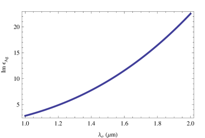
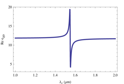
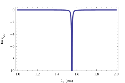
Figure 1: Real and imaginary parts of the relative permittivities $\epsilon_{Ag}$ and $\epsilon_{QD}$ plotted against free–space wavelength $\lambda_{o}$ ($\mu$m).

Herein, $\hbar\omega=0.8$ eV, $\hbar a=22.9$ meV, where $\hbar$ is the reduced Planck constant, the background relative permittivity $\epsilon_{b}=11.8$, and the broadening parameter $\gamma_{QD}=a/15.3$ [16]. The host dielectric material is taken to have the frequency–independent relative permittivity $\epsilon_{h}=3$. The real and imaginary parts of $\epsilon_{Ag}$ and $\epsilon_{QD}$ are plotted against free–space wavelength $\lambda_{o}\in\left[1,2\right]$ $\mu$m in Fig. 1. We see that $\mbox{Im}\,\epsilon_{QD}<0$ which indicates the quantum dots are active entities, particularly so at the resonance centred on $\lambda_{o}=1.55$ $\mu$m. From the point of view of the applicability of homogenization formalisms, there are two key points to notice: (i) the quantity

$$\delta=\frac{\mbox{Re}\,\epsilon_{Ag}}{\mbox{Re}\,\epsilon_{QD}}$$ (4)

is negative over the entire wavelength range considered; and (ii) we have $\left|\,\mbox{Re}\,\epsilon_{Ag}\,\right|\gg\left|\,\mbox{Im}\,\epsilon_{Ag}\,\right|$ for $\lambda_{o}\in\left[1,2\right]$ $\mu$m, and $\left|\,\mbox{Re}\,\epsilon_{QD}\,\right|\gg\left|\,\mbox{Im}\,\epsilon_{QD}\,\right|$ for $\lambda_{o}\in\left[1,1.55-\eta\right]\cup\left[1.55+\eta,2\right]$ $\mu$m where $\eta$ specifies a sharp resonance region centred on $\lambda_{o}=1.55$ $\mu$m. By analogy with dissipative HCMs [9, 10, 11], points (i) and (ii) suggest that the application of homogenization formalisms may be problematic.

2.2 Homogenization formalisms

The HCM is characterized by the relative permittivity dyadic

$$\underline{\underline{\epsilon}}^{HCM}=\epsilon^{HCM}_{t}\,\left(\,\underline{\underline{I}}-\hat{{\bf z}}\,\hat{{\bf z}}\right)+\epsilon^{HCM}_{z}\,\hat{{\bf z}}\,\hat{{\bf z}}.$$ (5)

We write ‘MG’ or ‘Br’ in lieu of ‘HCM’ according to whether the Maxwell Garnett or the Bruggeman estimate of $\underline{\underline{\epsilon}}^{HCM}$ is being considered. The anisotropy of the HCM arises due to the orientation of silver nanorods.

The Maxwell Garnett estimate of the relative permittivity dyadic is given explicitly by [17]

$$\underline{\underline{\epsilon}}^{MG}=\epsilon_{h}\underline{\underline{I}}+f_{Ag}\,\underline{\underline{a}}^{Ag/h}\mbox{ \tiny{${}^{\bullet}$} }\left(\underline{\underline{I}}-\frac{f_{Ag}}{3\epsilon_{h}}\,\underline{\underline{a}}^{Ag/h}\right)^{-1}+f_{QD}\,\underline{\underline{a}}^{QD/h}\mbox{ \tiny{${}^{\bullet}$} }\left(\underline{\underline{I}}-\frac{f_{QD}}{3\epsilon_{h}}\,\underline{\underline{a}}^{QD/h}\right)^{-1},$$ (6)

wherein the polarizability density dyadics

$$\underline{\underline{a}}^{\ell/h}=\left(\epsilon_{\ell}-\epsilon_{h}\right)\left[\,\underline{\underline{I}}+\left(\epsilon_{\ell}-\epsilon_{h}\right)\underline{\underline{D}}^{\ell/h}\right]^{-1},\qquad(\ell=Ag,QD),$$ (7)

and the depolarization dyadics [18]

$$\left.\begin{array}[]{l}\underline{\underline{D}}^{Ag/h}=\displaystyle{\frac{1}{2\epsilon_{h}}\,\left(\,\underline{\underline{I}}-\hat{{\bf z}}\,\hat{{\bf z}}\right)\vspace{4pt}}\\ \underline{\underline{D}}^{QD/h}=\displaystyle{\frac{1}{3\epsilon_{h}}\,\underline{\underline{I}}}\end{array}\right\}.$$ (8)

The Bruggeman estimate of the relative permittivity dyadic is given implicitly by [17]

$$f_{Ag}\,\underline{\underline{a}}^{Ag/Br}+f_{QD}\,\underline{\underline{a}}^{QD/Br}+f_{h}\,\underline{\underline{a}}^{h/Br}=\underline{\underline{0}}\,,$$ (9)

wherein the polarizability density dyadics

$$\underline{\underline{a}}^{\ell/Br}=\left(\epsilon_{\ell}\underline{\underline{I}}-\underline{\underline{\epsilon}}^{Br}\right)\mbox{ \tiny{${}^{\bullet}$} }\left[\,\underline{\underline{I}}+\underline{\underline{D}}^{\ell/Br}\mbox{ \tiny{${}^{\bullet}$} }\left(\epsilon_{\ell}\underline{\underline{I}}-\underline{\underline{\epsilon}}^{Br}\right)\right]^{-1},\qquad(\ell=Ag,QD,h),$$ (10)

and the depolarization dyadics [18, 19]

$$\left.\begin{array}[]{lcr}\underline{\underline{D}}^{Ag/Br}=\displaystyle{\frac{1}{2\epsilon_{t}^{Br}}\,\left(\,\underline{\underline{I}}-\hat{{\bf z}}\,\hat{{\bf z}}\right)}&&\vspace{4pt}\hfil\\ \underline{\underline{D}}^{\ell/Br}=\displaystyle{\frac{1}{\epsilon^{Br}_{t}}\,\left[\,\alpha L(\alpha)\left(\,\underline{\underline{I}}-\hat{{\bf z}}\,\hat{{\bf z}}\right)+L_{z}(\alpha)\,\hat{{\bf z}}\,\hat{{\bf z}}\right]}\,,&&(\ell=QD,h)\end{array}\right\}.$$ (11)

Herein, the scalar functions

$$\left.\begin{array}[]{l}L(\alpha)=\displaystyle{\frac{1}{2\alpha}\left\{F(\alpha)-\frac{1}{\alpha-1}\left[\,1-F(\alpha)\right]\right\}\vspace{4pt}}\\ L_{z}(\alpha)=\displaystyle{\frac{1}{\alpha-1}\left[\,1-F(\alpha)\right]}\end{array}\right\},$$ (12)

with

$$F(\alpha)=\frac{1}{\sqrt{\alpha-1}}\,\tan^{-1}\left(\sqrt{\alpha-1}\right)$$ (13)

and the scalar $\alpha=\epsilon^{Br}_{z}/\epsilon^{Br}_{t}$.

The relative permittivity dyadic $\underline{\underline{\epsilon}}^{Br}$ may be extracted from the nonlinear equation (9) by numerically. For example, the iterative scheme [7, 20]

$$\underline{\underline{\epsilon}}^{Br}_{\,(j)}=\mathcal{T}\left\{\underline{\underline{\epsilon}}^{Br}_{\,(j-1)}\right\},\qquad\qquad\left(\,j=1,2,3,\ldots\,\right),$$ (14)

wherein the operator $\mathcal{T}$ is defined as

$$\mathcal{T}\left\{\underline{\underline{\epsilon}}^{Br}\right\} = \Big{\{}f_{Ag}\,\epsilon_{Ag}\left[\,\underline{\underline{I}}+\underline{\underline{D}}^{Ag/Br}\mbox{ \tiny{${}^{\bullet}$} }\left(\epsilon_{Ag}\underline{\underline{I}}-\underline{\underline{\epsilon}}^{Br}\right)\right]^{-1}+f_{QD}\,\epsilon_{QD}\left[\,\underline{\underline{I}}+\underline{\underline{D}}^{QD/Br}\mbox{ \tiny{${}^{\bullet}$} }\left(\epsilon_{QD}\underline{\underline{I}}-\underline{\underline{\epsilon}}^{Br}\right)\right]^{-1}$$ (15)

$$+f_{h}\,\epsilon_{h}\left[\,\underline{\underline{I}}+\underline{\underline{D}}^{h/Br}\mbox{ \tiny{${}^{\bullet}$} }\left(\epsilon_{h}\underline{\underline{I}}-\underline{\underline{\epsilon}}^{Br}\right)\right]^{-1}\Big{\}}\mbox{ \tiny{${}^{\bullet}$} }\Big{\{}f_{Ag}\left[\,\underline{\underline{I}}+\underline{\underline{D}}^{Ag/Br}\mbox{ \tiny{${}^{\bullet}$} }\left(\epsilon_{Ag}\underline{\underline{I}}-\underline{\underline{\epsilon}}^{Br}\right)\right]^{-1}$$

$$f_{QD}\left[\,\underline{\underline{I}}+\underline{\underline{D}}^{QD/Br}\mbox{ \tiny{${}^{\bullet}$} }\left(\epsilon_{QD}\underline{\underline{I}}-\underline{\underline{\epsilon}}^{Br}\right)\right]^{-1}+f_{h}\left[\,\underline{\underline{I}}+\underline{\underline{D}}^{h/Br}\mbox{ \tiny{${}^{\bullet}$} }\left(\epsilon_{h}\underline{\underline{I}}-\underline{\underline{\epsilon}}^{Br}\right)\right]^{-1}\Big{\}}^{-1},$$

and the initial value

$$\underline{\underline{\epsilon}}^{Br}_{\,(0)}=\left(\,f_{Ag}\epsilon_{Ag}+f_{QD}\epsilon_{QD}+f_{h}\epsilon_{h}\,\right)\,\underline{\underline{I}}\,,$$ (16)

works sufficiently well for our purposes here.

2.3 Numerical estimates of the HCM permittivity

Let us begin by considering the Maxwell Garnett and Bruggeman estimates for an active HCM when the parameter $\delta$ is positive. This is achieved by setting $f_{Ag}=0$. Thus, the composite material comprises only quantum dots and the host dielectric material, and the resulting HCM is an isotropic dielectric material with relative permittivity dyadic $\epsilon^{HCM}\underline{\underline{I}}$. Estimates of the HCM relative permittivity computed using the Maxwell Garnett formalism and the Bruggeman formalism, namely $\epsilon^{MG}$ and $\epsilon^{Br}$ respectively, are plotted against $\lambda_{o}$ in Fig. 2, when $f_{QD}=0.3$. The Maxwell Garnett and Bruggeman estimates are similar, both qualitatively and quantitatively. For both formalisms, the HCM is active across the entire wavelength range considered, and its permittivity scalar exhibits a sharp resonance at $\lambda_{o}=1.55$ $\mu$m. Therefore, we infer that both the Maxwell Garnett and the Bruggeman formalisms are suitable for active HCMs with $\delta>0$.

Next we turn to the $\delta<0$ regime which is known to be problematic for dissipative HCMs [9, 10, 11]. In keeping with Bratkovsky et al. [14], we fix $f_{Ag}=0.063$ and $f_{QD}=0.3$; thus, $f_{h}$ is slightly reduced from its value for Fig. 2. In Fig. 3, the two entries in of the HCM’s relative permittivity dyadic, as computed using the Maxwell Garnett and Bruggeman formalisms, are plotted against $\lambda_{o}$. While the Maxwell Garnett and Bruggeman graphs in Fig. 3 are qualitatively similar, there are substantial quantitative differences. In particular, the imaginary part of $\epsilon^{Br}_{z}$ is more than 20 times larger than $\epsilon^{MG}_{z}$, apart from at the small resonance region centred on $\lambda_{o}=1.55$ $\mu$m. There are also substantial differences between Re $\epsilon^{Br}_{z}$ and Re $\epsilon^{MG}_{z}$. By comparison, the differences between $\epsilon^{Br}_{t}$ and $\epsilon^{MG}_{t}$ are relatively small.

For dissipative HCMs, the problematic nature of the $\delta<0$ regime is exacerbated as the imaginary parts of the constitutive parameters tend towards zero [9, 10, 11]. In order to investigate this issue for active HCMs, we repeated the computations of Fig. 3 with $\gamma_{Ag}$ and $\gamma_{QD}$ multiplied by $10^{-6}$. The corresponding plots of the real and imaginary parts of $\epsilon^{Br,MG}_{t,z}$ are presented in Fig. 4. The differences between the Maxwell Garnett estimates and the Bruggeman estimates are now enormous, especially between the imaginary parts of $\epsilon^{Br}_{z}$ and $\epsilon^{MG}_{z}$.

3 Concluding remarks

Our numerical studies reveal that the well–known homogenization formalisms named after Maxwell Garnett and Bruggeman appear to be fairly consistent, and provide physically plausible estimates, when applied to active isotropic dielectric HCMs, provided that the real parts of the relative permittivities of the component materials have the same sign. In contrast, if the real parts of the permittivities of the component materials have different signs then there are substantial differences between the estimates yielded by the two formalisms. These differences become enormous in the limiting case in which the imaginary parts of the relative permittivities of the component materials become vanishingly small.

For the particular homogenization scenario considered here, in the $\delta<0$ with $\gamma_{Ag,QD}\to 0$ regime, the HCM permittivity parameters estimated using the Bruggeman formalism have relatively large positive–valued imaginary parts away from the resonance region centred on $\lambda_{o}=1.55$ $\mu$m, and relatively large negative–valued imaginary parts at the resonance region centred on $\lambda_{o}=1.55$ $\mu$m. This is not physically plausible since it implies that the HCM is a strongly active material at the resonance region, and a strongly dissipative material away from the resonance region, in the limit wherein the component materials become inactive and nondissipative. Let us note that Bruggeman formalism arises as the lowest–order formulation of the strong–permittivity–fluctuation theory (SPFT) [22]. Accordingly, higher–order implementations of the SPFT are also subject to the limitations of the Bruggeman formalism. Furthermore, since the Maxwell Garnett and Bruggeman formalisms share a common provenance [23], doubt is also cast over the applicability of the Maxwell Garnett formalism for active HCMs with $\delta<0$ where the imaginary parts of the relative permittivities of the component materials are relatively small.

The present study extends and reinforces our previous studies which highlighted the limitations of conventional homogenization formalisms when applied to scenarios wherein the real parts of the constitutive parameters characterizing the component materials have different signs [9, 10, 11]. We see here that caution is needed for active HCMs as well as dissipative ones.

Acknowledgement: TGM thanks Dr Petter Holmström (KTH–Royal Institute of Technology, Sweden) for his helpful comments.

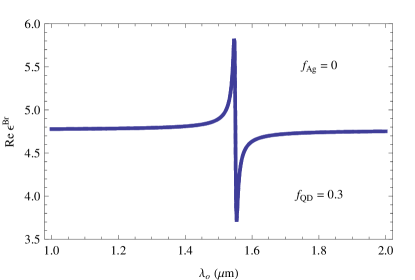
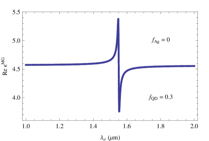
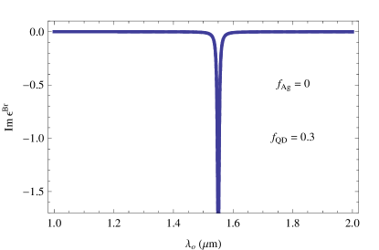
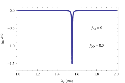
Figure 2: Bruggeman (left) and Maxwell Garnett (right) estimates of the HCM’s relative permittivity plotted against $\lambda_{o}$ ($\mu$m), with $f_{Ag}=0$ and $f_{QD}=0.3$.

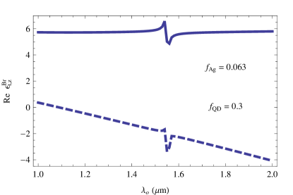
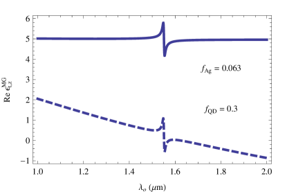
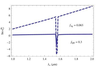
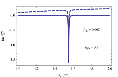
Figure 3: Bruggeman (left) and Maxwell Garnett (right) estimates of the two entries in the HCM’s relative permittivity dyadic plotted against $\lambda_{o}$ ($\mu$m), with $f_{Ag}=0.063$ and $f_{QD}=0.3$. The solid curves represent $\epsilon^{Br,MG}_{t}$ whereas the dashed curves represent $\epsilon^{Br,MG}_{z}$.

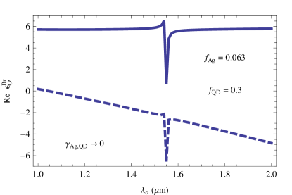
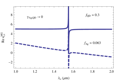
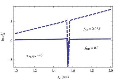
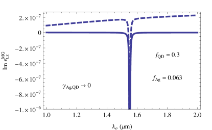
Figure 4: As Fig. 3 but with both $\gamma_{Ag}$ and $\gamma_{QD}$ multiplied by a factor of $10^{-6}$.

References

- [1] T. G. Mackay, J. Nanophoton. 2 (2008) 029503.
- [2] J. C. Maxwell Garnett, Phil. Trans. R. Soc. Lond. A 203 (1904) 385. (Reproduced in [8]).
- [3] G. B. Smith, J. Phys. D: Appl. Phys. 10 (1977) L39.
- [4] G. A. Niklasson, C. G. Granqvist, O. Hunderi, Appl. Opt. 20 (1981) 26.
- [5] D. A. G. Bruggeman, Ann. Phys. Lpz. 24 (1935) 636. (Reproduced in [8]).
- [6] A. V. Goncharenko, Phys. Rev. E 68 (2003) 041108. Corrections: 69 (2004) 029905.
- [7] T. G. Mackay, A. Lakhtakia, Opt. Commun. 259 (2006) 727.
- [8] A. Lakhtakia (Ed.), Selected Papers on Linear Optical Composite Materials, SPIE, Bellingham, WA, USA, 1996.
- [9] T. G. Mackay, A. Lakhtakia, Opt. Commun. 234 (2004) 35.
- [10] T. G. Mackay, J. Nanophoton. 1 (2007) 019501.
- [11] A. J. Duncan, T. G. Mackay, A. Lakhtakia, Opt. Commun. 271 (2007) 470.
- [12] T. G. Mackay, Electromagnetics 25 (2005) 461.
- [13] M. A. Noginov, J. Nanophoton. 2 (2008) 021855.
- [14] A. Bratkovsky, E. Ponizovskaya, S.–Y. Wang, P. Holmström, L. Thylén, Y. Fu, H. gren, Appl. Phys. Lett. 93 (2008) 193106.
- [15] C. F. Bohren, D. R. Huffman, Absorption and Scattering of Light by Small Particles, Wiley, New York, NY, USA, 1983.
- [16] P. Holmström. Personal communication (December 2008). Note that the parameter values of and we adopt here differ slightly from used for the computations described by Bratkovsky et al. [14] (who accidentally used a gain value which is too low).
- [17] T. G. Mackay, A. Lakhtakia, Prog. Optics 51 (2008) 121.
- [18] W. S. Weiglhofer, T. G. Mackay, IEEE Trans. Antennas Propagation. 50 (2002) 85.
- [19] B. Michel, Int. J. Appl. Electromagn. Mech. 8 (1997) 219.
- [20] B. Michel, in: O.N. Singh, A. Lakhtakia (Eds.), Electromagnetic Fields in Unconventional Materials and Structures, Wiley, New York, NY, USA, 2000, p. 39.
- [21] T. G. Mackay, A. Lakhtakia, W. S. Weiglhofer, Phys. Rev. E 62 (2000) 6052. Corrections: 63 (2001) 049901.
- [22] L. Tsang, J. A. Kong, Radio Sci. 16 (1981) 303. (Reproduced in [8]).
- [23] D. E. Aspnes, Am. J. Phys. 50 (1982) 704. (Reproduced in [8]).