Spin-1 Heisenberg antiferromagnetic chain with exchange and single-ion anisotropies

Abstract

Using density matrix renormalization group calculations, ground state properties of the spin-1 Heisenberg chain with exchange and single–ion anisotropies in an external field are studied. Our findings confirm and refine recent results by Sengupta and Batista, Physical Review Letters 99, 217205 (2007), on the same model applying Monte Carlo techniques. In particular, we present evidence for two types of biconical (or supersolid) and for two types of spin–flop (or superfluid) structures. Basic features of the quantum phase diagram may be interpreted qualitatively in the framework of classical spin models.

Recently, low-dimensional quantum anisotropic Heisenberg antiferromagnets have been shown to exhibit the analogue of the supersolid phase sen ; flora ; picon , usually denoted in magnetism as ’intermediate’, ’mixed’ or biconical koster phase, in which both order parameters of the bordering antiferromagnetic and spin–flop phases do not vanish. Indeed, already some decades ago, in 1956, Matsubara and Matsuda matsu pointed out the correspondence between quantum lattices and anisotropic Heisenberg models, when expressing Bose operators by spin operators. Using mean-field theory for calculating ground–state and thermal properties, supersolid or biconical structures have been observed in the uniaxially anisotropic XXZ Heisenberg antiferromagnets with additional single–site terms due to crystal–field anisotropies or with more–than–nearest neighbor interactions tsu ; liu (note that the mean-field approximation of the quantum models corresponds to that of classical models). Such phases may give rise to interesting multicritical behavior, especially, to tetracritical points aha ; folk .

In the last few years, biconical structures and phases in classical XXZ Heisenberg antiferromagnets with and without single–ion anisotropies in two as well as three dimensions have been studied using ground state considerations and Monte Carlo techniques hws ; hs ; bs .

Experimental evidence for biconical phases has been accumulated over the years bast ; smee ; zhou ; ng ; bog .

The current search for biconical phases in quantum magnets flora ; sen ; picon seems to be partly motivated by the fact that they are analogues to the supersolid phases wes ; schmidt ; nuss . Of course, it is also of much interest to study the impact of quantum fluctuations on the phases known to occur in classical anisotropic Heisenberg antiferromagnets in a magnetic field. In the following Note we shall address both aspects.

Specifically, we shall analyze ground state properties, $T=0$, of the spin–1 XXZ Heisenberg antiferromagnetic chain with a single–ion anisotropy in a field $B$. Using quantum Monte Carlo simulations, namely stochastic series expansions, for chains with periodic boundary conditions, Sengupta and Batista showed that its quantum phase diagram at zero temperature displays a field–induced supersolid phase sen . The model is described by the Hamiltonian

$${\cal H} = \sum\limits_{i}(J(S_{i}^{x}S_{i+1}^{x}+S_{i}^{y}S_{i+1}^{y}+\Delta S_{i}^{z}S_{i+1}^{z})$$ (1)

$${}+D(S_{i}^{z})^{2}-BS_{i}^{z})$$

where $i$ denotes the lattice sites. For $\Delta>1$ and $D>0$, the exchange and single–ion terms describe competing, uniaxial (along the direction of the field $B$, $B>0$, the $z$–direction) and planar anisotropies. Following the previous analysis sen , we shall deal with the case $D=\Delta/2$, restricting the analysis to the $(\Delta,B/J)$–plane.

To study the model, we here apply density matrix renormalization group (DMRG) techniques, yielding accurate results at zero temperature white ; scholl . In particular, we considered chains with open boundary conditions (allowing the study of fairly long chains). To monitor finite–size effects, the number of sites $L$ ranged from 15 up to 128. Usually, a random state was chosen as initial state. To get reliable data, typically up to 500 states during 120 sweeps were kept, with a total truncation error of $10^{-7}$ and a total energy variance of about $10^{-5}$.

At given chain length $L$, exchange anisotropy $\Delta$, and field $B/J$, the total magnetization $M=\sum\limits_{i}<S_{i}^{z}>$ follows from minimization of the energy $E(M,B)=E_{0}(M)-MB$, where $E_{0}(M)$ is the ground state energy at $B=0$ obtained from the DMRG calculations. Here and in the following, brackets, $<...>$, denote quantum mechanical expectation values. For fixed total magnetization various physical quantities of interest were determined, including the profile of the $z$–component of the magnetization, $m_{i}=<S_{i}^{z}>$, longitudinal and transverse correlators, $<S_{i}^{z}S_{i+r}^{z}>$ and, e.g., $<S_{i}^{x}S_{i+r}^{x}>$, as well as possible order parameters of the various structures and phases sen .

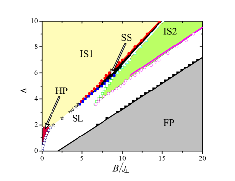
Figure 1: Ground state phase diagram of Hamiltonian (1) with $D=\Delta/2$, as has been obtained by Sengupta and Batistasen . $J_{\perp}$ in this figure is denoted by $J$ in the text.

According to the previous analysis sen , there are six distinct phases in the $(\Delta,B/J)$– plane at $T=0$, as depicted in Fig. 1. The Haldane phase (HP) hald occurs at small fields and anisotropies. Of course, the ferromagnetic (or normal fluid in quantum lattices) phase (FP) occurs for all anisotropies at sufficiently large fields. Furthermore, there are two solid tsu or Ising–like phases: The usual antiferromagnetic or Neel phase, the ’IS1’–phase in the notation of Sengupta and Batista, and, at rather large anisotropies, the ’IS2’–phase with $M\approx L/2$. Actually, the IS2–phase corresponds to the (10)–phase in the Ising–limit of Hamiltonian (1), the antiferromagnetic Blume–Capel model wang . The other two ground state phases are the superfluid tsu or spin–liquid sen (SL) phase, usually called in magnetism the spin–flop phase, and the supersolid tsu (SS) or biconical koster phase.

Indeed our analysis at selected values of $\Delta$, $3\leq\Delta\leq 7$, confirms the phase diagram sen , see Fig. 1. Moreover, we find evidence for two types of biconical as well as two types of spin–liquid structures. The evidence stems, especially, from the magnetization profiles, $m_{i}$. These profiles strongly depend on whether the number of sites, $L$, is odd or even, due to the open boundary conditions. In addition, finite–size effects may be important, when attempting to identify the ground state structures and transition points of the infinite chain.

Figure 2: Magnetization profiles $m_{i}$ for various total magnetizations $M$ in the SS phase in between the IS1 and IS2 phases at $\Delta$= 7 ($L=63$). The lower magnetizations belong to odd sites $i$, the upper ones to even sites. The profiles describe ground states in the range $10.1<B/J<10.7$

.

As illustrated in Figs. 2 and 3, for odd $L$, the biconical structures in between the IS1 and IS2 phases differ remarkably from those in between the IS1 and spin–flop phases. The first situation is exemplified in Fig. 2 for $\Delta=7$. We show magnetization profiles $m_{i}$ in the supersolid phase. Close to the center of the chain, i.e. in the ’bulk’, finite effects have been found to be weak. Increasing the total magnetization $M$ from 0 to about $L/2$ one encounters antiferromagnetic and supersolid ground states belonging to increasing fields $B/J$. In the bulk, $m_{i}$ is observed to stay close to one for odd sites $i$, while it changes to almost zero at the even sites on approach to the IS2 phase, $M\approx L/2$. One may describe that behavior in two ways: The spins on the odd sites always point in the field, or $z$, direction, while they turn, starting from –$z$ direction, in the IS1 phase more and more with larger values of $M$ towards the $xy$-plane on the even sites. Alternatively, one may interpret the behavior in the framework of the antiferromagnetic Blume–Capel chain. At $T=0$, there is a direct transition from the antiferromagnetic to the (10)–phase, fixing $D$ and enlargening the field. Along that transition line, there is a high degeneracy in configurations, where arbitrary fractions of spins in the state ’–1’ of the antiferromagnetic configuration are replaced by spins in the state ’0’. These degenerate structures seem to give rise to the biconical phase in the strongly anisotropic quantum Heisenberg model.

Figure 3: Magnetization profiles in the SS phase in between the IS1 and SL phases for various values of the total magnetization $M$, at $\Delta=5$ ($L=63$). The lower and upper values belong to odd and even sites, resp. The profiles describe ground states in the range $7.0<B/J<7.5$.

.

Attention may be drawn to the weak, but clearly visible modulations in the magnetization profiles in these supersolid structures, see Fig. 2.

Let us now consider the supersolid or biconical structures in between the IS1 and SL phases. Results for local magnetizations, $m_{i}$, are depicted in Fig. 3 for $\Delta=5$. Now, on approach to the SL phase, the magnetization, in the bulk, at the odd sites becomes much lower than one, and the difference between the local magnetizations $m_{i}$ in the center of the chain on odd and even sites is getting smaller and smaller. Such a behavior may be expected from classical anisotropic Heisenberg antiferromagnets tsu ; liu ; hs . Indeed, for the classical variant of Hamiltonian (1), the $z$–component of the local magnetization has been observed for biconical structures in between the antiferromagnetic and spin–flop phases to display a behavior similar to that found and seen here hs . The spins on both sublattices turn gradually and intercorrelated towards their common spin–flop orientation.

In contrast to the classical variant of the model, the transverse components of the spins show no long–range (antiferromagnetic) order in the quantum case. Instead, the transverse correlations seem to decay algebraically.

Of course, it would be interesting to clarify whether the two types of supersolid or biconical structures are separated by a sharp transition and to locate and charactarize that possible transition. Our preliminary results suggest that the SL phase seems to disappear at about $5<\Delta<5.5$, see also Fig 1. Note that in this region there are strong finite–size effects for the magnetization close to the center of the chain, and care is needed to discriminate SS and SL structures. For instance, at $\Delta=5.0$, we analyzed chains with up to 127 sites, identifying then the spin–flop phase. Actually, the possible transition between the two distinct supersolid structures may be argued to occur in that part of the phase diagram. Detailed investigations would require very long chains, and they are beyond the scope of this Note.

In the spin–liquid phase we observe different magnetization pattern for $M<L/2$ and for $M>L/2$, at all values of $\Delta$ we studied, i.e. independently of the SL phase being separated by the IS2 phase or not, see Fig. 1. In Figs. 4 and 5, magnetization profiles, $m_{i}$, illustrate both situations.

As exemplified in Fig.4, for $M<L/2$, the local magnetization displays an extended plateau in the center of the chain in the SL phase, similar to the behavior in the spin–flop phase for classical XXZ Heisenberg antiferromagnets without and with additional (competing) single–ion anisotropy hs . In Fig. 4 tiny modulations associated with odd and even sites are seen, which, however, are even reduced when considering longer chains, possibly, vanishing for infinite chains.

Figure 4: Magnetization profiles in the SL phase with $M<L/2$ ($L=63$) at $\Delta=3.5$. The fields of the corresponding ground states are in the range $5.0<B/J<5.8$.

Increasing $M$, $M>L/2$, but staying in the SL phase, the magnetization pattern changes significantly, as depicted in Fig. 5. One first observes a beat–like modulation about the mean magnetization, as being well known from superimposing two sine waves with slightly different wavelengths. The wavelength of the envelope of the beat is decreasing when enlargening $M$. Eventually, the modulation about the increasing mean value takes on a simple (nearly) sinusoidal form, with the wavelength getting larger and the amplitude getting smaller when increasing the total magnetization $M$. Of course, at $M=L$, the perfect ferromagnetic profile, with $M_{i}=1$ for all sites $i$, is reached. Going from the beat–like to the sinusoidal profiles, one increases systematically the average distance between successive extrema, reflecting, presumably, a quasi-continuous increase of the winding number of the modulation. Thence, it seems tempting to suggest the SL phase at $M>L/2$ to be of incommensurate type, while it seems to be of commensurate type for $M<L/2$. A similar distinction for the spin–flop phase may have been observed before in different parts of the phase diagram of Hamiltonian (1) sakai . It is worth mentioning that the amplitude of the modulations shrink somewhat for longer chains, and it would be interesting to analyze whether such, presumably, Friedel–like oscillations are still present in the infinite chain.

As in the case of the biconical phase, the transverse components of the magnetization show no long–range order in the SL phase of the quantum model sen ; mik ; schulz , in contrast to the situation in the classical variant of Hamiltonian (1).

Spin–flop phases with beat–like or sinusoidal modulations in $m_{i}$ do not occur in the classical variant of the Hamiltonian (1).

Again, a more detailed analysis, considering carefully finite–size effects, is desirable, but well beyond the scope of our present investigation.

Figure 5: Magnetization profiles $m_{i}$ in the SL phase with $M>L/2$ ($L=63$) at $\Delta=3.5$. The fields of the corresponding ground states are in the range $6.8<B/J<10.7$.

To summarize our findings, we have studied the S–1 antiferromagnetic XXZ Heisenberg antiferromagnetic chain with a competing, planar single–ion anisotropy. Using DMRG calculations, we confirmed and refined the ground state phase diagram obtained recently by Sengupta and Batista applying Monte Carlo techniques. In particular, we presented evidence for two distinct types of biconical or supersolid structures and for two distinct types of spin–flop or superfluid structures, in the finite chains we studied. We compared the findings with results on related classical magnets.

- (1) P. Sengupta and C. D. Batista, Phys. Rev. Lett. 99, 217205 (2007).
- (2) N. Laflorencie and F. Mila, Phys. Rev. Lett. 99, 027202 (2007).
- (3) J.- D. Picon, A. F. Albuquerque, K. P. Schmidt, N. Laflorencie, M. Troyer, and F. Mila, Phys. Rev. B 78, 184418 (2008).
- (4) J. M. Kosterlitz, D. R. Nelson, and M. E. Fisher, Phys. Rev. B 13, 412 (1976).
- (5) T. Matsubara and H. Matsuda, Prog. Theor. Phys. 16, 569 (1956)
- (6) H. Matsuda and T. Tsuneto, Prog. Theoret. Phys. Suppl. 46, 411 (1970).
- (7) K.-S. Liu and M. E. Fisher, J. Low. Temp. Phys. 10, 655 (1973).
- (8) A. Aharony, J. Stat. Phys. 110, 659 (2003).
- (9) R. Folk, Yu. Holovatch, and G. Moser, Phys. Rev. E 78, 041124 (2008).
- (10) M. Holtschneider, S. Wessel, and W. Selke, Phys. Rev. B 75, 224417 (2007).
- (11) M. Holtschneider and W. Selke, Phys. Rev. B 76, 220405(R) (2007); Eur. Phys. J. B 62, 147 (2008)
- (12) G. Bannasch and W. Selke, arXiv: 0807.1019
- (13) J. A. J. Basten, W. J. M. de Jonge, and E. Frikkee, Phys. Rev. B 21, 4090 (1980).
- (14) J. P. M. Smeets, E. Frikkee, and W. J. M. de Jonge, Phys. Rev. Lett. 49, 1515 (1982).
- (15) P. Zhou, G. F. Tuthill, and J. E. Drumheller, Phys. Rev. B 45, 2541 (1992).
- (16) K.- K. Ng and T. K. Lee, Phys. Rev. Lett. 97, 127204 (2006).
- (17) A. N. Bogdanov, A. V. Zhuravlev, and U. K. Roszler, Phys. Rev. B 75, 094425 (2007).
- (18) S. Wessel and M. Troyer, Phys. Rev. Lett. 95, 127205 (2005).
- (19) K. P. Schmidt, J. Dorier, A. M. Läuchli, and F. Mila, Phys. Rev. Lett. 100, 090401 (2008).
- (20) Z. Nussinov, Physics 1, 40 (2008).
- (21) S. R. White, Phys. Rev. B 48, 10345 (1993).
- (22) U. Schollwöck, Rev. Mod. Phys. 77, 259 (2005).
- (23) F. D. M. Haldane, Phys. Rev. Lett 50, 1153 (1983).
- (24) J. D. Kimel, P. A. Rikvold, and Y.-L. Wang, Phys. Rev. B 45, 7237 (1992).
- (25) T. Tonegawa, K. Okunishi, T. Sakai, and M. Kaburagi, Prog. Theor. Phys. Suppl. 159, 77 (2005).
- (26) H.-J. Mikeska and A. Kolezhuk, Lect. Notes Phys. 645, 1 (2004).
- (27) H. J. Schulz, Phys. Rev. B 34, 6372 (1986).