TUM-HEP-707/09 January 2009
TTP09-01
SFB/CPP-09-03
CERN-PH-TH/2008-204

The supersymmetric Higgs sector and $B\!-\!\,\overline{\!B}{}\,$ mixing for large $\tan\beta$

Martin Gorbahn¹,   Sebastian Jäger² ,  Ulrich Nierste³  and  Stéphanie Trine³

¹ Technische Universität München, Institute for Advanced Study,
Arcisstraße 21, D-80333 München, Germany

² Technische Universität München, Excellence Cluster “Universe”,
Boltzmannstraße 2, D-85748 Garching, Germany

³ Institut für Theoretische Teilchenphysik, Universität Karlsruhe, Karlsruhe Institute of Technology,
Engesserstraße 7, D-76128 Karlsruhe, Germany

Abstract

We match the Higgs sector of the most general flavour breaking and CP violating minimal supersymmetric standard model (MSSM) onto a generic two-Higgs-doublet model, paying special attention to the definition of $\tan\beta$ in the effective theory. In particular no $\tan\beta$-enhanced loop corrections appear in the relation to $\tan\beta$ defined in the $\overline{\textrm{DR}}$ scheme in the MSSM. The corrections to the Higgs-mediated flavour-changing amplitudes which result from this matching are especially relevant for the $B_{d}$ and $B_{s}$ mass differences $\Delta M_{d,s}$ for minimal flavour violation, where the superficially leading contribution vanishes. We give a symmetry argument to explain this cancellation and perform a systematic study of all Higgs-mediated effects, including Higgs loops. The corrections to $\Delta M_{s}$ are at most 7% for $\mu>0$ and $M_{A}<600\,\mbox{GeV}$ if constraints from other observables are taken into account. For $\mu<0$ they can be larger, but are always less than about 20%. Contrary to recent claims we do not find numerically large contributions here, nor do we find any $\tan\beta$-enhanced contributions from loop corrections to the Higgs potential in $B^{+}\to\tau^{+}\nu$ or $B\to X_{s}\gamma$. We further update supersymmetric loop corrections to the Yukawa couplings, where we include all possible CP-violating phases and correct errors in the literature. The possible presence of CP-violating phases generated by Higgs exchange diagrams is briefly discussed as well. Finally we provide improved values for the bag factors $P^{\rm VLL}_{1}$, $P^{\rm LR}_{2}$, and $P^{\rm SLL}_{1}$ at the electroweak scale.

PACS numbers: 11.30.Pb   12.60.Fr   12.15.Ff   14.40.Nd

1 Introduction

Supersymmetry constrains the structure of the Yukawa couplings of the minimal supersymmetric standard model (MSSM) to those of a special two-Higgs-doublet model (2HDM). In this 2HDM of type II one Higgs doublet, $H_{u}$, only couples to up-type fermions, while the other one, $H_{d}$, only couples to down-type fermions. As a consequence, there are no dangerous tree-level flavour-changing neutral current (FCNC) couplings of the neutral Higgs bosons. However, the presence of supersymmetry-breaking terms destroys this pattern at the one-loop level, permitting couplings of both Higgs doublets to all fermions. Thus the resulting Higgs sector is that of a general 2HDM, often called 2HDM of type III. As pointed out first by Hall, Rattazzi and Sarid, the loop-induced Yukawa couplings can compete with the tree-level ones in the limit of a large $\tan\beta=v_{u}/v_{d}$, which is the ratio of the vacuum expectation values (vevs) of $H_{u}$ and $H_{d}$ [1]: in the relationship between $H_{u,d}$-couplings and observed masses of the down-type fermions the loop suppression factor $\sim 0.02$ is offset by a factor of $\tan\beta$, so that ${\cal O}(1)$ corrections to the type-II 2HDM are possible for $\tan\beta\sim 50$. In such scenarios also ${\cal O}(1)$ loop-induced FCNC couplings of neutral Higgs bosons appear [2], which allow the branching fractions of (yet unobserved) leptonic $B$ decays to exceed their standard-model values by more than two orders of magnitude [3]. This observation has stimulated a large activity in flavour physics and powerful constraints on the MSSM Higgs sector in scenarios with large $\tan\beta$ have been derived from $B$ factory data [3, 4, 5, 6]. These Higgs-induced effects in flavour physics are very transparent in the limit

$$M_{\rm SUSY}\gg M_{A}\sim v\,,$$ (1)

where $M_{\rm SUSY}$ denotes the generic mass scale of the superpartners and the masses $M_{A}$, $M_{H}$, $M_{h}$ and $M_{H^{\pm}}$ of the five physical Higgs bosons are taken to be of the order of the electroweak scale $v\equiv\sqrt{v_{u}^{2}+v_{d}^{2}}=246\,\,\mbox{GeV}$. All low-energy observables can be computed in the type-III 2HDM, which emerges as the effective theory in the limit of Eq. (1). The new couplings can be calculated from finite one-loop diagrams with supersymmetric particles and thus become functions of the MSSM parameters, so that the desired constraints on the supersymmetric parameter space can be derived. The effective 2HDM Lagrangian efficiently incorporates all large-$\tan\beta$ effects, equivalent to a perturbative all-order resummation of those radiative corrections which are enhanced by a factor of $\tan\beta$ [7].

$B_{q}\!-\!\,\overline{\!B}{}_{q}\,$ mixing (with $q=d$ or $s$) plays a special role among the FCNC transitions of $B$ mesons. Here the leading new effect stems from effective tree-level diagrams with neutral Higgs bosons (see Fig. 1).

 

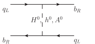
Figure 1: Leading contributions to $B_{q}\!-\!\,\overline{\!B}{}_{q}\,$ mixing from supersymmetric Higgs bosons. The FCNC couplings are induced by supersymmetric loops. The coefficient of $Q_{1}^{\rm SLL}=(\overline{b}_{R}q_{L})(\overline{b}_{R}q_{L})$ vanishes, if the tree-level relations between Higgs masses and mixing angles are used.

 

A priori the dominant contribution is expected from Yukawa couplings to right-handed $b$ quarks, generating the effective $\Delta B=2$ operator

$$Q_{1}^{\rm SLL} \equiv \left(\overline{b}_{R}q_{L}\right)\left(\overline{b}_{R}q_{L}\right)\,.$$ (2)

However, the corresponding coefficient $C_{1}^{\rm SLL}$ vanishes exactly, if one employs the tree-level relations between the Higgs masses and mixing angles [2]. Nevertheless, sizeable effects in $B_{s}\!-\!\,\overline{\!B}{}_{s}\,$ mixing are possible even in scenarios with minimal flavour violation (MFV) [8, 9, 10, 11, 12, 13, 14, 15, 16], in which the Cabibbo-Kobayashi-Maskawa (CKM) matrix [17] is the only source of flavour violation: keeping the strange Yukawa coupling non-zero one finds a non-vanishing contribution to the coefficient of

$$Q_{2}^{\rm LR}\equiv\left(\overline{b}_{R}q_{L}\right)\left(\overline{b}_{L}q_{R}\right)\,,$$ (3)

which depletes the $B_{s}\!-\!\,\overline{\!B}{}_{s}\,$ mass difference $\Delta M_{s}$ [5]. The tree-level vanishing of $C_{1}^{\rm SLL}$ calls for a systematic analysis of all subleading effects. In particular, the contribution that stems from $Q^{\rm SLL}_{1}$ can a priori compete with the contribution of the operator $Q^{\rm LR}_{2}$ above if the one-loop corrections to the MSSM Higgs potential [18, 19, 20, 21, 23, 22, 24] are taken into account. While a lot of work has been devoted to the analysis of the Yukawa sector [2, 3, 7, 5, 6], little attention has been given to effects from the Higgs potential. An exception is Ref. [25], which finds large contributions. We revisit these effects in the present paper and perform a systematic matching of the MSSM Higgs sector onto the type-III 2HDM. The result is not only relevant for the calculation of $C_{1}^{\rm SLL}$, it also clarifies the relationship between the definitions of $\tan\beta$ in the MSSM and the effective 2HDM. This is important to link the constraints from flavour physics to other fields of MSSM phenomenology, in particular Higgs physics. Our paper is organized as follows. We derive the corrected $B\!-\!\,\overline{\!B}{}\,$ mixing amplitude in Sect. 2, including all relevant subleading contributions. The renormalization of $\tan\beta$ and som further technial issues are the subject of Sect. 3. In Sect. 4 we apply our new formulae to the phenomenology of $B\!-\!\,\overline{\!B}{}\,$ mixing, analysing the mass differences $\Delta M_{d}$ and $\Delta M_{s}$ as well as CP-violation. Our results are summarized in Sect. 5. We list our notation and our technical results in four appendices. Parts of our results were previously presented by one of us at a conference [38].

2 Higgs-mediated effects in $B\!-\!\,\overline{\!B}{}\,$ mixing

The quantity governing the $B_{q}\!-\!\,\overline{\!B}{}_{q}\,$ mass difference is the off-diagonal element of the $B_{q}\!-\!\,\overline{\!B}{}_{q}\,$ meson mass matrix: $\Delta M_{q}=2\left|M_{21}^{q}\right|$, with

$$M_{21}^{q}=\frac{\left\langle\overline{B}_{q}\left|\mathcal{H}_{\rm eff}^{\Delta B=2}\right|B_{q}\right\rangle}{2M_{B_{q}}}\,.$$ (4)

The $\Delta B=2$ effective weak Hamiltonian $\mathcal{H}_{\rm eff}^{\Delta B=2}$ consists in general of eight dimension-six operators:

$$\mathcal{H}_{\rm eff}^{\Delta B=2}=\frac{G_{F}^{2}M_{W}^{2}\lambda_{qb}^{2}}{16\pi^{2}}\sum_{i=1}^{8}C_{i}(\mu_{h})Q_{i}(\mu_{h})\,,$$ (5)

with $\lambda_{qb}\equiv V_{tq}V_{tb}^{\ast}$. The set of operators in Eq. (5) comprises the standard-model operator,

$$Q_{1}^{\rm VLL}=\left(\overline{b}_{L}\gamma_{\mu}q_{L}\right)\left(\overline{b}_{L}\gamma^{\mu}q_{L}\right)\,,$$ (6)

the two scalar operators defined in Eqs. (2) and (3), the operator

$$Q_{1}^{\rm SRR} \equiv \left(\overline{b}_{L}q_{R}\right)\left(\overline{b}_{L}q_{R}\right)\,,$$ (7)

and four other operators. The complete list of operators plus the relevant evanescent operators is given in Eq. (140) and Eq. (141) of Appendix C. We express our results in terms of matrix elements at the high scale $\mu_{h}$ which we choose equal to the top mass $\overline{m}_{t}(\overline{m}_{t})=164\,\mbox{GeV}$. In this way the other four operators do not appear in our formulae. However, some of them are needed to connect $Q_{i}(\mu_{h})$ with $Q_{i}(\mu_{b})$ at the low scale $\mu_{b}\sim m_{b}$ at which their matrix elements are computed, because they mix with $Q_{1}^{\rm SLL}$, $Q_{1}^{\rm SRR}$ or $Q_{2}^{\rm LR}$ under renormalization. We follow the conventions of Refs. [26] and [27] for operators and matrix elements. In particular we parametrize the hadronic matrix elements as

$$\left\langle\overline{B}_{q}\left|Q_{i}(\mu_{h})\right|B_{q}\right\rangle=\frac{2}{3}M_{B_{q}}^{2}f_{B_{q}}^{2}P_{i}\,.$$ (8)

The $P_{i}$’s are obtained [27] by renormalization-group evolution from the conventional bag factors $B_{i}$ computed at the low scale $\mu_{b}$. We calculate the $P_{i}$’s from up-to-date lattice QCD results in Appendix C, where we fully exploit constraints from heavy-quark relations. This is a new feature of our analysis compared to previous studies of new-physics effects in $B\!-\!\,\overline{\!B}{}\,$ mixing.

2.1 Effective tree-level Higgs exchange

The Higgs sector of the MSSM contains two $SU(2)$ doublets $H_{u}$ and $H_{d}$,

$$H_{u}=\binom{h_{u}^{+}}{h_{u}^{0}}\,,\qquad H_{d}=\epsilon\binom{h_{d}^{+}}{h_{d}^{0}}^{\ast}\,,\qquad\epsilon=\left(\begin{array}[c]{cc}0&1\\ -1&0\end{array}\right)\,,$$ (9)

of hypercharge $+1/2$ and $-1/2$, respectively, with vacuum expectation values (vevs) $\langle h_{u,d}^{0}\rangle=v_{u,d}/\sqrt{2}$ of relative size $\tan\beta=v_{u}/v_{d}$. Integrating out supersymmetric particles, the Lagrangian of the resulting effective 2HDM is no longer restricted to be of type II, and is constrained only by the electroweak symmetry. Neither will it be renormalizable, with operators of dimension greater than four encoding effects that decouple at least as $v/M_{\rm SUSY}$ for heavy superpartners. We begin with a short review of some pertinent aspects of the general 2HDM.

Defining

$$\left(\begin{array}[]{c}\Phi\\ \Phi^{\prime}\end{array}\right)=\left(\begin{array}[]{cc}\cos\beta&\sin\beta\\ -\sin\beta&\cos\beta\end{array}\right)\,\left(\begin{array}[]{c}-\epsilon H_{d}^{*}\\ H_{u}\end{array}\right)\,,$$ (10)

the most general fermion-Higgs interactions up to dimension four read

$$\begin{split}{\cal L}_{Y}=&-\frac{\sqrt{2}}{v}\bar{d}_{Ri}\,M_{d_{ij}}\,\Phi^{\dagger}Q_{Lj}-\bar{d}_{Ri}\,\kappa_{ij}\,\Phi^{\prime\dagger}Q_{Lj}\\ &-\frac{\sqrt{2}}{v}\bar{u}_{Ri}\,M_{u_{ij}}\,Q_{Lj}\cdot\!\Phi-\bar{u}_{Ri}\,\tilde{\kappa}_{ij}Q_{Lj}\cdot\!\Phi^{\prime}+\textrm{h.c.}\,,\end{split}$$ (11)

where we have employed the notation $a\cdot b\equiv a^{T}\epsilon\,b$. By construction, the vev of $\Phi^{\prime}$ vanishes, whereas $\Phi$ has $\langle\Phi\rangle=(0,v/\sqrt{2})^{T}$ and contains all three Goldstone bosons. Hence only $\Phi$ can contribute to the fermion masses and only $\Phi^{\prime}$ can have flavour-violating neutral couplings. The flavour basis is defined such that the down-quark mass matrix $M_{d}$ is diagonal. In this basis the FCNC Higgs couplings to $b$-quarks are governed by $\kappa_{bq}$ or $\kappa_{qb}$ ($q=d$ or $s$).

The renormalizable Higgs self-interactions are comprised in the most general gauge-invariant dimension-four two-Higgs-doublet potential [28],

$$V\underset{}{=}m_{11}^{2}H_{d}^{\dagger}H_{d}+m_{22}^{2}H_{u}^{\dagger}H_{u}+\left\{m_{12}^{2}H_{u}\cdot H_{d}+h.c.\right\}$$

$$+\frac{\lambda_{1}}{2}(H_{d}^{\dagger}H_{d})^{2}+\frac{\lambda_{2}}{2}(H_{u}^{\dagger}H_{u})^{2}+\lambda_{3}(H_{u}^{\dagger}H_{u})(H_{d}^{\dagger}H_{d})+\lambda_{4}(H_{u}^{\dagger}H_{d})(H_{d}^{\dagger}H_{u})$$

$$+\left\{\frac{\lambda_{5}}{2}\left(H_{u}\cdot H_{d}\right)^{2}-\lambda_{6}(H_{d}^{\dagger}H_{d})\left(H_{u}\cdot H_{d}\right)-\lambda_{7}(H_{u}^{\dagger}H_{u})\left(H_{u}\cdot H_{d}\right)+\mbox{h.c.}\right\}.$$ (12)

The couplings $m_{12}^{2}$, $\lambda_{5}$, $\lambda_{6}$, and $\lambda_{7}$ are in general complex, yet the vevs $v_{u,d}$ can be made real by a $U(1)$ transformation on the Higgs fields. The definitions of $m^{2}_{ij}$ and $\lambda_{i}$ in Eq. (12) coincide with Ref. [28] except for $\lambda_{3}$ and $\lambda_{4}$: we associate a different operator with $\lambda_{4}$ to eliminate it from tree-level neutral-Higgs phenomenology and have instead $\lambda_{3}=\lambda_{3}^{\text{{\cite[cite]{[\@@bibref{}{Haber:1997dt}{}{}]}}}}+\lambda_{4}^{\text{{\cite[cite]{[\@@bibref{}{Haber:1997dt}{}{}]}}}}$ and $\lambda_{4}=-\lambda_{4}^{\text{{\cite[cite]{[\@@bibref{}{Haber:1997dt}{}{}]}}}}$.

Shifting the fields in Eq. (12) by their vevs, which minimize $V$ at tree level,

$$h_{u,d}^{0}=\frac{1}{\sqrt{2}}(v_{u,d}+\phi_{u,d}+i\chi_{u,d})\,,$$ (13)

determines the physical Higgs-boson mass matrices and interactions. We write the neutral-Higgs mass matrix in the basis $(\phi_{d},\phi_{u},\chi_{d},\chi_{u})$ in terms of $2\times 2$ blocks,

$$M^{2}_{0}=\left(\begin{array}[]{cc}M^{2}_{R}&M^{2}_{RI}\\[5.69054pt] M^{2\,T}_{RI}&M^{2}_{I}\end{array}\right)\,,$$ (14)

with $M^{2}_{R}$, $M^{2}_{RI}$, and $M^{2}_{I}$ given in Eqs. (23-26) below. In the CP-conserving case, $M^{2}_{RI}=0$, and $M^{2}_{R}$ and $M^{2}_{I}$ are diagonalized by rotating the CP-even and CP-odd Higgs fields through angles $\alpha$ and $\beta$, respectively:

$$\left(\begin{array}[c]{c}\phi_{d}\\ \phi_{u}\end{array}\right)=\left(\begin{array}[c]{cc}\cos\alpha&-\sin\alpha\\ \sin\alpha&\cos\alpha\end{array}\right)\left(\begin{array}[c]{c}H^{0}\\ h^{0}\end{array}\right),\quad\left(\begin{array}[c]{c}\chi_{d}\\ \chi_{u}\end{array}\right)=\left(\begin{array}[c]{cc}\cos\beta&-\sin\beta\\ \sin\beta&\cos\beta\end{array}\right)\left(\begin{array}[c]{c}G^{0}\\ A^{0}\end{array}\right).$$ (15)

The same angle $\beta=\arctan v_{u}/v_{d}$ as defined above appears because (and only when) $v_{u}$, $v_{d}$ minimize $V$. If CP violation is present, four physical mixing angles $\alpha_{1,2,3}$ and $\beta$ are required to diagonalize $M_{0}^{2}$. The charged-Higgs mass matrix $M_{+}^{2}$ is always diagonalized by $\beta$,

$$\left(\begin{array}[c]{c}h_{d}^{+}\\ h_{u}^{+}\end{array}\right)=\left(\begin{array}[c]{cc}\cos\beta&-\sin\beta\\ \sin\beta&\cos\beta\end{array}\right)\left(\begin{array}[c]{c}G^{+}\\ H^{+}\end{array}\right).$$ (16)

The non-standard effective operators $Q_{2}^{\rm LR}$, $Q_{1}^{\rm SLL}$, and $Q_{1}^{\rm SRR}$ are generated at tree level via the exchange of neutral Higgs bosons (see Fig. 1) with the Wilson coefficients

$$C_{2}^{\rm LR}=-\frac{8\pi^{2}}{G_{F}^{2}M_{W}^{2}\lambda_{qb}^{2}}\left(\kappa_{qb}^{\ast}\,\kappa_{bq}\right)\mathcal{F}^{+},\qquad C_{1}^{\rm SLL}=-\frac{4\pi^{2}}{G_{F}^{2}M_{W}^{2}\lambda_{qb}^{2}}\left(\kappa_{bq}\right)^{2}\mathcal{F}^{-},$$ (17)

and $C^{\rm SRR}_{1}$ obtained from $C^{\rm SLL}_{1}$ through the replacement $\left(\kappa_{bq}\right)^{2}\mathcal{F}^{-}\to\left(\kappa_{qb}^{\ast}\right)^{2}\mathcal{F}^{-\ast}$. We find that, in the general case, the Higgs propagation factors can be expressed as follows:

$$\mathcal{F}^{+} =\frac{\det\left(M_{R}^{2}+M_{I}^{2}+iM_{RI}^{2}-iM_{RI}^{2\,T}\right)}{m_{1}^{2}m_{2}^{2}m_{3}^{2}}\equiv\frac{\det B}{m_{1}^{2}m_{2}^{2}m_{3}^{2}},$$ (18)

$$\mathcal{F}^{-} =-\frac{\det\left(M_{R}^{2}-M_{I}^{2}-iM_{RI}^{2}-iM_{RI}^{2\,T}\right)}{m_{1}^{2}m_{2}^{2}m_{3}^{2}}\equiv-\frac{\det A}{m_{1}^{2}m_{2}^{2}m_{3}^{2}},$$ (19)

where the denominators contain the product of the three nonzero eigenvalues of $M^{2}_{0}$. In the CP-conserving case, Eqs. (18) and (19) reduce to the well-known expressions

$$\mathcal{F}^{\pm}=\frac{\sin^{2}(\alpha-\beta)}{M_{H}^{2}}+\frac{\cos^{2}(\alpha-\beta)}{M_{h}^{2}}\pm\frac{1}{M_{A}^{2}}\,,$$ (20)

where $M_{A}$ denotes the CP-odd Higgs-boson mass.

The discussion so far has been completely general. Particularizing to the MSSM, a perturbative matching calculation relates the two theories. At tree level this trivially results in

$$M^{(0)}_{d} =\frac{v}{\sqrt{2}}\cos\beta\,Y_{d}, M^{(0)}_{u} =\frac{v}{\sqrt{2}}\sin\beta\,Y_{u},$$ (21)

$$\kappa^{(0)} =-\sin\beta\,Y_{d}, \tilde{\kappa}^{(0)} =\cos\beta\,Y_{u}$$

$$m_{11}^{2^{(0)}} =\left|\mu\right|^{2}+m_{H_{d}}^{2}\equiv m_{1}^{2}, \lambda_{1}^{(0)} =\lambda_{2}^{(0)}=-\lambda_{3}^{(0)}=(g^{2}+g^{\prime 2})/4\equiv\tilde{g}^{2}/4,$$

$$m_{22}^{2^{(0)}} =\left|\mu\right|^{2}+m_{H_{u}}^{2}\equiv m_{2}^{2}, \lambda_{4}^{(0)} =g^{2}/2,$$

$$m_{12}^{2^{(0)}} =B\mu, \lambda_{5}^{(0)} =\lambda_{6}^{(0)}=\lambda_{7}^{(0)}=0.$$

At this order $\kappa^{(0)}$ and $\tilde{\kappa}^{(0)}$ are aligned with $M_{d}^{(0)}$ and $M_{u}^{(0)}$, respectively, so that no FCNC are induced, as it must be in a model II. At one loop, all couplings in Eq. (12) are generated. Moreover, the corrections to the Yukawa couplings have the more general form

$$M^{(1)}_{d}=\frac{v}{\sqrt{2}}\cos\beta\big{[}\Delta Y_{d}+\tan\beta\,\Delta K\big{]},\qquad\kappa^{(1)}=-\sin\beta\,\big{[}\Delta Y_{d}-\cot\beta\Delta K\big{]},$$ (22)

where $\Delta Y_{d_{ij}}$ and $\Delta K_{ij}$ parametrize the one-loop vertices $\bar{d}_{Ri}H_{d}\cdot Q_{Lj}$ and $\bar{d}_{Ri}H_{u}^{\dagger}Q_{Lj}$, respectively. Diagonalizing $M_{d}$ rotates $\kappa^{(0)}$, giving rise to a flavour-violating coupling $\propto Y_{d}\tan\beta/(16\,\pi^{2})$, which can be of ${\cal O}(1)$ for $\tan\beta\sim 50$.

The origin of this explicit $\tan\beta$ enhancement (in addition to the mere presence of large down-type Yukawa couplings), which can compensate the loop factor $1/(16\,\pi^{2})$, is the replacement of $v_{d}$ by $v_{u}\gg v_{d}$ in the contribution of $\Delta K$ to $M_{d}$ [1]. This removal of a $v_{d}$ suppression can happen only in dimensionful quantities. In the fermion mass terms, only one power of $\tan\beta$ can appear because there was only one power of $v_{d}$ to begin with. This is in agreement with the findings in [7]. Our approach using un-shifted Higgs fields (“unbroken-theory”) makes particularly evident that this result holds to all orders, as the Yukawa Lagrangian only involves dimensionless couplings and there are no hidden factors of $\tan\beta$. Although we have integrated out only the sparticles – as we assume a hierarchy $v,M_{A}\ll M_{\rm SUSY}$ – the argument continues to hold if we also integrate over the Higgs fields, keeping only constant background values of $\Phi,\Phi^{\prime}$ (spurions). The reason is that for determining the mass matrices, the relevant external four-momenta are of ${\cal O}(m_{q})$, providing an expansion parameter $m_{q}/v$ or $m_{q}/M_{A}$. Hence the Higgs contributions to the effective potential (which on general grounds respects the electroweak symmetry) can be organized into a (local) effective Lagrangian, with $m_{q}$-suppressed corrections to the form Eq. (11) encoded in higher-dimensional operators with additional derivatives acting on $d_{Ri}$ or $Q_{Lj}$. The contribution from both Higgs and sparticle loops to $M_{d}$ is then simply obtained upon substituting for $\Phi,\Phi^{\prime}$ their vacuum expectation values. This mass matrix is to be identified with a short-distance (such as $\overline{\rm MS}$) mass in the effective QCD $\times$ QED at low energies, where the dependence on the chosen scheme cancels against the explicit form of the matching (of the 2HDM onto QCD $\times$ QED).

There is only one other place where a similar $\tan\beta$ enhancement can occur, namely in the dimensionful self-couplings of the (shifted) Higgs fields, that is, their masses and trilinear couplings. Indeed, at dimension two it is exhibited in the neutral Higgs mass matrix Eq. (14). Explicitly, one has (with $s_{\beta}\equiv\sin\beta$, $c_{\beta}\equiv\cos\beta$, and $\lambda_{k}^{r}\equiv{\rm Re}\,\lambda_{k}$)

$$M_{R}^{2}=v^{2}\left(\begin{array}[c]{cc}\lambda_{5}^{r}s_{\beta}^{2}+2\lambda_{6}^{r}s_{\beta}c_{\beta}+\lambda_{1}c_{\beta}^{2}&\lambda_{7}^{r}s_{\beta}^{2}+\lambda_{3}s_{\beta}c_{\beta}+\lambda_{6}^{r}c_{\beta}^{2}\\ \lambda_{7}^{r}s_{\beta}^{2}+\lambda_{3}s_{\beta}c_{\beta}+\lambda_{6}^{r}c_{\beta}^{2}&\lambda_{2}s_{\beta}^{2}+2\lambda_{7}^{r}s_{\beta}c_{\beta}+\lambda_{5}^{r}c_{\beta}^{2}\\ \end{array}\right)+M^{2}_{I}\,,$$ (23)

$$M_{I}^{2}=M_{A}^{2}\left(\begin{array}[c]{cc}s_{\beta}^{2}&-s_{\beta}c_{\beta}\\ -s_{\beta}c_{\beta}&c_{\beta}^{2}\end{array}\right)\,,$$ (24)

where $(m_{12}^{2})^{r}$ has been traded for $M_{A}^{2}$, with

$$s_{\beta}\,c_{\beta}\,M_{A}^{2}=(m_{12}^{2})^{r}-\frac{v^{2}}{2}(\lambda_{7}^{r}\,s_{\beta}^{2}+2\lambda_{5}^{r}\,s_{\beta}c_{\beta}+\lambda_{6}^{r}\,c_{\beta}^{2}).$$ (25)

If CP is conserved, in the limit of infinite $\tan\beta$ ($c_{\beta}\to 0$) the leading mass splitting $M_{H}^{2}-M_{A}^{2}=\lambda_{5}v^{2}$, and the leading correction to the tree-level result $\alpha=0$ is determined by $\lambda_{7}$. In the former case, an enhancement by two powers of $\tan\beta$ occurs ($M_{H}^{2}-M_{A}^{2}={\cal O}(\cos^{2}\beta)$ at tree level), while the loop correction to $\alpha$ is enhanced by a single power of $\tan\beta$ with respect to its tree-level value. Either effect is sufficient to remove the cancellation in ${\cal F}^{-}$ in Eq. (20). Moreover, a $1/\tan\beta$-unsuppressed CP-violating contribution proportional to $\lambda_{5}^{i}$ and $\lambda_{7}^{i}$ appears to occur:

$$M_{RI}^{2}=\frac{v^{2}}{2}\left(\begin{array}[c]{cc}\lambda_{5}^{i}\,s_{\beta}^{2}\,+\,2\lambda_{6}^{i}\,s_{\beta}c_{\beta}&-\lambda_{5}^{i}\,s_{\beta}c_{\beta}\,-\,2\lambda_{6}^{i}\,c_{\beta}^{2}\\ 2\lambda_{7}^{i}\,s_{\beta}^{2}\,+\,\lambda_{5}^{i}\,s_{\beta}c_{\beta}&-2\lambda_{7}^{i}\,s_{\beta}c_{\beta}\,-\,\lambda_{5}^{i}\,c_{\beta}^{2}\end{array}\right),$$ (26)

where $\lambda_{k}^{i}\equiv{\rm Im}\,\lambda_{k}$. However, as we show in Sect. 2.3 below, the individual phases of $\lambda_{5}$ and $\lambda_{7}$ become unphysical in the limit $\tan\beta\to\infty$, and mixing between the CP-even and CP-odd sectors is described by a single angle $\alpha^{\prime}$, determined by the relative phase of $\lambda_{5}$ and $\lambda_{7}^{2}$. Finally, the charged Higgs mass matrix is given by

$$M_{+}^{2}=\left(1+\frac{v^{2}\left(\lambda_{4}+\lambda_{5}^{r}\right)}{2M_{A}^{2}}\right)\text{ }M_{I}^{2}.$$ (27)

Here no $\tan\beta$ enhancement due to loop-induced couplings occurs.

Unlike the case of the fermion mass matrix, the typical momentum flowing through the effective Lagrangian Eq. (12) for an on-shell Higgs is itself of ${\cal O}(v)$ or ${\cal O}(M_{A})$. Hence Higgs-loop contributions to the Higgs masses cannot be included in Eq. (12), but rather the full effective action would be needed. Higgs-loop effects in $\kappa_{bq}$ and $\kappa_{qb}$ multiplying ${\cal F}^{\pm}$ could, however, be included via Eq. (11), since again the momenta flowing through the vertices are much smaller than $v$, $M_{A}$. This is not possible in Higgs boxes, where large momenta flow through the FCNC vertices. We will present a systematic method to include all Higgs-loop contributions in Sect. 2.3.

It is instructive to consider the explicit form of the numerator in Eq. (19), which is

$$\det A\;= \;v^{4}\Big{[}(\lambda_{2}\lambda_{5}^{*}-\lambda_{7}^{*2})\,s^{4}_{\beta}+2\,(\lambda_{2}\lambda_{6}^{*}-\lambda_{3}\lambda_{7}^{*}+\lambda_{5}^{*}\lambda_{7})\,s^{3}_{\beta}c_{\beta}$$

$$+(\lambda_{1}\lambda_{2}-\lambda_{3}^{2}+|\lambda_{5}|^{2}-2\lambda_{6}\lambda_{7}^{*}+4\lambda_{6}^{*}\lambda_{7})\,s^{2}_{\beta}c^{2}_{\beta}$$

$$+2(\lambda_{5}\lambda_{6}^{*}-\lambda_{3}\lambda_{6}+\lambda_{1}\lambda_{7})s_{\beta}c^{3}_{\beta}+(\lambda_{1}\lambda_{5}-\lambda_{6}^{2})c^{4}_{\beta}\Big{]}.$$ (28)

With Eq. (21), $\det A=v^{4}\,(\lambda_{1}\lambda_{2}-\lambda_{3}^{2})\,s^{2}_{\beta}c^{2}_{\beta}=0$, reproducing the known vanishing of ${\cal F}^{-}$ employing the tree-level MSSM Higgs sector. The cancellation is removed already at the leading-logarithmic level. For instance, $\lambda_{2}$ alone receives a large additive correction $\propto y_{t}^{4}$ due to top-quark loops, which is also responsible for the most important correction to the tree-level mass of $h$. The corresponding corrections could be computed by RG-evolving the tree-level couplings in the effective 2HDM. However, as we are considering large $\tan\beta$, we expect (and find below) the most important effect to be due to $\lambda_{5}$ and $\lambda_{7}$, which remove the ${\cal O}(c^{2}_{\beta})$ suppression of the leading-log result, as anticipated above.

2.2 The case of minimal flavour violation

From the discussion so far it follows that $|{\cal F}^{+}|={\cal O}(1/M_{A}^{2})\gg|{\cal F}^{-}|={\cal O}(1/(16\pi^{2}M_{A}^{2}))$, implying $|C_{2}^{\rm LR}|\gg|C_{1}^{\rm SLL}|$ for generic $\kappa_{ij}$, such that the motivation to consider ${\cal F}^{-}$ at all is not very strong. The situation is fundamentally different for MFV because then the contribution proportional to ${\cal F}^{+}$ turns out to be suppressed by a light quark mass, introducing a further small parameter $m_{q}/m_{b}$ comparable to $1/(16\pi^{2})$ or $1/\tan\beta$ for $q=s$ (and negligible for $q=d$). For simplicity, in this paper we consider the simplest version of MFV, assuming flavour-universal soft breaking terms $\tilde{m}^{2}_{Q}$, $\tilde{m}^{2}_{u}$ and $\tilde{m}^{2}_{d}$ and trilinear SUSY-breaking terms $T_{u_{ij}}$, $T_{d_{ij}}$ which are proportional to the Yukawa matrices and therefore diagonal in the super-CKM basis (denoted with a hat): $\hat{T}_{u_{ij}}=a_{t}y_{u_{i}}\delta_{ij}$ and $\hat{T}_{d_{ij}}=a_{b}y_{d_{i}}\delta_{ij}$, see Appendix A for details of our notation. The structure of our results, however, does not depend on these additional assumptions. The $\tan\beta$-enhanced loop-induced FCNC couplings of the neutral Higgs bosons in Eq. (11) can be expressed as:

$$\kappa_{bq} = \epsilon_{Y}\text{ }y_{t}^{2}\lambda_{qb}\frac{\sqrt{2}\,m_{b}}{v\cos^{2}\beta}\frac{1}{1+\widetilde{\epsilon}_{3}\tan\beta}\frac{1}{1+\epsilon_{0}\tan\beta}\,,$$ (29)

$$\kappa_{qb} = \epsilon_{Y}\text{ }y_{t}^{2}\lambda_{qb}^{*}\frac{\sqrt{2}\,m_{q}}{v\cos^{2}\beta}\frac{1}{1+\widetilde{\epsilon}_{3}\tan\beta}\frac{1}{1+\epsilon_{0}\tan\beta}\,,$$ (30)

with $y_{t}=\sqrt{2}m_{t}/(v\sin\beta)$ and $\lambda_{qb}=V_{tq}V_{tb}^{*}$. The effective couplings $\epsilon_{Y}$, $\epsilon_{0}$ and $\widetilde{\epsilon}_{3}$, which depend on the MSSM parameters, have been analysed in the decoupling limit $M_{\rm SUSY}\gg v$ in the limit $g=g^{\prime}=0$ in Refs. [2, 3, 4] for the case that $\epsilon_{Y}$, $\epsilon_{0}$ and $\widetilde{\epsilon}_{3}$ are real. We consider the general case allowing $\mu$, the universal trilinear term $a_{t}$ and the gaugino mass parameters to be complex. Effects from non-zero $g,g^{\prime}$ have been taken into account in Ref. [5], where also effects beyond the decoupling limit were considered. The corresponding expressions for $M_{\rm SUSY}\gg v$, suited for our analysis, were derived in Ref. [25]. We have recalculated the FCNC couplings of neutral Higgs bosons including all CP-violating phases and found agreement with the results for the FCNC self-energies given in Ref. [5], but encountered a significant discrepancy with Ref. [25]. In our results, the phase conventions of the first five parameters can be inferred from Eqs. (98) and (105) of Sect. A. The phase convention for $M_{3}$ complies with that of $M_{1,2}$ and the gluino mass equals $M_{\widetilde{g}}=|M_{3}|$. Of course one can choose one of these parameters (e.g. $M_{3}$) real. Now the effective couplings of Eqs. (29) and (30) read:

$$\epsilon_{0} =\frac{-2\alpha_{s}}{3\pi}\frac{\mu^{*}}{M_{3}}H_{2}\left(\frac{M_{\widetilde{b}L}^{2}}{|M_{3}|^{2}},\frac{M_{\widetilde{b}R}^{2}}{|M_{3}|^{2}}\right)$$

$$+\frac{g^{\prime 2}}{96\pi^{2}}\frac{\mu^{*}}{M_{1}}\left[H_{2}\left(\frac{M_{\widetilde{b}L}^{2}}{|M_{1}|^{2}},\frac{|\mu|^{2}}{|M_{1}|^{2}}\right)+2H_{2}\left(\frac{M_{\widetilde{b}R}^{2}}{|M_{1}|^{2}},\frac{|\mu|^{2}}{|M_{1}|^{2}}\right)\right]$$

$$+\frac{g^{\prime 2}}{144\pi^{2}}\frac{\mu^{*}}{M_{1}}H_{2}\left(\frac{M_{\widetilde{b}L}^{2}}{|M_{1}|^{2}},\frac{M_{\widetilde{b}R}^{2}}{|M_{1}|^{2}}\right)+\frac{3\,g^{2}}{32\pi^{2}}\frac{\mu^{*}}{M_{2}}H_{2}\left(\frac{M_{\widetilde{b}L}^{2}}{|M_{2}|^{2}},\frac{|\mu|^{2}}{|M_{2}|^{2}}\right),$$ (31)

$$\epsilon_{Y} =\frac{-1}{16\pi^{2}}\frac{a_{t}^{*}}{\mu}H_{2}\left(\frac{M_{\widetilde{t}L}^{2}}{|\mu|^{2}},\frac{M_{\widetilde{t}R}^{2}}{|\mu|^{2}}\right)\;+\;\epsilon_{Y,v/M}\,,$$ (32)

$$\widetilde{\epsilon}_{3} =\epsilon_{0}+y_{t}^{2}\epsilon_{Y}\,.$$ (33)

Here

$$H_{2}(x,y)=\frac{x\log x}{(1-x)(x-y)}+\frac{y\log y}{(1-y)(y-x)}.$$ (34)

Numerically, the electroweak contributions in $\epsilon_{0}$ can be of ${\cal O}(10\%)$. They improve the comparison with the results computed with full chargino and squark mass matrices (see Eq. (5.1) in the second paper in [5]).

Ref. [5] also discusses threshold corrections to the fermion kinetic operators (wave function renormalizations). While these terms are not $\tan\beta$-enhanced, the flavour-diagonal quark wave function renormalization constants receive sizable contributions from squark-gluino loops. One can parametrize these loops in terms of a new quantity $\epsilon_{0}|_{\rm kin}$ which will add to $\epsilon_{0}$ in the relation between the MSSM Yukawa coupling $y_{d_{i}}$ and the physical quark mass $m_{d_{i}}$ (see Eq. (108) for the case of the bottom Yukawa coupling). $\epsilon_{0}|_{\rm kin}$ will likewise appear in the relation between $\kappa_{ij}$ and $y_{d_{i}}$, but it drops out once $\kappa_{ij}$ is expressed in terms of $m_{d_{i}}$, so that it does not appear in Eqs. (29) and (30). This cancellation of the flavour-diagonal quark wave function renormalization can be verified by inserting Eq. (2.29) into Eq. (2.26) of the second paper in [5]. This feature can be traced back to the fact that the wave function renormalization affects both the tree-level and the loop-induced Yukawa couplings with the same multiplicative factor.

Comparing our result with Ref. [25], we find different results for $\epsilon_{0}$ and $\epsilon_{Y}$: In Ref. [25] the chargino-stop contribution proportional to $g^{2}$ is erroneously assigned to $\epsilon_{Y}$ rather than $\epsilon_{0}$. Since this piece does not contain any Yukawa couplings (the chargino is a pure wino here), all three generations contribute in the same way and the resulting overall CKM structure combines to $V_{ub}^{*}V_{uq}+V_{cb}^{*}V_{cq}+V_{tb}^{*}V_{tq}$, which is zero for $q\neq b$ and equal to one for $q=b$. This GIM cancellation eliminates the wino-stop loop from $\epsilon_{Y}$, while this loop contributes to $\epsilon_{0}$ twice as much as the corresponding loop with a neutral wino-like neutralino and a sbottom. The two terms are combined into the last term in Eq. (31). Omitting the chargino loop here would violate SU(2) gauge symmetry, which also enforces $\widetilde{t}_{L}=\widetilde{b}_{L}$ in the decoupling limit. Since $\epsilon_{Y}$ normalises all Higgs-induced FCNC couplings, one should verify the accuracy of the $M_{\rm SUSY}\gg v$ limit: It is easy to include the $\tan\beta$-enhanced contributions to $\epsilon_{Y}$ to all orders in $v/M_{\rm SUSY}$. To this end one merely has to calculate the FCNC $\overline{b}_{R}q_{L}$ self-energy using the exact chargino and up-squark mass eigenstates. This self-energy renormalises the off-diagonal pieces of the quark mass matrix and cause the mismatch between the flavour structures of the latter with the Yukawa couplings leading to $\epsilon_{Y}\neq 0$. In higher loop-orders $\tan\beta$-enhanced contributions are suppressed by products of small CKM elements (and are negligible) or are flavour-conserving and therefore contribute to $\epsilon_{0}$ rather than to $\epsilon_{Y}$. Using the $\overline{b}_{R}q_{L}$ self-energy $\left(\Sigma^{d}_{mL}\right)^{3i}$ (with $q=d_{i}$) from Ref. [5] one finds

$$\begin{split}\epsilon_{Y,v/M}=&\frac{1}{16\pi^{2}}\frac{a_{t}^{*}}{\mu}H_{2}\left(\frac{M_{\widetilde{t}L}^{2}}{|\mu|^{2}},\frac{M_{\widetilde{t}R}^{2}}{|\mu|^{2}}\right)\;+\;\frac{\sqrt{2}}{vy_{t}^{2}\lambda_{bd_{i}}}\frac{\left(\Sigma^{d}_{mL}\right)^{3i}}{y_{b}}\end{split}$$ (35)

(Note that $\left(\Sigma^{d}_{mL}\right)^{3i}\propto y_{b}$ and be aware of the different sign conventions for $y_{b}$ in Eq. (108) and Ref. [5].) We stress that Eq. (35) must be evaluated for $i\neq 3$, so that the GIM cancellation of the above-mentioned wino-stop loop takes place. Numerically one finds a marginal impact of $\epsilon_{Y,v/M}$: Setting all supersymmetric massive parameters equal to a common value $M_{\rm SUSY}$, one finds that $\epsilon_{Y,v/M}$ amounts to a mere 1.4% correction to $\epsilon_{Y}$ for $M_{\rm SUSY}=400\,\mbox{GeV}$. Even for $M_{\rm SUSY}=150\,\mbox{GeV}$, for which the expansion in $v/M_{\rm SUSY}$ formally breaks down, $\epsilon_{Y,v/M}$ depletes $\epsilon_{Y}$ by as little as 8%. $\epsilon_{Y,v/M}$ also enters $\epsilon_{0}$ through Eq. (32). It can be inferred from Ref. [7] that this procedure indeed leads to the correct all-order resummation of the $\tan\beta$-enhanced corrections involving $y_{t}$. Corrections to $\epsilon_{0}$ beyond the $M_{\rm SUSY}\gg v$ limit from $g,g^{\prime}$ and $y_{b}$ are considered in Refs. [7] and [5]. We remark that no terms proportional to $y_{b}^{2}$ occur in Eqs. (31–33), because the corresponding loops violate hypercharge and involve a suppression factor of $v^{2}/M_{\rm SUSY}^{2}$.

We verify from Eqs. (29) and (30) that $\kappa_{qb}^{*}\kappa_{bq}$ multiplying ${\cal F}^{+}$ in Eq. (17) is suppressed by a factor $m_{q}/m_{b}$ relative to $\kappa_{bq}^{2}$, which multiplies ${\cal F}^{-}$. Hence $C_{1}^{\rm SLL}$ is naively leading (over $C_{2}^{\rm LR}$) from the point of view of MFV alone, and a meaningful analysis of $B_{q}-\overline{B}_{q}$ mixing requires a systematic investigation of all leading corrections to its vanishing “tree” value. (The coefficient $C_{1}^{\rm SRR}$ both undergoes a strong $m_{q}^{2}/m_{b}^{2}$ suppression and involves ${\cal F}^{-*}$, and can thus be disregarded.) It is then useful to think of the $\Delta F=2$ amplitude as being a function of the four small parameters identified so far:

$$l\equiv\frac{1}{(4\pi)^{2}},\quad\omega\equiv\frac{m_{q}}{m_{b}},\quad\frac{1}{\tan\beta},\quad\nu=\frac{v}{M_{\rm SUSY}}.$$ (36)

The vanishing 2HDM tree diagram for ${\cal F}^{-}$ is (superficially) ${\cal O}((\cot\beta)^{-2}\,l^{2}\,\nu^{0}\,\omega^{0})$, i.e. ${\cal O}(1)$ when treating all expansion parameters on the same footing. Conversely, ${\cal F}^{+}$ is nonzero at the tree level but is suppressed by one power of $\omega$, which is non-negligible only for $q=s$. We have already seen that ${\cal F}^{-}$ vanishes exactly for tree-level matching (or up to ${\cal O}(1/\tan^{2}\beta)$ when including leading logs), so there are no ${\cal O}(1/\tan\beta)$ corrections at first subleading order. This leaves loop corrections (via sparticle corrections to the $\lambda_{i}$ as well as loops in the effective 2HDM) and possible corrections due to higher-dimensional operators, not written in Eqs. (11) and (12). We now discuss these contributions in turn.

Sparticle loops

One-loop contributions from higgsinos, gauginos, and sfermions correct the values of $\lambda_{1,2,3.4}$ in Eq. (12) and induce non-zero couplings $\lambda_{5,6,7}$. As a technical result of our paper, we have computed the $\lambda_{i}$ for general sparticle masses and flavour structure. These results are reported in Appendix B. At tree-level in the effective theory and in the leading order of $1/\tan\beta$ the quantitiy ${\cal F^{-}}$ receives only contributions from $\lambda_{2}$, $\lambda_{5}$, and $\lambda_{7}$, cf. Eq. (2.1). The general results of Eqs. (3.1),(121),(125),(126),(128), (130-131), and (133) for the MFV case read

$$\begin{split}\lambda_{7}=\bar{\lambda}_{7}=&\frac{1}{16\pi^{2}}\Bigg{\{}\frac{1}{4}\mu a_{\tau}|y_{\tau}|^{2}\left(2g^{\prime^{2}}C_{0}\left(\tilde{m}_{l},\tilde{m}_{e},\tilde{m}_{e}\right)+\left(g^{2}-g^{\prime^{2}}\right)C_{0}\left(\tilde{m}_{e},\tilde{m}_{l},\tilde{m}_{l}\right)\right)\\ &+\mu a_{\tau}|\mu|^{2}|y_{\tau}|^{4}D_{0}\left(\tilde{m}_{e},\tilde{m}_{e},\tilde{m}_{l},\tilde{m}_{l}\right)\\ &-\frac{1}{4}\tilde{g}^{2}\mu\bigg{(}3a_{b}|y_{b}|^{2}B^{\prime}_{0}\left(\tilde{m}_{d},\tilde{m}_{Q}\right)+3a_{t}|y_{t}|^{2}B^{\prime}_{0}\left(\tilde{m}_{u},\tilde{m}_{Q}\right)+a_{\tau}|y_{\tau}|^{2}B^{\prime}_{0}\left(\tilde{m}_{e},\tilde{m}_{l}\right)\bigg{)}\\ &+g^{4}\left(3\mu M_{2}\tilde{D}_{2}\left(|M_{2}|,|M_{2}|,|\mu|,|\mu|\right)-\frac{3}{4}\mu|M_{2}|B^{\prime}_{0}\left(|M_{2}|,|\mu|\right)\right)\\ &-\frac{1}{4}g^{2}g^{\prime^{2}}\mu\bigg{(}|M_{1}|B^{\prime}_{0}\left(|M_{1}|,|\mu|\right)+3|M_{2}|B^{\prime}_{0}\left(|M_{2}|,|\mu|\right)\\ &\qquad\qquad-4\left(M_{1}+M_{2}\right)\tilde{D}_{2}\left(|M_{1}|,|M_{2}|,|\mu|,|\mu|\right)\bigg{)}\\ &+g^{\prime^{4}}\left(\mu M_{1}\tilde{D}_{2}\left(|M_{1}|,|M_{1}|,|\mu|,|\mu|\right)-\frac{1}{4}\mu|M_{1}|B^{\prime}_{0}\left(|M_{1}|,|\mu|\right)\right)\Bigg{\}}\,,\end{split}$$ (37)

$$\begin{split}\lambda_{5}=\bar{\lambda}_{5}=&-\frac{1}{16\pi^{2}}\mu^{2}\bigg{\{}3a_{b}^{2}\left|y_{b}\right|{}^{4}D_{0}\left(\tilde{m}_{d},\tilde{m}_{d},\tilde{m}_{Q},\tilde{m}_{Q}\right)+3a_{t}^{2}\left|y_{t}\right|{}^{4}D_{0}\left(\tilde{m}_{Q},\tilde{m}_{Q},\tilde{m}_{u},\tilde{m}_{u}\right)\\ &+a_{\tau}^{2}\left|y_{\tau}\right|{}^{4}D_{0}\left(\tilde{m}_{e},\tilde{m}_{e},\tilde{m}_{l},\tilde{m}_{l}\right)-3g^{4}M_{2}^{2}D_{0}\left(\left|M_{2}\right|,\left|M_{2}\right|,|\mu|,|\mu|\right)\\ &-2g^{2}g^{\prime^{2}}M_{1}M_{2}D_{0}\left(\left|M_{1}\right|,\left|M_{2}\right|,|\mu|,|\mu|\right)-g^{\prime^{4}}M_{1}^{2}D_{0}\left(\left|M_{1}\right|,\left|M_{1}\right|,|\mu|,|\mu|\right)\bigg{\}}\,,\end{split}$$ (38)

and

$$\begin{split}\lambda_{2}=\bar{\lambda}_{2}=&\frac{\tilde{g}^{2}}{4}+\frac{1}{16\pi^{2}}\Bigg{\{}-\frac{3}{4}g^{\prime^{4}}B_{0}\left(\tilde{m}_{e},\tilde{m}_{e}\right)-\frac{3}{8}\left(g^{4}+g^{\prime^{4}}\right)B_{0}\left(\tilde{m}_{l},\tilde{m}_{l}\right)\\ &+\frac{1}{2}\left(g^{\prime^{2}}-g^{2}\right)|\mu y_{\tau}|^{2}C_{0}\left(\tilde{m}_{e},\tilde{m}_{l},\tilde{m}_{l}\right)-g^{\prime^{2}}|\mu y_{\tau}|^{2}C_{0}\left(\tilde{m}_{l},\tilde{m}_{e},\tilde{m}_{e}\right)\\ &-|\mu y_{\tau}|^{4}D_{0}\left(\tilde{m}_{e},\tilde{m}_{e},\tilde{m}_{l},\tilde{m}_{l}\right)\\ &-\frac{1}{4}g^{\prime^{4}}B_{0}\left(\tilde{m}_{d},\tilde{m}_{d}\right)+\left(-3|y_{t}|^{4}+2g^{\prime^{2}}|y_{t}|^{2}-g^{\prime^{4}}\right)B_{0}\left(\tilde{m}_{u},\tilde{m}_{u}\right)\\ &+\frac{1}{8}\left(-9g^{4}-24|y_{t}|^{4}-g^{\prime^{4}}-4|y_{t}|^{2}\left(g^{\prime^{2}}-3g^{2}\right)\right)B_{0}\left(\tilde{m}_{Q},\tilde{m}_{Q}\right)\\ &+\frac{1}{2}\left(3g^{2}-12|y_{t}|^{2}-g^{\prime^{2}}\right)|a_{t}y_{t}|^{2}C_{0}\left(\tilde{m}_{Q},\tilde{m}_{Q},\tilde{m}_{u}\right)\\ &+2\left(g^{\prime^{2}}-3|y_{t}|^{2}\right)|a_{t}y_{t}|^{2}C_{0}\left(\tilde{m}_{Q},\tilde{m}_{u},\tilde{m}_{u}\right)-g^{\prime^{2}}|\mu y_{b}|^{2}C_{0}\left(\tilde{m}_{Q},\tilde{m}_{d},\tilde{m}_{d}\right)\\ &-\frac{1}{2}\left(3g^{2}+g^{\prime^{2}}\right)|\mu y_{b}|^{2}C_{0}\left(\tilde{m}_{d},\tilde{m}_{Q},\tilde{m}_{Q}\right)\\ &-3|a_{t}y_{t}|^{4}D_{0}\left(\tilde{m}_{Q},\tilde{m}_{Q},\tilde{m}_{u},\tilde{m}_{u}\right)-3|\mu y_{b}|^{4}D_{0}\left(\tilde{m}_{d},\tilde{m}_{d},\tilde{m}_{Q},\tilde{m}_{Q}\right)\\ &+\frac{1}{2}\tilde{g}^{2}\left(3|\mu y_{b}|^{2}B^{\prime}_{0}\left(\tilde{m}_{d},\tilde{m}_{Q}\right)+|\mu y_{\tau}|^{2}B^{\prime}_{0}\left(\tilde{m}_{e},\tilde{m}_{l}\right)+3|a_{t}y_{t}|^{2}B^{\prime}_{0}\left(\tilde{m}_{u},\tilde{m}_{Q}\right)\right)\\ &+\frac{1}{24}\left[-2\log\frac{\tilde{m}_{d}^{2}}{\mu_{0}^{2}}g^{\prime^{4}}-6\log\frac{\tilde{m}_{e}^{2}}{\mu_{0}^{2}}g^{\prime^{4}}-8\log\frac{\tilde{m}_{u}^{2}}{\mu_{0}^{2}}g^{\prime^{4}}\right.\\ &\qquad\qquad\left.-3\log\frac{\tilde{m}_{l}^{2}}{\mu_{0}^{2}}\left(g^{4}+g^{\prime^{4}}\right)-\log\frac{\tilde{m}_{Q}^{2}}{\mu_{0}^{2}}\left(9g^{4}+g^{\prime^{4}}\right)\right]\\ &-\frac{1}{24}g^{4}\left[-12\tilde{D}_{2}\left(|M_{2}|,|M_{2}|,|\mu|,|\mu|\right)|M_{2}|^{2}-60\tilde{D}_{4}\left(|M_{2}|,|M_{2}|,|\mu|,|\mu|\right)\right.\\ &\qquad\qquad\left.+9W\left(|M_{2}|,|\mu|\right)+4\log\frac{|\mu|^{2}}{\mu_{0}^{2}}+8\log\frac{M_{2}^{2}}{\mu_{0}^{2}}+14\right]\\ &-\frac{1}{8}g^{2}g^{\prime^{2}}\left[-8{\rm Re}\left(M_{1}M_{2}^{*}\right)\tilde{D}_{2}\left(|M_{1}|,|M_{2}|,|\mu|,|\mu|\right)-8\tilde{D}_{4}\left(|M_{1}|,|M_{2}|,|\mu|,|\mu|\right)\right.\\ &\qquad\qquad\left.+W\left(|M_{1}|,|\mu|\right)+3W\left(|M_{2}|,|\mu|\right)+4\right]\\ &-\frac{1}{24}g^{\prime^{4}}\left[-12\tilde{D}_{2}\left(|M_{1}|,|M_{1}|,|\mu|,|\mu|\right)|M_{1}|^{2}-12\tilde{D}_{4}\left(|\mu|,|\mu|,|M_{1}|,|M_{1}|\right)\right.\\ &\qquad\qquad\left.+3W\left(|M_{1}|,|\mu|\right)+4\log\left(\frac{|\mu|^{2}}{\mu_{0}^{2}}\right)+6\right]\Bigg{\}}\,,\end{split}$$ (39)

where the loop functions $B_{0}$, $C_{0}$, $D_{0}$, $B^{\prime}_{0}$, $\tilde{D}_{2}$, $\tilde{D}_{2}$, and $W$ are defined in Appendix B.4, and the notation $\bar{\lambda}_{i}$ refers to the matching scheme as explained in Sect. 3. Inspecting Eq. (2.1), $\lambda_{7}$ enters quadratically, which formally is of higher loop order. Nevertheless, it can be seen that $\lambda_{7}^{2}\propto y_{t}^{8}$ as opposed to $\lambda_{2}\lambda_{5}^{*}\propto\tilde{g}^{2}y_{t}^{4}$, which can partly offset the additional loop suppression. Indeed we find that, numerically, neglecting $\lambda_{7}$ is not always a good approximation (Sect. 4).

The form of the matching result depends on the renormalization schemes of both the full theory, i.e., the MSSM, and the effective theory, i.e., the 2HDM. The latter cancels in physical quantities, while explicit MSSM scheme dependence cancels against the one implicit in the MSSM parameters, to ensure that the couplings in the effective theory are independent of the renormalization of the MSSM at any given order of perturbation theory. The residual scheme dependence in both cases may, however, be important as we are considering a leading effect. We will discuss scheme issues in Sect. 3.1, paying special attention to the definitions of $\tan\beta$.

Higgs loops

There is a considerable number of one-loop diagrams in the effective 2HDM that can contribute to $B\!-\!\,\overline{\!B}{}\,$ mixing amplitudes (Fig. 2, upper row).

 

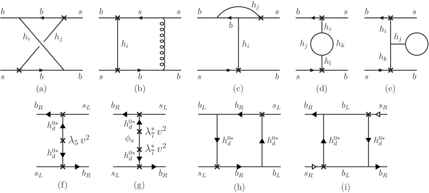
Figure 2: Upper row: A subset of one-loop diagrams for $B_{q}-\bar{B}_{q}$ mixing in the effective two-Higgs-doublet model. Lower row: Tree and one-loop diagrams contributing at large $\tan\beta$ when employing the Lagrangian ${\cal L}_{\rm ltb}$ and tree-level couplings. The crosses denote the flavor-changing neutral Higgs couplings and (in diagrams (f) and (g)) loop-suppressed Higgs mass terms. On the lower row, arrows designate the flow of the conserved $U(1)$ charge discussed in Sect. 2.3

 

These give the following contributions to the Wilson coefficients multiplying $Q^{\rm VLL}_{1}$ and $Q^{\rm VRR}_{1}$:

$$C^{\rm VLL}_{1}|_{\rm{Higgs\,loops}} = -\frac{1}{4}\frac{m_{b}^{2}}{v^{2}\cos^{2}\beta(1+\widetilde{\epsilon}_{3}^{*}\tan\beta)^{2}}\frac{\kappa_{bq}^{2}}{G_{F}^{2}M_{W}^{2}\lambda_{qb}^{2}}C_{0}(M_{A}^{2},M_{A}^{2},0)\,,$$ (40)

$$C^{\rm VRR}_{1}|_{\rm Higgs\,loops} = -\frac{1}{4}\frac{m_{b}^{2}}{v^{2}\cos^{2}\beta(1+\widetilde{\epsilon}_{3}\tan\beta)^{2}}\frac{\kappa_{qb}^{*2}}{G_{F}^{2}M_{W}^{2}\lambda_{qb}^{2}}C_{0}(M_{A}^{2},M_{A}^{2},0)\,.$$ (41)

In these expressions, we have neglected the small Yukawa coupling $y_{q}$ and employed tree-level MSSM mass relations, in agreement with our approximation of working to leading order in small parameters (in the present case, the loop factor $1/(16\pi^{2})$). $C^{\rm VRR}_{1}$ is suppressed by two powers of $m_{q}/m_{b}$ inside $\kappa_{qb}^{*2}$ in the MFV case, hence beyond our accuracy. The results Eqs. (40) and (41) involve a great deal of cancellations, which can be understood in terms of symmetry arguments, as explained in Sect. 2.3 below. We note the absence of charged-Higgs contributions in the approximation considered here.

$v/M$-suppressed effects

All of the couplings given in Eq. (11) correspond to the zeroth order in the $v/M_{\rm SUSY}$ expansion, or equivalently to the level of dimension-four operators. Gauge invariance forbids dimension-five operators built from quark and Higgs fields, so the leading higher-dimensional operators have dimension six. This can lead to more general Higgs-fermion couplings than those deriving from Eq. (11) and, in consequence, the cancellation leading to $C^{\rm SLL}_{1}=0$ might be broken. To see that this is indeed the case, consider the operator

$$Q^{(6)}=\frac{1}{M_{\rm SUSY}^{2}}(H_{u}^{\dagger}H_{u})(\bar{b}_{R}H_{u}^{\dagger}Q_{L}),$$ (42)

which gives rise, inter alia, to effective dimension-three and -four couplings

$$\frac{2\sqrt{2}\,v_{u}^{3}}{M_{\rm SUSY}^{2}}\,\bar{b}_{R}s_{L}+\frac{2\,v_{u}^{2}}{M_{\rm SUSY}^{2}}(\bar{b}_{R}s_{L}h_{u}^{0}+2\,\bar{b}_{R}s_{L}h_{u}^{0*}).$$ (43)

The first term is removed by a rediagonalization of the quark mass matrices, but the two remaining terms, in general, are not. The appearance of $h_{u}^{0}$ in addition to $h_{u}^{0*}$ leads to a contribution to $C_{1}^{\rm SLL}$ proportional to $\kappa_{bq}\,C^{(6)}$. However, because of $R$-parity, SUSY particles do not contribute to tree graphs with external standard particles only, such that $Q^{(6)}$ (or any other higher-dimension operator) is only induced at the loop level, and this loop-suppression factor is not compensated by factors of $\tan\beta$. (Recall that the ${\cal O}(1)$ FCNC couplings at dimension four are nothing but rotated tree-level Yukawa couplings.) Hence any $v/M_{\rm SUSY}$ corrections that break the cancellation in ${\cal F}^{-}$ involve an additional loop suppression, and can be neglected for the present analysis. On the other hand, as Eq. (43) shows, the higher-dimensional operators do have an impact on the rediagonalization of the quark mass matrices and, consequently, on the size of the FCNC couplings $\kappa_{bq}$. These effects preserve the cancellations in ${\cal F}^{-}$ discussed above but have a mild impact on the FCNC couplings multiplying ${\cal F}^{+}$ in $C_{2}^{\textrm{LR}}$ (cf Eq. (35) and the discussion around it).

2.3 $U(1)_{\rm PQ}$ and effective Lagrangian for large $\tan\beta$

To better understand the various types of cancellations in ${\cal F}^{-}$ and in the Higgs-loop contributions to $C_{1}^{\rm VLL}$, as well as the suppression of ${\cal F}^{+}$, we now introduce an effective 2HDM Lagrangian at large $\tan\beta$. This will allow us, on the basis of simple symmetry arguments, to clarify the role of the parameters $\lambda_{5}$ and $\lambda_{7}$, the structure of Eqs. (18), (19), and (2.1), as well as the vanishing of ${\cal F}^{-}$ for tree-level Higgs couplings at leading order in $1/\tan\beta$. It also provides a tool for computing loop diagrams involving Higgs bosons efficiently and consistently, which may be useful in other contexts such as collider processes with Higgses in the initial or final state.

As before, we eliminate $m^{2}_{11}$, $m^{2}_{22}$, and $(m^{2}_{12})^{i}$ by the minimization conditions and trade $(m^{2}_{12})^{r}$ for $M_{A}^{2}$ via Eq. (25). We then take the limit

$$v_{d}\to 0,\quad v_{u}\to v,\quad M_{A}^{2}\mbox{ fixed},\quad\lambda_{i}\mbox{ fixed},$$ (44)

of the Lagrangian (12) in the broken phase. We also keep the Yukawa couplings fixed when considering the couplings to fermions. In this limit we have $\Phi=H_{u}$, $\Phi^{\prime}=\epsilon H_{d}^{*}$, and

$$h_{u}^{0}=\frac{1}{\sqrt{2}}(v+\phi_{u}+i\,G^{0}),\quad h_{d}^{0}=\frac{1}{\sqrt{2}}(\phi_{d}-i\,A^{0}),\quad h_{u}^{+}=G^{+},\quad h_{d}^{+}=H^{+}.$$ (45)

If there were no mixing among neutral Higgses, we would have $\phi_{u}=h^{0}$ and $\phi_{d}=H^{0}$, and $A^{0}$ would be a mass eigenstate. The mass matrices are compactly expressed by the quadratic potential

$$V^{(2)}_{\rm ltb} = \Big{[}m_{A}^{2}+\frac{\lambda_{5}^{r}}{2}v^{2}\Big{]}H_{d}^{\dagger}H_{d}+\frac{\lambda_{4}}{2}v^{2}|h_{d}^{+}|^{2}+\frac{\lambda_{2}}{2}v^{2}\phi_{u}^{2}$$ (46)

$$+\Big{[}\frac{\lambda_{5}}{4}(h_{d}^{0*})^{2}+\frac{\lambda_{7}}{\sqrt{2}}\phi_{u}h_{d}^{0*}+\mbox{h.c.}\Big{]}v^{2},$$

valid up to corrections of order $\cos\beta\sim 1/\tan\beta\ll 1$. The trilinear terms are given in Appendix D; the quartic terms follow trivially from those in the symmetric Lagrangian Eq. (12). Note that the first line of Eq. (46) is symmetric under the $U(1)$ Peccei-Quinn (PQ) transformation

$$h_{d}^{0}\to e^{-i\delta}h_{d}^{0},\;h_{d}^{+}\to e^{-i\delta}h_{d}^{+},\quad\mbox{or equivalently},\quad H_{d}\to e^{i\delta}H_{d},$$ (47)

while the second line is not. In the MSSM, the non-invariant terms appear only at the loop level. We note that the $U(1)$ symmetry is not spontaneously broken in the large-$\tan\beta$ limit, so there is no massless boson, in agreement with our keeping $M_{A}^{2}$ fixed. Next, a PQ transformation makes $\lambda_{5}$ real, such that the first term on the second line of Eq. (46) contributes with opposite sign to the mass terms for $\phi_{d}$ and $\chi_{d}=-A_{0}+{\cal O}(\cos\beta)$, splitting the two. There are only two independent mixing angles that do not vanish: they can be identified with the CP-conserving angle $\alpha={\cal O}(\lambda_{7}^{r})$ and a CP-violating $\alpha^{\prime}={\cal O}(\lambda_{7}^{i})$; a third angle present in the general 2HDM is suppressed by ${\cal O}(\cot\beta;v/M)$. All of these are symmetry-breaking effects. To lowest order in the PQ-breaking couplings, the mass matrices are diagonalized by

$$\left(\begin{array}[]{c}H_{1}\\ H_{2}\\ H_{3}\end{array}\right)=\left(\begin{array}[]{ccc}1&-\frac{\lambda_{7}^{r}v^{2}}{M_{A}^{2}-\lambda_{2}v^{2}}&\frac{\lambda_{7}^{i}v^{2}}{M_{A}^{2}-\lambda_{2}v^{2}}\\ \frac{\lambda_{7}^{r}v^{2}}{M_{A}^{2}-\lambda_{2}v^{2}}&1&0\\ -\frac{\lambda_{7}^{i}v^{2}}{M_{A}^{2}-\lambda_{2}v^{2}}&0&1\end{array}\right)\left(\begin{array}[]{c}\phi_{u}\\ \phi_{d}\\ A^{0}\end{array}\right),$$ (48)

$$m_{1}^{2}=\lambda_{2}v^{2},\qquad m_{2}^{2}=M_{A}^{2}+|\lambda_{5}|v^{2},\qquad m^{2}_{3}=M_{A}^{2}.$$ (49)

In a general basis, CP-violating Higgs mixing is present if and only if $\lambda_{7}^{2}/\lambda_{5}$ is complex. Note that there is no mixing for the charged scalars according to Eq. (46), i.e. no mixing between charged-Higgs and Goldstone bosons due to sparticles in the large-$\tan\beta$ limit.

These considerations can be extended to the Higgs-fermion interactions. The operators up to dimension four follow from (11), which, in the limit of infinite $\tan\beta$, becomes

$$\begin{split}{\cal L}^{Y}_{\rm ltb}=&-\frac{\sqrt{2}}{v}\bar{d}_{Ri}\,M_{d_{ij}}\,H_{u}^{\dagger}Q_{Lj}-\bar{d}_{Ri}\,\kappa_{ij}\,Q_{Lj}\cdot H_{d}\\ &-\frac{\sqrt{2}}{v}\bar{u}_{Ri}\,M_{u_{ij}}\,Q_{Lj}\cdot\!H_{u}+\bar{u}_{Ri}\,\tilde{\kappa}_{ij}H_{d}^{\dagger}Q_{Lj}+\textrm{h.c.}\,.\end{split}$$ (50)

This can be made approximately invariant by extending the symmetry transformation (47) to fermions. One judicious PQ charge assignment is

$$d_{Ri}\to e^{i\delta}d_{Ri},\quad Q_{Lj}\to Q_{Lj},\quad u_{Rk}\to u_{Rk},$$ (51)

which commutes with the SM gauge group, implying that neutral and charged gauge boson couplings respect the symmetry. It has been previously used in [13] to classify the Higgs-fermion couplings in MFV. However, since for MFV one has one more small parameter $\kappa_{qb}/\kappa_{bq}\propto m_{q}/m_{b}$ for $q=s$ or $d$, it is useful to consider the following variant of Eq. (51):

$$b_{R}\to e^{i\delta}b_{R},\quad q_{R}\to q_{R},\quad Q_{Lj}\to Q_{Lj},\quad u_{Rk}\to u_{Rk}.$$ (52)

Now $\kappa_{ij}\bar{d}_{Ri}Q_{Lj}\cdot H_{d}$ in Eq. (50) breaks the symmetry unless $d_{Ri}=d_{R3}=b_{R}$. However, all $U(1)_{\rm PQ}$ breaking is still proportional to one of the small parameters of Eq. (36): $\kappa_{qj}={\cal O}(\omega)$ and $\tilde{\kappa}_{ij}={\cal O}(l)$. The modified symmetry Eq. (52) forbids all operators in the weak Hamiltonian Eq. (4) (Table 1), including the would-be leading one, $Q_{1}^{\rm SLL}$, except for the standard-model operator $Q_{1}^{\rm VLL}$ and for $Q_{1,2}^{\rm SRR}$. The last two are, however, forbidden by the original charge assignment in Eq. (51). Hence the Wilson coefficients of these operators are suppressed by $\omega=m_{q}/m_{b}$ or by factors of loop-induced effective couplings, respectively.

 

Operator [field content]	$U(1)$ charge	Suppression of leading Higgs-mediated contribution	Remark
$Q_{1,2}^{\rm SLL}\ [\bar{b}_{R}q_{L}\bar{b}_{R}q_{L}]$	2	$\lambda_{5}$ (sparticle loop)	new
$Q_{1,2}^{\rm LR}\ [\bar{b}_{R}q_{L}\bar{b}_{L}q_{R}]$	1 [0]	$\omega$	known
$Q_{1}^{\rm VLL}\ [\bar{b}_{L}q_{L}\bar{b}_{L}q_{L}]$	0	2HDM loop	SM operator
$Q_{1}^{\rm VRR}\ [\bar{b}_{R}q_{R}\bar{b}_{R}q_{R}]$	2 [0]	$\omega^{2}\times$ 2HDM loop	tiny
$Q_{1,2}^{\rm SRR}\ [\bar{b}_{L}q_{R}\bar{b}_{L}q_{R}]$	0 [-2]	$\omega^{2}\times$ sparticle loop	tiny

Table 1: Charges of the operators in the weak Hamiltonian under the approximate $U(1)$ symmetry discussed in the text, see Eq. (52). The number in brackets denotes the charge under the “unmodified” charge assignment of Eq. (51).

 

At the tree level (in the 2HDM), ${\cal F}^{+}$, which induces $Q_{2}^{\rm LR}$, is multiplied by a factor $\kappa_{qb}^{*}$, which is a PQ-breaking coupling. On the other hand, ${\cal F}^{-}$, which induces $Q_{1}^{\rm SLL}$, is multiplied by the unsuppressed factor $\kappa_{qb}^{2}$. Hence ${\cal F}^{-}$ must be proportional to PQ-breaking couplings in the Higgs potential (up to $1/\tan\beta$-suppressed terms). This also seen from the fact that in the infinite $\tan\beta$ limit, it is given by

$$\int{\rm d}^{4}x\,\Big{\langle}T\Big{(}h_{d}^{0}(x)h_{d}^{0}(0)\Big{)}\Big{\rangle},$$

which vanishes if the PQ symmetry is unbroken. Explicitly, in the large $\tan\beta$ limit one has:

$$\mathcal{F}^{+} =\frac{2\lambda_{2}M_{A}^{2}+(\lambda_{2}\lambda_{5}^{r}-\left|\lambda_{7}\right|^{2})v^{2}}{\lambda_{2}M_{A}^{4}+(\lambda_{2}\lambda_{5}^{r}-\left|\lambda_{7}\right|^{2})v^{2}M_{A}^{2}-(\lambda_{7}^{i}\operatorname{Im}(\lambda_{5}^{\ast}\lambda_{7})+\frac{1}{4}\lambda_{2}\lambda_{5}^{i2})v^{4}}\simeq\frac{2}{M_{A}^{2}},$$ (53)

$$\mathcal{F}^{-} =\frac{-(\lambda_{2}\lambda_{5}^{\ast}-\lambda_{7}^{\ast 2})v^{2}}{\lambda_{2}M_{A}^{4}+(\lambda_{2}\lambda_{5}^{r}-\left|\lambda_{7}\right|^{2})v^{2}M_{A}^{2}-(\lambda_{7}^{i}\operatorname{Im}(\lambda_{5}^{\ast}\lambda_{7})+\frac{1}{4}\lambda_{2}\lambda_{5}^{i2})v^{4}}\simeq\frac{-(\lambda_{2}\lambda_{5}^{\ast}-\lambda_{7}^{\ast 2})v^{2}}{\lambda_{2}M_{A}^{4}},$$ (54)

where the rightmost expressions hold up to higher orders of small couplings. For ${\cal F}^{-}$, this is identical to the sum of the two leading diagrams in a “mass-insertion approximation”, where the PQ-breaking contributions to the Higgs mass terms are treated as interactions (Fig. 2 (f) and (g)).

At the loop level (in the 2HDM), up to doubly suppressed contributions one can employ the PQ-conserving parts of Eqs. (50) and (46), i.e. set $\lambda_{5}=\lambda_{6}=\lambda_{7}=0$, as well as ignore $\kappa_{qb}$ and $\tilde{\kappa}_{ij}$. The matching onto the weak Hamiltonian can be organized according to one-light-particle-irreducible chirality amplitudes. There are three amplitudes

$${\cal A}_{RR} = \Big{\langle}T\Big{(}b_{R}(x_{1})b_{R}(x_{2})\bar{s}_{L}(x_{3})\bar{s}_{L}(x_{4})\Big{)}\Big{\rangle},$$ (55)

$${\cal A}_{RL} = \Big{\langle}T\Big{(}b_{R}(x_{1})b_{L}(x_{2})\bar{s}_{L}(x_{3})\bar{s}_{R}(x_{4})\Big{)}\Big{\rangle},$$ (56)

$${\cal A}_{VLL} = \Big{\langle}T\Big{(}b_{L}(x_{1})b_{L}(x_{2})\bar{s}_{L}(x_{3})\bar{s}_{L}(x_{4})\Big{)}\Big{\rangle},$$ (57)

plus the parity conjugates of ${\cal A}_{RR}$ and ${\cal A}_{VLL}$. (We have omitted amplitudes that cannot match onto Lorentz-invariant local dimension-six operators.) Only ${\cal A}_{VLL}$ is invariant under $U(1)_{PQ}$ (both versions) and can be generated from a symmetric Lagrangian. It matches onto the standard-model operator $Q_{1}^{\rm VLL}$. There is a single diagram contributing, see Fig. 2 (h). (Diagram (i) matches onto $Q_{1}^{\rm VRR}$ and would be allowed for the unmodified PQ assignment of Eq. (51).)

The present discussion could be extended to other processes and to higher loop orders, by systematically treating the PQ-breaking couplings as interactions and working to a fixed total order in the small parameters; in practice, at such higher precision, one might want to extend the effective 2HDM by higher-dimensional operators to account for $v/M{\rm SUSY}$ corrections.

Finally, let us remark that because our choice of shift parameters $v_{u}$ and $v_{d}$ minimize the potential $V$ in the Lagrangian of our effective theory and not necessarily the full effective potential, the one-point functions for the (shifted) Higgs fields $\langle 0|h_{i}|0\rangle$ ($h_{i}=\phi_{u},\phi_{d},A^{0}$) will, in general, not vanish. Hence also “tadpole” diagrams involving quark or Higgs loops would have to be considered at the outset [Fig. 2 (e)]. That they cancel in $B\!-\!\,\overline{\!B}{}\,$ mixing in our approximation follows from the fact that no such diagrams are present when working with a complex $h_{d}^{0}$ field and the Lagrangian $V_{\rm ltb}$. Tadpoles may, however, be relevant in other contexts. We discuss our renormalization of $v_{u}$, $v_{d}$, and $\tan\beta$ in detail in the following section.

3 Systematics of the large-$\tan\beta$ MSSM

The present section is devoted to certain technical aspects of the large $\tan\beta$ limit. The first concerns the definition (i.e. renormalization) of $\tan\beta$ in the MSSM and in the effective two-Higgs-doublet-model description of low-energy (i.e., Higgs, electroweak, and flavour) phenomenology, and the matching between the two. This is of phenomenological importance, as $\tan\beta$ definitions used in the literature on the MSSM are known to differ by parametrically large expressions ${\cal O}(\tan\beta\times{\rm loop\,factor})$. This can lead to ambiguities in the value of $\tan\beta$ of 10-15 in certain regions of the MSSM parameter space between schemes that have been extensively used in the study of radiative corrections to the MSSM Higgs sector [29]. Having clarified the connection between our “full” and “effective” $\tan\beta$, we justify the systematic expansion in $1/\tan\beta$ at the Lagrangian level employed in Sect. 2.3.

3.1 Renormalization of $\tan\beta$

In the MSSM, $\tan\beta=v_{u}/v_{d}$ is defined as a ratio of vacuum expectation values. This is an unambiguous notion at tree level, because a preferred basis is provided by the chiral Higgs supermultiplets of definite hypercharges $\pm 1/2$. Beyond tree level, a scheme dependence arises as the bare parameters $p_{i}^{0}$ ($p_{i}=m^{2}_{1},m^{2}_{2},B\mu,g,g^{\prime}$, etc.) are renormalized, $p_{i}^{0}=p_{i}+\delta p_{i}$, as well as in the normalization of the fields and in defining renormalized shift parameters $v_{d}$, $v_{u}$. To formalize the renormalization program, we first define bare shifts that minimize the bare effective potential including radiative corrections, which is equivalent to requiring vanishing one-point functions for the shifted fields, i.e.,

$$\langle h_{i}^{0}-\frac{1}{\sqrt{2}}v_{i}^{0}\rangle\stackrel{{\scriptstyle!}}{{=}}0,$$ (58)

such that the $v_{i}^{0}$ are indeed vacuum expectation values. Identifying (for any definition of renormalized shift parameters)

$$v_{i}^{0}=Z_{i}^{1/2}(v_{i}-\delta v_{i}),\quad i=d,u,$$ (59)

scheme dependence arises through, and only through, field renormalization and the counterterms $\delta v_{i}$. Ref. [30] argued that for a stable perturbation expansion it is desirable to define the renormalized $v_{i}$ such as to minimize the renormalized effective potential, i.e. $\delta v_{i}=0$, and implemented this proposal for $\overline{\rm DR}$ field renormalization and Landau gauge. The same condition and gauge fixing was imposed in the computation of one-loop corrections to the MSSM Higgs masses in [18, 19, 20, 21]. Refs. [22, 23] chose to work with on-shell fields and in $R_{\xi}$ gauge instead, and their shifts do not strictly minimize the one-loop effective potential. In fact, in general gauges, for $\delta v_{i}=0$ the effective action is not finite and the $v_{i}$ are both divergent [31, 22] and gauge dependent [31, 32] (as are the bare vevs $v_{i}^{0}$). Hence to have finite renormalized $v_{i}$ and $\tan\beta$, $\delta v_{i}\not=0$, containing a gauge-dependent divergence, is required. For $\tan\beta$, we have

$$\tan\beta^{0}\equiv\frac{v_{u}^{0}}{v_{d}^{0}}\stackrel{{\scriptstyle\rm 1-loop}}{{=}}\tan\beta\Big{(}1+\frac{1}{2}\delta Z_{u}-\frac{1}{2}\delta Z_{d}-\frac{\delta v_{u}}{v_{u}}+\frac{\delta v_{d}}{v_{d}}\Big{)}\equiv\tan\beta+\delta\tan\beta.$$ (60)

Minimal subtraction for $Z_{u},Z_{d}$, $\delta v_{u}/v_{u}$, $\delta v_{d}/v_{d}$ defines $\tan\beta^{\overline{\rm DR}}$ [21]. It also follows from Eq. (60) that a change between two schemes $R$ and $R^{\prime}$ can be calculated from

$$\tan\beta^{R}-\tan\beta^{R^{\prime}}=\delta\tan\beta^{R^{\prime}}-\delta\tan\beta^{R},$$

hence any scheme where $\delta\tan\beta$ is a pure divergence has $\tan\beta=\tan\beta^{\overline{\rm DR}}$ regardless of any nonminimal field renormalizations as those employed in [29]. In the latter case, however, $\delta v_{u}$, $\delta v_{d}$ are nonminimal and the counterterm for $\tan\beta$ has no simple relation to the field renormalization constants.

$\tan\beta^{\overline{\rm DR}}$ is gauge dependent [34], but to one-loop order, the gauge-dependence drops out for the $R_{\xi}$ gauges. In spite of its gauge dependence, the ${\overline{\rm DR}}$ scheme for $\tan\beta$ has been shown to lead to a well-behaved perturbation expansion [29] and is also used in the most recent version of the publicly available computer programs FeynHiggs [35] and CPsuperH [36].

A second issue is that a fully minimal subtraction scheme, where in particular $\delta v_{i}^{\rm finite}=0$, generally entails $v_{i}$ that do not minimize the (renormalized) tree potential, such that the renormalized Lagrangian contains linear terms

$${\cal L}\supset t_{d}\phi_{d}+t_{u}\phi_{u}$$ (61)

for the shifted (real parts of the) Higgs fields. On the other hand, from Eq. (58) and Eq. (59) it follows that

$$\Gamma_{i}^{\rm ren}=t_{i}+\Gamma^{(1)}_{i}+\delta t_{i}=0$$ (62)

always holds, if only $\delta v_{u}$ and $\delta v_{d}$ are included in $\delta t_{i}$. The presence of $t_{u}$, $t_{d}$ is perfectly fine, but tadpole diagrams then have to be retained in the calculation. (In particular, they appear in the expressions relating Higgs and gauge boson mass parameters to the Lagrangian parameters. If all renormalization constants are minimal, Eq. (62) determines $t_{i}$ in terms of the bare proper one-point functions $\Gamma^{(1)}$ [21].) Yet it may be more convenient to perform additional finite renormalizations to work in a scheme where $t_{i}=0$. This can be achieved either by suitable finite terms in $\delta v_{i}$ or by finite renormalizations of the mass and coupling parameters. The former shifts $\tan\beta$ from its $\overline{\rm DR}$ value according to

$$\tan\beta^{\textrm{tad}}=\tan\beta^{\overline{\rm DR}}\left(1-\frac{\delta v_{d}^{\textrm{tad}}}{v_{d}}+\frac{\delta v_{u}^{\textrm{tad}}}{v_{u}}\right)\,.$$ (63)

The latter option does not modify $\tan\beta$.

Going from the MSSM to a general 2HDM, $\tan\beta$ becomes – strictly speaking – an ill-defined notion as there is no preferred basis. Identifying $H_{1}=-\epsilon H_{d}^{*}$ and $H_{2}=H_{u}$, an $SU(2)$ rotation $H_{i}\to U_{ij}H_{j}$ removes the vacuum expectation value of one doublet; this corresponds to the $(\Phi,\Phi^{\prime}$) basis introduced in Sect. 2. Only $\Phi$ receives a vev, provides for the Higgs mechanism, and has flavour-conserving couplings, while $\Phi^{\prime}$ is an ordinary scalar with FCNC couplings. To make contact with MSSM phenomenology, however, it is useful to keep the notion of $\tan\beta$ in the effective theory. In principle, we could fix a basis to enforce $\tan\beta^{\rm EFT}\equiv\tan\beta^{\overline{\rm DR}}$, but find it technically simpler to allow for a parametrically small (i.e. not $\tan\beta$-enhanced) shift, as we discuss in the following.

In complete analogy with the MSSM case dicussed above, if we employ a general gauge and $\overline{\rm MS}$ everywhere in the effective theory, $v_{u}$ and $v_{d}$ will not minimize the tree-level (nor the effective) potential. This would require a modification of the formalism in Sect. 2. In particular, in writing the mass matrices Eqs. (23–25) and the flavour structure of the scalar-fermion couplings in Eq. (11) we assumed the minimization conditions $t_{1}=t_{2}=0$. To avoid such modifications, as well as changed expressions for neutral meson mixing, we can either perform renormalizations on the parameters $m^{2}_{11}$ and $m^{2}_{22}$ such that $v_{1}$ and $v_{2}$ minimize the 2HDM potential, or achieve this through nonminimal $\delta v_{1,2}$. We pursue the latter option, keeping the symmetric parameters of the 2HDM minimally subtracted. This has the added virtue that the $\tan\beta$ such defined is gauge independent at the order considered, as it is fully determined by $\overline{\rm MS}$ mass and coupling parameters. These are gauge invariant at one loop, which is clear from our explicit matching calculation. We presume this to hold also at higher orders, at least if the appropriate wave-function renormalization is employed. The $\delta v_{i}$ are determined entirely in terms of “light”-particle loops and, at least at one loop, do not lead to parametrically large shifts $\propto\tan^{2}\beta\frac{1}{16\pi^{2}}$, as can be verified from the explicit expressions for the tadpoles in [23] or by considering tadpole diagrams in the large-$\tan\beta$ effective Lagrangian.

To find the precise connection between $\tan\beta^{\overline{\rm DR}}$ and our effective $\tan\beta$, consider the total tree plus one-loop contribution of the superpartners to the (MSSM) effective action for the gauge and Higgs fields,

$$S_{gh} = \int{\rm d}^{4}x\Bigg{[}(1+\Delta Z_{W})(-\frac{1}{4})W_{\mu\nu}^{A}W^{\mu\nu A}+(1+\Delta Z_{B})(-\frac{1}{4})B_{\mu\nu}B^{\mu\nu}$$ (64)

$$\qquad\quad+(\delta_{ij}+\Delta Z_{ij})(D_{\mu}H_{i})^{\dagger}(D^{\mu}H_{j})-\hat{m}^{2}_{ij}H_{i}^{\dagger}H_{j}-\sum_{k=1}^{7}\hat{\lambda}_{k}O_{k}+\dots\Bigg{]}.$$

Here $O_{i}$ are the quartic terms constructed from the Higgs fields appearing in Eq. (12), and the dots denote higher-dimensional local terms. The precise values for the coefficients depend on the MSSM renormalization scheme. We assume the MSSM has been regularized by dimensional reduction while the Higgs fields and $\tan\beta$ are minimally subtracted ($\overline{\rm DR}$). The corresponding expressions $\hat{\lambda}_{k}$ are reported in Eq. (21) (tree level) and in Appendices B.2 and B.3 (one loop).

Eq. (64) can be identified with the classical action (ignoring 2HDM loops) for an effective two-Higgs-doublet model with noncanonically normalized fields. To obtain from this the $\overline{\rm MS}$-renormalized Lagrangian in the presence of light-particle loops one simply has to add the contributions (which are local) due to loops of $2\epsilon$ scalars present in DRED and subsequently rescale the fields,

$$\left(\begin{array}[]{c}-\epsilon H_{d}^{\overline{\rm DR}}\\ H_{u}^{\overline{\rm DR}}\end{array}\right)=\left(\begin{array}[]{cc}Z_{dd}&Z_{du}\\ Z_{ud}&Z_{uu}\end{array}\right)\left(\begin{array}[]{c}H_{1}^{\overline{\rm eff}}\\ H_{2}^{\overline{\rm eff}}\end{array}\right)\;,$$ (65)

subject to the condition $Z^{\dagger}(1+\Delta Z)Z={\bf 1}$. This provides the relation between the $\overline{\rm DR}$ fields of the MSSM and one out of an infinite choice of $\overline{\rm MS}$ fields in the effective theory, labeled “${\overline{\rm eff}}$”. We fix the freedom to choose the Higgs basis in the effective theory by setting $Z_{du}=0$ and $Z_{uu}^{i}=Z_{dd}^{i}=0$. The relation between the shifts and $\tan\beta$ of the MSSM and of the 2HDM are now determined according to

$$\begin{split}\bar{v}_{2}(\mu)\equiv v_{2}(\mu)^{\overline{\rm eff}}&=v_{u}^{\overline{\rm DR}}-\delta Z_{ud}v_{d}-\delta Z_{uu}v_{u}+\delta v_{2}^{\rm tad}\\ \bar{v}_{1}(\mu)\equiv v_{1}(\mu)^{\overline{\rm eff}}&=v_{d}^{\overline{\rm DR}}-\delta Z_{dd}v_{d}+\delta v_{1}^{\rm tad}\\ \tan\beta(\mu)^{\overline{\rm eff}}&=\tan\beta^{\overline{\rm DR}}\left(1-\frac{\delta v_{1}^{\rm tad}}{v_{1}}+\frac{\delta v_{2}^{\rm tad}}{v_{2}}+\delta Z_{dd}-\delta Z_{uu}-\delta Z_{ud}\cot\beta\right).\\ \end{split}$$ (66)

Here we have expanded $Z_{uu/dd}={\bf 1}+\delta Z_{uu/dd}$ and $Z_{ud}=\delta Z_{ud}$, and the $\delta Z_{ij}$ are related to the $\Delta Z_{ij}$ via $\Delta Z_{11/22}=-2\delta Z_{uu/dd}$ and $\Delta Z_{12}=-\delta Z_{ud}^{*}$, with the explicit expressions given in Appendix B.1. The shifts $\delta v_{1,2}^{\rm tad}$ are defined implicitly as discussed above. In summary, we have constructed a $\tan\beta$ which is appropriate for effective weak interactions, gauge-independent and, up to an ordinary (i.e., not $\tan\beta$-enhanced) loop correction, coincides with the widely used $\tan\beta^{\overline{\rm DR}}$. It means that the $\tan\beta$ measured in flavour physics, for instance through $BR(B_{s}^{0}\to\mu^{+}\mu^{-})$, and employed in our analysis, can be identified with the corresponding DCPR parameter at large $\tan\beta$, up to small corrections.

We note that our framework leads to a transparent expression for the relation between the ${\overline{\rm DR}}$ scheme and the so-called DCPR scheme employed in [22, 23] in the limit $v\ll M_{\rm SUSY}$. In the latter scheme, finite but, unlike in our effective 2HDM, “diagonal” wave function renormalizations of $H_{u}$, $H_{d}$ are performed, i.e., in our notation, $\delta Z_{ud}=\delta Z_{du}=0$. Moreover, the renormalization conditions include

$$\frac{\delta v_{u}}{v_{u}}=\frac{\delta v_{d}}{v_{d}},\qquad{\rm Re}\,\Sigma_{A^{0}Z^{0}}(M_{A}^{2})=0,$$ (67)

where $\Sigma_{A^{0}Z^{0}}(k^{2})$ parameterizes the $A^{0}$-$Z^{0}$ mixing according to $\Sigma^{\mu}_{A^{0}Z^{0}}(k)=k^{\mu}\,\Sigma_{A^{0}Z^{0}}(k^{2})$. Now, the sparticle contribution to $\Sigma_{A^{0}Z^{0}}(k^{2})$ reads

$$\Sigma_{A^{0}Z^{0}}(k^{2})=\sin^{2}\beta\,\Delta Z_{du}+\sin\beta\cos\beta(\delta Z_{uu}-\delta Z_{dd})+\dots,$$ (68)

where the dots denote terms proportional to $\cos\beta$ but not involving the wave-function renormalization constants. This follows either by considering the mixed gauge boson-Higgs boson bilinear terms resulting from the covariant kinetic operator for the Higgs fields in Eq. (64), or via the Ward identity

$$k_{\mu}\Sigma^{\mu}_{A^{0}Z^{0}}(k^{2})+M_{Z}\Sigma_{G^{0}A^{0}}(k^{2})={\cal O}(k^{2}-M_{A}^{2})$$ (69)

(which is trivially satisifed in our $SU(2)$-invariant formalism) from the terms bilinear in the gauge fields in the same term. The two conditions in Eq. (67) then determine

$$\delta\tan\beta^{\rm DCPR}=\tan\beta(\delta Z_{uu}-\delta Z_{dd})=-\tan^{2}\beta\,{\rm Re}\,\Delta Z_{du}+\dots,$$ (70)

where the omitted terms are not $\tan\beta$-enhanced. This explains the large numerical differences between $\tan\beta^{\overline{\rm DR}}$ and $\tan\beta^{\rm DCPR}$ found in [29] as a parametrically large effect. Hence, $\tan\beta$ measured in flavour physics should not be identified with the corresponding DCPR parameter at large $\tan\beta$.

As with the Higgs fields, we explicitly decouple the contributions of heavy particles to the gauge field wave functions (hence to $g^{(\prime)}$) by a finite renormalization ${g^{(\prime)}}^{b}=g^{(\prime)}+g^{(\prime)}\delta g^{(\prime)}$, cancelling the terms $\Delta Z_{B}$ and $\Delta Z_{W}$ in Eq. (64) of the gauge fields, $B_{\mu}^{e}=Z_{B}^{\frac{1}{2}}B_{\mu}$ and $W_{\mu}^{e}=Z_{W}^{\frac{1}{2}}W_{\mu}$. For ${\overline{\rm DR}}$-subtracted MSSM couplings, this gives $\overline{\rm MS}$-renormalized 2HDM gauge couplings.

We denote the quartic couplings in our 2HDM scheme by $\bar{\lambda}_{i}$. The finite renormalizations leave $\lambda_{5}$ invariant, $\bar{\lambda}_{5}=\hat{\lambda}_{5}$, while the other quartic coupling constants transform like

$$\bar{\lambda}_{1} =\hat{\lambda}_{1}+\tilde{g}^{2}\delta Z_{dd}^{r}+\frac{1}{2}\left(g^{2}\delta g+g^{\prime^{2}}\delta g^{\prime}\right), \bar{\lambda}_{2} =\hat{\lambda}_{2}+\tilde{g}^{2}\delta Z_{uu}^{r}+\frac{1}{2}\left(g^{2}\delta g+g^{\prime^{2}}\delta g^{\prime}\right),$$

$$\bar{\lambda}_{3} =\hat{\lambda}_{3}-\frac{\tilde{g}^{2}}{2}\left(\delta Z_{dd}^{r}+\delta Z_{uu}^{r}\right)-\frac{1}{2}\left(g^{2}\delta g+g^{\prime^{2}}\delta g^{\prime}\right), \bar{\lambda}_{4} =\hat{\lambda}_{4}+g^{2}\left(\delta Z_{dd}^{r}+\delta Z_{uu}^{r}\right)+g^{2}\delta g,$$

$$\bar{\lambda}_{6} =\hat{\lambda}_{6}-\frac{\tilde{g}^{2}}{4}\delta Z_{ud}^{*}, \bar{\lambda}_{7} =\hat{\lambda}_{7}+\frac{\tilde{g}^{2}}{4}\delta Z_{ud}\;,$$ (71)

where $x^{r}$ and $x^{i}$ denote the real and imaginary part of $x$ respectively. The couplings $\bar{\lambda}_{i}$ are $\overline{\rm MS}$ couplings from the viewpoint of the effective theory.

The modification of the dimensionless couplings by the finite wave function renormalizations affects the $B-\bar{B}$ mixing amplitudes as a formally higher-order effect, as does the scheme dependence of $\tan\beta$. Unlike the latter, however, the former is never $\tan\beta$ enhanced unless the wave function renormalization constants themselves are.

Invariance of $B\!-\!\,\overline{\!B}{}\,$ mixing under field renormalization

The effects of Eq. (65) on the Higgs-mediated FCNC Eq. (11) are twofold: (i) the values for $\cos\beta$ and $\sin\beta$ in Eq. (10) are modified. This cancels the contributions to $\mathcal{F}^{\pm}$ from the redefinition of the mass matrices up to a global factor:

$$\mathcal{F}^{+}(\lambda_{i},v_{u,d},M_{A}) \rightarrow\mathcal{F}^{+}(\lambda_{i}^{\prime},v_{u,d}^{\prime},M_{A}^{\prime})=\frac{v^{2}}{v^{\prime 2}}\left|\det Z\right|^{2}\mathcal{F}^{+}(\lambda_{i},v_{u,d},M_{A}),$$ (72)

$$\mathcal{F}^{-}(\lambda_{i},v_{u,d},M_{A}) \rightarrow\mathcal{F}^{-}(\lambda_{i}^{\prime},v_{u,d}^{\prime},M_{A}^{\prime})=\frac{v^{2}}{v^{\prime 2}}\left(\det Z^{\ast}\right)^{2}\mathcal{F}^{-}(\lambda_{i},v_{u,d},M_{A}).$$ (73)

(ii) the $v_{u,d}$ renormalization in (i) comes with a modification of $\kappa_{ij}$:

$$\kappa_{ij}\rightarrow\kappa_{ij}^{\prime}=\frac{v^{\prime}}{v}\left(\det Z^{\ast}\right)^{-1}\kappa_{ij}\,.$$ (74)

The above factors cancel each other out in the products $\kappa_{bq}^{2}$ $\mathcal{F}^{-}$ and $\kappa_{qb}^{\ast}\,\kappa_{bq}$  $\mathcal{F}^{+}$, as they should. In particular, our choice of wave-function renormalization acting on the leading FCNC coupling Eq. (29) produces an extra term:

$$\delta\kappa_{bq}=-\kappa_{bq}\left(s_{\beta}^{2}\,\delta Z_{dd}^{r}-s_{\beta}c_{\beta}\,\delta Z_{ud}^{r}+c_{\beta}^{2}\,\delta Z_{uu}^{r}\right).$$ (75)

Considering Eqs. (29), (30), (3.1), and (75) gives the same Wilson coefficients $C_{2}^{\rm LR}$ and $C_{1}^{\rm SLL}$ as does considering Eqs. (29), (30), and (3.1) with the finite parts of $\delta Z_{ij}$ set to zero. While in practice, wave-function renormalization has to be performed to relate the parameter $M_{A}$ to the physical Higgs boson masses and to take $v=\left(\sqrt{2}G_{F}\right)^{-1/2}\simeq 246$ GeV beyond leading-order precision, such renormalizations are not the source of a non-vanishing of the $Q_{1}^{\rm SLL}$ amplitude, to be found instead in the corrections to Higgs masses and mixings (via the self-couplings $\lambda_{i}$, in particular $\lambda_{5}$); wave-function-renormalization effects enter that amplitude only at higher orders (as might have been expected). In this regard our findings disagree with the conclusions of [25].

3.2 Health of the large-$\tan\beta$ limit and fine-tuning

In Sect. 2.3 we took the limit $\tan\beta\to\infty$ ($v_{d}\to 0$, $M_{A}^{2}={\rm const}$, $v_{u}^{2}+v_{d}^{2}={\rm const}$, $\lambda_{i}={\rm const}$, $v_{u}$ and $v_{d}$ defined as minima of the tree potential) at the Lagrangian level. One might wonder whether this procedure is valid at the quantum level. To justify it, we show that the $v_{d}=0$ case and the $v_{d}\not=0$ case are analytically connected, i.e. one can be reached from the other without a phase transition. It then follows that amplitudes are (in some neighbourhood of a parameter point with $v_{d}=0$) analytic functions of the parameters (either “symmetric” or “broken”). The renormalizability of the effective Lagrangian $V_{\rm ltb}$ then follows by standard arguments from the fact that it is equivalent to the symmetric Lagrangian Eq. (12) (for a certain choice of parameters), which is renormalizable.

We first note that the number of independent minimization conditions is unchanged in the $v_{d}=0$ limit. First, for general values of the parameters, out of the four real (two complex) minimization conditions, at most three are independent. This follows from the $U(1)_{Y}$ invariance but is easy to verify explicitly. Fixing $v_{u}$ to be real and positive, three polynomials of degree three determining three unknowns $v_{u}$, $v_{d}^{r}$, $v_{d}^{i}$ remain. The system has a solution $v_{d}=0$ if

$$\lambda_{2}\,m_{12}^{2}+\lambda_{7}\,m_{22}^{2}=0,\qquad\qquad v_{u}^{2}=-\frac{2m^{2}_{22}}{\lambda_{2}}.$$ (76)

Here the second equation determines $v_{u}=v$ as a function of $m^{2}_{22}$ and $\lambda_{2}$ similarly to the case of a single doublet, while the first equation can be viewed as a fine-tuning condition between $m^{2}_{12}$ and $\lambda_{7}$. The dimensionless, complex parameter

$$\epsilon=\frac{m_{12}^{2}}{m_{11}^{2}}+\frac{\lambda_{7}}{\lambda_{2}}\frac{m_{22}^{2}}{m_{11}^{2}}$$ (77)

parameterizes the deviation from the fine-tuning limit; we may trade $m_{12}^{2}$ in favour of $\epsilon$. Clearly, at the limiting point $\epsilon=0$ we indeed have three independent equations. Now, it is easy to verify that, writing the four real minimization conditions in the form

$$f_{i}(\lambda_{i},m^{2}_{ij},v_{u},v_{d})=0,$$ (78)

the Jacobian matrix

$$\frac{\partial(f_{1},f_{2},f_{3},f_{4})}{\partial(v_{u},v_{d}^{r},v_{d}^{i})}$$ (79)

has maximal rank (3) at any point with $v_{d}=0$. (Physically, this just means that the neutral Higgs mass matrix has three nonzero eigenvalues there.) Hence, by the implicit function theorem, we may solve for $(v_{u},v_{d})$ in a neighbourhood of it, where the solutions will be (real-)analytic functions of $\epsilon$. In particular, $v_{u}$ behaves analytically (and is strictly positive) around $\epsilon=0$, i.e. no phase boundary is encountered. Explicitly and to linear order, the real and imaginary parts of $v_{d}$ are determined by

$$\Bigg{(}\begin{array}[]{cc}1+\frac{\lambda_{3}+\lambda_{5}^{r}}{2}\frac{v_{u}^{2}}{m^{2}_{11}}&\frac{\lambda_{5}^{i}}{2}\frac{v_{u}^{2}}{m^{2}_{11}}\\ \frac{\lambda_{5}^{i}}{2}\frac{v_{u}^{2}}{m^{2}_{11}}&1+\frac{\lambda_{3}-\lambda_{5}^{r}}{2}\frac{v_{u}^{2}}{m^{2}_{11}}\end{array}\Bigg{)}\Bigg{(}\begin{array}[]{cc}v_{d}^{r}\\ v_{d}^{i}\end{array}\Bigg{)}=v_{u}\Bigg{(}\begin{array}[]{cc}\epsilon^{r}\\ \epsilon^{i}\end{array}\Bigg{)}+{\cal O}(\epsilon^{2}),$$ (80)

such that $\tan\beta={\cal O}(1/|\epsilon|)$. The nonsingular linear term allows us to change variables from $m^{2}_{12}$ to a complex $v_{d}$. Of course, we may always perform a field redefinition of $H_{d}$ such that $v_{d}$ is real. Then, the mass parameters besides $m^{2}_{11}$ are power series in $1/\tan\beta$, which read

$$\begin{split}m_{12}^{2,i}&=\frac{1}{2}\lambda_{6}^{i}v_{d}^{2}+\frac{1}{2}v_{u}\lambda_{5}^{i}v_{d}+\frac{1}{2}v_{u}^{2}\lambda_{7}^{i},\\ m_{22}^{2}&=\frac{v_{d}\,m_{11}^{2}}{v_{u}}+\frac{1}{2}v_{u}v_{d}\left(\lambda_{3}+\lambda_{5}^{r}\right)+\frac{1}{2}v_{u}^{2}\lambda_{7}^{r}+\mathcal{O}(v_{d}^{2}/v_{u}^{2}),\\ M_{A}^{2}&=m_{11}^{2}+\frac{\lambda_{3}-\lambda_{5}^{r}}{2}v_{u}^{2}+{\cal O}(v_{d}/v_{u}),\\ M_{h}^{2}&=\lambda_{2}v^{2}+{\cal O}(\lambda_{7}^{2};\epsilon),\\ M_{H}^{2}&=m_{11}^{2}+\frac{\lambda_{3}+\lambda_{5}^{r}}{2}v^{2}+{\cal O}(\lambda_{7}^{2};\epsilon),\\ M_{H^{+}}^{2}&=m_{11}^{2}+\frac{\lambda_{3}+\lambda_{4}}{2}v^{2}+{\cal O}(v_{d}/v_{u}).\end{split}$$ (81)

We see explicitly that we can continuously change the dimensionful parameters in the Higgs potential from a situation where $v_{d}\neq 0$ to one where $v_{d}=0$, keeping $M_{A}^{2}$ (and the dimensionless couplings) fixed, as was assumed in Sect. 2.3. The last three equations illustrate that the large-$\tan\beta$ case is characterized by a “primary” doublet $H_{u}$ which receives a large vev $v_{u}$ and a “secondary” doublet $H_{d}$ with a positive gauge-invariant mass $m_{11}^{2}$ that receives corrections of ${\cal O}(v^{2})$ and ${\cal O}(\epsilon)$, respectively, due to its dimensionless and dimensionful couplings to $H_{u}$. Those corrections differ among the physical components of the doublet, approximately to be identified with $H^{0}$, $A^{0}$, $H^{\pm}$, due to electroweak symmetry breaking. In principle, $m^{2}_{11}$ could be negative, but in that case, $v_{d}\approx 0$ will typically not be the global minimum of the potential.

We close this section by considering the fine-tuning which is necessary to obtain a large $\tan\beta$ while keeping the mass $M_{A}$ fixed. For $v_{d}$ real, Eq. (80) implies

$$m^{2,r}_{12}=-\frac{\lambda_{7}^{r}}{\lambda_{2}}m^{2}_{22}+\cot\beta(m^{2}_{11}+\frac{\lambda_{3}+\lambda_{5}^{r}}{2}v_{u}^{2}),$$ (82)

which illustrates the tuning that is known to be necessary to have large $\tan\beta$ in the MSSM. For the generic situation $m_{11}^{2}\sim M_{\rm SUSY}^{2}\gg M_{Z}^{2}$, the right-hand side is dominated by the $m^{2}_{11}$ term: $\lambda_{7}^{r}$ is down by a loop factor relative to $\lambda_{2}$, and $m^{2}_{22}\sim v^{2}\ll M_{\rm SUSY}^{2}$ (the little hierarchy). Hence,

$$m^{2,r}_{12}/M_{\rm SUSY}^{2}\sim 1/\tan\beta,$$ (83)

which implies an extra tuning beyond the one to achieve the correct weak scale. For smaller $m_{11}^{2}\sim M_{A}^{2}\sim M_{Z}^{2}$, which is interesting from the point of view of $B$-physics phenomenology, the required tuning gets even worse – unless, of course, the whole SUSY scale is lowered to the weak scale, which is, however, problematic since then $M_{h}^{2}\approx\lambda_{2}v^{2}$ is generally below the experimental lower limit. On the other hand, as we have seen, $M_{A}^{2}\sim m^{2}_{11}$, such that no extra tuning is required to keep $M_{A}^{2}$ finite, while one might have expected otherwise from the well-known tree-level formula

$$M_{A}^{2}=(\tan\beta+\cot\beta)m^{2}_{12},$$ (84)

which is generalized by Eq. (25). Also, while a small $m^{2}_{12}$ is indeed sensitive to radiative corrections, those are automatically correlated with shifts of $v_{d}$ and in consequence of $\tan\beta$ in such a way that $M_{A}^{2}$ receives only mild corrections.

4 Phenomenology

In Sect. 2, we performed a detailed study of the supersymmetric contributions to $\Delta M_{d}$ and $\Delta M_{s}$ in the generic framework of an effective 2HDM. The corresponding matching coefficients were computed at the one-loop level in Sect. 3 and Appendix B. In this section, we assess the maximal size of the various types of effects identified in the MFV case taking into account the existing constraints on the supersymmetric parameter space, in particular from the $B_{s}\to\mu^{+}\mu^{-}$, $B^{+}\to\tau^{+}\nu_{\tau}$, and $b\to s\gamma$ branching fractions. For convenience, we start with a compendium of the formulas derived in Sect. 2.2:

$$\Delta M_{q}=\left|\Delta M_{q}^{\rm SM}+\Delta M_{q}^{\rm LR}+\Delta M_{q}^{\rm LL}+\Delta M_{q}^{\rm HL}\right|\equiv\left|1+h_{q}\right|\Delta M_{q}^{\rm SM},$$ (85)

where the standard-model, the left-right and left-left Higgs-pole, and the neutral Higgs-loop contributions read

$$\begin{split}\Delta M_{q}^{\rm SM}&=\left|V_{tq}V_{tb}^{\ast}\right|^{2}f_{B_{q}}^{2}M_{B_{q}}P_{1}^{\rm VLL}\left[\frac{G_{F}^{2}M_{W}^{2}}{6\pi^{2}}S_{0}(m_{t}^{2}/M_{W}^{2})\right],\\ \Delta M_{q}^{\rm LR}&=\left|V_{tq}V_{tb}^{\ast}\right|^{2}f_{B_{q}}^{2}M_{B_{q}}P_{2}^{\rm LR}\text{ }\,\left[\frac{-1}{3}\frac{m_{b}m_{q}}{v^{2}}\left|\overline{\kappa}\right|^{2}\mathcal{F}^{+}\right],\\ \Delta M_{q}^{\rm LL}&=\left|V_{tq}V_{tb}^{\ast}\right|^{2}f_{B_{q}}^{2}M_{B_{q}}P_{1}^{\rm SLL}\hskip 0.85355pt\left[\frac{-1}{6}\frac{m_{b}^{2}}{v^{2}}\overline{\kappa}^{2}\mathcal{F}^{-}\right],\\ \Delta M_{q}^{\rm HL}&=\left|V_{tq}V_{tb}^{\ast}\right|^{2}f_{B_{q}}^{2}M_{B_{q}}P_{1}^{\rm VLL}\left[\frac{1}{12}\frac{y_{b}^{*2}}{16\pi^{2}}\frac{m_{b}^{2}}{v^{2}}\overline{\kappa}^{2}\frac{1}{M_{A}^{2}}\right],\end{split}$$ (86)

respectively. The Inami-Lim function $S_{0}$ is given by $S_{0}(x)=(x-11x^{2}/4+x^{3}/4)(1-x)^{-2}-(3x^{3}\log(x)/2)(1-x)^{-3}$ and $v=(\sqrt{2}G_{F})^{-1/2}=246\,\mbox{GeV}$. The flavour-changing and flavour-conserving quark-Higgs couplings were defined in Sects. 2.1 and 2.2:

$$\overline{\kappa}\equiv\frac{\kappa_{bq}v}{\lambda_{qb}m_{b}}=\frac{\kappa_{qb}v}{\lambda_{qb}^{\ast}m_{q}}=\frac{y_{t}^{2}\sqrt{2}}{c_{\beta}^{2}}\,\frac{\epsilon_{Y}}{\left(1+\widetilde{\epsilon}_{3}t_{\beta}\right)\left(1+\epsilon_{0}t_{\beta}\right)},\text{\quad\quad}y_{b}=\frac{\sqrt{2}m_{b}}{vc_{\beta}}\,\frac{1}{1+\widetilde{\epsilon}_{3}t_{\beta}},$$ (87)

with $\epsilon_{0,Y}$ and $\widetilde{\epsilon}_{3}$ given in Eqs. (31-33) and $y_{t}$ in Appendix A. The $\mathcal{F}^{\pm}$ factors describing the propagation of the neutral Higgses were defined in Eqs. (18) and (19), with the effective couplings $\lambda_{i}$ entering the neutral Higgs mass matrix computed in Sect. 3.1 and Appendix B. For large $\tan\beta$, we have in very good approximation:

$$\mathcal{F}^{+}\simeq\frac{2}{M_{A}^{2}},\text{\quad\quad}\mathcal{F}^{-}\simeq\frac{(-\lambda_{5}^{\ast}+\lambda_{7}^{\ast 2}/\lambda_{2})v^{2}}{M_{A}^{4}}$$ (88)

(exact formulas were used in our numerical analysis though). Explicit expressions for $\lambda_{5}$, $\lambda_{7}$, and $\lambda_{2}$ in the MFV case were given in Eqs. (39-37). Altogether, counting $\epsilon_{Y},\mathcal{F}^{-}\sim(16\pi^{2})^{-1}$ and $M_{A}\sim 120\ \,\mbox{GeV}$ to get an idea of the naive size of the various effects in the absence of constraints, we obtain:

$$\begin{split}h_{s}&=\bigg{\{}-2.40\left[\frac{m_{s}/m_{b}}{0.053/2.75}\right]\left[\frac{P_{2}^{\rm LR}/P_{1}^{\rm VLL}}{3.2/0.71}\right]\\[2.84526pt] &+0.35\ \frac{16\pi^{2}(-\lambda_{5}^{\ast}+\lambda_{7}^{\ast 2}/\lambda_{2})(120\ \,\mbox{GeV})^{2}e^{2i\phi_{\overline{\kappa}}}}{M_{A}^{2}}\left[\frac{P_{1}^{\rm SLL}/P_{1}^{\rm VLL}}{-1.36/0.71}\right]\\ &+\,0.01\ \frac{e^{2i\phi_{\overline{\kappa}}}}{\left(1+\widetilde{\epsilon}_{3}t_{\beta}\right)^{2}}\left[\frac{t_{\beta}}{40}\right]^{2}\left[\frac{m_{b}}{2.75}\right]^{2}\bigg{\}}\ \frac{\left|16\pi^{2}\epsilon_{Y}\right|^{2}(120\ \,\mbox{GeV})^{2}}{\left|1+\widetilde{\epsilon}_{3}t_{\beta}\right|^{2}\left|1+\epsilon_{0}t_{\beta}\right|^{2}M_{A}^{2}}\left[\frac{t_{\beta}}{40}\right]^{4}\left[\frac{m_{b}}{2.75}\right]^{2},\end{split}$$ (89)

where $m_{b}$ is in GeV and $\phi_{\overline{\kappa}}\equiv\arg(\overline{\kappa})$. $h_{d}$ is given by the same expression with $m_{s}$ replaced by $m_{d}$, so that the first term becomes subleading.

A first obvious remark is that $\Delta M_{q}^{\rm HL}$ cannot compete with $\Delta M_{s}^{\rm LR}$ or $\Delta M_{q}^{\rm LL}$ unless $y_{b}$ becomes non-perturbative. This is rather accidental (notice the small loop factor in Eq. (86) as well as the smallness of $P^{\rm VLL}_{1}$ with respect to $P^{\rm LR}_{2}$ and $P^{\rm SLL}_{1}$). Further, the contribution of $\Delta M_{q}^{\rm LL}$ seems somewhat limited. However, the loop functions $\lambda_{5}$ and $\lambda_{7}$ could be enhanced for large $\mu$ or $a_{t,b}$, see Eqs. (38,37). A more quantitative analysis is thus desirable. In the next two sections, we perform a random scan of the MFV-MSSM parameter space to find the maximal $\Delta M_{q}^{\rm LL}$ and $\Delta M_{q}^{\rm LR}$ values allowed by current experimental data. Eqs. (85-89) do allow for new CP-violating phases, yet these will be set to zero in the scan. CP-violating effects within the MFV scenario will be shortly discussed in Sect. 4.3.

4.1 Scan of the parameter space

The values of the various input parameters used in the scan are collected in Table 2. Note that only the products $P_{2}^{\rm LR}m_{s}$ and $P_{2}^{\rm LR}m_{d}$, or alternatively $P_{2}^{\rm LR}m_{s}$ and $m_{d}/m_{s}$, are needed, see Eq. (86). We scan over $P_{2}^{\rm LR}m_{s}$ but keep $m_{d}/m_{s}$ fixed as $\Delta M_{d}^{\rm LR}$ is doomed to be small anyway. The decay constants $f_{B_{q}}$ and CKM factors $\left|V_{tq}V_{tb}^{\ast}\right|$ are not specified. Instead, outputs are formulated in terms of ratios free from these rather poorly known parameters. Finally, we take $\alpha=1/127.9$, $\sin^{2}\theta_{W}=0.231$, and $M_{Z}=91.1876\ \,\mbox{GeV}$.

For simplicity, the gaugino mass parameters are assumed to have the same sign (which we can choose positive), as well as the trilinear terms (positive or negative). Note that the absolute scale of $M_{\mathrm{SUSY}}$ plays no role as supersymmetric parameters enter $\epsilon_{0,Y}$ and $\lambda_{i}$ by means of ratios. Only the spread of the interval chosen for $M_{\mathrm{SUSY}}$ matters. Still, $M_{\mathrm{SUSY}}$ should not be taken too large to help satisfy the $b\rightarrow s\gamma$ constraint in the case $\mu<0$. We will come back to this point later. We allow for rather large values of $M_{A}$, close to the lower end of the interval chosen for $M_{\mathrm{SUSY}}$. Still, the matching performed in Sect. 3 and Appendix B remains valid as the corrections from higher dimension operators at the electroweak scale are ruled by the ratio $v/M_{\mathrm{SUSY}}$ and not $M_{A}/M_{\mathrm{SUSY}}$. The formulas for the various observables at the $B$ mass scale are thus unaffected.

Quark masses and $\alpha_{s}\$	Bag factors	SUSY parameters
$m_{t}=164$ GeV	$P_{1}^{\rm VLL}\in[0.66,0.76]$	$\tan\beta\in[10,60]$
$m_{b}=2.75$ GeV	$P_{2}^{\rm LR}m_{s}\in[0.12,0.22]$ GeV	$M_{A}\in[120,600]$ GeV
$m_{d}/m_{s}=1/19$	$P_{1}^{\rm SLL}\in[-1.48,-1.24]$	$M_{\mathrm{SUSY}}\in[600,1800]$ GeV
$\alpha_{s}=0.108$

Table 2: Input values. Here $M_{\mathrm{SUSY}}$ stands for any of the supersymmetric parameters $|\mu|$, $M_{\widetilde{t}_{L}}$, $M_{\widetilde{t}_{R}}$, $M_{\widetilde{b}_{R}}$, $M_{\widetilde{\tau}_{L}}$, $M_{\widetilde{\tau}_{R}}$, $|a_{t}|$, $|a_{b}|$, $|a_{\tau}|$, $M_{1}$, $M_{2}$, $M_{3}$. As explained in Sect. 3.1, the renormalized parameters $M_{A}$ and $\tan\beta$ are identical in the MSSM and effective 2HDM for $M_{\mathrm{SUSY}}\gg v$. The quark masses and $\alpha_{s}$ are defined in the $\overline{\rm MS}$ scheme at the scale $m_{t}$. The bag factors, defined at the scale $m_{t}$ as well, are discussed in Appendix C.

The constraints imposed on the points generated inside the above ranges are summarized in Table 3. We now discuss them in turn:

i) The bottom Yukawa coupling $y_{b}$ is maintained small enough, say, $y_{b}<2$, to guarantee the validity of perturbation theory. This condition removes possible fine-tuned points in parameter space for which the denominators in Eq. (87) are close to zero.

ii) The lightest Higgs boson mass $M_{h}$ has to come out large enough to comply with the LEP II experimental lower bound. $M_{h}$ is obtained from the CP-even Higgs mass matrix in Eq. (23), with the effective couplings $\lambda_{i}$ computed at the one-loop level. Higher order corrections to $\lambda_{2}$ are known to be important [18, 19, 20]. However, $h^{0}$ comes up in the FCNC vertices $\kappa_{ij}$ of Eq. (11) along with a $\cot\beta$ suppression factor. The $\tan\beta$-enhanced effects considered here are thus largely uncorrelated with $M_{h}$. For this reason we do not correct the one-loop formulas and simply impose $M_{h}>115\,\mbox{GeV}$.

iii) The following bounds are imposed on $a_{t}$ and $a_{b}$ to avoid the occurence of color symmetry-breaking vacua at tree-level [39]:

$$\begin{split}|a_{t}|^{2}&<3(M^{2}_{\widetilde{t}_{L}}+M^{2}_{\widetilde{t}_{R}}+m^{2}_{22}),\\ |a_{b}|^{2}&<3(M^{2}_{\widetilde{t}_{L}}+M^{2}_{\widetilde{b}_{R}}+m^{2}_{11}).\end{split}$$ (90)

The corresponding bound for $a_{\tau}$ is not imposed as sleptonic parameters have very little impact on the quark FCNC considered here anyway.

iv) The most stringent constraint on the FCNC coupling $\overline{\kappa}$ comes from the $B_{s}\rightarrow\mu^{+}\mu^{-}$ branching fraction, which we normalize to $\Delta M_{s}$ to avoid the occurence of the parameters $f_{B_{s}}$ and $V_{ts}V_{tb}^{\ast}$. This time the Higgs-pole contribution overcomes the standard-model and Higgs-loop pieces. In addition these last two interfere destructively, so we will neglect them. The counterpart of Eq. (86) then reads (with $m_{\mu}^{2}/M_{B_{q}}^{2}=0$ for simplicity):

$$\begin{split}\mathcal{B}(B_{q}\rightarrow\mu^{+}\mu^{-})&=\tau_{B_{q}}\left|V_{tq}V_{tb}^{\ast}\right|^{2}f_{B_{q}}^{2}M_{B_{q}}^{5}\,\frac{m_{\mu}^{2}}{64\pi v^{4}}\frac{\left|\overline{\kappa}\right|^{2}\left[\left|\mathcal{F}_{P}\right|^{2}+\left|\mathcal{F}_{S}\right|^{2}\right]}{\cos^{2}\beta|1+\epsilon_{\mu}t_{\beta}|^{2}}\\ &\equiv R_{q}\,\mathcal{B}(B_{q}\rightarrow\mu^{+}\mu^{-})^{SM},\end{split}$$ (91)

where $\mathcal{F}_{P}$ and $\mathcal{F}_{S}$ refer to the Wilson coefficients of the effective operators $Q_{P}=(\bar{b}_{R}s_{L})(\bar{\ell}\gamma_{5}\ell)$ and $Q_{S}=(\bar{b}_{R}s_{L})(\bar{\ell}\ell)$ arising from neutral Higgs exchanges and

$$\epsilon_{\mu} = \frac{g^{\prime 2}}{16\pi^{2}}\frac{\mu^{*}}{M_{1}}\left[-\frac{1}{2}H_{2}\left(\frac{M_{\widetilde{\mu}L}^{2}}{|M_{1}|^{2}},\frac{|\mu|^{2}}{|M_{1}|^{2}}\right)+H_{2}\left(\frac{M_{\widetilde{\mu}R}^{2}}{|M_{1}|^{2}},\frac{|\mu|^{2}}{|M_{1}|^{2}}\right)\right]$$ (92)

$$-\frac{g^{\prime 2}}{16\pi^{2}}\frac{\mu^{*}}{M_{1}}H_{2}\left(\frac{M_{\widetilde{\mu}L}^{2}}{|M_{1}|^{2}},\frac{M_{\widetilde{\mu}R}^{2}}{|M_{1}|^{2}}\right)-\frac{3g^{2}}{32\pi^{2}}\frac{\mu^{*}}{M_{2}}H_{2}\left(\frac{M_{\widetilde{\mu}L}^{2}}{|M_{2}|^{2}},\frac{|\mu|^{2}}{|M_{2}|^{2}}\right).$$

This result agrees with [40] but disagrees with [41]. The loop function $H_{2}$ was defined in Eq.(34) and $M_{\widetilde{\mu}L(R)}=M_{\widetilde{\tau}L(R)}$ in our MFV scenario. In the large $\tan\beta$ limit and at tree-level in the Higgs potential, we have: $\mathcal{F}_{P}=-\mathcal{F}_{S}=\mathcal{F}^{+}/2=1/M_{A}^{2}$, so that $\mathcal{B}(B_{q}\rightarrow\mu^{+}\mu^{-})$ is tightly correlated with $\Delta M_{q}^{\rm LR}$ [5]. Going beyond the tree-level and large $\tan\beta$ approximations we obtain: $\mathcal{F}_{P}=s_{\beta}(\mathcal{F}^{+}-\mathcal{F}^{-})/2$, with $\mathcal{F}^{\pm}$ given in Eqs. (18) and (19). This formula is actually valid in any 2HDM, including arbitrary CP-violating phases (in the CP-conserving case it reduces to the usual identity $\mathcal{F}_{P}=s_{\beta}/M_{A}^{2}$). We did not find such a general and simple form for $\mathcal{F}_{S}$, yet it is straightforward to write it in terms of $M_{A}$, $\tan\beta$, and the $\lambda_{i}$’s (alternatively one can of course express it in terms of the neutral Higgs masses and mixing angles). Note that one still has $\mathcal{F}_{S}=-(\mathcal{F}^{+}+\mathcal{F}^{-})/2$ up to $\cot\beta$-suppressed terms. Sparticle loop corrections to the Higgs self-energies turn out to be relevant in the case of $\mathcal{F}_{S}$: they can be as large as 15% for small $M_{A}$ after all constraints are taken into account, as we will see in Sect. 4.2. Numerically, Higgs-mediated effects can easily be very large:

$$R_{s}=9930\left[1+\frac{(-\lambda_{5}^{r}+|\lambda_{7}|^{2}/\lambda_{2})v^{2}}{M_{A}^{2}}\right]\frac{\left|16\pi^{2}\epsilon_{Y}\right|^{2}(120\ \,\mbox{GeV})^{4}}{\left|1+\widetilde{\epsilon}_{3}t_{\beta}\right|^{2}\left|1+\epsilon_{0}t_{\beta}\right|^{2}{|1+\epsilon_{\mu}t_{\beta}|^{2}}M_{A}^{4}}\left[\frac{t_{\beta}}{40}\right]^{6}$$ (93)

and $R_{d}\simeq R_{s}$. The first correction factor above captures the bulk of the effects from the Higgs self-energies, yet the exact formula for $\mathcal{F}_{S}$ should be used for better precision. In practice, the looser constraint $\mathcal{B}(B_{s}\rightarrow\mu^{+}\mu^{-})/\Delta M_{s}<5.7\times 10^{-9}\ ps$, obtained from $\mathcal{B}(B_{s}\rightarrow\mu^{+}\mu^{-})^{\textrm{exp}}<10^{-7}$ [42] and $\Delta M_{s}^{\textrm{exp}}=17.77\pm 0.1\pm 0.07\,ps^{-1}$ [43], is built-in in the scan procedure, then the current 95% C.L. bound $\mathcal{B}(B_{s}\rightarrow\mu^{+}\mu^{-})/\Delta M_{s}<3.3\times 10^{-9}\ ps$ corresponding to $\mathcal{B}(B_{s}\rightarrow\mu^{+}\mu^{-})^{\textrm{exp}}<5.8\times 10^{-8}$ [44] is imposed. We also checked the bound $\mathcal{B}(B_{d}\rightarrow\mu^{+}\mu^{-})/\Delta M_{d}<3.6\times 10^{-8}\ ps$, corresponding to $\mathcal{B}(B_{d}\rightarrow\mu^{+}\mu^{-})^{\textrm{exp}}<1.8\times 10^{-8}$ [44] and $\Delta M_{d}^{\textrm{exp}}=0.507\pm 0.005\,ps^{-1}$ [45]. This provides no additional constraint. Neither do $\mathcal{B}(B_{s,d}\rightarrow\mu^{+}\mu^{-})$ and $\Delta M_{s,d}$ taken separately due to the large parametric uncertainties from $f_{B_{q}}$.

v) The $b\to s\gamma$ branching fraction with the energy cut $E_{\gamma}>1.6\,\mbox{GeV}$ is computed using the fortran code SusyBSG [46]. Higgs-mediated effects now appear at loop-level with smaller powers of $\tan\beta$, so that purely supersymmetric loop corrections (scaling as $1/M_{\mathrm{SUSY}}$) are comparatively more important. For $a_{t}\mu<0$ and relatively light $M_{\mathrm{SUSY}}$, chargino and charged-Higgs loops can interfere destructively and more room is left for New Physics. This interplay is welcome when $\mu<0$ as the charged Higgs contribution then tends to overshoot the experimental branching fraction. On the other hand, in that case, the discrepancy between the $(g-2)_{\mu}$ standard-model prediction and its present measurement [47] increases (for a recent discussion, see e.g. [40] and references therein). The significance of this discrepancy, however, is questioned by the new $e^{+}e^{-}\to\pi^{+}\pi^{-}\gamma$ BABAR data [48]. We therefore still include the situation $\mu<0$ in our considerations. The $\mathcal{B}(b\to s\gamma)$ experimental world average reads: $\mathcal{B}(b\to s\gamma)^{\textrm{exp}}=(3.52\pm 0.23\pm 0.09)\times 10^{-4}$ [49]. The standard-model central value of the SusyBSG program agrees well with the next-to-next-to-leading order prediction $\mathcal{B}(b\to s\gamma)=(3.15\pm 0.23)\times 10^{-4}$ [50]. We combine the experimental error with the uncertainties discussed in Ref. [46] and obtain the following two-sigma range: $2.71\times 10^{-4}<\mathcal{B}(b\to s\gamma)<4.33\times 10^{-4}$.

vi) The $B^{+}\to\tau^{+}\nu_{\tau}$ branching fraction is given by

$$\mathcal{B}(B^{+}\rightarrow\tau^{+}\nu_{\tau})=\frac{G_{F}^{2}}{8\pi}\tau_{B^{+}}\left|V_{ub}\right|^{2}f_{B_{d}}^{2}M_{B^{+}}m_{\tau}^{2}\left(1-\frac{m_{\tau}^{2}}{M_{B^{+}}^{2}}\right)^{2}\left|1-g_{P}\right|^{2},$$ (94)

where

$$g_{P}=\frac{M_{B^{+}}^{2}t_{\beta}^{2}}{\left(1+\epsilon_{0}t_{\beta}\right)\left(1+\epsilon_{\tau}t_{\beta}\right)M_{H^{+}}^{2}}$$ (95)

parametrizes Higgs-mediated effects. $\epsilon_{\tau}$ is obtained from $\epsilon_{\mu}$ in Eq. (92) by the replacement $M_{\widetilde{\mu}L(R)}\to M_{\widetilde{\tau}L(R)}$. Corrections to the Higgs potential merely change the value of $M_{H^{+}}$, which becomes a function of $M_{A}$, $\tan\beta$, and the various supersymmetric parameters. Again, we include these corrections in our numerical analysis. Given the large theoretical and experimental uncertainties, we impose: $g_{P}<0.36\ \cup\ 1.64<g_{P}<2.73$. The constraint from $\mathcal{B}(B\to D\tau\nu)$ allows to reduce the second interval, and we end up with $g_{P}<0.36\ \cup\ 1.64<g_{P}<1.79$ [51].

Built-in constraints	Additional constraints
$\mathcal{B}(B_{s}\rightarrow\mu^{+}\mu^{-})/\Delta M_{s}<5.7\times 10^{-9}\ ps$	$\mathcal{B}(B_{s}\rightarrow\mu^{+}\mu^{-})/\Delta M_{s}<3.3\times 10^{-9}\ ps$
$y_{b}<2$	$2.71\times 10^{-4}<\mathcal{B}(b\rightarrow s\gamma)<4.33\times 10^{-4}$
$M_{h}>115\ \,\mbox{GeV}$	$g_{P}<0.36\ \textrm{or}\ 1.64<g_{P}<1.79$
Stability bounds, see Eq. (90)

Table 3: Constraints built-in in the scan procedure (left) and imposed afterwards (right).

4.2 Size of the new contributions

The various Higgs-mediated contributions $\Delta M_{s}^{\rm LR}$, $\Delta M_{q}^{\rm LL}$ and $\Delta M_{q}^{\rm HL}$ normalized to the Standard-Model prediction $\Delta M_{q}^{\rm SM}$ are displayed in Fig. 3(a-c) as a function of the FCNC coupling $\overline{\kappa}$. As expected from Eq. (89), Higgs-loop effects are very small (the bottom Yukawa coupling actually does not reach its upper bound $y_{b}=2$ in the presence of the other constraints, see Fig. 3(d). The upper and lower branches correspond to $\mu<0$ and $\mu>0$, respectively). Further, the contribution of $\Delta M_{q}^{\rm LL}$ appears to be much smaller than that of $\Delta M_{s}^{\rm LR}$ despite the fact that $m_{b}\mathcal{F}^{-}$ can compete with $m_{s}\mathcal{F}^{+}$, see Fig. 3(e,f). This suppression is a consequence of the $B_{s}\to\mu^{+}\mu^{-}$ constraint. Indeed, large values of $\mathcal{F}^{-}$ are obtained for small values of $M_{A}$, to which $\mathcal{B}(B_{s}\to\mu^{+}\mu^{-})$ is particularly sensitive. As a result, the recent CDF bound [44] only leaves room for very small $\overline{\kappa}$ couplings, killing practically all effects in $\Delta M_{q}^{\rm LL}$ (and actually also in $\Delta M_{s}^{\rm LR}$ for such small $M_{A}$ values). In Fig. 3(g), we illustrate this decrease of the maximal $\overline{\kappa}$ value allowed by the $B_{s}\to\mu^{+}\mu^{-}$ constraint with $M_{A}$. Blue/magenta/red (dark grey / light grey / grey) points correspond to $M_{A}=550/350/150\ \,\mbox{GeV}$ (the constraints in the right column of Table 3 were not imposed to keep the focus on $B_{s}\to\mu^{+}\mu^{-}$). As one can see, for $M_{A}$ fixed, the largest possible $\overline{\kappa}$ first increases with $\tan\beta^{2}$, as expected from Eq. (87), saturates the $\mathcal{B}(B_{s}\to\mu^{+}\mu^{-})$ experimental upper bound for some $\tan\beta$ value, and is then forced to decrease. For smaller $M_{A}$, the $B_{s}\to\mu^{+}\mu^{-}$ constraint is more stringent and only a smaller $\overline{\kappa}_{max}$ can be achieved. This growth of $\overline{\kappa}_{max}$ with $M_{A}$ is sufficient to overcome the $1/M_{A}^{2}$ suppression factor in $\Delta M_{s}^{\rm LR}$ but not the $1/M_{A}^{4}$ one in $\Delta M_{q}^{\rm LL}$. Overall, Higgs-mediated effects in $\Delta M_{q}$ are of the LR type and the room for such effects increases with $M_{A}$. The correlation between $\Delta M_{s}$ and $\mathcal{B}(B_{s}\to\mu^{+}\mu^{-})$ pointed out in Refs. [5] is thus preserved, up to the relatively small Higgs self-energy corrections to $B_{s}\to\mu^{+}\mu^{-}$ mentioned above Eq. (93). These are only relevant for $\mu>0$, $\tan\beta\lesssim 25$, small $M_{A}$, and large $\lambda_{5}$, though (see Fig. 4). The mass difference in the $B_{d}$ system, on the other hand, remains unaffected. These results seem to contradict those of Ref. [52], where large LL-type effects were claimed. Without attempting a close numerical comparison (the sign of $\Delta M^{\rm LL}_{s}/\Delta M^{\rm LR}_{s}$ in [52] is actually reversed with respect to ours), let us point out that, as shown by Figs. 3(e,f), a large $\Delta M^{\rm LL}_{s}/\Delta M^{\rm LR}_{s}$ ratio does not automatically lead to large non-standard effects in $\Delta M_{s}$ due to the $\mathcal{B}(B_{s}\to\mu^{+}\mu^{-})$ constraint.

Being of the LR type, the maximal effect allowed in $\Delta M_{s}$ is essentially determined by the current $\mathcal{B}(B_{s}\to\mu^{+}\mu^{-})$ experimental upper bound for a fixed (but large enough) value of the ratio $\tan\beta/M_{A}$. This is illustrated in Fig. 3(h) for a slightly larger bound (cf. left-hand side column in Table 3). The correlation itself is displayed in Fig. 5, where each diagonal corresponds to a fixed value of the ratio $\tan\beta/M_{A}$. We distinguish the cases $\mu>0$ and $\mu<0$ as the latter leads to larger effects due to smaller denominators in Eq. (87) but is disfavoured by the measurement of $(g-2)_{\mu}$, as mentioned previously. The sign of the various $a$-terms, on the other hand, has only little impact. Still, in the case $\mu<0$, $a_{t}>0$ helps satisfy the $b\to s\gamma$ constraint. Note that the effect of the $B^{+}\to\tau^{+}\nu_{\tau}$ constraint is particularly transparent on Fig. 5: it removes the points with large $\tan\beta/M_{A}$ ratios, i.e., the steepest diagonals. Altogether, for $M_{A}<600\ \,\mbox{GeV}$, Higgs-mediated effects in $\Delta M_{s}$ can reach $\sim 7\%$ ($\sim 20\%$) for $\mu>0$ ($\mu<0$). These findings agree with those of Ref. [53]. They merely follow from the $\mathcal{B}(B_{s}\to\mu^{+}\mu^{-})$ constraint, as one can see from Figs. 3(g,h) and 5.

Finally, for completeness (or out of curiosity), we display in Fig. 6 the dependence of various quantities on effective couplings or supersymmetric parameters. In particular, in the last four plots, we illustrate how the loop functions $\varepsilon_{0}$, $\varepsilon_{Y}$, $\varepsilon_{\tau}$, and $\lambda_{5}$ increase with the range chosen for $M_{\mathrm{SUSY}}$ (more precisely, they increase with the trilinear and $\mu$ terms and decrease with the squark and slepton mass parameters $M_{\widetilde{f}_{L}}$ and $M_{\widetilde{f}_{R}}$ with $f=t,b,\tau$).

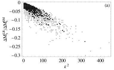
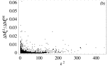
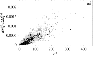
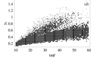
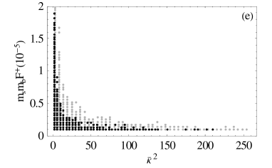
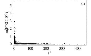
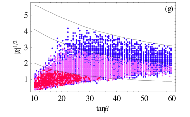
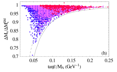
Figure 3: Study of Higgs-mediated contributions to $\Delta M_{q}$ (see text). Black dots denote the points in parameter space that satisfy all constraints, while grey dots refer to those that only satisfy the initial constraints (see Table 3). In plots (g) and (h), blue/magenta/red (dark grey / light grey / grey) points correspond to $M_{A}=550/350/150\ \,\mbox{GeV}$, respectively. Plain lines indicate the $\mathcal{B}(B_{s}\rightarrow\mu^{+}\mu^{-})$ constraint. In plot (h), the dashed line corresponds to the more stringent $\mathcal{B}(B_{s}\rightarrow\mu^{+}\mu^{-})$ constraint in the right column of Table 3.

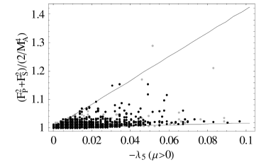
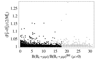
Figure 4: Correction factor to $\mathcal{B}(B_{q}\to\mu^{+}\mu^{-})$ arising from supersymmetric loop effects in the Higgs self-energies as a function of the effective coupling $\lambda_{5}$ (left) and the total Higgs-mediated effects in $B_{s}\to\mu^{+}\mu^{-}$ (right), for $\mu>0$. On the left-hand side, the upper (lower) line corresponds to $M_{A}=120\ (600)\ \,\mbox{GeV}$, assuming the approximate formula of Eq. (93) for the correction factor.

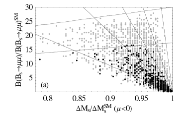
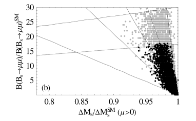
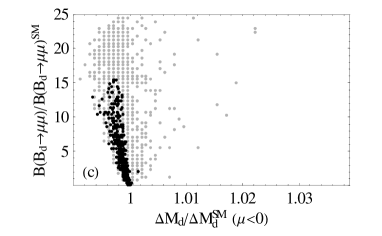
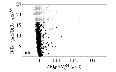
Figure 5: Correlation between $\Delta M_{q}$ and $\mathcal{B}(B_{q}\to\mu^{+}\mu^{-})$: (a) $q=s$, $\mu<0$; (b) $q=s$, $\mu>0$; (c) $q=d$, $\mu<0$; (d) $q=d$, $\mu>0$. The descending lines correspond to a fixed value of the ratio $\tan\beta/M_{A}$. From left to right: $\tan\beta/M_{A}=0.05,0.075,0.10,0.13,0.21\ \,\mbox{GeV}^{-1}$. The ascending lines refer to the $\mathcal{B}(B_{s}\rightarrow\mu^{+}\mu^{-})/\Delta M_{s}$ constraints, see Table 3. These lines do not take into account the uncertainties on the quark masses and bag factors, nor the effects from sparticle loop corrections to the Higgs potential in $\Delta M_{s}$, $\mathcal{B}(B_{s}\rightarrow\mu^{+}\mu^{-})$, and to the lepton Yukawa couplings in $\mathcal{B}(B_{s}\rightarrow\mu^{+}\mu^{-})$, so that the actual points do not follow them exactly but are somewhat scattered.

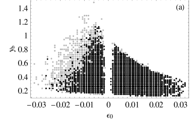
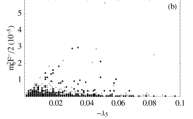
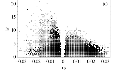
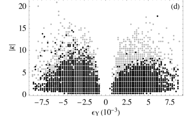
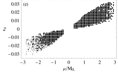
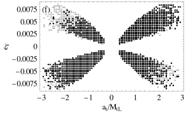
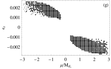
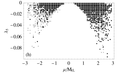
Figure 6: Dependence of various quantities on effective couplings or supersymmetric parameters.

4.3 CP-violating effects

The Higgs-mediated $B\!-\!\,\overline{\!B}{}\,$ mixing amplitudes studied here can in principle generate new contributions to the CP-violating phases measured in the $B_{d}\to J/\psi K_{S}$ time-dependent CP asymmetry and the $B_{s}\to J/\psi\phi$ time-dependent angular distribution. The coefficients of the $\sin(\Delta M_{q}\,t)$ terms are

$$\begin{split}S_{J/\psi K_{S}}=&\sin(2\beta+\phi_{d}^{\Delta}),\\ S_{J/\psi\phi}=&-\sin(-2\beta_{s}+\phi_{s}^{\Delta}),\end{split}$$ (96)

where $\beta\equiv\arg[-(V_{td}^{*}V_{tb})/(V_{cd}^{*}V_{cb})]$, $\beta_{s}\equiv-\arg[-(V_{ts}^{*}V_{tb})/(V_{cs}^{*}V_{cb})]$, and

$$\phi_{q}^{\Delta}=\arg(M_{12}^{q}/M_{12}^{q,\rm SM})\equiv\arg(1+h_{q}).$$ (97)

In $B_{s}\to J/\psi\phi$ an angular analysis separates the different CP components, the sign quoted for $S_{J/\psi\phi}$ in Eq. (96) refers to the dominant CP-even component. These phases have received a lot of attention recently. In particular, the new measurements of $-2\beta_{s}+\phi_{s}^{\Delta}$ by the CDF and D0 collaborations [54], both more than 1.5 sigma above its SM prediction [55], have triggered speculations about the validity of the SM [56]. A possible tension between the value of $\sin 2\beta$ obtained from $S_{J/\psi K_{S}}$ and the amount of CP violation in the kaon system was also pointed out [57].

Looking back at Eqs. (17-19), it is clear that the new phases $\phi_{q}^{\Delta}$, when associated with the $Q^{\rm LR}_{2}$ effective operator, have to be brought up by the quark-Higgs couplings $\kappa_{ij}$ as $\mathcal{F}^{+}$ cannot develop an imaginary part. When associated with $Q^{\rm SLL}_{1}$ or $Q^{\rm SRR}_{1}$, on the other hand, they can arise from both the Yukawa sector and the Higgs potential via $\mathcal{F}^{-}$. Within MFV, $\kappa_{qb}^{\ast}\,\kappa_{bq}=|\bar{\kappa}|^{2}\lambda^{2}_{qb}m_{q}m_{b}/v^{2}$ and only $C^{\rm SLL}_{1}$ can produce a new phase (via $\epsilon_{0,Y}$ or $\lambda_{5,7}$). However, the $B_{s}\rightarrow\mu^{+}\mu^{-}$ branching fraction is barely affected by CP-violating effects, so that its constraints on $|\bar{\kappa}|$ are still very well approximated by the plain lines in Fig. 3(g) (for some representative $M_{A}$ values). As a result, just like in the CP-conserving case, the net effect of the suppression of $|\bar{\kappa}|$ and enhancement of $\mathcal{F}^{-}$ for small $M_{A}$ is quite small. The MSSM with large $\tan\beta$ and MFV is thus not able to account for a large non-standard phase in $B_{s}\!-\!\,\overline{\!B}{}_{s}\,$ (or $B_{d}\!-\!\,\overline{\!B}{}_{d}\,$) mixing, if the evidence for such a phase were confirmed. Let us emphasize, however, that the formulation of MFV adopted here does not coincide exactly with the full symmetry-based definition of Ref. [13]. In the formalism of Ref. [13], it was shown recently that new phases could appear in the $\delta_{LL}^{13,23}$ sector, in addition to those in the $(\delta_{LR}^{d})^{13,23}$ sector [16]. The possible impact of these MFV phases via $\kappa_{qb}^{\ast}\,\kappa_{bq}$ in $C^{\rm LR}_{2}$ is a priori rather limited due to the $B_{s}\rightarrow\mu^{+}\mu^{-}$ constraint, yet a more quantitative analysis is desirable.

Beyond MFV, the $Q^{\rm LR}_{2}$ contribution is expected to dominate. As said before, supersymmetric loop corrections to the Higgs propagator $\mathcal{F}^{+}$ do not bring in any new phases. These can only enter via the quark-Higgs couplings $\kappa_{qb}^{\ast}$ and $\kappa_{bq}$. The possible size of CP-violating effects generated in this way without violating the existing constraints deserves a study on its own. We will not discuss this further here.

5 Conclusions

We have studied supersymmetric loop corrections to the MSSM Higgs sector. While the tree-level Higgs sector of the MSSM is a 2HDM of type II, the soft supersymmetry-breaking terms lead to new loop-induced couplings which result in a generic 2HDM with FCNC couplings of neutral Higgs bosons to quarks, even if the supersymmetry-breaking sector is minimally flavour-violating. The strength of these couplings grows with $\tan\beta$ and precision observables of flavour physics are known to severely constrain large-$\tan\beta$ scenarios of the MSSM. The appropriate tool for such studies is an effective Lagrangian, which is derived by integrating out the heavy supersymmetric particles. The abundant literature on the subject has primarily focused on the flavour-changing Yukawa couplings [1, 2, 3, 4, 5, 6, 7]. Among the FCNC quantities, $B\!-\!\,\overline{\!B}{}\,$ mixing plays a special role, because the apparently dominant contribution of Fig. 1 vanishes. Therefore $B\!-\!\,\overline{\!B}{}\,$ mixing is sensitive to subleading effects, whose systematic study was the main motivation for this paper. Pursuing this goal we have derived several conceptual and analytic results which can be applied well beyond this topic. They can be classified into three categories:

1. MSSM Higgs sector
We have matched the complete MSSM Higgs sector, i.e. both the Yukawa interactions and the Higgs potential, onto an effective 2HDM. Our results for the effective Yukawa couplings are valid for arbitrary CP phases of $\mu$, $a_{t}$, and the gaugino masses; and Eqs. (31) and (32) correct the gaugino contributions to $\epsilon_{0}$ and $\epsilon_{Y}$ quoted in Ref. [25]. The complete one-loop matching corrections for the quartic Higgs couplings for the most general MSSM are explicitly listed in one place for the first time. This result goes beyond minimal flavour violation and beyond the large-$\tan\beta$ limit. It is well-known that improper choices of the MSSM renormalization scheme can lead to radiative corrections which grow with $\tan\beta$ rendering perturbative results unreliable [29]. At the heart of this problem is the feature that $\tan\beta$ is an ill-defined parameter in the general 2HDM, which permits arbitrary rotations among the two Higgs doublets. In the matching of the MSSM onto the 2HDM this feature enters through the wave function renormalization, and we propose an $\overline{\textrm{MS}}$ renormalization of $\tan\beta$ in the 2HDM which is stable in the limit of large $\tan\beta$. The relation to a $\overline{\textrm{DR}}$-renormalized $\tan\beta$ in the MSSM is discussed including electroweak corrections. We identify the places in the effective Higgs potential where physical $\tan\beta$-enhanced effects occur. The coefficients $\lambda_{2}$, $\lambda_{5}$ and $\lambda_{7}$, which are important for $B\!-\!\,\overline{\!B}{}\,$ mixing, are explicitly specified for the MFV case in Eqs. (39–37). Some loop corrections to the Higgs potential at large $\tan\beta$ and their impact on $\tan\beta$ itself and the Higgs-fermion couplings have also been considered in an effective-field-theory framework in Ref. [58], which appeared during completion of this paper. Part of the results therein overlap with Section 3 of this paper. We disagree with [58] in some points (cf. Section 3), notably in that we find a $\tan\beta$-enhanced term in the relation of the $\overline{DR}$ and DCPR $\tan\beta$ parameters. We stress that, in general, only the former is numerically close to the $\tan\beta$ parameter extracted from $B$-physics observables.

2. Large $\mathit{\tan\beta}$ phenomenology
The prime application of our results is $B\!-\!\,\overline{\!B}{}\,$ mixing. We have identified a global $U(1)$ symmetry of the $\bar{b}_{R}q_{L}$ Higgs-mediated FCNC transitions and the tree-level Higgs potential in the large-$\tan\beta$ limit which suppresses the superficially leading contribution of Fig. 1. A systematic study of $B\!-\!\,\overline{\!B}{}\,$ mixing has required the analyses of four subleading contributions, which are governed by the small parameters $m_{d,s}/m_{b}$, $1/\tan\beta$, $v/M_{\rm SUSY}$ and the loop factor $1/(4\pi)^{2}$. These parameters either provide a breaking of the $U(1)$ symmetry or allow for a contribution proportional to the $U(1)$-conserving standard-model effective operator. Prior to this work, only corrections involving $m_{d,s}/m_{b}$ had been studied [5] (with the exception of Ref.[25]). The $v/M_{\rm SUSY}$ corrections are found numerically small. The new loop contributions include all non-decoupling SUSY corrections to the quartic Higgs interactions $\lambda_{1}$–$\lambda_{7}$ and the contribution of neutral Higgs box diagrams in the effective theory. In the complex MSSM the results for ${\cal F}^{\pm}$ comprising the neutral Higgs propagators become cumbersome. We have expressed ${\cal F}^{\pm}$ in terms of sub-determinants of the neutral Higgs mass matrix. These expressions are easy to implement and clearly reveal the invariance of the Higgs-mediated amplitudes under rotations of the basis $(H_{u},-\varepsilon H_{d})$. The results for the Higgs sector are also used to refine the MSSM predictions for the $B^{+}\to\tau^{+}\nu$ and the $B_{s,d}\to\mu^{+}\mu^{-}$ branching ratios. In this context we stress that loop corrections to the Higgs potential do not give rise to additional $\tan\beta$-enhanced contributions to the charged-Higgs-fermion couplings beyond those known before Ref. [25] appeared. Hence no modification of the charged-Higgs contributions to $B^{+}\to\tau^{+}\nu$ or $B\to X_{s}\gamma$ relative to Ref. [5] occurs.

While the MSSM corrections to $B\!-\!\,\overline{\!B}{}\,$ mixing in the large $\tan\beta$ scenario could be dominated by the contribution of $\lambda_{5}$ and $\lambda_{7}$, the size of this piece is limited by the experimental upper bound on ${\cal B}(B_{s}\to\mu^{+}\mu^{-})$. After performing an exhaustive analysis of this quantity, ${\cal B}(\bar{B}\to X_{s}\gamma)$, ${\cal B}(B^{+}\to\tau^{+}\nu)$ and the mass of the lightest neutral Higgs boson $M_{h}$, we find that the impact of the corrections to the Higgs potential on $\Delta M_{s}$ is always weaker than that of the $m_{s}/m_{b}$ correction identified in Ref. [5]. Assessing the total Higgs-mediated MSSM corrections to $\Delta M_{s}$ we find an upper limit of 7% of the SM contribution for $\mu>0$ and $M_{A}<600\,\mbox{GeV}$. If $\mu$ is negative, the upper bound is around 20%. This is in contrast with Refs. [52] and Ref.[25], which claim large effects of the Higgs potential on $B\!-\!\,\overline{\!B}{}\,$ mixing. The corrections to ${\cal B}(B_{q}\to\mu^{+}\mu^{-})$ from the Higgs potential are typically also small, but can reach 15% in some corners of the parameter space. In summary, the correlation between an enhancement of ${\cal B}(B_{q}\to\mu^{+}\mu^{-})$ and a (moderate) depletion of $\Delta M_{s}$ found in Ref. [5] remains essentially intact.

We finally note that our new contributions can alter the CP phase of the $B\!-\!\,\overline{\!B}{}\,$ mixing amplitude, while the previously known Higgs contribution proportional to $m_{s}m_{b}{\cal F}^{+}$ has the same phase as the SM term (in MFV scenarios). While the maximal possible CP phase is clearly below the sensitivity of the current Tevatron experiments, it is an open question whether future $B\!-\!\,\overline{\!B}{}\,$ mixing experiments can help to unravel the CP structure of the MSSM Higgs potential.

3. Heavy-quark relations and bag parameters
We have transformed the NLO anomalous dimensions computed in Ref.[26] to an operator basis and a renormalization scheme typically used in lattice calculations. The according anomalous dimensions are needed to evaluate the ‘bag’ parameters, which parametrise the hadronic matrix elements, at the electroweak scale. We further employed a heavy-quark relation to improve the numerical prediction of the bag parameter $B_{1}^{\textrm{SLL}\,\prime}$ entering the SUSY contributions to $B\!-\!\,\overline{\!B}{}\,$ mixing. The heavy-quark relation essentially determines $B_{1}^{\textrm{SLL}\,\prime}$ in terms of the bag parameter $B_{1}^{\rm VLL}$, which is needed for the SM prediction [55]. We found $P^{\rm SLL}_{1}=-\frac{5}{8}B_{1}^{\rm SLL\,\prime}(m_{t})=-1.36\pm 0.12$.

Appendix A Notations and conventions

To state our phase conventions for $\mu$ and $M_{2}$ we quote the chargino mass matrix:

$${\cal M}_{\chi^{+}}=\left(\begin{array}[]{cc}\displaystyle M_{2}&\displaystyle\frac{g\ v\sin\beta}{\sqrt{2}}\\ \displaystyle\frac{g\ v\cos\beta}{\sqrt{2}}&\displaystyle\mu\end{array}\right)$$ (98)

with $v=246\,\mbox{GeV}$ and the chargino mass term in the Lagrangian

$${\cal L}_{\chi^{+}}^{\rm mass}=-(\lambda^{-},\widetilde{h}{}_{d}^{2}){\cal M}_{\chi^{+}}(\lambda^{+},\widetilde{h}{}_{u}^{1})^{T}\,.$$ (99)

For the case of a general flavour structure of the squark mass matrices we define the trilinear couplings $\hat{T}_{u_{ij}}$ and $\hat{T}_{d_{ij}}$ (with flavour indices $i,j$) such that the squark mass matrices read

$$\hat{\cal M}^{2}_{\widetilde{u}} = \left(\begin{array}[]{cc}\displaystyle\hat{M}^{2}_{\widetilde{u}_{L}}&\displaystyle\frac{v\sin\beta}{\sqrt{2}}\left[\hat{T}^{\dagger}_{u}-\mu\,\hat{Y}^{\dagger}_{u}\cot\beta\right]\\[5.69054pt] \displaystyle\frac{v\sin\beta}{\sqrt{2}}\left[\hat{T}_{u}-\mu^{*}\hat{Y}_{u}\cot\beta\right]&\displaystyle\hat{M}^{2}_{\widetilde{u}_{R}}\end{array}\right),$$ (102)

$$\hat{\cal M}^{2}_{\widetilde{d}} = \left(\begin{array}[]{cc}\displaystyle\hat{M}^{2}_{\widetilde{d}_{L}}&\displaystyle\frac{v\cos\beta}{\sqrt{2}}\left[\hat{T}^{\dagger}_{d}-\mu\,\hat{Y}^{\dagger}_{d}\tan\beta\right]\\[5.69054pt] \displaystyle\frac{v\cos\beta}{\sqrt{2}}\left[\hat{T}_{d}-\mu^{*}\hat{Y}_{d}\tan\beta\right]&\displaystyle\hat{M}^{2}_{\widetilde{d}_{R}}\end{array}\right),$$ (105)

in the super-CKM basis, where the ($\overline{\rm DR}$-renormalized) Yukawa matrices are diagonal: $\hat{Y}_{q}=\mbox{diag}\,(y_{q_{1}},y_{q_{2}},y_{q_{3}})$, $q=u,d$. The mass matrices in Eq. (105) correspond to the squark mass term

$${\cal L}^{\rm mass}_{\widetilde{q}}=-\Phi^{\dagger}_{\widetilde{u}}\hat{\cal M}^{2}_{\widetilde{u}}\Phi_{\widetilde{u}}-\Phi^{\dagger}_{\widetilde{d}}\hat{\cal M}^{2}_{\widetilde{d}}\Phi_{\widetilde{d}}$$ (106)

with $\Phi_{\widetilde{u}}=(\widetilde{u}_{L},\widetilde{c}_{L},\widetilde{t}_{L},\widetilde{u}_{R},\widetilde{c}_{R},\widetilde{t}_{R})^{T}$ and $\Phi_{\widetilde{d}}=(\widetilde{d}_{L},\widetilde{s}_{L},\widetilde{b}_{L},\widetilde{d}_{R},\widetilde{s}_{R},\widetilde{b}_{R})^{T}$.

Our sign convention for the MSSM Yukawa couplings implies the following relations between 2HDM quark masses and MSSM Yukawa couplings in the up sector:

$$y_{u_{i}} = \frac{\sqrt{2}}{v\sin\beta}\,m_{u_{i}}.$$ (107)

In general, the analogous relations in the down sector involve complex phases associated with the $\tan\beta$-enhanced threshold corrections in Eq. (22). In particular, Ref. [24], which discusses the complex MSSM for the case without flavor mixing, relates the $b$ Yukawa coupling to the $b$ quark mass as

$$y_{b} = \frac{\sqrt{2}}{v\cos\beta}\,\frac{m_{b}}{1+\widetilde{\epsilon}_{3}\tan\beta},$$ (108)

rendering $y_{b}$ complex for complex $\widetilde{\epsilon}_{3}$ in Eq. (33). Our approach of matching the MSSM to an effective 2HDM permits different phase conventions, because the quark fields in the MSSM and the 2HDM can be chosen to differ by a phase factor. We can rephase the $b_{R}$ super-field of the MSSM in such a way that $y_{b}$ is real and positive and $1+\widetilde{\epsilon}_{3}\tan\beta$ in Eq. (108) is replaced by $|1+\widetilde{\epsilon}_{3}\tan\beta|$. The (physical) phase of $1+\widetilde{\epsilon}_{3}\tan\beta$ will then, however, appear explicitly in the Higgs and higgsino couplings to bottom (s)quarks. Introducing $3\times 3$ flavour mixing, the relation between $\hat{Y}_{d}$ and $m_{d}$, $m_{s}$, $m_{b}$ is found from Eq. (22). Now the quark fields in the 2HDM differ from those in the MSSM by a complex rotation in flavour space and a particular choice for the phases of MSSM fields appears less obvious. In particular, one could render all $y_{d_{i}}$ real and positive by suitable rephasings of the right-handed superfields. Note that within MFV $y_{b}$ is still related to $m_{b}$ via Eq. (108) in good approximation without such rephasings. The analogous relation for the first two generations reads

$$y_{d,s} = \frac{\sqrt{2}}{v\cos\beta}\,\frac{m_{d,s}}{1+\epsilon_{0}\tan\beta}\,,$$ (109)

while in the lepton sector, we have

$$y_{\ell} = \frac{\sqrt{2}}{v\cos\beta}\,\frac{m_{\ell}}{1+\epsilon_{\ell}\tan\beta}\qquad\qquad\mbox{with $\ell=e,\mu,\tau$}\,.$$ (110)

In (most of) the paper we express our results in terms of fermion masses (i.e. avoiding $y_{d_{i},\ell}$) to achieve formulae which are independent of such phase conventions. Note that the phases of $\epsilon_{0}$ and $\epsilon_{Y}$ are physical and no phase convention other than that of the CKM matrix matters for $\kappa_{ij}$ in Eqs. (29) and (30). While the phase convention of $y_{q_{i}}$ enters the phases in $\hat{T}_{q}$, it drops out from the MFV parameters $a_{q}$ in Eq. (114).

Finally, the quadratic squark soft-breaking terms are defined as follows:

$$\begin{split}(\hat{M}^{2}_{\widetilde{u}_{L}})_{ij}=&\ (V_{CKM}^{0}\,\tilde{m}^{2}_{Q}V_{CKM}^{0\dagger})_{ij}+\frac{v^{2}\sin^{2}\beta}{2}\delta_{ij}|y_{u_{i}}|^{2}+\delta_{ij}M^{2}_{Z}\cos 2\beta(1/2-2\sin^{2}\theta_{W}/3),\\ (\hat{M}^{2}_{\widetilde{d}_{L}})_{ij}=&\ (\tilde{m}^{2}_{Q})_{ij}+\frac{v^{2}\cos^{2}\beta}{2}\delta_{ij}|y_{d_{i}}|^{2}+\delta_{ij}M^{2}_{Z}\cos 2\beta(-1/2+\sin^{2}\theta_{W}/3),\\ (\hat{M}^{2}_{\widetilde{u}_{R}})_{ij}=&\ (\tilde{m}^{2}_{u})_{ij}+\frac{v^{2}\sin^{2}\beta}{2}\delta_{ij}|y_{u_{i}}|^{2}+2\delta_{ij}M^{2}_{Z}\cos 2\beta\sin^{2}\theta_{W}/3,\\ (\hat{M}^{2}_{\widetilde{d}_{R}})_{ij}=&\ (\tilde{m}^{2}_{d})_{ij}+\frac{v^{2}\cos^{2}\beta}{2}\delta_{ij}|y_{d_{i}}|^{2}-\delta_{ij}M^{2}_{Z}\cos 2\beta\sin^{2}\theta_{W}/3\,,\end{split}$$ (111)

where $V_{CKM}^{0}$ corresponds to the relative rotation of left-handed $u$-type and $d$-type quark fields performed when diagonalizing the Yukawa matrices. It differs from the actual CKM matrix, defined by the rotations that diagonalize the 2HDM mass matrices rather than the MSSM Yukawa couplings, by loop-suppressed (but $\tan\beta$-enhanced) corrections. In particular, within MFV, we have:

$$V_{CKM_{ij}}=\begin{cases}\Big{|}\frac{\displaystyle 1+\epsilon_{0}\tan\beta}{\displaystyle 1+\widetilde{\epsilon}_{3}\tan\beta}\ \Big{|}V^{0}_{CKM_{ij}}&{\rm for}\ (i,j)=(u,b),(c,b),(t,d),(t,s),\\[8.53581pt] V^{0}_{CKM_{ij}}&{\rm otherwise}.\end{cases}$$ (112)

The relations Eq. (112) take a particularly compact form in the (exact) Wolfenstein parametrization, where one has

$$A=\Big{|}\frac{\displaystyle 1+\epsilon_{0}\tan\beta}{\displaystyle 1+\widetilde{\epsilon}_{3}\tan\beta}\ \Big{|}A^{0},\quad\lambda=\lambda^{0},\quad\bar{\rho}=\bar{\rho}^{0},\quad\bar{\eta}=\bar{\eta}^{0}.$$ (113)

Whenever we consider the case of MFV we write

$$\hat{T}_{u_{ij}}=a_{t}y_{u_{i}}\delta_{ij},\quad\hat{T}_{d_{ij}}=a_{b}y_{d_{i}}\delta_{ij},\quad\tilde{m}^{2}_{Q_{ij}}=\tilde{m}^{2}_{Q}\delta_{ij},\quad\tilde{m}^{2}_{u_{ij}}=\tilde{m}^{2}_{u}\delta_{ij},\quad\tilde{m}^{2}_{d_{ij}}=\tilde{m}^{2}_{d}\delta_{ij}.$$ (114)

The SU(2) relation between $\hat{M}^{2}_{\widetilde{d}_{L}}$ and $\hat{M}^{2}_{\widetilde{u}_{L}}$ then implies for the third generation:

$$M^{2}_{\widetilde{t}_{L}}\;=\;M^{2}_{\widetilde{b}_{L}}\,+\,m_{t}^{2}\,-\,\frac{m_{b}^{2}}{|1+\widetilde{\epsilon}_{3}\tan\beta|^{2}}\,+\,M^{2}_{Z}\cos 2\beta(1-\sin^{2}\theta_{W}).$$ (115)

In the strict SU(2) limit (i.e., $v/M_{\rm SUSY}\to 0$) one has $M^{2}_{\widetilde{t}_{L}}\;=\;M^{2}_{\widetilde{b}_{L}}$, but for small $M^{2}_{\widetilde{b}_{L}}$ the term involving $m_{t}^{2}$ can be relevant. Also FCNC $\widetilde{W}$-$\widetilde{u}_{Li}$ loops vanish (for universal $M^{2}_{\widetilde{u}_{L}}$) by the GIM mechanism up to the $m_{t}^{2}$ term in Eq. (115).

Finally, it is convenient to define the so-called superflavour basis, obtained from a generic electroweak interaction eigenstate basis by rotating the supermultiplets $Q_{L}$, $u_{R}$ and $d_{R}$ such that the quadratic squark soft-breaking terms are diagonal. We denote the corresponding entries by $\tilde{m}^{2}_{Q_{i}}$, $\tilde{m}^{2}_{u_{i}}$, and $\tilde{m}^{2}_{d_{i}}$. For $M_{\rm SUSY}\gg v$, these are just the squark masses, and the computation of the effective couplings $\lambda_{i}$ induced by heavy squark loops for arbitrary flavour and CP structure is greatly simplified. The Yukawa matrices and trilinear terms in this basis are simply written $Y_{u,d}$ and $T_{u,d}$, respectively. They are given in terms of $\hat{Y}_{u,d}$ and $\hat{T}_{u,d}$ as follows:

$$Y_{u}^{T}=U_{u}\hat{Y}_{u}V_{CKM}^{0}V_{d}^{\dagger},\quad Y_{d}^{T}=U_{d}\hat{Y}_{d}V_{d}^{\dagger},\quad T_{u}^{T}=U_{u}\hat{T}_{u}V_{CKM}^{0}V_{d}^{\dagger},\quad T_{d}^{T}=U_{d}\hat{T}_{d}V_{d}^{\dagger},$$ (116)

where the matrices $V_{d}$, $U_{u}$ and $U_{d}$ are defined such that

$$\textrm{diag}(\tilde{m}^{2}_{Q_{i}})=V_{d}\tilde{m}^{2}_{Q}V_{d}^{\dagger},\quad\textrm{diag}(\tilde{m}^{2}_{u_{i}})=U_{u}\tilde{m}^{2}_{u}U_{u}^{\dagger},\quad\textrm{diag}(\tilde{m}^{2}_{d_{i}})=U_{d}\tilde{m}^{2}_{d}U_{d}^{\dagger}.$$ (117)

Assuming MFV, one is allowed to choose $V_{d}=U_{u}=U_{d}=1$.

Our conventions comply with the Les Houches accord [59]. In particular, our $Y_{u,d}$ and $T_{u,d}$ matrices correspond to a particular choice of the generic $Y_{u,d}$ and $T_{u,d}$ matrices of Ref.[59]. Our conventions also agree with those of Ref. [60], except that the sign convention of our $\hat{Y}_{d}$ in Eq. (108) is opposite. Besides, our $\hat{T}_{u}$ equals $-A_{u}$ and our $\hat{T}_{d}$ equals $A_{d}$ of Ref. [60], respectively.

Appendix B Matching of the MSSM on a 2HDM

The notation of Sect. 3 distinguishes between the coefficients $\hat{\lambda}_{i}$ and $\bar{\lambda}_{i}$. The former quantities contain the results from the supersymmetric loop corrections to the quadrilinear Higgs couplings, whose tree-level values are given in Eq. (21). The latter coefficients also include the effect of the wave function and gauge coupling renormalization constants in Sect. B.1.

In the following we summarize the one-loop matching corrections for the quartic Higgs-coupling constants in the general MSSM. While the calculation of loop corrections to the Higgs sector of the MSSM has a long history, see for example [18, 19, 20, 21, 23, 22, 24], and a determined reader could extract part of the matching coefficients below from these works, the results collected in this appendix as a service to the reader are more complete than those in the literature, capturing the effects of the full set of mass, flavour-violation, and CP-violation parameters of the most general MSSM.

The general results are quite lengthy hence we start with $\bar{\lambda}_{2,5,7}$, where all renormalization constants are included, in the approximation of third generation dominance and degenerate soft-breaking parameters $\tilde{m}^{2}_{u,d,Q,e,l}=\tilde{m}^{2}$ and $M_{1,2}=M_{1/2}$. The quartic coupling constant $\lambda_{2}$ is already present at tree level and as such depends on the renormalization scale $\mu_{0}$ at one-loop. It reads:

$$\begin{split}\bar{\lambda}_{2}=&\frac{\tilde{g}^{2}}{4}+\frac{1}{16\pi^{2}}\Bigg{\{}-\frac{\frac{1}{2}\left|a_{t}y_{t}\right|{}^{4}+\frac{1}{2}|\mu|^{4}\left|y_{b}\right|{}^{4}+\frac{1}{6}|\mu|^{4}\left|y_{\tau}\right|{}^{4}}{\tilde{m}^{4}}\\ &\qquad+\frac{\left(6\left|y_{t}\right|{}^{2}-\frac{1}{2}\tilde{g}^{2}\right)\left|a_{t}y_{t}\right|{}^{2}+\tilde{g}^{2}|\mu|^{2}\left|y_{b}\right|{}^{2}+\frac{1}{3}\tilde{g}^{2}|\mu|^{2}\left|y_{\tau}\right|{}^{2}}{\tilde{m}^{2}}\\ &\qquad+\left(g^{4}-\frac{3}{2}\left|y_{t}\right|{}^{2}g^{2}+\frac{5g^{\prime^{4}}}{3}+6\left|y_{t}\right|{}^{4}-\frac{3}{2}g^{\prime^{2}}\left|y_{t}\right|{}^{2}\right)\log\left(\frac{\tilde{m}^{2}}{\mu_{0}^{2}}\right)\\ &\qquad+g^{4}\left(\frac{\log\left(M_{\mu}\right)\left(13-3M_{\mu}\right)M_{\mu}^{2}}{4\left(M_{\mu}-1\right){}^{3}}-\frac{11}{12}\log\left(\frac{|\mu|^{2}}{\mu_{0}^{2}}\right)-\frac{M_{\mu}\left(5M_{\mu}+14\right)+1}{8\left(M_{\mu}-1\right){}^{2}}\right)\\ &\qquad+g^{2}\,g^{\prime^{2}}\left(-\frac{2\log\left(M_{\mu}\right)\left(M_{\mu}-4\right)M_{\mu}^{2}}{\left(M_{\mu}-1\right){}^{3}}-\frac{\left(M_{\mu}+5\right)M_{\mu}}{\left(M_{\mu}-1\right){}^{2}}-2\log\left(\frac{|\mu|^{2}}{\mu_{0}^{2}}\right)\right)\\ &\qquad+g^{\prime^{4}}\left(-\frac{15}{4}\log\left(\frac{|\mu|^{2}}{\mu_{0}^{2}}\right)-\frac{M_{\mu}\left(17M_{\mu}+158\right)+5}{24\left(M_{\mu}-1\right){}^{2}}+\right.\\ &\qquad\qquad\left.\frac{\log\left(M_{\mu}\right)\left(M_{\mu}\left(\left(141-43M_{\mu}\right)M_{\mu}-12\right)+4\right)}{12\left(M_{\mu}-1\right){}^{3}}\right)\Bigg{\}}\,,\end{split}$$ (118)

where we have defined the mass ratio $M_{\mu}=|M|^{2}_{1/2}/|\mu|^{2}$. Its renormalization-scale dependence is cancelled by the inclusion of electroweak corrections in the effective 2HDM. The other coupling constants important in the large $\tan\beta$ limit are

$$\begin{split}\bar{\lambda}_{5}=\frac{1}{16\pi^{2}}&\Bigg{\{}-\frac{\mu^{2}\left(3a_{b}^{2}\left|y_{b}\right|{}^{4}+3\left|y_{t}\right|{}^{4}a_{t}^{2}+\left|y_{\tau}\right|{}^{4}a_{\tau}^{2}\right)}{6\tilde{m}^{4}}\\ &\qquad+\frac{\left(g^{4}+2g^{\prime^{2}}g^{2}+3g^{\prime^{4}}\right)\left(\log\left(M_{\mu}\right)+\left(\log\left(M_{\mu}\right)-2\right)M_{\mu}+2\right)}{\left(M_{\mu}-1\right){}^{3}}\Bigg{\}}\end{split}$$ (119)

and

$$\begin{split}\bar{\lambda}_{7}=\frac{1}{16\pi^{2}}&\Bigg{\{}\frac{1}{\tilde{m}^{2}}\left(-3\mu a_{t}\left|y_{t}\right|^{4}-\frac{1}{12}\mu\tilde{g}^{2}\left(6a_{b}\left|y_{b}\right|^{2}-3\left|y_{t}\right|^{2}a_{t}+2\left|y_{\tau}\right|^{2}a_{\tau}\right)\right)\\ &+\frac{\mu}{6\tilde{m}^{4}}\left(3\left|a_{t}\right|^{2}a_{t}\left|y_{t}\right|^{4}+|\mu|^{2}\left(3a_{b}\left|y_{b}\right|^{4}+\left|y_{\tau}\right|^{4}a_{\tau}\right)\right)\\ &+\left(\left(g^{4}+4g^{\prime^{2}}g^{2}+3g^{\prime^{4}}\right)\frac{\mu}{|\mu|}+8\left(g^{4}+2g^{\prime^{2}}g^{2}+3g^{\prime^{4}}\right)\frac{M_{1/2}}{\mu^{*}}\right)\times\\ &\qquad\frac{\left(-M_{\mu}^{2}+2\log\left(M_{\mu}\right)M_{\mu}+1\right)}{8\left(M_{\mu}-1\right){}^{3}}\Bigg{\}}\,.\end{split}$$ (120)

In the following subsections we quote the results for $\hat{\lambda}_{i}$ in the general MSSM. The effective potential $V$ in Eq. (12) must be used with $\lambda_{i}=\bar{\lambda}_{i}$ and the relation between $\bar{\lambda}_{i}$ and $\hat{\lambda}_{i}$ is given in Eq. (3.1); the renormalization constants needed in this relation are given in Sect. B.1. We decompose $\hat{\lambda}_{1-7}$ as

$$\begin{split}\hat{\lambda}_{i}=&\lambda_{i}^{\rm tree}\,+\,\frac{\lambda_{i}^{\rm ino}+\lambda_{i}^{\rm sferm}}{16\pi^{2}}.\end{split}$$ (121)

The tree-level values $\lambda_{i}^{\rm tree}$ are given in Eq. (21). $\lambda_{i}^{\rm ino}$ and $\lambda_{i}^{\rm sferm}$, given in Sect. B.2 and B.3, contain the contributions from higgsino and gaugino loops and from sfermion loops, respectively. Finally we also list the relevant loop functions in Sect. B.4. All these results are given in the superflavour basis including the most general soft-breaking terms.

B.1 Renormalization constants

The renormalization of $g^{(\prime)}$ is related only to the field renormalization of $W$ and $B$, $Z_{W,B}=1+\delta Z_{W,B}$, if we decouple the sfermionic, higgsino and gaugino contributions: $\delta g^{\prime}=-\delta Z_{B}/2$ and $\delta g=-\delta Z_{W}/2$. The finite part of the one-loop wavefunction renormalization constants of the gauge bosons are

$$\begin{split}\delta Z_{W}&=\frac{g^{2}}{16\pi^{2}}\frac{1}{6}\left[4\log\frac{|\mu|^{2}}{\mu_{0}^{2}}+8\log\frac{M_{2}^{2}}{\mu_{0}^{2}}+\sum_{i=1}^{3}\left(\log\frac{\tilde{m}_{l_{i}}^{2}}{\mu_{0}^{2}}+N_{C}\log\frac{\tilde{m}_{Q_{i}}^{2}}{\mu_{0}^{2}}\right)-4\right]\\ \delta Z_{B}&=\frac{g^{\prime^{2}}}{16\pi^{2}}\frac{1}{3}\left[2\log\frac{|\mu|^{2}}{\mu_{0}^{2}}+\sum_{i=1}^{3}\left(\log\frac{\tilde{m}_{e_{i}}^{2}}{\mu_{0}^{2}}+\frac{1}{2}\log\frac{\tilde{m}_{l_{i}}^{2}}{\mu_{0}^{2}}+\right.\right.\\ &\qquad\qquad\qquad\qquad\qquad\left.\left.\frac{4N_{C}}{9}\log\frac{\tilde{m}_{u_{i}}^{2}}{\mu_{0}^{2}}+\frac{N_{C}}{9}\log\frac{\tilde{m}_{d_{i}}^{2}}{\mu_{0}^{2}}+\frac{N_{C}}{18}\log\frac{\tilde{m}_{Q_{i}}^{2}}{\mu_{0}^{2}}\right)\right]\,,\end{split}$$ (122)

where $\mu_{0}$ is the renormalization scale and the soft-breaking terms are written in the superflavour basis (see Appendix A).

The sfermionic contributions to the wavefunction renormalization constants of the Higgs bosons are

$$\begin{split}\delta Z_{dd}&={\frac{1}{32\pi^{2}}}\sum_{ij}\left[3B_{0}^{\prime}\left(\tilde{m}_{d_{i}},\tilde{m}_{Q_{j}}\right){T_{d_{ji}}}{T_{d_{ji}}^{*}}+3|\mu|^{2}B_{0}^{\prime}\left(\tilde{m}_{u_{i}},\tilde{m}_{Q_{j}}\right)Y_{u_{ji}}Y_{u_{ji}}^{*}\right.\\ &\qquad\qquad\qquad\qquad\qquad\qquad+\left.B_{0}^{\prime}\left(\tilde{m}_{e_{i}},\tilde{m}_{l_{j}}\right){T_{e_{ji}}}{T_{e_{ji}}^{*}}\right]\\ \delta Z_{ud}&={-\frac{1}{16\pi^{2}}}\sum_{ij}\left[3\mu^{*}B_{0}^{\prime}\left(\tilde{m}_{d_{i}},\tilde{m}_{Q_{j}}\right){T_{d_{ji}}^{*}}Y_{d_{ji}}+3\mu^{*}B_{0}^{\prime}\left(\tilde{m}_{u_{i}},\tilde{m}_{Q_{j}}\right){T_{u_{ji}}^{*}}Y_{u_{ji}}\right.\\ &\qquad\qquad\qquad\qquad\qquad\qquad+\left.\mu^{*}B_{0}^{\prime}\left(\tilde{m}_{e_{i}},\tilde{m}_{l_{j}}\right){T_{e_{ji}}^{*}}Y_{e_{ji}}\right]\\ \delta Z_{uu}&={\frac{1}{32\pi^{2}}}\sum_{ij}\left[3B_{0}^{\prime}\left(\tilde{m}_{u_{i}},\tilde{m}_{Q_{j}}\right){T_{u_{ji}}}{T_{u_{ji}}^{*}}+3|\mu|^{2}B_{0}^{\prime}\left(\tilde{m}_{d_{i}},\tilde{m}_{Q_{j}}\right)Y_{d_{ji}}Y_{d_{ji}}^{*}\right.\\ &\qquad\qquad\qquad\qquad\qquad\qquad+\left.|\mu|^{2}B_{0}^{\prime}\left(\tilde{m}_{e_{i}},\tilde{m}_{l_{j}}\right)Y_{e_{ji}}^{*}Y_{e_{ji}}\right]\,,\end{split}$$ (123)

while the respective contributions of the gaugino and higgsino loops read:

$$\begin{split}\delta Z_{dd}&=-\frac{1}{16\pi^{2}}\frac{1}{8}\left(g^{\prime^{2}}W(|M_{1}|,|\mu|)+3g^{2}W(|M_{2}|,|\mu|)\right)\\ \delta Z_{ud}&=-\frac{1}{16\pi^{2}}\mu^{*}\left(g^{\prime^{2}}M_{1}^{*}B_{0}^{\prime}(|M_{1}|,|\mu|)+3g^{2}M_{2}^{*}B_{0}^{\prime}(|M_{2}|,|\mu|)\right)\\ \delta Z_{uu}&=-\frac{1}{16\pi^{2}}\frac{1}{8}\left(g^{\prime^{2}}W(|M_{1}|,|\mu|)+3g^{2}W(|M_{2}|,|\mu|)\right)\,.\\ \end{split}$$ (124)

B.2 Higgsino-gaugino contributions to $\lambda_{1}$–$\lambda_{7}$

The situation of $\bar{\lambda}_{5}=\hat{\lambda}_{5}$ is particularly simple: The matching correction only involves the box function and $\lambda_{5}^{\rm ino}$ can be written in a compact form:

$$\begin{split}\lambda_{5}^{\rm ino}=&3g^{4}\mu^{2}M_{2}^{2}D_{0}\left(M_{2},M_{2},|\mu|,|\mu|\right)+\\ &2g^{2}g^{\prime^{2}}\mu^{2}M_{1}M_{2}D_{0}\left(M_{1},M_{2},|\mu|,|\mu|\right)+\\ &g^{\prime^{4}}\mu^{2}M_{1}^{2}D_{0}\left(M_{1},M_{1},|\mu|,|\mu|\right)\,,\end{split}$$ (125)

if we use the loop functions defined in Sect. B.4.

We find for $\lambda^{\rm ino}=\lambda_{1}^{\rm ino},\ldots\lambda_{4}^{\rm ino},\lambda_{6}^{\rm ino},\lambda_{7}^{\rm ino}$:

$$\begin{split}\lambda^{\rm ino}=&g^{4}\left(a_{s}+a_{2}\tilde{D}_{2}\left(M_{2},M_{2},|\mu|,|\mu|\right)+a_{4}\tilde{D}_{4}\left(M_{2},M_{2},|\mu|,|\mu|\right)\right)+\\ &g^{2}g^{\prime^{2}}\left(a^{\prime}_{s}+a^{\prime}_{2}\tilde{D}_{2}\left(M_{1},M_{2},|\mu|,|\mu|\right)+a^{\prime}_{4}\tilde{D}_{4}\left(M_{1},M_{2},|\mu|,|\mu|\right)\right)+\\ &g^{\prime^{4}}\left(a^{\prime\prime}_{s}+a^{\prime\prime}_{2}\tilde{D}_{2}\left(M_{1},M_{1},|\mu|,|\mu|\right)+a^{\prime\prime}_{4}\tilde{D}_{4}\left(M_{1},M_{1},|\mu|,|\mu|\right)\right)\,,\end{split}$$ (126)

where the coefficients $a_{s},\ldots a^{\prime\prime}_{4}$ depend on the index $i$ labeling $\lambda_{i}$ in Eq. (121), which we suppress throughout this appendix. The coefficients $a_{2,4}^{(\prime(\prime))}$ are given in Table 4, while

$$a_{s}=\left\{\begin{array}[]{c}-\frac{3}{4}\\ 0\\ 0\end{array}\right.,\quad a_{s}^{\prime}=\left\{\begin{array}[]{c}-\frac{1}{2}\\ 1\\ 0\end{array}\right.,\quad a_{s}^{\prime\prime}=\left\{\begin{array}[]{c}-\frac{1}{4}\\ 0\\ 0\end{array}\right.\quad\textrm{for}\quad\left\{\begin{array}[]{l}\lambda_{1}\;\textrm{to}\;\lambda_{3}\\ \lambda_{4}\\ \lambda_{5}\;\textrm{to}\;\lambda_{7}\end{array}\right.$$ (127)

$\lambda$	$a_{2}$	$a_{4}$	$a^{\prime}_{2}$	$a^{\prime}_{4}$	$a^{\prime\prime}_{2}$	$a^{\prime\prime}_{4}$
$\lambda_{1}$	$\frac{1}{2}|M_{2}|^{2}$	$\frac{5}{2}$	$\frac{1}{2}(M_{1}M_{2}^{*}+M_{1}^{*}M_{2})$	$1$	$\frac{1}{2}|M_{1}|^{2}$	$\frac{1}{2}$
$\lambda_{2}$	$\frac{1}{2}|M_{2}|^{2}$	$\frac{5}{2}$	$\frac{1}{2}(M_{1}M_{2}^{*}+M_{1}^{*}M_{2})$	$1$	$\frac{1}{2}|M_{1}|^{2}$	$\frac{1}{2}$
$\lambda_{3}$	$3|\mu|^{2}+\frac{5}{2}|M_{2}|^{2}$	$\frac{1}{2}$	$2|\mu|^{2}+\frac{1}{2}(M_{1}M_{2}^{*}+M_{1}^{*}M_{2})$	$1$	$|\mu|^{2}+\frac{1}{2}|M_{1}|^{2}$	$\frac{1}{2}$
$\lambda_{4}$	$-3|\mu|^{2}-2|M_{2}|^{2}$	$2$	$2|\mu|^{2}-M_{1}M_{2}^{*}-M_{1}^{*}M_{2}$	$-2$	$-|\mu|^{2}$	$\mathrm{𝟎}$
$\lambda_{6}$	$3\mu M_{2}$	$\mathrm{𝟎}$	$\mu\left(M_{1}+M_{2}\right)$	$\mathrm{𝟎}$	$\mu M_{1}$	$\mathrm{𝟎}$
$\lambda_{7}$	$3\mu M_{2}$	$\mathrm{𝟎}$	$\mu\left(M_{1}+M_{2}\right)$	$\mathrm{𝟎}$	$\mu M_{1}$	$\mathrm{𝟎}$

Table 4: Coefficients entering $\lambda_{1}^{\rm ino}$–$\lambda_{4}^{\rm ino}$, $\lambda_{6}^{\rm ino}$, and $\lambda_{7}^{\rm ino}$ in Eq. (126).

B.3 Sfermion contributions to $\lambda_{1}$–$\lambda_{7}$

The sfermion contribution to $\lambda_{1-7}$ are products of loop functions and flavour dependent coefficients if we sum over the generation index of the internal sfermions. For $\hat{\lambda}_{5}$ our results then take the simple form

$$\begin{split}\lambda_{5}^{\rm sferm}=&d_{1}^{ijkl}D_{0}\left(\tilde{m}_{e_{i}},\tilde{m}_{e_{j}},\tilde{m}_{l_{k}},\tilde{m}_{l_{l}}\right)+d_{2}^{ijkl}D_{0}\left(\tilde{m}_{d_{i}},\tilde{m}_{d_{j}},\tilde{m}_{Q_{k}},\tilde{m}_{Q_{l}}\right)+\\ &d_{3}^{ijkl}D_{0}\left(\tilde{m}_{Q_{i}},\tilde{m}_{Q_{j}},\tilde{m}_{u_{k}},\tilde{m}_{u_{l}}\right),\end{split}$$ (128)

where the slepton contribution is contained in $d_{1}^{ijkl}$ listed in Table 5

	$d_{1}^{ijkl}$
$\lambda_{1}$	$-T_{e_{ki}}T_{e_{lj}}T^{*}_{e_{kj}}T^{*}_{e_{li}}$
$\lambda_{2}$	$-|\mu|^{4}Y_{e_{kj}}Y_{e_{li}}Y^{*}_{e_{ki}}Y^{*}_{e_{lj}}$
$\lambda_{3}$	$-|\mu|^{2}T_{e_{li}}Y_{e_{kj}}\left(T^{*}_{e_{lj}}Y^{*}_{e_{ki}}+T^{*}_{e_{ki}}Y^{*}_{e_{lj}}\right)$
$\lambda_{4}$	$|\mu|^{2}T_{e_{li}}T^{*}_{e_{ki}}Y_{e_{kj}}Y^{*}_{e_{lj}}$
$\lambda_{5}$	$-\mu^{2}T_{e_{kj}}T_{e_{li}}Y^{*}_{e_{ki}}Y^{*}_{e_{lj}}$
$\lambda_{6}$	$\mu T_{e_{ki}}T_{e_{lj}}T^{*}_{e_{li}}Y^{*}_{e_{kj}}$
$\lambda_{7}$	$\mu|\mu|^{2}T_{e_{lj}}Y_{e_{ki}}Y^{*}_{e_{kj}}Y^{*}_{e_{li}}$

Table 5: Slepton contribution to $\lambda_{1}^{\rm sferm}$–$\lambda_{7}^{\rm sferm}$ in Eqs. (128), (130), and (133).

and $d_{2-4}^{ijkl}$ comprises the squark contribution (Table 6).

	$d_{2}^{ijkl}$	$d_{3}^{ijkl}$
$\lambda_{1}$	$-3T_{d_{ki}}T_{d_{lj}}T^{*}_{d_{kj}}T^{*}_{d_{li}}$	$-3|\mu|^{4}Y_{u_{il}}Y_{u_{jk}}Y^{*}_{u_{ik}}Y^{*}_{u_{jl}}$
$\lambda_{2}$	$-3|\mu|^{4}Y_{d_{kj}}Y_{d_{li}}Y^{*}_{d_{ki}}Y^{*}_{d_{lj}}$	$-3T_{u_{ik}}T_{u_{jl}}T^{*}_{u_{il}}T^{*}_{u_{jk}}$
$\lambda_{3}$	$-3|\mu|^{2}T_{d_{li}}Y_{d_{kj}}\left(T^{*}_{d_{lj}}Y^{*}_{d_{ki}}+T^{*}_{d_{ki}}Y^{*}_{d_{lj}}\right)$	$-3|\mu|^{2}T_{u_{jl}}Y_{u_{ik}}\left(T^{*}_{u_{jk}}Y^{*}_{u_{il}}+T^{*}_{u_{il}}Y^{*}_{u_{jk}}\right)$
$\lambda_{4}$	$3|\mu|^{2}T_{d_{li}}T^{*}_{d_{ki}}Y_{d_{kj}}Y^{*}_{d_{lj}}$	$3|\mu|^{2}T_{u_{jl}}T^{*}_{u_{il}}Y_{u_{ik}}Y^{*}_{u_{jk}}$
$\lambda_{5}$	$-3\mu^{2}T_{d_{kj}}T_{d_{li}}Y^{*}_{d_{ki}}Y^{*}_{d_{lj}}$	$-3\mu^{2}T_{u_{ik}}T_{u_{jl}}Y^{*}_{u_{il}}Y^{*}_{u_{jk}}$
$\lambda_{6}$	$3\mu T_{d_{ki}}T_{d_{lj}}T^{*}_{d_{li}}Y^{*}_{d_{kj}}$	$3\mu|\mu|^{2}T_{u_{il}}Y_{u_{jk}}Y^{*}_{u_{ik}}Y^{*}_{u_{jl}}$
$\lambda_{7}$	$3\mu|\mu|^{2}T_{d_{lj}}Y_{d_{ki}}Y^{*}_{d_{kj}}Y^{*}_{d_{li}}$	$3\mu T_{u_{il}}T_{u_{jk}}T^{*}_{u_{jl}}Y^{*}_{u_{ik}}$

Table 6: $D_{0}$ squark contribution to $\lambda_{1}^{\rm sferm}$–$\lambda_{7}^{\rm sferm}$ in Eqs. (128), (131), and (133).

Only $\lambda_{4}$ receives a contribution from $d_{4}^{ijkl}$:

$$d_{4}^{ijkl}=-3(T_{d_{ki}}T_{u_{kl}}^{*}-|\mu|^{2}Y_{d_{ki}}Y_{u_{kl}}^{*})(T_{u_{jl}}T_{d_{ji}}^{*}-|\mu|^{2}Y_{u_{jl}}Y_{d_{ji}}^{*})\qquad\qquad\mbox{for~{}~{}}\lambda_{4},$$ (129)

while $d_{4}^{ijkl}=0$ for $\lambda_{i}$ with $i\neq 4$. The contributions to the matching coefficients depend on the Yukawa couplings $Y_{e,u,d}$ of the charged leptons, the up-type quarks, and the down-type quarks as well as on the trilinear soft breaking terms $T_{e,u,d}$, defined in the superflavour basis (see Appendix A).

We write $\lambda_{1-4}^{\textrm{sferm}}=\lambda_{1-4}^{\textrm{sl}}+\lambda_{1-4}^{\textrm{sq}}$, and find for the slepton contribution

$$\begin{split}\lambda_{1-4}^{\textrm{sl}}=&\left(b_{1}\delta_{ij}+b_{2}Y_{ee_{ii}}\delta_{ij}+b_{3}Y_{ee_{ij}}Y_{ee_{ji}}\right)B_{0}\left(\tilde{m}_{e_{i}},\tilde{m}_{e_{j}}\right)+\\ &\left(b_{4}\delta_{ij}+b_{5}\bar{Y}_{ee_{ii}}\delta_{ij}+b_{6}\bar{Y}_{ee_{ij}}\bar{Y}_{ee_{ji}}\right)B_{0}\left(\tilde{m}_{l_{i}},\tilde{m}_{l_{j}}\right)+\\ &\left(c_{1}|\mu|^{2}Y_{e_{ki}}Y^{*}_{e_{ki}}\delta_{ij}+c_{2}T_{e_{ki}}T^{*}_{e_{ki}}\delta_{ij}+c_{3}|\mu|^{2}Y_{e_{ki}}Y^{*}_{e_{kj}}Y_{ee_{ij}}+\right.\\ &\qquad\qquad\left.c_{4}T_{e_{ki}}T^{*}_{e_{kj}}Y_{ee_{ij}}\right)C_{0}\left(\tilde{m}_{e_{i}},\tilde{m}_{e_{j}},\tilde{m}_{l_{k}}\right)+\\ &\left(c_{5}|\mu|^{2}Y_{e_{ji}}Y^{*}_{e_{ji}}\delta_{jk}+c_{6}T_{e_{ji}}T^{*}_{e_{ji}}\delta_{jk}+c_{7}|\mu|^{2}Y_{e_{ji}}Y^{*}_{e_{ki}}\bar{Y}_{ee_{kj}}+\right.\\ &\qquad\qquad\left.c_{8}T_{e_{ji}}T^{*}_{e_{ki}}\bar{Y}_{ee_{kj}}\right)C_{0}\left(\tilde{m}_{e_{i}},\tilde{m}_{l_{j}},\tilde{m}_{l_{k}}\right)\,,\end{split}$$ (130)

while the squark contribution reads

$$\begin{split}\lambda_{1-4}^{\textrm{sq}}=&\left(b_{7}\delta_{ij}+b_{8}Y_{dd_{ii}}\delta_{ij}+b_{9}Y_{dd_{ij}}Y_{dd_{ji}}\right)B_{0}\left(\tilde{m}_{d_{i}},\tilde{m}_{d_{j}}\right)+\\ &\qquad\qquad b_{10}Y_{du_{ij}}Y_{ud_{ji}}B_{0}\left(\tilde{m}_{d_{i}},\tilde{m}_{u_{j}}\right)+\\ &\left(b_{11}\delta_{ij}+b_{12}Y_{uu_{ii}}\delta_{ij}+b_{13}Y_{uu_{ij}}Y_{uu_{ji}}\right)B_{0}\left(\tilde{m}_{u_{i}},\tilde{m}_{u_{j}}\right)+\\ &\left(b_{14}\delta_{ij}+b_{15}\bar{Y}_{dd_{ii}}\delta_{ij}+b_{16}\bar{Y}_{uu_{ii}}\delta_{ij}+b_{17}\bar{Y}_{dd_{ij}}\bar{Y}_{dd_{ji}}+\right.\\ &\qquad\qquad\left.b_{18}\bar{Y}_{uu_{ij}}\bar{Y}_{uu_{ji}}+b_{19}\bar{Y}_{dd_{ij}}\bar{Y}_{uu_{ji}}\right)B_{0}\left(\tilde{m}_{Q_{i}},\tilde{m}_{Q_{j}}\right)+\\ &\left(c_{9}|\mu|^{2}Y_{d_{ki}}Y^{*}_{d_{ki}}\delta_{ij}+c_{10}T_{d_{ki}}T^{*}_{d_{ki}}\delta_{ij}+c_{11}|\mu|^{2}Y_{d_{ki}}Y^{*}_{d_{kj}}Y_{dd_{ij}}+\right.\\ &\qquad\qquad\left.c_{12}T_{d_{ki}}T^{*}_{d_{kj}}Y_{dd_{ij}}\right)C_{0}\left(\tilde{m}_{d_{i}},\tilde{m}_{d_{j}},\tilde{m}_{Q_{k}}\right)+\\ &\left(c_{13}|\mu|^{2}Y_{d_{ji}}Y^{*}_{d_{ji}}\delta_{jk}+c_{14}|\mu|^{2}Y_{d_{ji}}Y^{*}_{d_{ki}}\bar{Y}_{dd_{kj}}+c_{15}T_{d_{ji}}T^{*}_{d_{ji}}\delta_{jk}+\right.\\ &\qquad\qquad\left.c_{16}T_{d_{ji}}T^{*}_{d_{ki}}\bar{Y}_{dd_{kj}}+c_{17}T_{d_{ji}}T^{*}_{d_{ki}}\bar{Y}_{uu_{kj}}\right)C_{0}\left(\tilde{m}_{d_{i}},\tilde{m}_{Q_{j}},\tilde{m}_{Q_{k}}\right)+\\ &\left(-c_{18}Y_{d_{ji}}Y^{*}_{u_{jk}}Y_{du_{ik}}|\mu|^{2}-c_{18}Y_{u_{jk}}Y^{*}_{d_{ji}}Y_{{ud}_{ki}}|\mu|^{2}+\right.\\ &\qquad\qquad\left.+c_{18}T_{u_{jk}}T^{*}_{d_{ji}}Y_{{ud}_{ki}}+c_{18}T_{d_{ji}}T^{*}_{u_{jk}}Y_{{du}_{ik}}\right)C_{0}\left(\tilde{m}_{d_{i}},\tilde{m}_{Q_{j}},\tilde{m}_{u_{k}}\right)+\\ &\left(c_{19}|\mu|^{2}Y_{u_{ik}}Y^{*}_{u_{ik}}\delta_{ij}+c_{20}|\mu|^{2}Y_{u_{jk}}Y^{*}_{u_{ik}}\bar{Y}_{uu_{ij}}+c_{21}T_{u_{ik}}T^{*}_{u_{ik}}\delta_{ij}+\right.\\ &\qquad\qquad\left.c_{22}T_{u_{ik}}T^{*}_{u_{jk}}\bar{Y}_{uu_{ji}}+c_{23}T_{u_{ik}}T^{*}_{u_{jk}}\bar{Y}_{dd_{ji}}\right)C_{0}\left(\tilde{m}_{Q_{i}},\tilde{m}_{Q_{j}},\tilde{m}_{u_{k}}\right)+\\ &\left(c_{24}|\mu|^{2}Y_{u_{ij}}Y^{*}_{u_{ij}}\delta_{jk}+c_{25}|\mu|^{2}Y_{u_{ik}}Y^{*}_{u_{ij}}Y_{uu_{kj}}+c_{26}T_{u_{ij}}T^{*}_{u_{ij}}\delta_{jk}+\right.\\ &\qquad\qquad\left.c_{27}T_{u_{ij}}T^{*}_{u_{ik}}Y_{uu_{jk}}\right)C_{0}\left(\tilde{m}_{Q_{i}},\tilde{m}_{u_{j}},\tilde{m}_{u_{k}}\right)+\\ &d_{1}^{ijkl}D_{0}\left(\tilde{m}_{e_{i}},\tilde{m}_{e_{j}},\tilde{m}_{l_{k}},\tilde{m}_{l_{l}}\right)+d_{2}^{ijkl}D_{0}\left(\tilde{m}_{d_{i}},\tilde{m}_{d_{j}},\tilde{m}_{Q_{k}},\tilde{m}_{Q_{l}}\right)+\\ &\qquad\qquad d_{3}^{ijkl}D_{0}\left(\tilde{m}_{Q_{i}},\tilde{m}_{Q_{j}},\tilde{m}_{u_{k}},\tilde{m}_{u_{l}}\right)+d_{4}^{ijkl}D_{0}\left(\tilde{m}_{d_{i}},\tilde{m}_{Q_{j}},\tilde{m}_{Q_{k}},\tilde{m}_{u_{l}}\right)\,.\end{split}$$ (131)

Here we introduced shorthand notations for the products of two Yukawa coupling matrices:

$$Y_{{xy}_{ij}}\equiv Y^{\dagger}_{x_{il}}Y_{y_{lj}}\,,\quad\bar{Y}_{xy_{ij}}\equiv Y_{x_{il}}Y^{\dagger}_{y_{lj}}\,,$$ (132)

where $x,y=e,u,d$ and we sum over the internal index $l$. The coefficients $b_{n}$, $c_{n}$, and $d_{n}^{ijkl}$ for each $\lambda_{1},\ldots\lambda_{4}$ are given in Tables 5, 6, 8, and 9.

We finally give the slepton and squark contributions to $\lambda_{6,7}$:

$$\begin{split}\lambda_{6,7}^{\rm sferm}=&\left(c^{\prime}_{1}\mu T_{e_{ki}}Y^{*}_{e_{ki}}\delta_{ij}+c^{\prime}_{2}\mu T_{e_{ki}}Y^{*}_{e_{kj}}Y_{ee_{ij}}\right)C_{0}\left(\tilde{m}_{e_{i}},\tilde{m}_{e_{j}},\tilde{m}_{l_{k}}\right)+\\ &\left(c^{\prime}_{3}\mu T_{e_{ji}}Y^{*}_{e_{ji}}\delta_{jk}+c^{\prime}_{4}\mu T_{e_{ji}}Y^{*}_{e_{ki}}\bar{Y}_{ee_{kj}}\right)C_{0}\left(\tilde{m}_{e_{i}},\tilde{m}_{l_{j}},\tilde{m}_{l_{k}}\right)+\\ &\left(c^{\prime}_{5}\mu T_{d_{ki}}Y^{*}_{d_{ki}}\delta_{ij}+c^{\prime}_{6}\mu T_{d_{ki}}Y^{*}_{d_{kj}}Y_{dd_{ij}}\right)C_{0}\left(\tilde{m}_{d_{i}},\tilde{m}_{d_{j}},\tilde{m}_{Q_{k}}\right)+\\ &\left(c^{\prime}_{7}\mu T_{d_{ji}}Y^{*}_{d_{ji}}\delta_{jk}+c^{\prime}_{8}\mu T_{d_{ji}}Y^{*}_{d_{ki}}\bar{Y}_{dd_{kj}}\right)C_{0}\left(\tilde{m}_{d_{i}},\tilde{m}_{Q_{j}},\tilde{m}_{Q_{k}}\right)+\\ &\left(c^{\prime}_{9}\mu T_{u_{ik}}Y^{*}_{u_{ik}}\delta_{ij}+c^{\prime}_{10}\mu T_{u_{ik}}Y^{*}_{u_{jk}}\bar{Y}_{uu_{ji}}\right)C_{0}\left(\tilde{m}_{Q_{i}},\tilde{m}_{Q_{j}},\tilde{m}_{u_{k}}\right)+\\ &\left(c^{\prime}_{11}\mu T_{u_{ij}}Y^{*}_{u_{ij}}\delta_{jk}+c^{\prime}_{12}\mu T_{u_{ij}}Y^{*}_{u_{ik}}Y_{uu_{jk}}\right)C_{0}\left(\tilde{m}_{Q_{i}},\tilde{m}_{u_{j}},\tilde{m}_{u_{k}}\right)+\\ &d_{1}^{ijkl}D_{0}\left(\tilde{m}_{e_{i}},\tilde{m}_{e_{j}},\tilde{m}_{l_{k}},\tilde{m}_{l_{l}}\right)+d_{2}^{ijkl}D_{0}\left(\tilde{m}_{d_{i}},\tilde{m}_{d_{j}},\tilde{m}_{Q_{k}},\tilde{m}_{Q_{l}}\right)+\\ &d_{3}^{ijkl}D_{0}\left(\tilde{m}_{Q_{i}},\tilde{m}_{Q_{j}},\tilde{m}_{u_{k}},\tilde{m}_{u_{l}}\right)\,\end{split}$$ (133)

where the coefficients $c^{\prime}_{n}$ and $d_{n}^{ijkl}$ are given in Tables 5, 6, and 7.

	$\lambda_{6}$	$\lambda_{7}$
$c^{\prime}_{1}$	$-\frac{g^{\prime^{2}}}{2}$	$\frac{g^{\prime^{2}}}{2}$
$c^{\prime}_{2}$	$1$	$\mathrm{𝟎}$
$c^{\prime}_{3}$	$\frac{1}{4}\left(g^{\prime^{2}}-g^{2}\right)$	$\frac{1}{4}\left(g^{2}-g^{\prime^{2}}\right)$
$c^{\prime}_{4}$	$1$	$\mathrm{𝟎}$
$c^{\prime}_{5}$	$-\frac{g^{\prime^{2}}}{2}$	$\frac{g^{\prime^{2}}}{2}$
$c^{\prime}_{6}$	$3$	$\mathrm{𝟎}$
$c^{\prime}_{7}$	$\frac{1}{4}\left(-g^{\prime^{2}}-3g^{2}\right)$	$\frac{1}{4}\left(g^{\prime^{2}}+3g^{2}\right)$
$c^{\prime}_{8}$	$3$	$\mathrm{𝟎}$
$c^{\prime}_{9}$	$\frac{1}{4}\left(3g^{2}-g^{\prime^{2}}\right)$	$\frac{1}{4}\left(g^{\prime^{2}}-3g^{2}\right)$
$c^{\prime}_{10}$	$\mathrm{𝟎}$	$3$
$c^{\prime}_{11}$	$g^{\prime^{2}}$	$-g^{\prime^{2}}$
$c^{\prime}_{12}$	$\mathrm{𝟎}$	$3$

Table 7: Coefficients of $\lambda_{6}^{\rm sferm}$ and $\lambda_{7}^{\rm sferm}$ in Eq. (133).

	$\lambda_{1}$	$\lambda_{2}$	$\lambda_{3}$	$\lambda_{4}$
$b_{1}$	$-\frac{g^{\prime^{4}}}{4}$	$-\frac{g^{\prime^{4}}}{4}$	$\frac{g^{\prime^{4}}}{4}$	$\mathrm{𝟎}$
$b_{2}$	$g^{\prime^{2}}$	$\mathrm{𝟎}$	$-\frac{g^{\prime^{2}}}{2}$	$\mathrm{𝟎}$
$b_{3}$	$-1$	$\mathrm{𝟎}$	$\mathrm{𝟎}$	$\mathrm{𝟎}$
$b_{4}$	$\frac{1}{8}\left(-g^{4}-g^{\prime^{4}}\right)$	$\frac{1}{8}\left(-g^{4}-g^{\prime^{4}}\right)$	$\frac{1}{8}\left(g^{4}+g^{\prime^{4}}\right)$	$-\frac{g^{4}}{4}$
$b_{5}$	$\frac{1}{2}\left(g^{2}-g^{\prime^{2}}\right)$	$\mathrm{𝟎}$	$\frac{1}{4}\left(g^{\prime^{2}}-g^{2}\right)$	$\frac{g^{2}}{2}$
$b_{6}$	$-1$	$\mathrm{𝟎}$	$\mathrm{𝟎}$	$\mathrm{𝟎}$
$c_{1}$	$\mathrm{𝟎}$	$-g^{\prime^{2}}$	$\frac{g^{\prime^{2}}}{2}$	$\mathrm{𝟎}$
$c_{2}$	$g^{\prime^{2}}$	$\mathrm{𝟎}$	$-\frac{g^{\prime^{2}}}{2}$	$\mathrm{𝟎}$
$c_{3}$	$\mathrm{𝟎}$	$\mathrm{𝟎}$	$-1$	$\mathrm{𝟎}$
$c_{4}$	$-2$	$\mathrm{𝟎}$	$\mathrm{𝟎}$	$\mathrm{𝟎}$
$c_{5}$	$\mathrm{𝟎}$	$\frac{1}{2}\left(g^{\prime^{2}}-g^{2}\right)$	$\frac{1}{4}\left(g^{2}-g^{\prime^{2}}\right)$	$-\frac{g^{2}}{2}$
$c_{6}$	$\frac{1}{2}\left(g^{2}-g^{\prime^{2}}\right)$	$\mathrm{𝟎}$	$\frac{1}{4}\left(g^{\prime^{2}}-g^{2}\right)$	$\frac{g^{2}}{2}$
$c_{7}$	$\mathrm{𝟎}$	$\mathrm{𝟎}$	$-1$	$1$
$c_{8}$	$-2$	$\mathrm{𝟎}$	$\mathrm{𝟎}$	$\mathrm{𝟎}$

Table 8: Slepton loop contributions to $\lambda_{1}^{\rm sferm}\ldots\lambda_{4}^{\rm sferm}$ in Eq. (130).

	$\lambda_{1}$	$\lambda_{2}$	$\lambda_{3}$	$\lambda_{4}$
$b_{7}$	$-\frac{g^{\prime^{4}}}{12}$	$-\frac{g^{\prime^{4}}}{12}$	$\frac{g^{\prime^{4}}}{12}$	$\mathrm{𝟎}$
$b_{8}$	$g^{\prime^{2}}$	$\mathrm{𝟎}$	$-\frac{g^{\prime^{2}}}{2}$	$\mathrm{𝟎}$
$b_{9}$	$-3$	$\mathrm{𝟎}$	$\mathrm{𝟎}$	$\mathrm{𝟎}$
$b_{10}$	$\mathrm{𝟎}$	$\mathrm{𝟎}$	$\mathrm{𝟎}$	$-3$
$b_{11}$	$-\frac{g^{\prime^{4}}}{3}$	$-\frac{g^{\prime^{4}}}{3}$	$\frac{g^{\prime^{4}}}{3}$	$\mathrm{𝟎}$
$b_{12}$	$\mathrm{𝟎}$	$2g^{\prime^{2}}$	$-g^{\prime^{2}}$	$\mathrm{𝟎}$
$b_{13}$	$\mathrm{𝟎}$	$-3$	$\mathrm{𝟎}$	$\mathrm{𝟎}$
$b_{14}$	$\frac{1}{24}\left(-9g^{4}-g^{\prime^{4}}\right)$	$\frac{1}{24}\left(-9g^{4}-g^{\prime^{4}}\right)$	$\frac{1}{24}\left(9g^{4}+g^{\prime^{4}}\right)$	$-\frac{3}{4}g^{4}$
$b_{15}$	$\frac{1}{2}\left(3g^{2}+g^{\prime^{2}}\right)$	$\mathrm{𝟎}$	$\frac{1}{4}\left(-3g^{2}-g^{\prime^{2}}\right)$	$\frac{3}{2}g^{2}$
$b_{16}$	$\mathrm{𝟎}$	$\frac{1}{2}\left(3g^{2}-g^{\prime^{2}}\right)$	$\frac{1}{4}\left(g^{\prime^{2}}-3g^{2}\right)$	$\frac{3}{2}g^{2}$
$b_{17}$	$-3$	$\mathrm{𝟎}$	$\mathrm{𝟎}$	$\mathrm{𝟎}$
$b_{18}$	$\mathrm{𝟎}$	$-3$	$\mathrm{𝟎}$	$\mathrm{𝟎}$
$b_{19}$	$\mathrm{𝟎}$	$\mathrm{𝟎}$	$\mathrm{𝟎}$	$-3$
$c_{9}$	$\mathrm{𝟎}$	$-g^{\prime^{2}}$	$\frac{g^{\prime^{2}}}{2}$	$\mathrm{𝟎}$
$c_{10}$	$g^{\prime^{2}}$	$\mathrm{𝟎}$	$-\frac{g^{\prime^{2}}}{2}$	$\mathrm{𝟎}$
$c_{11}$	$\mathrm{𝟎}$	$\mathrm{𝟎}$	$-3$	$\mathrm{𝟎}$
$c_{12}$	$-6$	$\mathrm{𝟎}$	$\mathrm{𝟎}$	$\mathrm{𝟎}$
$c_{13}$	$\mathrm{𝟎}$	$-\frac{1}{2}\left(3g^{2}+g^{\prime^{2}}\right)$	$\frac{1}{4}\left(3g^{2}+g^{\prime^{2}}\right)$	$-\frac{3}{2}g^{2}$
$c_{14}$	$\mathrm{𝟎}$	$\mathrm{𝟎}$	$-3$	$3$
$c_{15}$	$\frac{1}{2}\left(3g^{2}+g^{\prime^{2}}\right)$	$\mathrm{𝟎}$	$\frac{1}{4}\left(-3g^{2}-g^{\prime^{2}}\right)$	$\frac{3}{2}g^{2}$
$c_{16}$	$-6$	$\mathrm{𝟎}$	$\mathrm{𝟎}$	$\mathrm{𝟎}$
$c_{17}$	$\mathrm{𝟎}$	$\mathrm{𝟎}$	$\mathrm{𝟎}$	$-3$
$c_{18}$	$\mathrm{𝟎}$	$\mathrm{𝟎}$	$\mathrm{𝟎}$	$-3$
$c_{19}$	$\frac{1}{2}\left(g^{\prime^{2}}-3g^{2}\right)$	$\mathrm{𝟎}$	$\frac{1}{4}\left(3g^{2}-g^{\prime^{2}}\right)$	$-\frac{3g^{2}}{2}$
$c_{20}$	$\mathrm{𝟎}$	$\mathrm{𝟎}$	$-3$	$3$
$c_{21}$	$\mathrm{𝟎}$	$\frac{1}{2}\left(3g^{2}-g^{\prime^{2}}\right)$	$\frac{1}{4}\left(g^{\prime^{2}}-3g^{2}\right)$	$\frac{3}{2}g^{2}$
$c_{22}$	$\mathrm{𝟎}$	$-6$	$\mathrm{𝟎}$	$\mathrm{𝟎}$
$c_{23}$	$\mathrm{𝟎}$	$\mathrm{𝟎}$	$\mathrm{𝟎}$	$-3$
$c_{24}$	$-2g^{\prime^{2}}$	$\mathrm{𝟎}$	$g^{\prime^{2}}$	$\mathrm{𝟎}$
$c_{25}$	$\mathrm{𝟎}$	$\mathrm{𝟎}$	$-3$	$\mathrm{𝟎}$
$c_{26}$	$\mathrm{𝟎}$	$2g^{\prime^{2}}$	$-g^{\prime^{2}}$	$\mathrm{𝟎}$
$c_{27}$	$\mathrm{𝟎}$	$-6$	$\mathrm{𝟎}$	$\mathrm{𝟎}$

Table 9: Squark loop contributions to $\lambda_{1}^{\rm sferm}\ldots\lambda_{4}^{\rm sferm}$ in Eq. (131).

B.4 Loop Functions

In the UV-divergent loop functions we set $\epsilon=(4-D)/2$. The loop functions are defined as

$$\begin{split}\frac{i}{(4\pi)^{2}}A_{0}\left(m_{1}\right)\left(\frac{4\pi}{\mu_{0}^{2}}e^{-\gamma_{E}}\right)^{\epsilon}&=\int\frac{d^{D}q}{(2\pi)^{D}}\frac{1}{q^{2}-m_{1}^{2}}\\ \frac{i}{(4\pi)^{2}}B_{0}\left(m_{1},m_{2}\right)\left(\frac{4\pi}{\mu_{0}^{2}}e^{-\gamma_{E}}\right)^{\epsilon}&=\int\frac{d^{D}q}{(2\pi)^{D}}\frac{1}{q^{2}-m_{1}^{2}}\frac{1}{q^{2}-m_{2}^{2}}\\ \frac{i}{(4\pi)^{2}}C_{0}\left(m_{1},m_{2},m_{3}\right)\left(\frac{4\pi}{\mu_{0}^{2}}e^{-\gamma_{E}}\right)^{\epsilon}&=\int\frac{d^{D}q}{(2\pi)^{D}}\frac{1}{q^{2}-m_{1}^{2}}\frac{1}{q^{2}-m_{2}^{2}}\frac{1}{q^{2}-m_{3}^{2}}\\ \frac{i}{(4\pi)^{2}}D_{0}\left(m_{1},m_{2},m_{3},m_{4}\right)\left(\frac{4\pi}{\mu_{0}^{2}}e^{-\gamma_{E}}\right)^{\epsilon}&=\int\frac{d^{D}q}{(2\pi)^{D}}\frac{1}{q^{2}-m_{1}^{2}}\frac{1}{q^{2}-m_{2}^{2}}\frac{1}{q^{2}-m_{3}^{2}}\frac{1}{q^{2}-m_{4}^{2}}\\ \frac{i}{(4\pi)^{2}}W\left(m_{1},m_{2}\right)\left(\frac{4\pi}{\mu_{0}^{2}}e^{-\gamma_{E}}\right)^{\epsilon}&=\left.\frac{d}{dk^{2}}\right|_{k^{2}=0}\int\frac{d^{D}q}{(2\pi)^{D}}\frac{\textrm{Tr}\left[(q\hskip-7.0pt\diagup-k\hskip-7.0pt\diagup)\,q\hskip-7.0pt\diagup\right]}{\left((q-k)^{2}-m_{1}^{2}\right)\left(q^{2}-m_{2}^{2}\right)\,.}\end{split}$$ (134)

These functions read:

$$\begin{split}A_{0}\left(m_{1}\right)&=\frac{m_{1}^{2}}{\epsilon}+m_{1}^{2}+m_{1}^{2}\log\left(\frac{\mu_{0}^{2}}{m_{1}^{2}}\right)\\ B_{0}\left(m_{1},m_{2}\right)&=\frac{1}{\epsilon}+1+\frac{m_{1}^{2}\log\left(\frac{\mu_{0}^{2}}{m_{1}^{2}}\right)+m_{2}^{2}\log\left(\frac{\mu_{0}^{2}}{m_{2}^{2}}\right)}{m_{1}^{2}-m_{2}^{2}}\\ B_{0}^{\prime}\left(m_{1},m_{2}\right)&=\frac{m_{1}^{4}-m_{2}^{4}+2m_{1}^{2}\,m_{2}^{2}\log\left(\frac{m_{2}^{2}}{m_{1}^{2}}\right)}{2\left(m_{1}^{2}-m_{2}^{2}\right)^{3}}\\ C_{0}\left(m_{1},m_{2},m_{3}\right)&=\frac{m_{1}^{2}\,m_{2}^{2}\log\left(\frac{m_{2}^{2}}{m_{1}^{2}}\right)+m_{3}^{2}\,m_{2}^{2}\log\left(\frac{m_{3}^{2}}{m_{2}^{2}}\right)+m_{1}^{2}\,m_{3}^{2}\log\left(\frac{m_{1}^{2}}{m_{3}^{2}}\right)}{\left(m_{1}^{2}-m_{2}^{2}\right)\left(m_{1}^{2}-m_{3}^{2}\right)\left(m_{2}^{2}-m_{3}^{2}\right)}\\ D_{0}\left(m_{1},m_{2},m_{3},m_{4}\right)&=\sum_{\{a,b,c,d\}}^{\begin{subarray}{c}\{m_{1}^{2},m_{2}^{2},m_{3}^{2},m_{4}^{2}\}\\ +\textrm{cyclic permutations}\end{subarray}}\frac{a^{2}b\,c\log\left(\frac{b}{c}\right)-a\,b^{2}c\log\left(\frac{a}{c}\right)+b\,c\,d^{2}\log\left(\frac{c}{b}\right)}{\left(a-b\right)\left(a-c\right)\left(a-d\right)\left(b-c\right)\left(b-d\right)\left(c-d\right)}\\ W\left(m_{1},m_{2}\right)&=-\frac{2}{\epsilon}-2\log\left(\frac{\mu_{0}^{2}}{m_{1}^{2}}\right)\\ &\qquad-\log\left(\frac{m_{2}^{2}}{m_{1}^{2}}\right)\frac{\left(2m_{2}^{6}-6m_{1}^{2}m_{2}^{4}\right)}{\left(m_{1}^{2}-m_{2}^{2}\right)^{3}}-\frac{m_{1}^{4}-6m_{2}^{2}m_{1}^{2}+m_{2}^{4}}{\left(m_{1}^{2}-m_{2}^{2}\right)^{2}}\end{split}$$ (135)

$$\begin{split}\tilde{D}_{2}(m_{1},m_{2},m_{3},m_{4})=&C_{0}(m_{2},m_{3},m_{4})+m_{1}^{2}D_{0}(m_{1},m_{2},m_{3},m_{4})\\ \tilde{D}_{4}(m_{1},m_{2},m_{3},m_{4})=&B_{0}(m_{3},m_{4})+\left(m_{1}^{2}+m_{2}^{2}\right)C_{0}(m_{2},m_{3},m_{4})+\\ &\qquad m_{1}^{4}D_{0}(m_{1},m_{2},m_{3},m_{4})\end{split}$$ (136)

A further loop function, $H_{2}$, is defined in Eq. (34).

Appendix C Renormalization group and bag parameters

The standard-model contribution to $B\!-\!\,\overline{\!B}{}\,$ mixing involves the operator $Q_{1}^{\rm VLL}=(\bar{b}_{L}\gamma_{\mu}q_{L})(\bar{b}_{L}\gamma^{\mu}q_{L})$ of Eq. (6). The main new supersymmetric contribution to $B\!-\!\,\overline{\!B}{}\,$ mixing presented in this paper comes with the four-quark operator $Q_{1}^{\rm SLL}=(\bar{b}_{R}q_{L})(\bar{b}_{R}q_{L})$ with $q=d$ or $q=s$, see Eq. (2). $Q_{1}^{\rm SLL}$ mixes under renormalization with

$$\widetilde{Q}_{1}^{\rm SLL}=(\bar{b}_{R}^{i}q_{L}^{j})(\bar{b}_{R}^{j}q_{L}^{i})$$ (137)

where $i,j$ are colour indices. The operators $Q_{1}^{\rm SLL}$ and $\widetilde{Q}_{1}^{\rm SLL}$ are widely studied in the context of the width difference $\Delta\Gamma$ among the two mass eigenstates in the $B\!-\!\,\overline{\!B}{}\,$ mixing system and the CP asymmetry $a_{\rm fs}$ in flavour-specific decays [61, 62].

Yet the next-to-leading-order (NLO) anomalous dimensions have been calculated for an equivalent operator basis in Ref. [26]. These operators,

$$\begin{split}\bar{Q}_{1}^{\textrm{VLL}}&=(\bar{b}_{L}\gamma_{\mu}q_{L})(\bar{b}_{L}\gamma^{\mu}q_{L})\,,\\[6.0pt] \bar{Q}_{1}^{\textrm{LR}}&=(\bar{b}_{L}\gamma_{\mu}q_{L})(\bar{b}_{R}\gamma^{\mu}q_{R})\,,\\ \bar{Q}_{2}^{\textrm{LR}}&=(\bar{b}_{R}q_{L})(\bar{b}_{L}q_{R})\,,\\[6.0pt] \bar{Q}_{1}^{\textrm{SLL}}&=(\bar{b}_{R}q_{L})(\bar{b}_{R}q_{L})\,,\\ \bar{Q}_{2}^{\textrm{SLL}}&=-(\bar{b}_{R}\sigma_{\mu\nu}q_{L})(\bar{b}_{R}\sigma^{\mu\nu}q_{L})\,,\\[6.0pt] \bar{Q}_{1}^{\textrm{VRR}}&=(\bar{b}_{R}\gamma_{\mu}q_{R})(\bar{b}_{R}\gamma^{\mu}q_{R})\,,\\[6.0pt] \bar{Q}_{1}^{\textrm{SRR}}&=(\bar{b}_{L}q_{R})(\bar{b}_{L}q_{R})\,,\\ \bar{Q}_{2}^{\textrm{SRR}}&=-(\bar{b}_{L}\sigma_{\mu\nu}q_{R})(\bar{b}_{L}\sigma^{\mu\nu}q_{R})\,,\end{split}$$ (138)

are split into five sectors (VLL, LR, SLL, VRR, SRR) which separately mix under renormalization – note that we define $\sigma_{\mu\nu}=\frac{i}{2}\left[\gamma_{\mu},\gamma_{\nu}\right]$. The anomalous dimensions of the VRR and SRR sectors are the same as those of the VLL and SLL sectors, respectively. To define the renormalization scheme for the NLO we first note that we use the $\overline{\rm MS}$ scheme with anticommuting $\gamma_{5}$ as in [26]. Then we must specify the definition of the evanescent operators which enter the NLO results as counterterms. In particular for the SLL sector the evanescent operators of Ref. [26] read:

$$\begin{split}\bar{E}_{1}^{\textrm{SLL}}=&\left(\bar{b}_{R}^{i}q_{L}^{j}\right)\left(\bar{b}_{R}^{j}q_{L}^{i}\right)+\tfrac{1}{2}\bar{Q}_{1}^{\rm SLL}-\tfrac{1}{8}\bar{Q}_{2}^{\rm SLL}\,,\\ \bar{E}_{2}^{\textrm{SLL}}=&-\left(\bar{b}_{R}^{i}\sigma_{\mu\nu}q_{L}^{j}\right)\left(\bar{b}_{R}^{j}\sigma^{\mu\nu}q_{L}^{i}\right)-6\bar{Q}_{1}^{\rm SLL}-\tfrac{1}{2}\bar{Q}_{2}^{\rm SLL}\,,\\ \bar{E}_{3}^{\textrm{SLL}}=&\left(\bar{b}_{R}^{i}\gamma_{\mu}\gamma_{\nu}\gamma_{\rho}\gamma_{\sigma}q_{L}^{i}\right)\left(\bar{b}_{R}^{j}\gamma^{\mu}\gamma^{\nu}\gamma^{\rho}\gamma^{\sigma}q_{L}^{j}\right)+(-64+96\epsilon)\bar{Q}_{1}^{\textrm{SLL}}+(-16+8\epsilon)\bar{Q}_{2}^{\textrm{SLL}}\,,\\ \bar{E}_{4}^{\textrm{SLL}}=&\left(\bar{b}_{R}^{i}\gamma_{\mu}\gamma_{\nu}\gamma_{\rho}\gamma_{\sigma}q_{L}^{j}\right)\left(\bar{b}_{R}^{j}\gamma^{\mu}\gamma^{\nu}\gamma^{\rho}\gamma^{\sigma}q_{L}^{i}\right)-64\bar{Q}_{1}^{\textrm{SLL}}+(-16+16\epsilon)\bar{Q}_{2}^{\textrm{SLL}}\,,\end{split}$$ (139)

where we use $\epsilon\equiv(4-D)/2$.

The operator basis

$$\begin{split}Q_{1}^{\textrm{VLL}}&=\bar{Q}_{1}^{\textrm{VLL}}\,,\\ Q_{1}^{\textrm{LR}}&=\bar{Q}_{1}^{\textrm{LR}}\,,\\ Q_{2}^{\textrm{LR}}&=\bar{Q}_{2}^{\textrm{LR}}\,,\\ Q_{1}^{\textrm{SLL}}&=\bar{Q}_{1}^{\textrm{SLL}}\,,\\ Q_{2}^{\textrm{SLL}}&=\widetilde{Q}_{1}^{\rm SLL}\,=(\bar{b}_{R}^{i}q_{L}^{j})(\bar{b}_{R}^{j}q_{L}^{i})\,,\\ Q_{1}^{\textrm{VRR}}&=\bar{Q}_{1}^{\textrm{VRR}}\,,\\ Q_{1}^{\textrm{SRR}}&=\bar{Q}_{1}^{\textrm{SRR}}\,,\\ Q_{2}^{\textrm{SRR}}&=\widetilde{Q}_{1}^{\rm SRR}\,=(\bar{b}_{L}^{i}q_{R}^{j})(\bar{b}_{L}^{j}q_{R}^{i})\,,\end{split}$$ (140)

which we adopt in this work agrees with the one of Eq. (138) except for the SLL sector and the SRR sector. The evanescent operators are defined as in Refs. [61, 55]:

$$\begin{split}E^{\textrm{SLL}}_{1}=&(\bar{b}^{i}_{R}\gamma_{\mu}\gamma_{\nu}q_{L}^{i})(\bar{b}_{R}^{j}\gamma^{\nu}\gamma^{\mu}q_{L}^{j})+8(1-\epsilon)\widetilde{Q}_{1}^{\rm SLL}\,,\\ E^{\textrm{SLL}}_{2}=&(\bar{b}_{R}^{i}\gamma_{\mu}\gamma_{\nu}q_{L}^{j})(\bar{b}_{R}^{j}\gamma^{\nu}\gamma^{\mu}q_{L}^{i})+8(1-\epsilon)Q_{1}^{\rm SLL}\,.\end{split}$$ (141)

The hadronic matrix elements in this basis are parametrized in terms of ‘bag’ parameters $B_{1}^{\rm VLL}$, $B_{1}^{\rm SLL\,\prime}$, and $\widetilde{B}_{1}^{\rm SLL\,\prime}$ defined as

$$\begin{split}\langle\,\overline{\!B}_{q}|Q_{1}^{\rm VLL}(\mu)|B_{q}\rangle&=\frac{2}{3}M^{2}_{B_{q}}\,f^{2}_{B_{q}}B_{1}^{\rm VLL}(\mu),\\ \langle\,\overline{\!B}_{q}|Q_{1}^{\rm SLL}(\mu)|B_{q}\rangle&=-\frac{5}{12}M^{2}_{B_{q}}\,f^{2}_{B_{q}}B_{1}^{\rm SLL\,\prime}(\mu),\\ \langle\,\overline{\!B}_{q}|\widetilde{Q}_{1}^{\rm SLL}(\mu)|B_{q}\rangle&=\frac{1}{12}M^{2}_{B_{q}}\,f^{2}_{B_{q}}\widetilde{B}_{1}^{\rm SLL\,\prime}(\mu).\end{split}$$ (142)

Here $\mu$ is the renormalization scale at which the matrix element is computed and $f_{B_{q}}$ is the $B_{q}$ meson decay constant. While $f_{B_{s}}$ exceeds $f_{B_{d}}$ by 10–30%, no non-perturbative calculation finds any dependence of a bag parameter on the flavour of the light valence quark. In the vacuum insertion approximation the bag parameters equal $B_{1}^{\rm VLL}(\mu)=1$ and $B_{1}^{\rm SLL\,\prime}(\mu)=\widetilde{B}_{1}^{\rm SLL\,\prime}(\mu)=M_{B_{q}}^{2}/[m_{b}(\mu)+m_{q}(\mu)]^{2}$. Lattice computations determine the matrix elements at a low scale around 1 GeV and results are quoted for $\mu=\overline{m}_{b}(\overline{m}_{b})$. In order to use the lattice results in our calculation we need the renormalization group (RG) evolution of the bag parameters to the high scale $\mu_{h}$ which is set by the masses of the Higgs bosons exchanged in our $B\!-\!\,\overline{\!B}{}\,$ mixing diagrams. The matrix elements computed on a finite lattice are converted to continuum QCD by a matching calculation. This lattice-continuum matching is only meaningful beyond the leading order of perturbative QCD. Thus the dependence of the bag parameters on the chosen (continuum) renormalization scheme must be addressed: The NLO anomalous dimension matrices entering the RG evolution must be defined in the same renormalization scheme as the bag parameters, so that the scheme dependence properly cancels from physical observables. The NLO anomalous dimensions have been calculated for $Q_{1}^{\rm VLL}$ in Ref. [63]. As said previously, in the case of $(Q_{1}^{\rm SLL},\widetilde{Q}_{1}^{\rm SLL})$ the NLO anomalous dimensions have been calculated for the equivalent operator basis $(\bar{Q}_{1}^{\rm SLL},\bar{Q}_{2}^{\rm SLL})$ with the evanescent operators of Eq. (139) [26].

The purpose of this section is twofold: First, we present the transformation of the results of Ref. [26] to the $(Q_{1}^{\rm SLL},\widetilde{Q}_{1}^{\rm SLL})$ basis and the scheme corresponding to the evanescent operators of Eq. (141), for which lattice groups quote their results. These formulae are useful beyond the need to evolve the bag parameters given at $\mu=m_{b}$ up to $\mu=\mu_{h}\,$: In particular lattice groups need to evolve $B_{1}^{\rm SLL\,\prime}(\mu)$ and $\widetilde{B}_{1}^{\rm SLL\,\prime}(\mu)$ from a scale around 1 GeV up to $\mu=m_{b}$. Second, we exploit a heavy-quark relation among the bag factors in Eq. (142) to sharpen the numerical prediction for $B_{1}^{\rm SLL\,\prime}(\mu_{h})$ entering the SUSY contribution to $B\!-\!\,\overline{\!B}{}\,$ mixing. While constraints from the heavy-quark limit of QCD have been used to improve the predictions for $\Delta\Gamma$ and $a_{\rm fs}$ [61, 62, 55], they had escaped attention in studies of new physics contributions to $B$ physics observables so far.

C.1 NLO scheme transformation formulae

We decompose the anomalous dimension matrix in the usual way as

$$\gamma = \frac{\alpha_{s}(\mu)}{4\pi}\,\gamma^{(0)}\;+\;\left(\frac{\alpha_{s}(\mu)}{4\pi}\right)^{2}\,\gamma^{(1)}\;+\;{\cal O}(\alpha_{s}^{3}).$$ (143)

The NLO correction $\gamma^{(1)}$ has been computed for the basis $(\bar{Q}_{1}^{\rm SLL},\bar{Q}_{2}^{\rm SLL})$ in Ref. [26]. In four dimensions it is related to the basis (140) by a simple Fierz identity:

$$\vec{Q}\;=\;\left(\begin{array}[]{cc}Q_{1}^{\rm SLL}\\ \widetilde{Q}_{1}^{\rm SLL}\end{array}\right) \stackrel{{\scriptstyle D=4}}{{=}} \hat{R}\,\left(\begin{array}[]{cc}\bar{Q}_{1}^{\rm SLL}\\ \bar{Q}_{2}^{\rm SLL}\end{array}\right)=\hat{R}\,\vec{\bar{Q}},$$ (148)

where $\hat{R}$ is given in Eq. (150) below.

Yet in $D$ dimensions our change of basis involves a rotation of the operator basis – including the evanescent operators $\vec{\bar{E}}=(\bar{E}^{\rm SLL}_{1},\bar{E}^{\rm SLL}_{2})^{T}$ – and a change of the renormalization scheme. We follow Ref.[64] and write the rotation as

$$\vec{Q}=\hat{R}\left(\vec{\bar{Q}}+\hat{W}\vec{\bar{E}}\right),\quad\vec{E}=\hat{M}\left(\epsilon\,\hat{U}\vec{\bar{Q}}+\left[\hat{1}+\epsilon\,\hat{U}\hat{W}\right]\vec{\bar{E}}\right)\,,$$ (149)

with

$$\hat{R}=\left(\begin{array}[]{cc}1&0\\ -\frac{1}{2}&\frac{1}{8}\end{array}\right),\quad\hat{W}=\left(\begin{array}[]{cc}0&0\\ 8&0\end{array}\right),\quad\hat{U}=\left(\begin{array}[]{cc}\frac{1}{4}&-\frac{1}{8}\\ 8&-\frac{1}{4}\end{array}\right),\quad\hat{M}=\left(\begin{array}[]{cc}-8&0\\ -4&1\end{array}\right)\,.$$ (150)

The information on the definition of the evanescent operators in Eqs. (139) and (141) is contained in the matrices $\hat{U}$ and $\hat{M}$. Now Eq. (149) corresponds to a finite renormalization with renormalization constants [64]

$$\hat{Z}^{(1,0)}_{QQ}=\hat{R}\left[\hat{W}\hat{\bar{Z}}^{(1,0)}_{EQ}-\left(\hat{\bar{Z}}^{(1,1)}_{QE}+\hat{W}\hat{\bar{Z}}^{(1,1)}_{EE}-\frac{1}{2}\bar{\gamma}^{(0)}\hat{W}\right)\hat{U}\right]\hat{R}^{-1}.$$ (151)

While the one-loop anomalous dimension matrix is just rotated, the two-loop anomalous dimension matrix undergoes an additional scheme transformation:

$$\begin{split}\gamma^{(0)}&=\hat{R}\hskip 0.56905pt\bar{\gamma}^{(0)}\hskip 0.56905pt\hat{R}^{-1}\,,\\[5.69054pt] \gamma^{(1)}&=\hat{R}\hskip 0.56905pt\bar{\gamma}^{(1)}\hskip 0.56905pt\hat{R}^{-1}-\left[\hat{Z}^{(1,0)}_{QQ},\gamma^{(0)}\right]-2\beta^{(0)}\hat{Z}^{(1,0)}_{QQ}\,,\end{split}$$ (152)

with the one-loop operator renormalization constants

$$\hat{\bar{Z}}_{QE}^{(1,1)}=\left(\begin{array}[]{cc}0&\frac{1}{2}\\ -8&-8\end{array}\right),\quad\hat{\bar{Z}}_{EE}^{(1,1)}=\left(\begin{array}[]{cc}2&\frac{11}{6}\\ -\frac{16}{3}&-\frac{44}{3}\end{array}\right),\quad\hat{\bar{Z}}_{EQ}^{(1,0)}=\left(\begin{array}[]{cc}\frac{37}{12}&\frac{29}{48}\\ -\frac{73}{3}&-\frac{1}{12}\\ \end{array}\right)\,.$$ (153)

We can now calculate the new two-loop anomalous dimension matrix $\gamma$ from the NLO anomalous dimension matrix $\bar{\gamma}$ of Ref. [26],

$$\bar{\gamma}^{(0)}=\left(\begin{array}[]{cc}\begin{array}[]{ll}\displaystyle-10&\displaystyle\frac{1}{6}\\[12.0pt] \displaystyle-40&\displaystyle\frac{34}{3}\end{array}\end{array}\right),\qquad\bar{\gamma}_{\mbox{\scriptsize\cite[cite]{[\@@bibref{}{bmu}{}{}]}}}^{(1)}=\left(\begin{array}[]{c@{~~~}c}\displaystyle-\frac{1459}{9}+\frac{74}{9}f\hfil~{}~{}~{}&\displaystyle-\frac{35}{36}-\frac{1}{54}f\\[12.0pt] \displaystyle-\frac{6332}{9}+\frac{584}{9}f\hfil~{}~{}~{}&\displaystyle\frac{2065}{9}-\frac{394}{27}f\end{array}\right).$$ (154)

We obtain

$$\gamma^{(0)}=\left(\begin{array}[]{rr}\displaystyle-\frac{28}{3}&\displaystyle\frac{4}{3}\\[12.0pt] \displaystyle\frac{16}{3}&\displaystyle\frac{32}{3}\end{array}\right),\qquad\gamma^{(1)}=\left(\begin{array}[]{rr}\displaystyle-\frac{260}{3}+\frac{88}{27}f&\displaystyle-\frac{44}{3}+\frac{8}{27}f\\[12.0pt] \displaystyle\frac{242}{3}-\frac{76}{27}f&\displaystyle 198-\frac{332}{27}f\end{array}\right).$$ (155)

Here $f$ denotes the number of active flavours and $\gamma^{(0)}$ coincides with the result in [61]. As a check we have calculated the result of Eq. (155) also in a different way: It is possible to define evanescent operators such that the Fierz identity holds for the one-loop matrix elements. This choice fixes the definitions of both $E^{\rm SLL}_{1}$ and $E^{\rm SLL}_{2}$ in Eq. (141) and of the evanescent operators on the $(\bar{Q}_{1}^{\rm SLL},\bar{Q}_{2}^{\rm SLL})$ basis. (One of the latter operators equals $\epsilon$ times a physical operator. Its impact is equivalent to a finite multiplicative renormalization of $\bar{Q}_{1}^{SLL}$.) In this approach one can simply rotate $\gamma^{(1)}$ in the same way as $\gamma^{(0)}$ in Eq. (152). Finally the result is transformed to the scheme of Ref. [26] using the scheme transformation formula of Ref. [65].

Next we calculate the matrices governing the RG evolution in the $(Q_{1}^{\rm SLL},\widetilde{Q}_{1}^{\rm SLL})$ basis. The bag factors at the scale $\mu_{h}$ are obtained from those at the low scale $\mu_{b}={\cal O}(m_{b})$ via

$$\left(\begin{array}[]{c}\displaystyle-5B_{1}^{\rm SLL\,\prime}(\mu_{h})\\[12.0pt] \displaystyle\widetilde{B}_{1}^{\rm SLL\,\prime}(\mu_{h})\end{array}\right) = U(\mu_{b},\mu_{h})^{T}\,\left(\begin{array}[]{c}\displaystyle-5B_{1}^{\rm SLL\,\prime}(\mu_{b})\\[12.0pt] \displaystyle\widetilde{B}_{1}^{\rm SLL\,\prime}(\mu_{b})\end{array}\right)$$ (160)

In the spirit of [27] we write the evolution matrix as

$$U(\mu_{b},\mu_{h}) = U^{(0)}\Big{(}\frac{\alpha_{s}(\mu_{h})}{\alpha_{s}(\mu_{b})}\Big{)}\;+\;\frac{\alpha_{s}(\mu_{b})}{4\pi}\,\Delta U\Big{(}\frac{\alpha_{s}(\mu_{h})}{\alpha_{s}(\mu_{b})}\Big{)},$$ (161)

where $U^{(0)}$ is the LO evolution matrix and the NLO correction reads

$$\Delta U(\eta) = J_{f}\,U^{(0)}(\eta)\,-\,\eta\,U^{(0)}(\eta)\,J_{f}.$$ (162)

The $2\times 2$ matrix $J_{f}$ is calculated from the anomalous dimension matrix $\gamma$ [66]. We only need $J_{5}$, since we run with 5 active flavours to the scale $\mu_{h}$. For applications in kaon physics one also involves $J_{4}$ and $J_{3}$. We quote all three matrices here, so that the formulae of Ref. [27] can be easily extended to the $(Q_{1}^{\rm SLL},\widetilde{Q}_{1}^{\rm SLL})$ basis:

$$\!\!\!\!\!\!J_{5}\! = \!\left(\begin{array}[]{rr}1.474&0.707\\ 0.306&-5.350\end{array}\right),\;\;J_{4}=\left(\begin{array}[]{rr}0.964&1.452\\ 0.375&-4.982\end{array}\right),\;\;J_{3}=\left(\begin{array}[]{rr}0.652&2.597\\ 0.421&-4.804\end{array}\right)\,.$$ (169)

We quote handy formulae for the five-flavour evolution matrix, similarly to Ref. [27]:

$$\!\!U^{(0)}_{f=5}(\eta)\!\! = \!\!\left(\!\begin{array}[]{ll}\phantom{-}0.9831&-0.2577\\ -0.0644&\phantom{-}0.0169\end{array}\!\right)\,\eta^{-0.6315}\;+\;\left(\!\begin{array}[]{ll}0.0169&0.2577\\ 0.0644&0.9831\end{array}\!\right)\,\eta^{0.7184}\,.$$ (174)

The NLO correction reads:

$$\Delta U_{f=5}(\eta) = \phantom{\;+\;}\left(\begin{array}[]{ll}1.4040-1.3707\,\eta&-0.3680-2.0731\,\eta\\ 0.6454+0.0898\,\eta&-0.1692+0.1358\,\eta\end{array}\right)\,\eta^{-0.6315}$$ (180)

$$\;+\;\left(\begin{array}[]{ll}\phantom{-}0.0704-0.1037\,\eta&\phantom{-}1.0746+1.3665\,\eta\\ -0.3395-0.3958\,\eta&-5.1807+5.2141\,\eta\end{array}\right)\,\eta^{0.7184}\,.$$

In our numerical analysis we drop the terms which are linear in $\eta$ in the two matrices in Eq. (180), because they are scheme-dependent. The scheme dependence of these terms cancels with that of the NLO QCD corrections to the $B\!-\!\,\overline{\!B}{}\,$ mixing diagrams with SUSY Higgs exchange. Yet these QCD corrections are unknown.

C.2 Hadronic matrix elements and heavy-quark relations

The three bag factors $B_{1}^{\rm VLL}$, $B_{1}^{\rm SLL\,\prime}(\mu_{b})$, and $\widetilde{B}_{1}^{\rm SLL\,\prime}(\mu_{b})$ obey a heavy quark relation [62]:

$$B_{1}^{\rm SLL\,\prime}(\mu_{b}) = \frac{4}{5}\alpha_{2}(\mu_{b})B_{1}^{\rm VLL}\;+\;\frac{1}{5}\alpha_{1}(\mu_{b})\widetilde{B}_{1}^{\rm SLL\,\prime}\;+\;{\cal O}\left(\frac{\Lambda_{\textit{\scriptsize{QCD}}}}{m_{b}}\right)\,.$$ (181)

Here $\alpha_{1}(\mu)$ and $\alpha_{2}(\mu)$ comprise NLO QCD corrections [61, 55]:

$$\!\!\!\!\alpha_{1}(\mu_{b})=1+\frac{\alpha_{s}(\mu_{b})}{4\pi}\left(16\log\frac{\mu_{b}}{m_{b}}+8\right), \!\!\!\alpha_{2}(\mu_{b})=1+\frac{\alpha_{s}(\mu_{b})}{4\pi}\left(8\log\frac{\mu_{b}}{m_{b}}+\frac{26}{3}\right).$$ (182)

These values are specific to the definition of the evanescent operators as in Eq. (141). As mentioned in Sect. C.1, this definition allows to maintain the validity of Fierz identities at the loop level. Such a definition is preferred, if the bag factors are meant to parametrize the deviation of matrix elements from the vacuum insertion approximation (VIA), because the calculation of matrix elements in VIA approximation involves a Fierz transformation. In particular the choice in Eq. (141) is crucial for Eq. (181) to hold in the limit of a large number $N_{C}$ of colours [61].

The bag factor $B_{1}^{\rm VLL}$ is very well studied in lattice QCD, so that it is worthwile to study the constraint on the other bag factors when Eq. (181) is combined with lattice results for $B_{1}^{\rm VLL}$. Indeed, one can use Eq. (181) to pinpoint the ratio

$$\frac{B_{1}^{\rm SLL\,\prime}(m_{b})}{B_{1}^{\rm VLL}(m_{b})} = 0.93\;+\;0.23\,\frac{\widetilde{B}_{1}^{\rm SLL\,\prime}(m_{b})}{B_{1}^{\rm VLL}(m_{b})}\;+\;(0.23\pm 0.05)\frac{1}{B_{1}^{\rm VLL}(m_{b})}$$ (183)

quite precisely, even if $\widetilde{B}_{1}^{\rm SLL\,\prime}$ is only poorly known, because its coefficient in Eq. (183) is small. The last term in Eq. (183) quantifies the $\Lambda_{\textit{\scriptsize{QCD}}}/m_{b}$ corrections, see [55] for details. The lattice results of [67] have been combined in Ref. [55] to

$$B_{1}^{\rm VLL}(m_{b}) = 0.85\pm 0.06\qquad\mbox{and}\qquad\widetilde{B}_{1}^{\rm SLL\,\prime}(m_{b})\;=\;1.41\pm 0.12.$$ (184)

Inserting these values into Eq. (183) yields

$$\frac{B_{1}^{\rm SLL\,\prime}(m_{b})}{B_{1}^{\rm VLL}(m_{b})} = 1.57\pm 0.08,$$ (185)

which is consistent with the direct determination

$$B_{1}^{\rm SLL\,\prime}(m_{b})\;=\;1.34\pm 0.12$$ (186)

from the lattice [67].

We are now in the position to accurately predict the bag factors at the high scale $\mu_{h}$. Choosing $\mu_{h}=\overline{m}_{t}(\overline{m}_{t})=164\,\mbox{GeV}$, $\alpha_{s}(M_{Z})=0.1189$ and $\overline{m}_{b}(\overline{m}_{b})=4.2\,\mbox{GeV}$ and using Eqs. (185) and (184) we find

$$B_{1}^{\rm SLL\,\prime}(m_{t}) = 1.62\,B_{1}^{\rm SLL\,\prime}(m_{b})+0.01\,\widetilde{B}_{1}^{\rm SLL\,\prime}(m_{b})$$

$$= (2.54\pm 0.13)\,B_{1}^{\rm VLL}(m_{b})+0.01$$

$$\widetilde{B}_{1}^{\rm SLL\,\prime}(m_{t}) = 1.29\,B_{1}^{\rm SLL\,\prime}(m_{b})+0.54\,\widetilde{B}_{1}^{\rm SLL\,\prime}(m_{b})$$ (187)

$$= (2.03\pm 0.10)\,B_{1}^{\rm VLL}(m_{b})+0.77\pm 0.07$$

Here we have omitted the scheme-dependent terms proportional to $\eta$ in Eq. (180). The small $(2,1)$ element of $U^{(0)}_{f=5}$ in Eq. (174) ensures that $\widetilde{B}_{1}^{\rm SLL\,\prime}(m_{b})$ is inessential for $B_{1}^{\rm SLL\,\prime}(m_{t})$. One realises from Eq. (187) that the uncertainty of the high-scale bag factors stems almost completely from the error of the lattice result for $B_{1}^{\rm VLL}(m_{b})$.

Switching finally to the $P_{i}$’s defined in Eq. (8) we get

$$P_{1}^{\rm SLL} = -\frac{5}{8}B_{1}^{\rm SLL\,\prime}(m_{t})\;=\;-(1.59\pm 0.08)\,B_{1}^{\rm VLL}(m_{b})-0.01\;=\;-1.36\pm 0.12$$

$$P_{1}^{\rm VLL} = B_{1}^{\rm VLL}(m_{t})\;=\;0.83\,B_{1}^{\rm VLL}(m_{b})\;=\;0.71\pm 0.05.$$ (188)

In the last line the full NLO result of [63] has been used. We don’t need $\widetilde{P}_{1}^{\rm SLL}=\widetilde{B}_{1}^{\rm SLL\,\prime}(m_{t})/8$ for our analysis. Parity ensures that $Q_{1}^{\rm SLL}$ and the chirality-flipped operator $Q_{1}^{\rm SRR}$ defined in Eq. (7) have the same matrix element, i.e. $P_{1}^{\rm SRR}=P_{1}^{\rm SLL}$.

Finally we compute $P_{2}^{\rm LR}$ using the formulae of Ref. [27] with the bag factors of Bećirević et al. [67]. This time the conversion between the bases of Ref. [27] and Ref. [67] is straightforward, since the renormalization scheme used in Refs. [26, 27] respects the Fierz symmetry and lattice results are already quoted for this scheme. The result is

$$P_{2}^{\rm LR}=3.2\pm 0.2.$$ (189)

The number in Eq. (189) is significantly larger than $P_{2}^{\rm LR}=2.46$ quoted in Ref. [27], because our value for $m_{b}$ is smaller and the lattice bag factors are larger than one. The error in Eq. (189) does not include the systematic error from the quenching approximation.

Appendix D Trilinear Higgs couplings

The trilinear terms of the effective Lagrangian at $\tan\beta=\infty$ introduced in Sect. 2.3 read

$$\begin{split}V^{(3)}_{\rm ltb}&=\frac{v}{\sqrt{2}}\,\Bigg{\{}\frac{\lambda_{2}}{\sqrt{2}}r_{u}(r_{u}^{2}+(G^{0})^{2}+2|h_{u}^{+}|^{2})+\sqrt{2}\lambda_{3}r_{u}H_{d}^{\dagger}H_{d}\\ &\qquad\qquad+\lambda_{4}\Big{(}\sqrt{2}\,r_{u}|h_{d}^{-}|^{2}+\big{[}h_{d}^{0}h_{d}^{-}h_{u}^{+}+\mbox{h.c.}\big{]}\Big{)}\\ &\qquad+\Bigg{[}\lambda_{5}h_{d}^{0*}\Big{(}\frac{1}{\sqrt{2}}h_{d}^{0*}(r_{u}+i\,G^{0})-h_{d}^{-}h_{u}^{+}\Big{)}+\lambda_{6}(H_{d}^{\dagger}H_{d})h_{d}^{0*}\\ &\qquad\qquad+\lambda_{7}\Big{(}h_{d}^{0*}\big{[}\frac{3}{2}r_{u}^{2}++ir_{u}G^{0}+\frac{1}{2}(G^{0})^{2}+|h_{u}^{+}|^{2}\big{]}-\sqrt{2}\,r_{u}h_{u}^{+}h_{d}^{-}\Big{)}+\mbox{h.c.}\Bigg{]}\Bigg{\}}\,.\end{split}$$ (190)

Again, the first two lines respect the $U(1)$ symmetry introduced in Sect. 2.3, while the last two lines break it, and the breaking is proportional to loop-induced couplings. Finally, the quartic Lagrangian is obtained from the quartic terms in Eq. (12) by substituting $H_{u}\to(h_{u}^{+},\frac{1}{\sqrt{2}}\phi_{u}^{0})$ and $H_{d}\to(h_{d}^{0*},-h_{d}^{-})$. Also there, only $\lambda_{5}$, $\lambda_{6}$ and $\lambda_{7}$ break the symmetry.

References

- [1] L. J. Hall, R. Rattazzi and U. Sarid, Phys. Rev. D 50 (1994) 7048 [arXiv:hep-ph/9306309]. R. Hempfling, Phys. Rev. D 49 (1994) 6168. M. Carena, M. Olechowski, S. Pokorski and C. E. M. Wagner, Nucl. Phys. B 426 (1994) 269 [arXiv:hep-ph/9402253]. T. Blazek, S. Raby and S. Pokorski, Phys. Rev. D 52 (1995) 4151 [arXiv:hep-ph/9504364].
- [2] C. Hamzaoui, M. Pospelov and M. Toharia, Phys. Rev. D 59 (1999) 095005 [arXiv:hep-ph/9807350].
- [3] K. S. Babu and C. F. Kolda, Phys. Rev. Lett. 84 (2000) 228 [arXiv:hep-ph/9909476].
- [4] G. Isidori and A. Retico, JHEP 0111 (2001) 001 [arXiv:hep-ph/0110121].
- [5] A. J. Buras, P. H. Chankowski, J. Rosiek and L. Slawianowska, Phys. Lett. B 546 (2002) 96 [arXiv:hep-ph/0207241]. A. J. Buras, P. H. Chankowski, J. Rosiek and L. Slawianowska, Nucl. Phys. B 659 (2003) 3 [arXiv:hep-ph/0210145].
- [6] G. Isidori and P. Paradisi, Phys. Lett. B 639 (2006) 499 [arXiv:hep-ph/0605012].
- [7] M. Carena, D. Garcia, U. Nierste and C. E. M. Wagner, Nucl. Phys. B 577 (2000) 88 [arXiv:hep-ph/9912516].
- [8] L. J. Hall and L. Randall, Phys. Rev. Lett. 65 (1990) 2939.
- [9] M. Ciuchini, G. Degrassi, P. Gambino and G. F. Giudice, Nucl. Phys. B 534 (1998) 3 [arXiv:hep-ph/9806308].
- [10] A. Ali and D. London, Eur. Phys. J. C 9 (1999) 687 [arXiv:hep-ph/9903535].
- [11] A. J. Buras, P. Gambino, M. Gorbahn, S. Jager and L. Silvestrini, Nucl. Phys. B 592 (2001) 55 [arXiv:hep-ph/0007313].
- [12] A. J. Buras, P. Gambino, M. Gorbahn, S. Jager and L. Silvestrini, Phys. Lett. B 500 (2001) 161 [arXiv:hep-ph/0007085].
- [13] G. D’Ambrosio, G. F. Giudice, G. Isidori and A. Strumia, Nucl. Phys. B 645 (2002) 155 [arXiv:hep-ph/0207036].
- [14] G. Isidori, F. Mescia, P. Paradisi, C. Smith and S. Trine, JHEP 0608 (2006) 064 [arXiv:hep-ph/0604074].
- [15] W. Altmannshofer, A. J. Buras and D. Guadagnoli, JHEP 0711 (2007) 065 [arXiv:hep-ph/0703200].
- [16] G. Colangelo, E. Nikolidakis and C. Smith, Eur. Phys. J. C 59 (2009) 75, arXiv:0807.0801 [hep-ph].
- [17] N. Cabibbo, Phys. Rev. Lett. 10 (1963) 531; M. Kobayashi and T. Maskawa, Prog. Theor. Phys. 49 (1973) 652.
- [18] Y. Okada, M. Yamaguchi and T. Yanagida, Prog. Theor. Phys. 85 (1991) 1.
- [19] H. E. Haber and R. Hempfling, Phys. Rev. Lett. 66 (1991) 1815.
- [20] J. R. Ellis, G. Ridolfi and F. Zwirner, Phys. Lett. B 257 (1991) 83.
- [21] A. Brignole, Phys. Lett. B 281 (1992) 284.
- [22] P. H. Chankowski, S. Pokorski and J. Rosiek, Nucl. Phys. B 423 (1994) 437 [arXiv:hep-ph/9303309].
- [23] A. Dabelstein, Z. Phys. C 67 (1995) 495 [arXiv:hep-ph/9409375].
- [24] A. Pilaftsis and C. E. M. Wagner, Nucl. Phys. B 553 (1999) 3 [arXiv:hep-ph/9902371]. M. S. Carena, J. R. Ellis, A. Pilaftsis and C. E. M. Wagner, Nucl. Phys. B 586 (2000) 92 [arXiv:hep-ph/0003180]; Nucl. Phys. B 625 (2002) 345 [arXiv:hep-ph/0111245].
- [25] A. Freitas, E. Gasser and U. Haisch, Phys. Rev. D 76 (2007) 014016 [arXiv:hep-ph/0702267].
- [26] A. J. Buras, M. Misiak and J. Urban, Nucl. Phys. B 586 (2000) 397 [arXiv:hep-ph/0005183].
- [27] A. J. Buras, S. Jager and J. Urban, Nucl. Phys. B 605 (2001) 600 [arXiv:hep-ph/0102316].
- [28] see e.g., H. E. Haber, in “Perspectives on Higgs physics II”, Gordon L. Kane (ed.), World Scientific, Singapore, 1997 [arXiv:hep-ph/9707213], and references therein.
- [29] A. Freitas and D. Stockinger, Phys. Rev. D 66 (2002) 095014 [arXiv:hep-ph/0205281].
- [30] G. Gamberini, G. Ridolfi and F. Zwirner, Nucl. Phys. B 331 (1990) 331.
- [31] S. Weinberg, Phys. Rev. D 7 (1973) 2887.
- [32] N. K. Nielsen, Nucl. Phys. B 101 (1975) 173.
- [33] B. W. Lee and J. Zinn-Justin, Phys. Rev. D 5 (1972) 3137 [Erratum-ibid. D 8 (1973) 4654].
- [34] Y. Yamada, Phys. Lett. B 530 (2002) 174 [arXiv:hep-ph/0112251].
- [35] M. Frank, T. Hahn, S. Heinemeyer, W. Hollik, H. Rzehak and G. Weiglein, JHEP 0702 (2007) 047 [arXiv:hep-ph/0611326].
- [36] J. S. Lee, M. Carena, J. Ellis, A. Pilaftsis and C. E. M. Wagner, arXiv:0712.2360 [hep-ph].
- [37] I. Jack, D. R. T. Jones, S. P. Martin, M. T. Vaughn and Y. Yamada, Phys. Rev. D 50 (1994) 5481 [arXiv:hep-ph/9407291].
- [38] S. Trine, arXiv:0710.4955 [hep-ph].
- [39] J. A. Casas and S. Dimopoulos, Phys. Lett. B 387 (1996) 107 [arXiv:hep-ph/9606237].
- [40] S. Marchetti, S. Mertens, U. Nierste and D. Stockinger, arXiv:0808.1530 [hep-ph].
- [41] H. Itoh, S. Komine and Y. Okada, Prog. Theor. Phys. 114 (2005) 179 [arXiv:hep-ph/0409228].
- [42] A. Abulencia et al. [CDF Collaboration], CDF Public Note 8176.
- [43] A. Abulencia et al. [CDF Collaboration], Phys. Rev. Lett. 97 (2006) 242003 [arXiv:hep-ex/0609040].
- [44] T. Aaltonen et al. [CDF Collaboration], Phys. Rev. Lett. 100 (2008) 101802 [arXiv:0712.1708 [hep-ex]].
- [45] C. Amsler et al. [Particle Data Group], Phys. Lett. B 667 (2008) 1.
- [46] G. Degrassi, P. Gambino and P. Slavich, Comput. Phys. Commun. 179 (2008) 759 [arXiv:0712.3265 [hep-ph]].
- [47] G. W. Bennett et al. [Muon G-2 Collaboration], Phys. Rev. D 73 (2006) 072003 [arXiv:hep-ex/0602035].
- [48] M. Davier, talk presented at TAU08, http://tau08.inp.nsk.su/prog.php.
- [49] E. Barberio et al. [Heavy Flavor Averaging Group], arXiv:0808.1297 and online update at http://www.slac.stanford.edu/xorg/hfag/.
- [50] M. Misiak et al., Phys. Rev. Lett. 98 (2007) 022002 [arXiv:hep-ph/0609232].
- [51] S. Trine, arXiv:0810.3633 [hep-ph]. U. Nierste, S. Trine and S. Westhoff, Phys. Rev. D 78 (2008) 015006 [arXiv:0801.4938 [hep-ph]].
- [52] J. K. Parry, Mod. Phys. Lett. A 21 (2006) 2853 [arXiv:hep-ph/0608192].
- [53] W. Altmannshofer, A. J. Buras, D. Guadagnoli and M. Wick, JHEP 0712 (2007) 096 [arXiv:0706.3845 [hep-ph]].
- [54] T. Aaltonen et al. [CDF Collaboration], Phys. Rev. Lett. 100, 161802 (2008) [arXiv:0712.2397 [hep-ex]]; V. M. Abazov et al. [D0 Collaboration], Phys. Rev. Lett. 101 (2008) 241801 [arXiv:0802.2255 [hep-ex]].
- [55] A. Lenz and U. Nierste, JHEP 0706 (2007) 072 [arXiv:hep-ph/0612167].
- [56] M. Bona et al. [UTfit Collaboration], arXiv:0803.0659 [hep-ph].
- [57] E. Lunghi and A. Soni, Phys. Lett. B 666, 162 (2008) [arXiv:0803.4340 [hep-ph]]; A. J. Buras and D. Guadagnoli, Phys. Rev. D 78, 033005 (2008) [arXiv:0805.3887 [hep-ph]].
- [58] M. Beneke, P. Ruiz-Femenia and M. Spinrath, arXiv:0810.3768 [hep-ph].
- [59] P. Skands et al., JHEP 0407 (2004) 036 [arXiv:hep-ph/0311123]; Comput. Phys. Commun. 180 (2009) 8 [arXiv:0801.0045 [hep-ph]].
- [60] J. Rosiek, Phys. Rev. D 41 (1990) 3464, updated in arXiv: [hep-ph/9511250].
- [61] M. Beneke, G. Buchalla, C. Greub, A. Lenz and U. Nierste, Phys. Lett. B 459 (1999) 631 [arXiv:hep-ph/9808385].
- [62] M. Beneke, G. Buchalla and I. Dunietz, Phys. Rev. D54 (1996) 4419 [arXiv:hep-ph/9605259]. M. Ciuchini, E. Franco, V. Lubicz, F. Mescia and C. Tarantino, JHEP 0308 (2003) 031 [arXiv:hep-ph/0308029]. M. Beneke, G. Buchalla, A. Lenz and U. Nierste, Phys. Lett. B 576 (2003) 173 [arXiv:hep-ph/0307344].
- [63] A. J. Buras, M. Jamin and P. H. Weisz, Nucl. Phys. B 347 (1990) 491.
- [64] M. Gorbahn and U. Haisch, Nucl. Phys. B 713 (2005) 291 [arXiv:hep-ph/0411071].
- [65] S. Herrlich and U. Nierste, Nucl. Phys. B 455 (1995) 39 [arXiv:hep-ph/9412375]; Nucl. Phys. B 476 (1996) 27 [arXiv:hep-ph/9604330].
- [66] A. J. Buras, M. Jamin and M.E. Lautenbacher Nucl. Phys. B 408 (1993) 209 [arXiv:hep-ph/0005183].
- [67] D. Becirevic, V. Gimenez, G. Martinelli, M. Papinutto and J. Reyes, JHEP 0204 (2002) 025 [arXiv:hep-lat/0110091]. S. Aoki et al. [JLQCD Collaboration], Phys. Rev. Lett. 91 (2003) 212001 [arXiv:hep-ph/0307039]. N. Yamada et al. [JLQCD Collaboration], Nucl. Phys. Proc. Suppl. 106 (2002) 397 [arXiv:hep-lat/0110087].