Spitzer-IRAC GLIMPSE of high mass protostellar objects. II

Abstract

Context. In a previous work (paper I) a sample of 380 HMPO targets was studied using the GLIMPSE point source catalog and images. Colour-magnitude analysis of the point sources resulted in the identification of infrared counterparts (IRC) of the (sub)mm cores of HMPO candidates which were considered bonafide targets.

Aims. We aim to estimate and analyse the physical properties of the infrared counterparts of HMPOs by comparing their spectral energy distributions (SED) with those predicted by radiative transfer accretion models of YSOs.

Methods. The SED of 68 IRC’s are extended beyond the GLIMPSE photometry to the possible limits, from the near-infrared to the millimetre wavelengths by using the 2MASS, GLIMPSE version 2.0 catalogs, MSX, IRAS and some single dish (and interferometric) (sub)mm data. An online SED fitting tool that uses 2D radiative transfer accretion models of YSOs is employed to fit the observed SED to obtain various physical parameters.

Results. The SED of IRC’s were fitted by models of massive protostars with a range of masses between 5–42 $\rm M_{\odot}\,$and ages between $10^{3}$ and $10^{6}$ years. The median mass and age are 10$\rm M_{\odot}\,$and 10⁴yr’s. The observed data favours protostars of low effective temperatures (4000-1000K) with correspondingly large effective photospheres (2-200$\rm R_{\odot}\,$) for the observed luminosities. The envelopes are large with a mean size of $\sim$0.2-0.3 pc and show a distribution that is very similar to the distribution of the sizes of 8$\mu$m nebulae discussed in Paper I. The estimated envelope accretion rates are high with a mean value of 10^-3$\rm M_{\odot}\,$/yr and show a power law dependence to mass with an exponent of 2, suggesting spherical accretion at those scales. Disks are found to exist in most of the sources with a mean mass of $10^{-1.4\pm 0.7}$ $\rm M_{\odot}\,$.

Conclusions. The observed infrared-millimetre SED of the infrared counterparts of HMPOs are successfully explained with an YSO accretion model. The modelled sources mostly represent proto-B stars although some of them could become O stars in future. We demonstrate that many of these results may represent a realistic picture of massive star formation, despite some of the results which may be an effect of the assumptions within the models.

1 Introduction

The Spitzer Space Telescope has produced a wealth of data in the infrared bands with improved spatial resolution, providing new insights to our understanding of the processes involved in massive star formation. Using the Galactic Legacy Infrared Mid-Plane Survey Extraordinaire (GLIMPSE) Benjamin et al. (2003) data which exclusively covers the massive star forming content of our galaxy, we started the analysis of infrared point sources and nebulae associated with candidate high mass protostellar objects (HMPOs) available in the GLIMPSE fields (Kumar & Grave, 2007) (hereafter Paper I). Our sample of HMPOs was obtained by combining four surveys, two from the northern hemisphere (Molinari et al., 1996; Sridharan et al., 2002) (hereafter Mol96 and Sri02) and two from the southern hemisphere (Faúndez et al., 2004; Fontani et al., 2005) (hereafter Fau04 and Fon05), that were selected by far-infrared colour criteria. In Paper I, using the GLIMPSE point source catalog and images we identified several infrared point sources and compact nebulae associated with candidate HMPO fields. A good fraction of point sources were found to have 3.6–8.0$\mu$m spectral indices and magnitudes representative of luminous protostars with masses greater than 8 $\rm M_{\odot}\,$. The GLIMPSE images revealed compact nebulae centred on the HMPO targets with striking morphological resemblances to known classes of UCHII regions, suggesting that the nebulae are probable precursors to the UCHII regions.

In this paper, we extend upon that analysis to obtain more quantitative results by complementing the GLIMPSE data with data in other bands and by modelling the spectral energy distributions (SED) of the infrared counterparts of high mass protostellar objects (HMPO IRCs). The colour and spectral index analysis presented in Paper I just represents the general nature of the point sources. By constructing and analysing a wide SED, it is possible to quantify several physical parameters and also constrain their evolutionary stage (Fazal et al., 2008). Such analysis, however, requires not only a good coverage of the wavelength range, but also high spatial resolution data to ensure that the fluxes we are studying arise mainly from the star-disk-envelope system and are not contaminated by their surroundings. For this purpose, using the infrared surveys such as 2MASS, GLIMPSE, MSX, IRAS and several mm and sub-mm surveys from the literature, we assembled the best data available for a sample of bonafide IR counterparts of HMPO candidates and construct their SED to the best possible extent.

Recently, there has been significant improvements in radiative transfer modelling of the SEDs of young stellar objects (YSOs), based on the physics of star formation that we have learnt in the past couple of decades. An online SED fitting tool has been successfully developed and tested on the SED of low mass young stellar objects by Robitaille et al. (2007). This tool uses a grid of 2D radiative transfer models of YSOs (Robitaille et al., 2006) that were developed by Whitney et al. (2003a, b). These consist of a central star surrounded by an accreting disk, a flattened envelope and bipolar cavities with radiative equilibrium solutions of Bjorkman & Wood (2001). Although these models successfully estimate the physical parameters and consistently explain the SED of low mass YSOs, the assumed physics is thought to be valid for protostars of masses up to 50$\rm M_{\odot}\,$. This in part is due to the observational evidence of massive (50-80$\rm M_{\odot}\,$) molecular outflows (Shepherd et al., 2000; Zhang et al., 2007), disks and toroids around massive protostellar candidates (Beltrán et al., 2005, 2006) and in part due to the requirement from theoretical models (Yorke & Sonnhalter, 2002; McKee & Tan, 2003).

In this paper, this fitting tool will be applied to the SED of our bonafide infrared counterparts (IRCs) of HMPO candidates and the resulting parameters will be analysed in an attempt to understand the nature of the HMPO IRCs and also to asses the reliability of the assumed physics in explaining the high mass protostars. Distinction is made between the results that are independent of the assumed physics in the models and the contrary.

In Sec.2 we will describe the selection criteria for “the bonafide” list of targets, the data used to build the SED of the HMPO IRC’s, and discuss the aspects of the SED fitting tool pertinent for this analysis. In Sec.3 the modelling procedure is described and we explain how to separate the model grid dependent biases. In Sec.4 the results are presented and in Sec.5 we discuss the caveats of the data and the methods to identify the unbiased results.

2 Data Selection

In paper I, several IRC’s were identified based on the spectral indices computed using the IRAC photometry. An alpha-magnitude ($\alpha$=IRAC bands spectral index) product (AM product) was defined to select the most embedded and luminous sources. The tight positional correlation of such sources with the HMPO IRAS and mm sources enabled us to define them as the IRC’s of HMPOs. Using these high AM product IRC’s as the starting point, we now construct SEDs of massive protostars with the criteria that photometry is available in at least one of the (sub)mm bands. For this purpose, we have examined each of our fields using GLIMPSE images and (sub)mm maps and re-identified the IRCs based on positional correlation constraints over the near infrared to millimetre range. In paper I we had used version 1.0 of the GLIMPSE catalog which was a March 2007 delivery. In this paper, we use the version 2.0 data release (April 2007, April 2008) which has resulted in several extra sources that did not appear in paper I. The new sample also contains sources that were previously not classified as high AM sources because of their saturated nature and/or missing/poor photometry in the version 1.0 catalog.

2.1 Selecting the IRCs

Photometry in as many possible bands from the near-infrared to the millimetre range was obtained by using the 2MASS, GLIMPSE I (both highly reliable and less reliable), MSX, IRAS and the (sub)mm surveys that are the basis of the HMPO sample. The mm/sub-mm sources were found with SCUBA and MAMBO for the Sri02 (Williams et al., 2004; Beuther et al., 2002) and the Mol96 surveys (Molinari et al., 2000) and with SIMBA for the Fau04 and the Fon05 (Beltrán et al., 2006) surveys. As a result, for each source, we obtained fluxes with a wavelength coverage between 1.2$\mu$m and 1.2mm, namely on the 2MASS J, H, K bands, Spitzer 3.6, 4.8, 5.6 and 8.0 $\mu$m bands, MSX A, C, D and E bands, IRAS 12, 25, 60 and 100 $\mu$m bands and the mm/sub-mm bands of SCUBA, MAMBO and SIMBA cameras. The 2MASS and GLIMPSE photometric points are measurements within an aperture of 1.2^′′and 2.4^′′respectively, and the sub-mm/mm fluxes are extractions within an aperture $\leq$8^′′–14^′′corresponding to the 450 $\mu$m, 850 $\mu$m and 1.2mm bands. Two sources namely IRAS18089 and IRAS19217 have been observed with mm interferometers and the single dish data for these sources are complemented by interferometric observations (Beuther et al., 2004a, 2005). These observations had beam sizes less than 2^′′and we set the aperture size equal to the GLIMPSE data aperture size of 2.4^′′. This is because, the SED fitting tool simple requires the measured flux to be obtained from an aperture smaller than the one used for fitting. Note that we did not use the exact aperture size because that would only overplot an extra fit for that aperture.

The identification of the IRC’s to construct their SEDs was made based on the following rules of thumb. In most cases, we begin by identifying the closest GLIMPSE source to the (sub)mm peak. After this, we match this source with the 2MASS, MSX and IRAS point source catalogs to identify the counterparts in each of these bands and obtain the fluxes. The matching procedure resulted in the following three categories:

• The most common and unambiguous category where a previously classified or newly found high AM source coincided with the (sub)mm peak to better than 2^′′-3^′′and also with the MSX and IRAS peaks.

• The case when the offsets of the GLIMPSE source was larger than 2^′′-3^′′.

• Two or three bright and red GLIMPSE sources coincide with the (sub)mm peak to a positional accuracy of better than half width of the (sub)mm beam.

In the second category where the GLIMPSE point source offset from the (sub)mm peak was larger than a few arcsec, we made a judgement based on the colours of the source and the beam size of the (sub)mm data used. If only a single unambiguous red and luminous object was found within roughly one beam size, the (sub)mm emission was attributed to that source and chosen for subsequent modelling. In the case where even two or more sources were found, showing red colours and causing ambiguity in associating with the (sub)mm peak, we rejected the case and did not model any source.

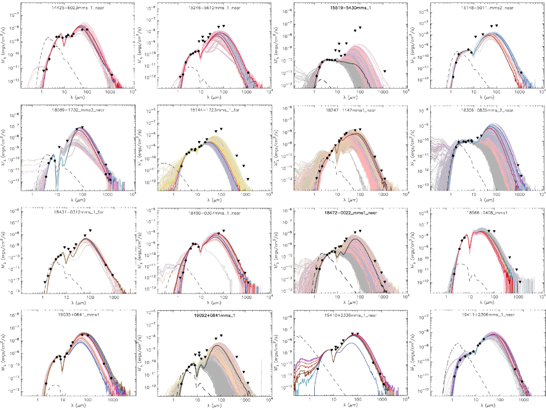
Figure 1: A sample of observed SED and their best fit models. Filled circular symbols represent the data points and the filled triangles represent photometry used as upper limits on the fitting. The dashed line corresponds to the stellar photosphere model used in the best YSO model fit.

Only a few exceptional sources(e.g. IRAS18454) fell in to third category where two or more red sources were found very close to the (sub)mm peak. In such cases, the reddest and brightest GLIMPSE point sources closest to the peaks were modelled by using the (sub)mm, MSX and IRAS fluxes as upper limits.

2.2 Data points and upper limits

The SED fitting tool developed by Robitaille et al. (2007) was used to fit the data with a grid of YSO models presented by Robitaille et al. (2006). This tool requires at least three wavelength points to fit the SED and any number of fluxes that can represent upper limits. The constraint on a data point is that the photometry extracted within a defined aperture must by all criteria represent a single source, with measured fluxes and associated errors. The good quality GLIMPSE or 2MASS data points, which have the highest spatial resolution among all the available data usually were used as the “data points”. However, we adopted a strategy to make the best use of all the data in constraining the SED. In many cases, we have used the (sub)mm data as a “data point” despite their large beam sizes compared to the GLIMPSE or 2MASS aperture sizes. If the (sub)mm emission indicated a single isolated clump with a well defined peak and, if within the spatial limits of the identified clump only one unambiguous high AM product GLIMPSE source was found, without any contamination from clustering of fainter objects, then we treated the (sub)mm data as a point source. In those cases where the (sub)mm emission was extended (despite having a single peak) and/or if there were more than one red source or fainter group of stars within the extent of the clump, we treated the (sub)mm data as upper limits. Further, we use the peak fluxes of the (sub)mm data and the beam size as an aperture in contrast to using the integrated flux from the entire clump. The MSX and IRAS fluxes were used as upper limits except for the very few cases where the source appeared totally unambiguous and isolated satisfying all the selection criteria. 10% errors on the fluxes were assumed GLIMPSE data and 50 % were used for 2MASS fluxes due extinction uncertainties. MSX and IRAS flux errors are typically around 10% depending on the bands and quality. The millimetre observations from the single dish telescopes usually quote conservative flux errors that were taken from the original literature. All the fluxes used as upper limits were set with confidence levels of 100%. These error assumptions provide sufficient margin to account for poor photometry and/or variability of sources.

3 SED fitting analysis

The online SED fitting tool was fed with the data selected according to the criteria discussed above with appropriate treatment as points or upper limits. For each run of fitting, the tool retrieved a best fit model (with the least $\chi^{2}$ value) and all the models for which the difference between their $\chi^{2}$ value per data point and the best $\chi^{2}$ per data point was smaller than 3. The number of such models for each target is called the fitting “degeneracy”. This is similar to the approach used by Robitaille et al. (2007) in fitting the low mass YSO SEDs. This approach is taken because the sampling of the model grid is too sparse to effectively determine the minima of the $\chi^{2}$ surface and consequently obtain the confidence intervals. A total of 68 sources was fitted: 50 from Sri02, 3 from Mol96, and 15 from Fon05. For all the targets (51) with distance ambiguity (where a near and far distance estimate was available), the SED fitting was done independently for the two distance values. The ambiguity was resolved for the remaining 17 sources. Since a distance range is used as an input in the fitting tool, we assumed a 20 % uncertainty for each of the assumed distances.

Fig. 1 shows the results from the SED fitting procedure. A sample is shown in the printed version and all the figures are presented online. Circles correspond to the photometric data points with respective error bars. In most of the cases, the error bars are so small that they are hidden behind the circles. The triangles are data points used as upper limits. The dashed curve in each figure show the stellar photosphere model used in the best fit models.

In Fig.2, we present the best fit model for the source 19411+2306mms1. The flux from the main components of the YSO is shown, namely the disk flux (dashed line), the envelope flux (dot-dashed line) and the scattered flux (three dot-dashed line). This example illustrates how different physical components dominate the emitted radiation at different wavelengths. The disk emission almost overplots the total flux in the near-IR domain whereas the envelope emission dominates the mid-IR to the millimetre range.

Although, the $\chi^{2}$ criterion is a good representation of the goodness of fit and associated errors, it is interesting to note that in a few cases, the model with the lowest $\chi^{2}$ may not actually represent the data very well. In some cases, the results were reiterated because the initial fits showed important information about the photometry classification. In Fig. 3 we show examples of two sources. The left panels displays the initial fit for which a low $\chi^{2}$ value and a high degeneracy was obtained. In these cases, due to our selection criteria described in Sec.2, the FIR and (sub)mm data were treated as upper limits. The model with the best $\chi^{2}$ (bold line) deviates significantly from the upper limits and appears not to be a good representation of the observed data. Although we use certain data as upper limits because of the uncertainties arising due to lack of information, we know that these may indeed be used as points if more information was available. In the right panel, we force the fit to go through the upper limits which results in a slightly higher $\chi^{2}$ value. Such a forced fit appears to better represent the observed fluxes at all wavelengths. For the purpose of overall analysis we use these fits rather than the best $\chi^{2}$ fit model.

Figure 2: Best fit model for the source 19411+2306mms_1. The full line represents the total flux of the source, the disk flux is represented by the dashed line, the envelope flux by the dot-dashed line and the scattered flux by the three dot-dashed line.

3.1 Estimating the physical parameters

The observed SED is typically fitted by multiple models, each model describing a set of physical parameters. The same parameters from different models can have a wide range spanning several factors to orders of magnitudes. To identify the representative values of different physical parameters for each source, the distributions of each parameter were analysed. As shown in Fig. 4, a single parameter histogram or a two parameter distribution plot were used to analyse the their distributions, specifically to see if the parameters coming from all the models fitting a given source had clear concentrations or significant spreads. The distributions of the stellar mass, the age and the luminosity generally show clear peaks that are independent of the model grid sampling characteristics. However, parameters such as disk mass or envelope accretion rate do not show such clear concentrations and usually have skewed distributions or spread out over a wide range of values. The right column in Fig. 4 shows the histogram of stellar mass estimated from all fitted models for sources 16219-4848mms1 (left panel) and 18290-0924mms1 (right panel). The distribution can be found to peak at 11 and 9 $\rm M_{\odot}\,$for the two sources respectively. These distributions are not an effect of the model grid parameter space coverage but a representative value that best describes the observed data. In the next section (Sec.3.2), we will demonstrate how we separate such biases. In fact the number of models in the grid decreases constantly with mass (see left plot in figure 5). The left panels in Fig. 4 display the correlation plots of age vs. stellar mass estimated from all the models that fitted the same two sources. A single concentration can be seen in this plot for the source 16219-4848mms1(top left) which represents an age of $10^{5.9}$ years and mass of 11 $\rm M_{\odot}\,$. In the case of 18290-0924mms1 (bottom left panel), the distribution has a relatively larger spread in the parameter space with a wide concentration between 6 and 10$\rm M_{\odot}\,$and ages between $10^{3.5}$ and $10^{5.5}$ years. In order to find a representative value for these distributions, we have decided to compute a weighted mean and standard deviation for all the parameters of each source, with the weights being the inverse of the $\chi^{2}$ of each model. All models where the ${\chi^{2}}_{best}-\chi^{2}$ per data point is smaller than 3 are used to compute the weighted means and standard deviations. It is important to note that these means are computed on a log scale for quantities that are spread over orders of magnitude in the model grid, such as age and accretion rates. This is done because these parameters in the grid were usually sampled with an approximately constant density in the log space.

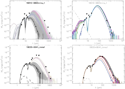
Figure 3: Examples of model fitting where the mid, far-IR and mm were used as upper limits (left) and data points (right).

3.2 What is model grid dependent and what is not?

The basis of the SED fitting analysis here, is a radiative transfer model grid, computed assuming certain physics which are thought to be quite valid for stars with a few solar masses (low mass stars). The model grid assumes that the same physics could be valid to understand the formation of stars up to 50$\rm M_{\odot}\,$Ṫhe reason why one expects that the assumed accretion scenario may work for such high masses is based on the observational evidence of outflows, disks and toroids around massive protostellar candidates. Such evidences are now abundant and has been obtained with spatial resolutions of an arcsecond or better, tracing size scales as small as a few hundred to 1000AU (Shepherd et al., 2000; Zhang et al., 2007).

The SED fitting tool used here, basically contains a database of 200,000 models, each with different physical properties and the observed SED is simply compared to the models in the grid to extract the closest matches. Due to the limitations inherent in the grid of models, various trends of parameter space are automatically generated and can be mistaken for a real trend (for more details see Robitaille et al., 2008). It is however, still possible to obtain useful information from the model grid by comparing the observed trends against the inherent trends in the grid. For this purpose and throughout this work, the parameter space from the full grid is compared to the derived values of the best fit models. By making such a comparison, it will be possible to visualise if the observed trend or a representative value is due to inherent biases in the model grid or the contrary. We will see in the next sections that the observed data indeed preferentially picks up certain narrow constraints on the physical properties of YSO components, even when the model grid provides an uniform or wide range of options.

Figure 4: Right panels: Histogram of stellar mass estimated from all fitted models (within the $\chi^{2}$ criteria) to the SED of sources 16219-4848mms1 (top) and 18290-0924mms1 (bottom). Left panels: Correlation of stellar mass vs. age estimated from all the fitted models for the source 16219-4848mms1 (top) and 18290-0924mms1(bottom).

4 Results

In Table.1 (sample shown in printed text), we list the parameters from the best fit models for the sources shown in Fig. 1. The online table contains all the columns originally given by the SED fitting tool. The values listed in each column are the weighted means of the respective parameters as described in Sec. 3.1. Additionally, each column is accompanied by a corresponding extra column quoting the standard deviation. The various columns in the sample table of the printed text are as follows: [col. 1] name of the source;[col. 2] $\chi^{2}$ per data point; [col. 3] mass of the star; [col. 4] age of the star; [col. 5] radius of the star; [col. 6] temperature of the star; [col. 7] envelope accretion rate; [col. 8] disk mass ; [col. 9] disk accretion rate.

Table 1: Parameters obtained for 16 sources within our sample. For each parameter we present the weighted average and the weighted standard deviation using all the models which fitted the data of each source within the $\chi^{2}$ criteria mentioned in the text. When no ’far’ or ’near’ reference is used in the name of the source, the distance ambiguity is resolved for that source. The values of $\chi^{2}$ tabulated are per data point.

Name	$\chi^{2}$	Age		$M_{*}$		$R_{*}$		$T_{*}$		$\dot{M}_{env}$		$M_{disk}$		$\dot{M}_{disk}$
		log(yr)		$\rm M_{\odot}\,$		log($\rm R_{\odot}\,$)		log($T_{\odot}$)		log($\rm M_{\odot}\,$$yr^{-1}$)		log($\rm M_{\odot}\,$)		log($\rm M_{\odot}\,$$yr^{-1}$)
14425-6023mms1near	5.28	3.7	0.6	14	3	1.9	0.4	3.7	0.2	-3.1	0.4	-0.9	0.7	-4.5	1.0
15246-5612mms1near	0.38	4.1	0.4	11	2	1.6	0.3	3.8	0.2	-2.9	0.7	-1.1	0.8	-5.2	1.2
15519-5430mms1	0.03	6.2	0.4	6	1	0.5	0.2	4.2	0.1	-6.7	1.1	-2.5	1.0	-7.9	1.3
16148-5011mms2near	2.24	4.2	0.3	11	1	1.7	0.2	3.8	0.1	-2.6	0.3	-1.4	0.8	-5.5	1.2
18089-1732mms3near	4.16	3.7	0.5	12	5	1.8	0.4	3.8	0.3	-3.5	0.7	-0.6	0.5	-4.1	0.6
18144-1723mms1far	1.41	5.2	0.4	18	2	0.8	0.1	4.5	0.1	-4.2	0.9	-1.1	0.6	-5.4	0.8
18247-1147mms1far	0.00	4.6	0.7	19	4	1.1	0.6	4.3	0.4	-3.6	0.4	-1.6	0.8	-6.0	1.1
18306-0835mms2near	0.48	6.0	0.6	7	1	0.6	0.3	4.3	0.2	-6.0	1.5	-2.5	1.0	-7.7	1.2
18431-0312mms1far	2.69	3.9	0.6	12	2	1.8	0.4	3.8	0.2	-2.8	0.1	-0.6	0.3	-4.4	0.7
18460-0307mms1near	3.78	5.0	0.4	13	3	0.8	0.2	4.4	0.1	-3.4	0.3	-1.0	0.6	-5.5	0.8
18472-0022mms1near	0.08	5.6	0.9	8	2	0.8	0.4	4.2	0.2	-5.0	1.3	-2.0	0.9	-7.0	1.2
18566+0408mms1	1.12	3.7	0.4	40	6	1.8	0.6	4.2	0.3	-3.8	0.1	-0.9	0.7	-5.3	0.6
19035+0641mms1	6.65	4.7	0.1	11	0	1.2	0.1	4.1	0.1	-2.6	0.0	-2.0	0.3	-6.0	1.0
19092+0841mms1	0.08	6.0	0.8	9	2	0.7	0.3	4.3	0.2	-5.1	1.4	-2.1	1.0	-6.8	1.3
19410+2336mms1near	43.87	4.8	0.0	11	0	1.1	0.0	4.2	0.0	-2.5	0.0	-1.7	0.0	-5.4	0.0
19411+2306mms1near	1.74	3.9	0.4	10	1	1.8	0.2	3.7	0.1	-3.3	0.3	-0.8	0.6	-5.1	0.9

As we mentioned before, the SED fitting was carried out using both the near and far distance estimates. The overall statistical analysis of the YSO physical parameters was made by using the fit with a distance that provided the best $\chi^{2}$ per data point for each source. The exception is Fig. 5 and the first two panels of Fig. 7 where we separate the distributions of the respective parameters in near and far distance results. (In the online table we also present the the results for both distances for the sources to which it applies.)Therefore the general trends that we explain in the rest of this paper will have a mixture of near, far and distance resolved fittings.

The model provides estimates of the interstellar extinction, the extinction interior to the envelope and the luminosity of the source. The interstellar extinction Av is estimated to span over a range between 0-150, and the histogram shows a peak between 10 and 25 mags. The distribution of the extinction values internal to the modelled YSO is found to peak between 30 and 300 mag. This is roughly similar to the extinction estimated from the millimetre continuum observations of such cores.

In the following we will elaborate on the overall results pertinent to the main components of the protostellar SED.

Figure 5: Histograms of stellar mass (left), age (centre) and temperature (right) for all the 68 sources in our sample. The dashed histograms in the 3 plots represent the same distributions for all the models in the grid of Robitaille et al. (2006).

4.1 Properties of Photospheres (driving engines)

The photospheres are the driving engines of massive protostars which is also the end product of the massive star formation process that we seek to understand. The embedded photospheres of the massive protostellar candidates are already expected to be massive even though it is accreting material. Using the weighted mean values of the parameters for the photosphere from the SED fitting procedure, we can investigate the general properties of such massive stars.

Fig. 5 shows the overall statistics based on the estimated representative values for the stellar mass, age and temperature for all the fitted sources. These histograms are shown with a normalised frequency in order to compare them with the grid distribution. The dashed line represents the results from the near distance fittings, dotted lines for the far distance fittings and the solid line represents the histograms of the full model grid. Comparing the trend of the fit results to the trend inherent in the grid, it can be seen that the fit results represent values of mass, age and temperature that are not biased by the trend in the model grid but are probably those that selectively describe the observed data.

These results describe most of the sources as massive protostars with a mean stellar mass of $\sim$10–20 $\rm M_{\odot}\,$and includes stellar masses as high as 40 $\rm M_{\odot}\,$, with total luminosities between $10^{3}$ and $10^{5}L_{\odot}$. Many of them are very young, with ages of $\sim 10^{3}-10^{4}$ years, and only a small fraction are modelled as 1Myr objects. It should be noted that the model grid becomes very low in density after 5-10$\rm M_{\odot}\,$  and even so, the observed SEDs have the highest densities for the 10-30$\rm M_{\odot}\,$  range. The near distance fitting naturally selects a relatively lower mass for the source compared to the far distance fitting. If HMPOs are in the accretion phase, the estimated young ages are not a surprise because the accretion phase is supposed to be very fast, typically 5$\times 10^{4}$yr or less (McKee & Tan, 2003)

The model grid is roughly populated with constant density in log(age) space (see fig.2 of Robitaille et al. (2006)). Curiously, the observed data strongly picks up models that have lower ages with a peak between $\sim 10^{3.5}-10^{4.5}$ years. Luminosity peaks (not shown here) are consistent with the observed IRAS luminosities of these sources.

The radii of the photospheres selected by the observed data are typically large between 20-200$\rm R_{\odot}\,$. The stellar temperature is found to be typically between 4000K to 8000K but there is a considerable number of models spanning a range between 10000K-26000K. It is important to note that while the mass and age are uniformly sampled for the grid limits, the radius and temperature are interpolated using evolutionary models. Nevertheless the model grid covers a range of stellar radii from a few solar radii to few hundreds of solar radii and temperatures from 2500K to 40000K. It is interesting to note that the observed SEDs preferentially select models with large stellar radii(20–200Rsun) and relatively lower temperatures (4000K-8000K).

The SED is sensitive to the T_⋆ and L_tot, which are therefore basic results. The R_⋆ and age are derived from these parameters using evolutionary models.

4.2 Disks and envelopes around massive protostars

Fig. 6 compares the mass of the disk and the age of the star with the associated spread in the values. The symbols represent the weighted mean values and the error bars represent the weighted standard deviations. The contours show the distribution inherent to the model grid, with the outer most contour representing mean values of the entire grid and subsequent contours are spaced at intervals of 1$\sigma$ from the mean value. The data points from the fitting results occupy a region representing higher disk masses compared to the mean value of the grid. Thus, the modelled sources are best represented with massive disks. It can be seen that for the youngest sources, there is a spread of disk masses around $\sim$ 0.1 $\rm M_{\odot}\,$with no visible trend. However, for the few older sources at $\sim 10^{6}$ yrs, the disks become less massive and have larger uncertainties, as one would expect.

Fig. 7 shows a plot of the accretion rate versus age of the protostar for all the 68 fitted sources. The left, middle and right panels represents results from near distance, far distance fitting and the “best $\chi^{2}$ distance” respectively. Protostars without disks are represented by squares, meaning they represent envelope accretion rates alone. For protostars with an envelope and a disk together, empty circles correspond to the disc accretion rate and the triangles correspond to the envelope accretion rate. Filled circles represent disk accretion rates for sources without envelopes. Naturally, there will be an empty circle associated with each triangle. The sizes of all these symbols are shown roughly proportional to the associated stellar mass which is distributed in to four groups that are representative of O, B0-1, late B stars and A type or lower mass stars. The Disk accretion rate is lower than envelope accretion rate as expected from the assumed physics in the models. Protostars without envelopes (filled circles) have ages greater than one million years. The solid contours represent the range of envelope accretion rates inherent to the model grid.

Most of the modelled sources show the presence of both disks and envelopes when fitted with both near and far distance estimates. The mean disk masses and accretion rates are $10^{-1.4\pm 0.7}$ $\rm M_{\odot}\,$  and $\sim 10^{-6}$ $\rm M_{\odot}\,$yr^-1, respectively. The disk inner and outer radius range from a few AU to 50AU respectively. The dust sublimation radius is mostly within 10AU but can go as high 45AU depending on the mass and age of the modelled source. The envelope accretion rates and sizes are $\sim 10^{-3}$ $\rm M_{\odot}\,$yr^-1 and 65000 AU respectively. In particular, the envelope sizes are large with a spread between 50000 and 150000 AU, which corresponds to the limit at which the model truncates the envelope radius. This distribution peaks at $\sim$50000-60000 AU. At an average distance of 5kpc, it is very similar to the projected sizes of the infrared nebulae found in Paper I. The luminous star heats up large volumes that may not necessarily be part of the infalling envelope, but rather the ambient molecular cloud. The SED is sensitive to the stellar temperature and total luminosity, from which the remaining parameters are derived. Therefore the large envelope radii just represents the radius at which dust is heated by the star.

Figure 6: Correlation between the disk mass and the source age estimated for all the sources with disks. Standard deviations for the two parameters are given by the error bars. If a given source was fitted by a single model, no error bars are shown. The contours represent the distribution of the same parameters in the entire grid of models used in this work. The outer contour corresponds to mean value and they increase in standard deviation units.

The dependence of the disk and envelope accretion rates as a function of stellar mass is seen as a power law. This power law dependence is estimated from the SED fitting results and compared against that which is inherent to the model grid in the same mass range. The envelope accretion rate from the SED fitting results scales as $\dot{M}_{env}$ = 10${}^{-5.5\pm 0.6}\times{M_{*}}^{2\pm 0.6}$. In contrast, the power law inherent to the model grid is $\dot{M}_{env}$ = 10${}^{-5.3\pm 0.02}\times{M_{*}}^{1\pm 0.02}$ over the same mass range. This accretion rate dependence is indicative of spherical accretion (Bondi, 1952). Since the envelope sizes are linked to the luminosity, this relation simply means that the accretion is approximated to a spherical case at the scale of the dense core. Similarly, the disk accretion from fitting results is related to the source mass as $\dot{M}_{disk}$ = 10${}^{-7.2\pm 0.7}\times{M_{*}}^{1.5\pm 0.7}$ and that inherent to model grid is $\dot{M}_{disk}$ = 10${}^{-9.7\pm 0.03}\times{M_{*}}^{2.5\pm 0.03}$. Recently, Fazal et al. (2008) have modelled 13 similar targets from the Sri02 lists using the same fitting tool and found very similar relation for the envelope accretion rates. However, parameters estimated for individual sources by Fazal et al. (2008) can be different from the values listed in Table.1, owing to different data sets and selection criteria. In particular, they use MIPS observations (not used here) and also the integrated flux in the millimetre regime whereas we use the peak fluxes from millimetre data. Also, the relations given here are obtained from a larger sample, constraining the uncertainties in the power-law coefficients.

Figure 7: Correlations between the accretion rate and the age of the protostar. In the left panel we present the results with the near distances assumed for sources with distance ambiguity. In the middle panel, the same is shown with with far distances assumed. In the right panel, the parameters shown for these sources are for the distance with the lowest $\chi^{2}$ fit. The empty circles represent the disc accretion rate for all the sources with discs. The triangles represent the envelope accretion rate for all the sources with an envelope and a disc. Squares represent the envelope accretion rate for the sources without discs. Filled black circles represent sources without envelopes. The envelope accretion rate distribution inherent to the grid is shown by the contours as in fig. 6

4.3 Individual sources

The following notes serve to identify the modelled sources in conjunction with online figures from Paper I, or from the original GLIMPSE images:

13384–6152mms1 A high AM source matching well with the millimetre peak. A clear point source with a unipolar nebula.

13395–6153mms1 A highly saturated GLIMPSE point source matching with the 1.2mm peak. Good photometry available in the JHK bands. GLIMPSE photometry not available due to saturation.

13481–6124mms1 Highly saturated point source in GLIMPSE image. JHK photometry available and no GLIMPSE photometry. All data were used as points. The model fit indicates a 20 $\rm M_{\odot}\,$and young star at $\sim$10⁴ yrs.

13560–6133mms1 An isolated high AM source coinciding with the mm peak. The point source is surrounded by a shell like IR nebula. No clustering or other YSO like sources within the shell.

14000–6104mms3 A high AM point source in the middle of a large diffuse nebula. GLIMPSE data for the point source is good. The mm data was used as coming from a single source.

14131–6126mms1 GLIMPSE point source surrounded by an extended (scorpion shaped) 8 $\mu$m nebula. The 1.2mm data was used as a ”single source” point. The point source had JHK data. IRAC ch1 and ch4 data not available probably because of contamination from the nebula.

14166–6118mms1 Point source with photometry from GLIMPSE to mm. It is surrounded by an IR nebula with a core-halo structure.

14425–6023mms1 An isolated (nearly saturated) bright GLIMPSE point source with H and K photometry as well. Given that there are no other FIR/mm contributing nebula or stars in the field we used MSX, IRAS and mm data as points.

15246–5612mms1 A high AM point source surrounded by an IR nebula which looks like a dense core irradiated by the central star. Data in the H, K, GLIMPSE and the 1.2 mm bands were used as single source points.

15347–5518mms1 A bright GLIMPSE point source surrounded by an IR nebula with a core-halo shape. The 1.2mm data was assumed as a single source point.

15506–5325mms1 Almost saturated GLIMPSE point source with a good JHK counterpart. The mm emission and FIR fluxes do not represent the fitted model that traces the JHK and MSX points. The IR point source appears to be an evolved YSO. The IRAS and mm emission may be arising from an adjacent, more deeply embedded object.

15519–5430mms1 Well defined isolated GLIMPSE point source in the middle of a large infrared nebula. The SED was well fitted by an evolved 6 $\rm M_{\odot}\,$object. The IRAS and mm emission is not well represented by the model.

15579–5347mms1 A bright isolated point source surrounded by a dense cocoon and compact nebula which extends out to an arm like structure on the 8 $\mu$m image. The source appears in K band as well.

16061–5048mms3 A chain of 6 point sources bordering an arc shaped IR nebula on one side and an IR dark patch on the other side. The sources seem to be inside the dark cloud that extends to a much larger size. The mm peak coincides with a fuzzy point source for which photometry is available only in the ch3 and ch4. The IRAS and MSX point are 30^′′off, therefore the mm data is used as a data point and the IRAS as upper limits.

16082–5031mms1 One bright star situated on the periphery of a ring shaped nebula. The source also appears to be aligned with a dark filamentary cloud on a larger scale. Although the source is seen in GLIMPSE, the catalogs do not list the photometry. But a good 2MASS counterpart exists. We used 2MASS and 1.2 mm data as points with IRAS as upper limits.

16093–5015mms2 Two bright high AM product sources adjacent to each other. The mms2 source coincides well with one of the stars which is also well centred on an IR dark cloud. A bright U shaped nebula is adjacent to the source. The IRAS and MSX sources coincide with the centre of this nebula.

16148–5011mms2 A bright IR nebula inside which are embedded two point sources. The brighter of the two coincides with mms2 and has photometry in JHK, IRAC ch3 and ch4 bands. IRAC ch1 and ch2 photometry are probably contaminated by the nebula. We used 1.2mm data as a point.

16218–4931mms1 A clear point source with both 2MASS and GLIMPSE data. The source did not appear as high AM source in paper I. The point source is linked to an IR nebula with a tail like morphology. The fit was not very good.

16219–4848mms1 An isolated IR source with 2MASS K, IRAC ch2 and ch3 band photometry available, surrounded by an arc-shaped nebula. The fit has a large degeneracy and the IRAS 100 $\mu$m emission is not represented well by the fit.

16232–4917mms1 A bright point source surrounded by a dense cocoon and an arc shaped nebula with streamers connecting the arc and the star. The star has photometry in 2MASS JHK and GLIMPSE and a shows a well defined mm peak. MSX data was removed as it was not positionaly consistent with the other data and that was confirmed by the fitting results.

16344–4605mms1 A filamentary IR dark cloud. At least eight deeply embedded red sources are found to be coinciding clearly along the filament. These sources are close to the mm peak. Based on positional correlation with MSX and IRAS, the mms1 was chosen for modelling. It has data from the GLIMPSE to 1.2mm bands. Although the degeneracy of the fit was high, we did not use mm data to force a fit because of multiple red GLIMPSE sources in the same field.

16363–4645mms3/mms6 The region is filled with multiple red sources. Two mm peaks namely mms3 and mms6 are associated with compact GLIMPSE nebulae and point sources. They are also associated with two separate MSX sources. The mms6 source was modelled using the GLIMPSE and mm data as points. The MSX was not used because the 8 $\mu$m image shows a bright compact IR nebula nearby this source and could be contaminating the MSX flux.

16464-4359mms1 Faint GLIMPSE point source with a small nebula.

16501–4314mms1 Two IR point sources in the field, one at the tip of a fan shaped nebula. This source coincides with mms1 and the MSX peak and was modelled.

16573–4214mms5 An isolated point source surrounded by a bright IR nebula. No other confusing sources in the vicinity, and a decent fit was obtained by using the 1.2 mm data as a point.

18089-1732mms3 Three high AM sources surrounded by three fan shaped infrared nebulae. One of this high AM sources coincides with the mms3 clump from the 1.2mm MAMBO maps which is modelled. This source is also studied using interferometer data (see Sec.5.4)

18090–1832mms1 Data for this source is available from the near-IR to the mm wavelengths, however due to possible confusion with nearby objects, only the IRAC and 2MASS K bands were used as data points.

18144–1723mms1 A low source by the definition of Mol96. A single bright IR source (slightly nebulous object) is found coinciding with the mm peak. The sub-mm observations are obtained with SCUBA. The model is constrained using GLIMPSE and MSX data.

18151–1208mms1 No GLIMPSE point source data available for this source. The source appears point like in the 2MASS K band and (sub)mm. An extended nebulae/halo is found surrounding the point source in the K band as well as GLIMPSE images. The source shows an outflow studied by Davis et al. (2004).

18159–1550mms1 Three point sources centrally surrounded by a bipolar shaped nebula. Sub-mm source looks point-like. Millimetre image looks fuzzy with no clear point source. (Not an high AM source).

18247–1147mms1 A well isolated point source identified from the NIR to (sub)mm peak. The coordinates match to an accuracy of better than 1^′′. We used the integrated fluxes in the (sub)mm because of its point like appearance and treated everything as a point because nothing else was found in a 20^′′radius.

18264–1152mms1 Bright high AM product source in the middle of a bright 8 $\mu$m nebula. The GLIMPSE source matches well with (sub)mm peaks which appears point like despite the large infrared nebulae.

18290–0924mms1 Apparently confusing object. A high AM source situated 8^′′from the sub-mm peak. But the sub-mm peak has no counterparts and shows up as a high contrast dark patch located adjacent to the bright star and faint nebula. We modelled the high AM source only using GLIMPSE, MSX+IRAS. Therefore, we assume the modelled point source and the sub-mm emission as different entities.

18306–0835mms2 The main (sub)mm peak coincides with a compact nebula and does not have an IR point source. Roughly 1.5’ away the (sub)mm source 2 has a MSX point source and has a good IRC which is modelled.

18308–0841mms3 The main (sub)mm peak coincides with a bipolar IR nebula that is at the tip of a dark filament. A fainter (sub)mm peak (peak 3 of MAMBO) is associated with an IRC which is modelled using GLIMPSE, MSX, MAMBO+SCUBA. There is no detected flux at 450 $\mu$m for this source.

18310–0825mms1 The (sub)mm peak is closely located to a GLIMPSE source that is modelled. The MSX+IRAS peaks appear 15^′′offset from the (sub)mm peak and GLIMPSE source and is coincident with an IR nebula.

18337–0743mms1 The (sub)mm peak coincides with a bright and compact IR nebula in shape and position. The IR nebula is well centred on a star which is visible in the JHK bands. The GLIMPSE counterpart is not available (although visible on the images) in the catalog. The nebula is a core-halo shaped object. The MSX+IRAS point sources are offset by 15^′′falling on the edge of the nebula. The model was constrained by using the 2MASS+sub-mm peaks as data points while MSX, IRAS and MAMBO were used as upper limits. No other suspicious objects in a vicinity of $>30$^′′.

18345–0641mms1 The (sub)mm peak coincides well with two very bright GLIMPSE sources that are close to saturation. A 2$\mu$m source is coinciding. The (sub)mm, IRAS, MSX, GLIMPSE, 2MASS positions match to better than 2^′′. Not found as a high AM source in paper I, because the GLIMPSE source is not available in the highly reliable catalog.

18372–0541mms1 A bright (sub)mm condensation with an extended elliptical shaped halo. The high AM source is bright and situated within 4^′′of the (sub)mm peak. Two red fainter GLIMPSE sources are found in a radius of 6^′′ from the high AM source. No 2MASS counterpart. The IR nebula at 8 $\mu$m resembles a core-halo shape with a halo of $\sim$10^′′. The (sub)mm peak flux is used as a point because of the morphological resemblance over the whole range of wavelength and no other significant objects are found within a 20^′′radius.

18431–0312mms1 Elliptical shaped (sub)mm peaks at 850$\mu$m, 450$\mu$m and 1.2 mm. Core-halo IR nebula with a K band and GLIMPSE star. 8 $\mu$m photometry not available (possibly because of the nebular contamination). MSX source matches closely. No other suspicious source within a radius of 10^′′. Therefore, the (sub)mm peak fluxes were used as points for the fitting.

18440–0148mms1 The sub-mm peak is point-like. The mm (MAMBO) peak is extended and elliptically shaped. The IRC is a bright star with photometry available only in ch3 and ch4 bands. No other confusing sources nearby within a 10^′′radius.

18445–0222mms1 Two high AM sources with a bright IR nebula. (sub)mm peaks are clearly point like. One of the high AM source matches to better than 2^′′with the sub-mm peak which is modelled. MSX not used. IRAS used as upper limits. GLIMPSE + sub-mm used as points.

18447–0229mms1 One high AM IRC matches well with the (sub)mm peak. IRAS was used as upper limits while GLIMPSE and (sub)mm were used as data point.

18454–0136mms1/mms2/mms3 Three clean GLIMPSE point sources with high AM product are within the FIR/sub-mm beams. We use the GLIMPSE data as points and the FIR/mm data as upper limits for each of the IR sources. This is a cluster of at least 5 GLIMPSE sources within the sub-mm beam and two of them are high AM sources. Three bright sources are modelled. mms1 coincides with the mm peak. mms2 is the brightest GLIMPSE source and has radio continuum emission.

18460–0307mms1 A bright high AM source coincides with IRAS, MSX and sub-mm peaks. We used only the IRAS 60 and 100 $\mu$m, K band, (sub)mm and GLIMPSE points to get the fit. Some of the MSX and IRAS photometry was removed to improve the fit.

18472–0022mms1 One bright high AM source coincides with the sub-mm peaks. The (sub)mm emission is extended but with a single well defined peak. The IR source is surrounded by a cocoon in the IR and a fan shaped nebula adjacent to it. The high AM source is modelled.

18488+0000mms1 A bright star (saturated in GLIMPSE). This source was not classified as high AM product in paper I because of saturation. Photometry for ch1 and ch3 is available from GLIMPSE less reliable catalog and a bright K band source coincides with the star. The bright star is surrounded by an unipolar fan shaped nebula. The (sub)mm emission is a circularly concentrated peak with a very faint extension towards the unipolar flow. The ch3 photometry was treated as upper limit (likely saturated) and 1.3 mm is treated as a point to improve the $\chi^{2}$ of the fit.

18511+0146mms1 A bright saturated GLIMPSE source coinciding well with the mms1 millimetre core. The source did not appear as a high AM product source in Paper I and no GLIMPSE photometry is available due to its saturated nature. However, the star has good 2MASS J,H,K photometry. MSX data was used as points along with IRAS and millimetre data as upper limits to obtain the fit.

18521+0134mms1 One high AM source coinciding with the (sub)mm peaks to better than 2^′′. The (sub)mm peaks are well concentrated with a surrounding halo. The high AM source is modelled with all data points.

18530+0215mms1 There is no point source in the GLIMPSE or 2MASS. GLIMPSE data shows a spectacular bipolar nebula typical of an outflow. The (sub)mm emission is concentrated (point-like) with a faint extension in the direction of BP outflows. We used the MSX, IRAS and (sub)mm data, treated the (sub)mm data as points.

18553+0414mms1 Two bright high AM sources close to each other. The brightest of the two coincides with the (sub)mm peak. The GLIMPSE ch4 data is saturated. There are no 2MASS counterparts. No suspicious clustering objects nearby. The brighter source coinciding with the (sub)mm peak is modelled.

18566+0408mms1 This source is a very bright GLIMPSE source (saturated in the ch3 and ch4) and only a K band counterpart is available. The positional correlation with the (sub)mm peak is very good ($<$2^′′). However, the source appears as a double source, both comparable in brightness. This may be indicative of the (sub)mm peak appearing elongated elliptically. This is probably a case of massive binary. The source is modelled as a single source.

19012+0536mms1 The (sub)mm and FIR peaks appear point like. GLIMPSE data reveals at least 5 point sources and a bright concentrated IR nebula within the beams of (sub)mm and IRAS data. The IR source coinciding with the (sub)mm peak is modelled . Indeed this source appeared as a medium AM source in paper I and the high AM source in the same field from paper I is 20^′′away from the (sub)mm peak which is not modelled.

19035+0641mms1 The sub-mm peak and all other data match to better than 1^′′. The IR source appears bright in the GLIMPSE.

19045+0813mms1 The IR source is visible in all Spitzer bands in the 2MASS K band. The 1.2 mm data (peak flux) was obtained by Sánchez-Monge et al. (2008). Very good fit. The object in the IR is a bright source with a surrounding infrared nebula that appears to show four arm like structures. It can also represent wind blown cavity walls.

19074+0752mms1 A high AM source aligned well with the (sub)mm peak. An arc shaped unipolar nebula originating from the IR point source. No photometry available for IRAC ch1 and ch2 bands. By using the Spitzer sources as points we produced a big discrepancy between the best fit model and the remaining data used as upper limits. We decided then to use the 450 $\mu$m data was used as a point.

19092+0841mms1 A well defined GLIMPSE point source which appeared as an average AM source in Paper I coincides well with the millimetre peak. The point source is surrounded by a fan shaped unipolar infrared nebula and also visible in the 2MASS K band. The K band and GLIMPSE photometry were treated as data points with all the other as upper limits to obtain a fit. This source was modelled with a high degeneracy.

19175+1357mms1 The (sub)mm peak coincides with a compact, bright 8 $\mu$m nebula in which there appears to be embedded 3 point-like sources. However, the catalog lists only one point source for which data is available only in ch3. The photometry in other bands is contaminated or was difficult to obtain because of the bright nebula. Since at least 3 points are needed to the RT fit and the (sub)mm emission is concentrated like a point source or a peak, we use 450 and 850 $\mu$m data as points.

19217+1651mms1 One of the best studied and clean sources using photometry all the way from 2MASS K band to the interferometric observations. No contamination from any adjacent sources.

19266+1745mms1 A GLIMPSE point source with an IR nebula. The (sub)mm data shows emission that looks like a tadpole with a peak and a tail (extending to the south).

19282+1814mms1 The (sub)mm source appears extended with one prominent peak where the MSX and GLIMPSE sources coincide. The IRAS source is about 60^′′off to the east (we did not use it). The region is filled with several GLIMPSE point sources, with at least 10 red sources surrounding the modelled bright source. In paper I, this bright source did not appear as a high AM source. Submm data was used as a data point.

19410+2336mms1 A satured GLIMPSE source represent the (sub)mm and FIR peaks to better than 1^′′. Data for this was found in the less reliable catalog. However a good K band data point constrains the fit. So we used 450/850 $\mu$m and K band as points and removed the GLIMPSE data. A well defined outflow originates from this mm source.

19410+2336mms2 A faint GLIMPSE source without MSX and IRAS counterparts matches the sub-mm peak. A well defined outflow is found to originate from this mm source.

19411+2306mms1 The IR source appears in the 2MASS JHK and the GLIMPSE data as a point source but shows extended (sub)mm emission. No other high AM product source in the vicinity. The (sub)mm, MSX, 2MASS and GLIMPSE were all used as data points. This model is highly constrained and defined by the short wavelength data.

19413+2332mms1 The GLIMPSE images display two fan shaped nebulae separated by a dark lane. A faint GLIMPSE source which has photometry in ch1 and ch2 and also in the 2MASS K band, is located coinciding with the tip of the fan shaped nebula and also with the millimetre core. The sub-mm data appears point like and the SCUBA data was used as a point.

5 Discussion

5.1 Caveats inherent to the modelled data

In the previous section, the physical parameters of the star, disk and envelopes were estimated by fitting the SEDs of the IR point sources. The resulting variables were compared to identify specific trends. In the following we will discuss some caveats pertinent to the observational data, fitting procedure and selected sample.

• Masses of the driving engines

  The SED fitting results show that some objects with the highest stellar masses (luminosities) are also among the youngest sources in the sample. Older sources with similar masses are expected to be already in an evolved HII region stage and are probably not detected because their FIR colours would not be in agreement with the initial criteria of the selection of HMPO candidates and/or they would have significant ionised emission (See e.g. Keto & Klassen, 2008). On the other hand, the less massive sources in this sample are concentrated towards older ages. At a distance of a few kpc, the GLIMPSE data would be sensitive to detect pre-main sequence objects rather than embedded protostars of lower masses. Besides this, the most massive protostars (early O stars) may be residing in the infrared-dark clouds (IRDC’s) (Jackson et al., 2008) that shine only in the FIR and millimetre wavelengths or associated with the driving engines of HII regions.

  The models of Robitaille et al. (2006) do not account for the accretion luminosity arising in the envelopes which is thought to be significant for sources with masses greater than 20$\rm M_{\odot}\,$. However, they do compute the disk accretion luminosities for all mass ranges. The results from this work and in Paper I, indicates that envelope accretion or accretion through gaseous disks may play an important role in building the most massive stars. Therefore the few sources modelled with M$\geq$20$\rm M_{\odot}\,$may need alternative investigation. Naively, this means that stellar masses $>$20$\rm M_{\odot}\,$are probably over-estimates and the sample studied here represents a good census of proto-B stars rather than proto-O stars. However, some of these proto-B stars at present time could become O stars in future.

• Multiplicity issue

  One of the important aspects of massive star formation is that they are known to form in multiple systems or strongly clustered environments. In Paper I we discussed the issues related to clustering around the IRCs of HMPOs analysed here and concluded that we did not find clustering at the level of $\sim$4-5$\rm M_{\odot}\,$ members. The “isolated” nature is therefore valid only for the mass range beyond 10$\rm M_{\odot}\,$ . These objects can, however, have multiplicity at a level of $\sim$6000AU (at a distance of 3 kpc) owing to the assumed 2^′′spatial resolution of the GLIMPSE data. Assuming a source in the simplest case of multiplicity - a binary system, there are two possible scenarios; a) two objects at the same evolutionary state and b) objects in different evolutionary states. In the first case, the SED modelling can not detect possible multiplicity because the SED shapes will be similar for the two sources and may overlap. In the latter case, where sources are at different evolutionary stages, the SEDs are expected to flatten out because of the older source and is prone to be detected by its unfamiliar shape. It turns out that we did not find any source from our fitting which deviates from the normal single source SED with a single exception (18447-0229mms1), and therefore multiplicity of sources with different evolutionary stages is not a likely possibility. See the online Fig.1 to check this.

5.2 Ionised accretion flows?

As mentioned previously in Paper I, free-free continuum emission in the centimetre regime coinciding with 27 HMPOs in that list was detected with VLA and other observations. Free-free continuum emission indicates the presence of compact ionised regions surrounding the massive protostars and/or winds in the bipolar cavities. Eleven of the 27 sources were modelled in this work and are shown as filled grey symbols in Fig. 8. The fitted models describe massive stars with an actively accreting disk and envelope. But their properties such as accretion rates, ages, or masses are not different from the mean values for the rest of the sample.

Therefore these sources could be typical YSOs with ongoing accretion and significant ionised gas close to the star, making them good examples for accretion past the HII region. If the accretion scenario suggested by the models is in fact correct, the presence of ionised emission could imply the existence of ionised accretion flows and/or ionised winds, in addition to the molecular components. The scenario of continuing accretion (accretion past the HII region) therefore could play an important role in the most massive star formation.

Although several massive protostars are found from this work, some of the most massive objects from the initial sample of HMPO candidates are still missing from this study. This is because such sources appear very bright in the near/mid IR bands and are saturated in the IRAC images (see Paper I). Such sources can make a good target sample to investigate the mechanism of accretion past the HII region, by using short exposure ground based IR and centimetre continuum observations.

5.3 HR Diagram

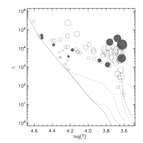
Figure 8: Luminosity vs. stellar temperature plot. Filled circles represent sources with known radio continuum emission as found in the literature. Solid line marks the birth-line track from Bernasconi & Maeder (1996) for masses above 7$\rm M_{\odot}\,$and represent the ZAMS up to 7$\rm M_{\odot}\,$. The dotted lines are Geneva isochrones up to 7$\rm M_{\odot}\,$. From left to right the dotted lines represent values of log(age)= 6,5,4 and 3.

In Fig. 8 the luminosity and stellar temperature of all the modelled sources are compared to simulate an HR diagram. It is important to note in advance, that this HR diagram is prone to mimic the assumed stellar evolutionary models. Nevertheless, some facts are worth noting. The shaded circles represent the sources associated with significant free-free continuum emission, but the contrary is not true. There is simply no radio observations available for all the sources to ascertain the fact. The size of the symbols are made inversely proportional to the age of the protostar in this figure. Clearly, the oldest sources (smallest circles) trace the zero-age main sequence locus. These sources have smaller accretion rates and the stellar photosphere is a significant contributor to the total luminosity. The youngest sources (big circles) are all found above the ’main sequence’ locus. At younger ages, other physical processes such as envelope accretion are the dominant contributors to the total luminosity and the photosphere is mostly obscured. Sources found occupying the right side of the diagram are likely protostars representing the onset of deuterium burning along with the presence of a convective envelope. The observed shapes and luminosities of the SED clearly exclude the possibility of classical intermediate PMS stars (dotted lines are PMS tracks up to 7$\rm M_{\odot}\,$). The sources associated with radio continuum emission are distributed in different parts of the HR diagram and do not show any particular trend with other estimated properties. Four sources, found on the extreme right hand side of the diagram are worth noting for their youth, mass and association with radio continuum emission. They may represent sources where powerful ionised winds or accretion flows are onset at a very early stage of formation. But it should also be noted that the age estimates from the SED fitting are probably uncertain. The difference between accreting and non-accreting massive star on the main sequence could be identified better by observing the structure of the ionised region at smaller scales (McKee & Tan, 2003; Keto & Klassen, 2008).

5.4 How real are the driving engines, disks and envelopes?

Throughout this paper, we focussed on how the observed data preferentially chooses certain set of values or relations from a larger set of available options in the model grid. While these results may appear real, it is important to view them within the limitations of the models, discussed in Robitaille et al. (2006) and remembering “what you put in is what you get out” quoting Robitaille et al. (2008).

The SED modelling selectively picked up large radii for driving engines and lower temperatures. Both these parameters are derived from the assumed evolutionary tracks after uniformly sampling the mass and age grid in the models. The accretion rates assumed in computing those evolutionary tracks are typically $10^{-4}$–$10^{-5}$ $\rm M_{\odot}\,$yr^-1. The SED fitting results also suggest that the accretion rates are much higher than those values and could be as high as 10^-2–10^-3$\rm M_{\odot}\,$yr^-1. In a situation like that, the mass- radius relationships for the massive protostars are also expected to be different. Hosokawa & Omukai (2008) discuss such effects in detail. In any case, although the SED modelling suggest photospheres with certain properties, it is far from clear if those are real photospheres where hydrogen burning has begun or if those surfaces are totally different type of entities (McKee & Tan, 2003; Zinnecker & Yorke, 2007).

The SEDs for high mass protostars are dominated by the envelope flux longward of 8-10$\mu$m and the disk flux is almost always embedded within the envelope flux. It is possible, therefore, that models with envelopes alone and models with disks and envelopes successfully fit the same SED. It is particularly true in the case of sources without photometry in the near-IR or IRAC ch1. Although, the results here favour the presence of massive disks with relatively larger radii, the overall SED may not be sensitive to the presence or absence of the disk. But the envelope geometry is indirectly dependent on the disk radius, since the models use a rotating-infalling solution. Therefore, in the few cases, when the SED models indicates no disk, it may simply mean that the disk is gaseous and its size is well within the dust destruction radius which could be between a few AU to 50AU for the sample studied here. Bik & Thi (2004) argued for the presence of disks in massive young stars (much older than the ones in this sample) by modelling the CO band heads with Keplerian disks. They estimated small inner and outer disk radii (0.2–3.6AU) and masses ($<$30$\rm M_{\odot}\,$) for those presumed molecular disks. Grave & Kumar (2007) conducted a spectro-astrometric analysis of the Bik & Thi (2004) data and found that the disk sizes should be much larger (200-300AU) than originally predicted by those authors. In the light of SED fitting results, the Bik & Thi (2004) results conform with the pure gaseous disks and those of Grave & Kumar (2007) may represent the gas+dust disks indicative of the rotating-infalling solution centrifugal radii.

We noted in Sec. 4.3 that the envelope sizes selected by the observed data are preferentially large and that the size distribution is very similar to the size distribution of IR nebulae found in Paper I. It is worth recalling the definition of an envelope from Robitaille et al. (2006). It is defined as the distance at which the optically thin radiative temperature falls to 30K. Therefore, it is no surprise that the sizes of the modelled envelopes are similar to the sizes of the 8 $\mu$m nebulae from the GLIMPSE images. These envelopes, therefore, are not necessarily clean geometrical structures that extend to 0.3-0.5pc. It is just the dimension at which ambient cloud is heated up due to the luminosity of the central source. High resolution interferometric observations of massive protostellar candidates largely display toroids with non-keplerian velocity profiles. These toroids are found to have sizes of 10000-20000 AU and have some clean geometrical structures (Beltrán et al., 2005; Furuya et al., 2008). Although the present model grid takes into account these factors, better observational constraints on the toroid sizes, cavity opening angles and densities at larger distances will be of important value to future model grids.

In summary, the observed SEDs are well explained in the frame work of an accretion scenario model, but the true existence or nature of the protostellar components around a massive protostar are still debatable.

6 Conclusions

The near-infrared to millimetre spectral energy distributions of a sample of 68 bonafide high mass protostellar objects were constructed using the 2MASS, the version 2.0 catalogs of GLIMPSE, MSX, IRAS and (sub)mm surveys. The resulting SEDs were modelled using a grid of radiative transfer models and the following analysis allows us to conclude the following:

• The observed SEDs of all the targets are best described by models of YSOs with a stellar mass in the range 5–40 $\rm M_{\odot}\,$, with a median mass of 12$\rm M_{\odot}\,$and with ages between 10³–10⁶ yrs with a median age of 10⁴yr’s. The observed data selects models with larger stellar radii of 20-200$\rm R_{\odot}\,$and lower temperatures of 4000-10000K.

• The disk and envelope accretion rates estimated from SED modelling are concentrated around $\sim$10^-6$\rm M_{\odot}\,$/yr and $\sim$10^-3$\rm M_{\odot}\,$/yr respectively. The envelope accretion scales as a power law of stellar mass $\dot{M}_{env}$ = 10${}^{-5.5\pm 0.6}\times{M_{*}}^{2\pm 0.6}$, which added to the large envelope size merely implies that the accretion is spherical on the size-scales of dense cores. Although the models show disks for each protostar, the SED may not be sensitive to the presence or absence of a disk, because the envelope flux almost always over powers the disk flux. Studies of disks will need alternative investigations, nevertheless, it is indirectly implied here by the envelope solutions which have non-zero centrifugal radii.

• For the sample studied here, we exclude the possibility of multiplicity involving sources of different evolutionary states since the observed SEDs do not have a flattened appearance expected from such a ensemble. Even if multiplicity exists, the SED is dominated by the most luminous source, thus the stellar parameters are reasonable estimates.

• A fraction of sources modelled with an actively accreting disk and envelope also show centimetre free-free emission and known HII regions. Therefore, the mechanism of accretion past the HII region with ionised accretion flows may be important in building the most massive stars.