SPADES and mixture models

Abstract

This paper studies sparse density estimation via $\ell_{1}$ penalization (SPADES). We focus on estimation in high-dimensional mixture models and nonparametric adaptive density estimation. We show, respectively, that SPADES can recover, with high probability, the unknown components of a mixture of probability densities and that it yields minimax adaptive density estimates. These results are based on a general sparsity oracle inequality that the SPADES estimates satisfy. We offer a data driven method for the choice of the tuning parameter used in the construction of SPADES. The method uses the generalized bisection method first introduced in bb09 . The suggested procedure bypasses the need for a grid search and offers substantial computational savings. We complement our theoretical results with a simulation study that employs this method for approximations of one and two-dimensional densities with mixtures. The numerical results strongly support our theoretical findings.

T1Part of the research was done while the authors were visiting the Isaac Newton Institute for Mathematical Sciences (Statistical Theory and Methods for Complex, High-Dimensional Data Programme) at Cambridge University during Spring 2008.

, ,
and

t2Supported in part by the NSF Grant DMS-07-06829.

t3Supported in part by the Grant ANR-06-BLAN-0194 and by the PASCAL Network of Excellence.

1 Introduction

Let $X_{1},\ldots,X_{n}$ be independent random variables with common unknown density $f$ in $\mathbb{R}^{d}$. Let $\{f_{1},\ldots,f_{M}\}$ be a finite set of functions with $f_{j}\in L_{2}(\mathbb{R}^{d}),j=1,\ldots,M$, called a dictionary. We consider estimators of $f$ that belong to the linear span of $\{f_{1},\ldots,f_{M}\}$. We will be particularly interested in the case where $M\gg n$. Denote by $\mathsf{f}_{\lambda}$ the linear combinations

$$\mathsf{f}_{\lambda}(x)=\sum_{j=1}^{M}\lambda_{j}f_{j}(x),\qquad\lambda=(\lambda_{1},\ldots,\lambda_{M})\in\mathbb{R}^{M}.$$

Let us mention some examples where such estimates are of importance:

• Estimation in sparse mixture models. Assume that the density $f$ can be represented as a finite mixture $f=\mathsf{f}_{\lambda^{*}}$ where $f_{j}$ are known probability densities and $\lambda^{*}$ is a vector of mixture probabilities. The number $M$ can be very large, much larger than the sample size $n$, but we believe that the representation is sparse, that is, that very few coordinates of $\lambda^{*}$ are nonzero, with indices corresponding to a set $I^{*}\subseteq\{1,\ldots,M\}$. Our goal is to estimate the weight vector $\lambda^{*}$ by a vector ${\widehat{\lambda}}$ that adapts to this unknown sparsity and to identify $I^{*}$, with high probability.

• Adaptive nonparametric density estimation. Assume that the density $f$ is a smooth function, and $\{f_{1},\ldots,f_{M}\}$ are the first $M$ functions from a basis in $L_{2}(\mathbb{R}^{d})$. If the basis is orthonormal, a natural idea is to estimate $f$ by an orthogonal series estimator which has the form $\mathsf{f}_{\tilde{\lambda}}$ with $\tilde{\lambda}$ having the coordinates $\tilde{\lambda}_{j}=n^{-1}\sum_{i=1}^{n}f_{j}(X_{i})$. However, it is well known that such estimators are very sensitive to the choice of $M$, and a data-driven selection of $M$ or thresholding is needed to achieve adaptivity (cf., e.g., rud82 , kpt96 , bm97 ); moreover, these methods have been applied with $M\leq n$. We would like to cover more general problems where the system $\{f_{j}\}$ is not necessarily orthonormal, even not necessarily a basis, $M$ is not necessarily smaller than $n$, but an estimate of the form $\mathsf{f}_{\widehat{\lambda}}$ still achieves, adaptively, the optimal rates of convergence.

• Aggregation of density estimators. Assume now that $f_{1},\ldots,f_{M}$ are some preliminary estimators of $f$ constructed from a training sample independent of $(X_{1},\ldots,X_{n})$, and we would like to aggregate $f_{1},\ldots,f_{M}$. This means that we would like to construct a new estimator, the aggregate, which is approximately as good as the best among $f_{1},\ldots,f_{M}$ or approximately as good as the best linear or convex combination of $f_{1},\ldots,f_{M}$. General notions of aggregation and optimal rates are introduced in nem00 , tsy03 . Aggregation of density estimators is discussed in st06 , rt04 , r06 and more recently in bir08 where one can find further references. The aggregates that we have in mind here are of the form $\mathsf{f}_{\widehat{\lambda}}$ with suitably chosen weights ${\widehat{\lambda}}={\widehat{\lambda}}(X_{1},\ldots,X_{n})\in\mathbb{R}^{M}$.

In this paper we suggest a data-driven choice of ${\widehat{\lambda}}$ that can be used in all the examples mentioned above and also more generally. We define ${\widehat{\lambda}}$ as a minimizer of an $\ell_{1}$-penalized criterion, that we call SPADES (SPArse density EStimation). This method was introduced in us . The idea of $\ell_{1}$-penalized estimation is widely used in the statistical literature, mainly in linear regression where it is usually referred to as the Lasso criterion t96 , cds01 , det04 , gr04 , mb06 . For Gaussian sequence models or for regression with an orthogonal design matrix the Lasso is equivalent to soft thresholding d95 , lg02 . Model selection consistency of the Lasso type linear regression estimators is treated in many papers including mb06 , zy , zh , zou , l . Recently, $\ell_{1}$-penalized methods have been extended to nonparametric regression with general fixed or random design btw05 , btw06a , btw06b , brt , as well as to some classification and other more general prediction type models k05 , k06 , vdg06 , bun08 .

In this paper we show that $\ell_{1}$-penalized techniques can also be successfully used in density estimation. In Section 2 we give the construction of the SPADES estimates and we show that they satisfy general oracle inequalities in Section 3. In the remainder of the paper we discuss the implications of these results for two particular problems, identification of mixture components and adaptive nonparametric density estimation. For the application of SPADES in aggregation problems we refer to us .

Section 4 is devoted to mixture models. A vast amount of literature exists on estimation in mixture models, especially when the number of components is known; see, for example, larry for examples involving the EM algorithm. The literature on determining the number of mixture components is still developing, and we will focus on this aspect here. Recent works on the selection of the number of components (mixture complexity) are JPM01 , BD05 . A consistent selection procedure specialized to Gaussian mixtures is suggested in JPM01 . The method of JPM01 relies on comparing a nonparametric kernel density estimator with the best parametric fit of various given mixture complexities. Nonparametric estimators based on the combinatorial density method (see dl00 ) are studied in BD05 , BD08 . These can be applied to estimating consistently the number of mixture components, when the components have known functional form. Both JPM01 , BD05 can become computationally infeasible when $M$, the number of candidate components, is large. The method proposed here bridges this gap and guarantees correct identification of the mixture components with probability close to 1.

In Section 4 we begin by giving conditions under which the mixture weights can be estimated accurately, with probability close to 1. This is an intermediate result that allows us to obtain the main result of Section 4, correct identification of the mixture components. We show that in identifiable mixture models, if the mixture weights are above the noise level, then the components of the mixture can be recovered with probability larger than $1-\varepsilon$, for any given small $\varepsilon$. Our results are nonasymptotic, they hold for any $M$ and $n$. Since the emphasis here is on correct component selection, rather than optimal density estimation, the tuning sequence that accompanies the $\ell_{1}$ penalty needs to be slightly larger than the one used for good prediction. The same phenomenon has been noted for $\ell_{1}$-penalized estimation in linear and generalized regression models; see, for example, bun08 .

Section 5 uses the oracle inequalities of Section 3 to show that SPADES estimates adaptively achieve optimal rates of convergence (up to a logarithmic factor) simultaneously on a large scale of functional classes, such as Hölder, Sobolev or Besov classes, as well as on the classes of sparse densities, that is, densities having only a finite, but unknown, number of nonzero wavelet coefficients.

Section 6.1 offers an algorithm for computing the SPADES. Our procedure is based on coordinate descent optimization, recently suggested by fhht07 . In Section 6.2 we use this algorithm together with a tuning parameter chosen in a data adaptive manner. This choice employs the generalized bisection method first introduced in bb09 , a computationally efficient method for constructing candidate tuning parameters without performing a grid search. The final tuning parameter is chosen from the list of computed candidates by using a 10-fold cross-validated dimension-regularized criterion. The combined procedure works very well in practice, and we present a simulation study in Section 6.3.

2 Definition of SPADES

Consider the $L_{2}(\mathbb{R}^{d})$ norm

$$\|g\|=\biggl{(}\int_{\mathbb{R}^{d}}g^{2}(x)\,dx\biggr{)}^{1/2}$$

associated with the inner product

$$\langle g,h\rangle=\int_{\mathbb{R}^{d}}g(x)h(x)\,dx$$

for $g,h\in L_{2}(\mathbb{R}^{d})$. Note that if the density $f$ belongs to $L_{2}(\mathbb{R}^{d})$ and $X$ has the same distribution as $X_{i}$, we have, for any $g\in L_{2}$,

$$\langle g,f\rangle=\mathbb{E}g(X),$$

where the expectation is taken under $f$. Moreover,

$$\|f-g\|^{2}=\|f\|^{2}+\|g\|^{2}-2\langle g,f\rangle=\|f\|^{2}+\|g\|^{2}-2\mathbb{E}g(X).$$ (1)

In view of identity (1), minimizing $\|\mathsf{f}_{\lambda}-f\|^{2}$ in $\lambda$ is the same as minimizing

$$\gamma(\lambda)=-2\mathbb{E}\mathsf{f}_{\lambda}(X)+\|\mathsf{f}_{\lambda}\|^{2}.$$

The function $\gamma(\lambda)$ depends on $f$ but can be approximated by its empirical counterpart

$$\widehat{\gamma}(\lambda)=-\frac{2}{n}\sum_{i=1}^{n}\mathsf{f}_{\lambda}(X_{i})+\|\mathsf{f}_{\lambda}\|^{2}.$$ (2)

This motivates the use of $\widehat{\gamma}=\widehat{\gamma}(\lambda)$ as the empirical criterion; see, for instance, bm97 , rud82 , weg99 .

We define the penalty

$$\operatorname{pen}(\lambda)=2\sum_{j=1}^{M}\omega_{j}|\lambda_{j}|$$ (3)

with weights $\omega_{j}$ to be specified later, and we propose the following data-driven choice of $\lambda$:

$$\widehat{\lambda} = \mathop{\arg\min}_{\lambda\in\mathbb{R}^{M}}\{\widehat{\gamma}(\lambda)+\operatorname{pen}(\lambda)\}$$

$$= \mathop{\arg\min}_{\lambda\in\mathbb{R}^{M}}\Biggl{\{}-\frac{2}{n}\sum_{i=1}^{n}\mathsf{f}_{\lambda}(X_{i})+\|\mathsf{f}_{\lambda}\|^{2}+2\sum_{j=1}^{M}\omega_{j}|\lambda_{j}|\Biggr{\}}.$$

Our estimator of density $f$ that we will further call the SPADES estimator is defined by

$${f}^{\spadesuit}(x)=\mathsf{f}_{\widehat{\lambda}}(x)\qquad\forall x\in\mathbb{R}^{d}.$$

It is easy to see that, for an orthonormal system $\{f_{j}\}$, the SPADES estimator coincides with the soft thresholding estimator whose components are of the form $\widehat{\lambda}_{j}=(1-\omega_{j}/|\tilde{\lambda}_{j}|)_{+}\tilde{\lambda}_{j}$ where $\tilde{\lambda}_{j}=n^{-1}\sum_{i=1}^{n}f_{j}(X_{i})$ and $x_{+}=\max(0,x)$. We see that in this case $\omega_{j}$ is the threshold for the $j$th component of a preliminary estimator $\tilde{\lambda}=(\tilde{\lambda}_{1},\ldots,\tilde{\lambda}_{M})$.

The SPADES estimate can be easily computed by convex programming even if $M\gg n$. We present an algorithm in Section 6 below. SPADES retains the desirable theoretical properties of other density estimators, the computation of which may become problematic for $M\gg n$. We refer to dl00 for a thorough overview on combinatorial methods in density estimation, to v99 for density estimation using support vector machines and to bm97 for density estimates using penalties proportional to the dimension.

3 Oracle inequalities for SPADES

3.1 Preliminaries

For any $\lambda\in\mathbb{R}^{M}$, let

$$J(\lambda)=\bigl{\{}j\in\{1,\ldots,M\}\dvtx\lambda_{j}\neq 0\bigr{\}}$$

be the set of indices corresponding to nonzero components of $\lambda$ and

$$M(\lambda)=|J(\lambda)|=\sum_{j=1}^{M}I\{\lambda_{j}\neq 0\}$$

its cardinality. Here $I\{\cdot\}$ denotes the indicator function. Furthermore, set

$$\sigma_{j}^{2}=\operatorname{Var}(f_{j}(X_{1})),\qquad L_{j}=\|f_{j}\|_{\infty},$$

for $1\leq j\leq M$, where $\operatorname{Var}(\zeta)$ denotes the variance of random variable $\zeta$ and $\|\cdot\|_{\infty}$ is the $L_{\infty}(\mathbb{R}^{d})$ norm.

We will prove sparsity oracle inequalities for the estimator $\widehat{\lambda}=\widehat{\lambda}(\omega_{1},\ldots,\omega_{M})$, provided the weights $\omega_{j}$ are chosen large enough. We first consider a simple choice:

$$\omega_{j}=4L_{j}r(\delta/2),$$ (5)

where $0<\delta<1$ is a user-specified parameter and

$$r(\delta)=r(M,n,\delta)=\sqrt{\frac{\log(M/\delta)}{n}}.$$ (6)

The oracle inequalities that we prove below hold with a probability of at least $1-\delta$ and are nonasymptotic: they are valid for all integers $M$ and $n$. The first of these inequalities is established under a coherence condition on the “correlations”

$$\rho_{M}(i,j)=\frac{\langle f_{i},f_{j}\rangle}{\|f_{i}\|\|f_{j}\|},\qquad i,j=1,\ldots,M.$$

For $\lambda\in\mathbb{R}^{M}$, we define a local coherence number (called maximal local coherence) by

$$\rho(\lambda)=\max_{i\in J(\lambda)}\max_{j\neq i}|\rho_{M}(i,j)|,$$

and we also define

$$F(\lambda)=\max_{j\in J(\lambda)}\frac{\omega_{j}}{r(\delta/2)\|f_{j}\|}=\max_{j\in J(\lambda)}\frac{4L_{j}}{\|f_{j}\|}$$

and

$$G=\max_{1\leq j\leq M}\frac{r(\delta/2)\|f_{j}\|}{\omega_{j}}=\max_{1\leq j\leq M}\frac{\|f_{j}\|}{4L_{j}}.$$

3.2 Main results

Theorem 1

Assume that $L_{j}<\infty$ for $1\leq j\leq M$. Then with probability at least $1-\delta$ for all $\lambda\in\mathbb{R}^{M}$ that satisfy

$$16GF(\lambda)\rho(\lambda)M(\lambda)\leq 1$$ (7)

and all $\alpha>1$, we have the following oracle inequality:

$$\|{f}^{\spadesuit}-f\|^{2}+\frac{\alpha}{2(\alpha-1)}\sum_{j=1}^{M}\omega_{j}|\widehat{\lambda}_{j}-\lambda_{j}|$$

$$\qquad\leq\frac{\alpha+1}{\alpha-1}\|\mathsf{f}_{\lambda}-f\|^{2}+\frac{8\alpha^{2}}{\alpha-1}F^{2}(\lambda)r^{2}(\delta/2)M(\lambda).$$

Note that only a condition on the local coherence (7) is required to obtain the result of Theorem 1. However, even this condition can be too strong, because the bound on “correlations” should be uniform over $j\in J(\lambda),i\neq j$; cf. the definition of $\rho(\lambda)$. For example, this excludes the cases where the “correlations” can be relatively large for a small number of pairs $(i,j)$ and almost zero for otherwise. To account for this situation, we suggest below another version of Theorem 1. Instead of maximal local coherence, we introduce cumulative local coherence defined by

$$\rho_{*}(\lambda)=\sum_{i\in J(\lambda)}\sum_{j>i}|\rho_{M}(i,j)|.$$

Theorem 2

Assume that $L_{j}<\infty$ for $1\leq j\leq M$. Then with probability at least $1-\delta$ for all $\lambda\in\mathbb{R}^{M}$ that satisfy

$$16F(\lambda)G\rho_{*}(\lambda)\sqrt{M(\lambda)}\leq 1$$ (8)

and all $\alpha>1$, we have the following oracle inequality:

$$\|{f}^{\spadesuit}-f\|^{2}+\frac{\alpha}{2(\alpha-1)}\sum_{j=1}^{M}\omega_{j}|\widehat{\lambda}_{j}-\lambda_{j}|$$

$$\qquad\leq\frac{\alpha+1}{\alpha-1}\|\mathsf{f}_{\lambda}-f\|^{2}+\frac{8\alpha^{2}}{\alpha-1}F^{2}(\lambda)r^{2}(\delta/2)M(\lambda).$$

Theorem 2 is useful when we deal with sparse Gram matrices $\Psi_{M}=(\langle f_{i},\break f_{j}\rangle)_{1\leq i,j\leq M}$ that have only a small number $N$ of nonzero off-diagonal entries. This number will be called a sparsity index of matrix $\Psi_{M}$, and is defined as

$$N=\bigl{|}\bigl{\{}(i,j)\dvtx i,j\in\{1,\ldots,M\},i>j\mbox{ and }\psi_{M}(i,j)\neq 0\bigr{\}}\bigr{|},$$

where $\psi_{M}(i,j)$ is the $(i,j)$th entry of $\Psi_{M}$ and $|A|$ denotes the cardinality of a set $A$. Clearly, $N<M(M+1)/2$. We therefore obtain the following immediate corollary of Theorem 2.

Corollary 1

Let $\Psi_{M}$ be a Gram matrix with sparsity index $N$. Then the assertion of Theorem 2 holds if we replace there (8) by the condition

$$16F(\lambda)N\sqrt{M(\lambda)}\leq 1.$$ (9)

We finally give an oracle inequality, which is valid under the assumption that the Gram matrix $\Psi_{M}$ is positive definite. It is simpler to use than the above results when the dictionary is orthonormal or forms a frame. Note that the coherence assumptions considered above do not necessarily imply the positive definiteness of $\Psi_{M}$. Vice versa, the positive definiteness of $\Psi_{M}$ does not imply these assumptions.

Theorem 3

Assume that $L_{j}<\infty$ for $1\leq j\leq M$ and that the Gram matrix $\Psi_{M}$ is positive definite with minimal eigenvalue larger than or equal to $\kappa_{M}>0$. Then, with probability at least $1-\delta$, for all $\alpha>1$ and all $\lambda\in\mathbb{R}^{M}$, we have

$$\|{f}^{\spadesuit}-f\|^{2}+\frac{\alpha}{\alpha-1}\sum_{j=1}^{M}\omega_{j}|\widehat{\lambda}_{j}-\lambda_{j}|$$

(10)

$$\qquad\leq\frac{\alpha+1}{\alpha-1}\|\mathsf{f}_{\lambda}-f\|^{2}+\biggl{(}\frac{8\alpha^{2}}{\alpha-1}\biggr{)}\frac{G(\lambda)}{n\kappa_{M}},$$

where

$$G(\lambda)\triangleq\sum_{j\in J(\lambda)}\omega_{j}^{2}=\frac{16\log(2M/\delta)}{n}\sum_{j\in J(\lambda)}L_{j}^{2}.$$

We can consider some other choices for $\omega_{j}$ without affecting the previous results. For instance,

$$\omega_{j}=2\sqrt{2}\sigma_{j}r(\delta/2)+\tfrac 83L_{j}r^{2}(\delta/2)$$ (11)

or

$$\omega_{j}=2\sqrt{2}T_{j}r(\delta/2)+\tfrac 83L_{j}r^{2}(\delta/2)$$ (12)

with

$$T_{j}^{2}=\frac{2}{n}\sum_{i=1}^{n}f_{j}^{2}(X_{i})+2L_{j}^{2}r^{2}(\delta/2)$$

yield the same conclusions. These modifications of (5) prove useful, for example, for situations where $f_{j}$ are wavelet basis functions; cf. Section 5. The choice (12) of $\omega_{j}$ has an advantage of being completely data-driven.

Theorem 4

Theorems 1–3 and Corollary 1 hold with the choices (11) or (12) for the weights $\omega_{j}$ without changing the assertions. They also remain valid if we replace these $\omega_{j}$ by any $\omega_{j}^{\prime}$ such that $\omega_{j}^{\prime}>\omega_{j}$.

If $\omega_{j}$ is chosen as in (12), our bounds on the risk of SPADES estimator involve the random variables $(1/n)\sum_{i=1}^{n}f_{j}^{2}(X_{i})$. These can be replaced in the bounds by deterministic values using the following lemma.

Lemma 1

Assume that $L_{j}<\infty$ for $j=1,\ldots,M$. Then

$$\mathbb{P}\Biggl{(}\frac{1}{n}\sum_{i=1}^{n}f_{j}^{2}(X_{i})\leq 2\mathbb{E}f_{j}^{2}(X_{1})+\frac{4}{3}L_{j}^{2}r^{2}(\delta/2),\forall j=1,\ldots,M\Biggr{)}\geq 1-\delta/2.$$ (13)

From Theorem 4 and Lemma 1 we find that, for the choice of $\omega_{j}$ as in (12), the oracle inequalities of Theorems 1–3 and Corollary 1 remain valid with probability at least $1-3\delta/2$ if we replace the $\omega_{j}$ in these inequalities by the expressions $2\sqrt{2}\tilde{T}_{j}r(\delta/2)+(8/3)L_{j}r^{2}(\delta/2)$ where $\tilde{T}_{j}=(2\mathbb{E}f_{j}^{2}(X_{1})+(4/3)L_{j}^{2}r^{2}(\delta/2))^{1/2}$.

3.3 Proofs

We first prove the following preliminary lemma. Define the random variables

$$V_{j}=\frac{1}{n}\sum_{i=1}^{n}\{f_{j}(X_{i})-\mathbb{E}f_{j}(X_{i})\}$$

and the event

$$A=\bigcap_{j=1}^{M}\{2|V_{j}|\leq\omega_{j}\}.$$ (14)

Lemma 2

Assume that $L_{j}<\infty$ for $j=1,\ldots,M$. Then for all $\lambda\in\mathbb{R}^{M}$ we have that, on the event $A$,

$$\qquad\|{f}^{\spadesuit}-f\|^{2}+\sum_{j=1}^{M}\omega_{j}|\widehat{\lambda}_{j}-\lambda_{j}|\leq\|\mathsf{f}_{\lambda}-f\|^{2}+4\sum_{j\in J(\lambda)}\omega_{j}|\widehat{\lambda}_{j}-\lambda_{j}|.$$ (15)

By the definition of $\widehat{\lambda}$,

$$-\frac{2}{n}\sum_{i=1}^{n}\mathsf{f}_{\widehat{\lambda}}(X_{i})+\|\mathsf{f}_{\widehat{\lambda}}\|^{2}+2\sum_{j=1}^{M}\omega_{j}|\widehat{\lambda}_{j}|\leq-\frac{2}{n}\sum_{i=1}^{n}\mathsf{f}_{\lambda}(X_{i})+\|\mathsf{f}_{\lambda}\|^{2}+2\sum_{j=1}^{M}\omega_{j}|\lambda_{j}|$$

for all $\lambda\in\mathbb{R}^{M}$. We rewrite this inequality as

$$\|{f}^{\spadesuit}-f\|^{2} \leq \|\mathsf{f}_{\lambda}-f\|^{2}-2\langle f,{f}^{\spadesuit}-\mathsf{f}_{\lambda}\rangle+\frac{2}{n}\sum_{i=1}^{n}({f}^{\spadesuit}-\mathsf{f}_{\lambda})(X_{i})$$

$${}+2\sum_{j=1}^{M}\omega_{j}|\lambda_{j}|-2\sum_{j=1}^{M}\omega_{j}|\widehat{\lambda}_{j}|$$

$$= \|\mathsf{f}_{\lambda}-f\|^{2}+2\sum_{j=1}^{M}\Biggl{(}\frac{1}{n}\sum_{i=1}^{n}f_{j}(X_{i})-\mathbb{E}f_{j}(X_{i})\Biggr{)}(\widehat{\lambda}_{j}-\lambda_{j})$$

$${}+2\sum_{j=1}^{M}\omega_{j}|\lambda_{j}|-2\sum_{j=1}^{M}\omega_{j}|\widehat{\lambda}_{j}|.$$

Then, on the event $A$,

$$\|{f}^{\spadesuit}-f\|^{2}\leq\|\mathsf{f}_{\lambda}-f\|^{2}+\sum_{j=1}^{M}\omega_{j}|\widehat{\lambda}_{j}-\lambda_{j}|+2\sum_{j=1}^{M}\omega_{j}|\lambda_{j}|-2\sum_{j=1}^{M}\omega_{j}|\widehat{\lambda}_{j}|.$$

Add $\sum_{j}\omega_{j}|\widehat{\lambda}_{j}-\lambda_{j}|$ to both sides of the inequality to obtain

$$\|{f}^{\spadesuit}-f\|^{2}+\sum_{j=1}^{M}\omega_{j}|\widehat{\lambda}_{j}-\lambda_{j}|$$

$$\qquad\leq\|\mathsf{f}_{\lambda}-f\|^{2}+2\sum_{j=1}^{M}\omega_{j}|\widehat{\lambda}_{j}-\lambda_{j}|+2\sum_{j=1}^{M}\omega_{j}|\lambda_{j}|-2\sum_{j=1}^{M}\omega_{j}|\widehat{\lambda}_{j}|$$

$$\qquad\leq\|\mathsf{f}_{\lambda}-f\|^{2}+2\sum_{j\in J(\lambda)}\omega_{j}|\widehat{\lambda}_{j}-\lambda_{j}|+2\sum_{j=1}^{M}\omega_{j}|\lambda_{j}|-2\sum_{j\in J(\lambda)}\omega_{j}|\widehat{\lambda}_{j}|$$

$$\qquad\leq\|\mathsf{f}_{\lambda}-f\|^{2}+4\sum_{j\in J(\lambda)}\omega_{j}|\widehat{\lambda}_{j}-\lambda_{j}|,$$

where we used that $\lambda_{j}=0$ for $j\notin J(\lambda)$ and the triangle inequality.

For the choice (5) for $\omega_{j}$, we find by Hoeffding’s inequality for sums of independent random variables $\zeta_{ij}=f_{j}(X_{i})-\mathbb{E}f_{j}(X_{i})$ with $|\zeta_{ij}|\leq 2L_{j}$ that

$$\mathbb{P}(A)\leq\sum_{j=1}^{M}\mathbb{P}\{2|V_{j}|>\omega_{j}\}\leq 2\sum_{j=1}^{M}\exp\biggl{(}-\frac{2n\omega_{j}^{2}/4}{8L_{j}^{2}}\biggr{)}=\delta.$$

Proof of Theorem 1 In view of Lemma 2, we need to bound $\sum_{j\in J(\lambda)}\omega_{j}\times\break|\widehat{\lambda}_{j}-\lambda_{j}|$. Set

$$u_{j}=\widehat{\lambda}_{j}-\lambda_{j},\qquad U(\lambda)=\sum_{j\in J(\lambda)}|u_{j}|\|f_{j}\|,\qquad U=\sum_{j=1}^{M}|u_{j}|\|f_{j}\|r=r(\delta/2).$$

Then, by the definition of $F(\lambda)$,

$$\sum_{j\in J(\lambda)}\omega_{j}|\widehat{\lambda}_{j}-\lambda_{j}|\leq rF(\lambda)U(\lambda).$$

Since

$$\mathop{\sum\sum}_{i,j\notin J(\lambda)}\langle f_{i},f_{j}\rangle u_{i}u_{j}\geq 0,$$

we obtain

$$\qquad\sum_{j\in J(\lambda)}u_{j}^{2}\|f_{j}\|^{2} = \|{f}^{\spadesuit}-\mathsf{f}_{\lambda}\|^{2}-\mathop{\sum\sum}_{i,j\notin J(\lambda)}u_{i}u_{j}\langle f_{i},f_{j}\rangle$$

$${}-2\sum_{i\notin J(\lambda)}\sum_{j\in J(\lambda)}u_{i}u_{j}\langle f_{i},f_{j}\rangle-\mathop{\sum\sum}_{i,j\in J(\lambda),i\neq j}u_{i}u_{j}\langle f_{i},f_{j}\rangle$$

$$\leq \|{{f}^{\spadesuit}-\mathsf{f}_{\lambda}\|^{2}+2\rho(\lambda)\sum_{i\notin J(\lambda)}}|u_{i}|\|f_{i}\|\sum_{j\in J(\lambda)}|u_{j}|\|f_{j}\|$$

$${}+\rho(\lambda)\mathop{\sum\sum}_{i,j\in J(\lambda)}|u_{i}||u_{j}|\|f_{i}\|\|f_{j}\|$$

$$= \|{f}^{\spadesuit}-\mathsf{f}_{\lambda}\|^{2}+2\rho(\lambda)U(\lambda)U-\rho(\lambda)U^{2}(\lambda).$$

The left-hand side can be bounded by $\sum_{j\in J(\lambda)}u_{j}^{2}\|f_{j}\|^{2}\geq U^{2}(\lambda)/M(\lambda)$ using the Cauchy–Schwarz inequality, and we obtain that

$$U^{2}(\lambda)\leq\|{f}^{\spadesuit}-\mathsf{f}_{\lambda}\|^{2}M(\lambda)+2\rho(\lambda)M(\lambda)U(\lambda)U,$$

which immediately implies

$$U(\lambda)\leq 2\rho(\lambda)M(\lambda)U+\sqrt{M(\lambda)}\|{f}^{\spadesuit}-\mathsf{f}_{\lambda}\|.$$ (17)

Hence, by Lemma 2, we have, with probability at least $1-\delta$,

$$\|{f}^{\spadesuit}-f\|^{2}+\sum_{j=1}^{M}\omega_{j}|\widehat{\lambda}_{j}-\lambda_{j}|$$

$$\qquad\leq\|\mathsf{f}_{\lambda}-f\|^{2}+4\sum_{j\in J(\lambda)}\omega_{j}|\widehat{\lambda}_{j}-\lambda_{j}|$$

$$\qquad\leq\|\mathsf{f}_{\lambda}-f\|^{2}+4rF(\lambda)U(\lambda)$$

$$\qquad\leq\|\mathsf{f}_{\lambda}-f\|^{2}+4rF(\lambda)\bigl{\{}2\rho(\lambda)M(\lambda)U+\sqrt{M(\lambda)}\|{f}^{\spadesuit}-\mathsf{f}_{\lambda}\|\bigr{\}}$$

$$\qquad\leq\|\mathsf{f}_{\lambda}-f\|^{2}+8F(\lambda)\rho(\lambda)M(\lambda)G\sum_{j=1}^{M}\omega_{j}|\widehat{\lambda}_{j}-\lambda_{j}|$$

$$\qquad\quad{}+4rF(\lambda)\sqrt{M(\lambda)}\|{f}^{\spadesuit}-\mathsf{f}_{\lambda}\|.$$

For all $\lambda\in\mathbb{R}^{M}$ that satisfy relation (7), we find that, with probability exceeding $1-\delta$,

$$\|{f}^{\spadesuit}-f\|^{2}+\frac{1}{2}\sum_{j=1}^{M}\omega_{j}|\widehat{\lambda}_{j}-\lambda_{j}|$$

$$\qquad\leq\|\mathsf{f}_{\lambda}-f\|^{2}+4rF(\lambda)\sqrt{M(\lambda)}\|{f}^{\spadesuit}-\mathsf{f}_{\lambda}\|$$

$$\qquad\leq\|\mathsf{f}_{\lambda}-f\|^{2}+2\bigl{\{}2rF(\lambda)\sqrt{M(\lambda)}\bigr{\}}\|{f}^{\spadesuit}-f\|$$

$$\qquad\quad{}+2\bigl{\{}2rF(\lambda)\sqrt{M(\lambda)}\bigr{\}}\|\mathsf{f}_{\lambda}-f\|.$$

After applying the inequality $2xy\leq x^{2}/\alpha+\alpha y^{2}$ ($x,y\in\mathbb{R},\alpha>0$) for each of the last two summands, we easily find the claim. Proof of Theorem 2 The proof is similar to that of Theorem 1. With

$$U_{*}(\lambda)=\sqrt{\sum_{j\in J(\lambda)}u_{j}^{2}\|f_{j}\|^{2}},$$

we obtain now the following analogue of (3.3):

$$U_{*}^{2}(\lambda) \leq {\|{f}^{\spadesuit}-\mathsf{f}_{\lambda}\|^{2}+2\rho_{*}(\lambda)\max_{i\in J(\lambda),j>i}}|u_{i}|\|f_{i}\||u_{j}|\|f_{j}\|$$

$$\leq \|{f}^{\spadesuit}-\mathsf{f}_{\lambda}\|^{2}+2\rho_{*}(\lambda)U_{*}(\lambda)\sum_{j=1}^{M}|u_{j}|\|f_{j}\|$$

$$= \|{f}^{\spadesuit}-\mathsf{f}_{\lambda}\|^{2}+2\rho_{*}(\lambda)U_{*}(\lambda)U.$$

Hence, as in the proof of Theorem 1, we have

$$U_{*}(\lambda)\leq 2\rho_{*}(\lambda)U+\|{f}^{\spadesuit}-\mathsf{f}_{\lambda}\|,$$

and using the inequality $U_{*}(\lambda)\geq U(\lambda)/\sqrt{M(\lambda)}$, we find

$$U(\lambda)\leq 2\rho_{*}(\lambda)\sqrt{M(\lambda)}U+\sqrt{M(\lambda)}\|{f}^{\spadesuit}-\mathsf{f}_{\lambda}\|.$$ (18)

Note that (18) differs from (17) only in the fact that the factor $2\rho(\lambda)M(\lambda)$ on the right-hand side is now replaced by $2\rho_{*}(\lambda)\sqrt{M(\lambda)}$. Up to this modification, the rest of the proof is identical to that of Theorem 1. Proof of Theorem 3 By the assumption on $\Psi_{M}$, we have

$$\|\mathsf{f}_{\lambda}\|^{2}=\mathop{\sum\sum}_{1\leq i,j\leq M}\lambda_{i}\lambda_{j}\int_{\mathbb{R}^{d}}f_{i}(x)f_{j}(x)\,dx\geq\kappa_{M}\sum_{j\in J(\lambda)}\lambda_{j}^{2}.$$

By the Cauchy–Schwarz inequality, we find

$$4\sum_{j\in J(\lambda)}\omega_{j}|\widehat{\lambda}_{j}-\lambda_{j}|$$

$$\qquad\leq 4\sqrt{\sum_{j\in J(\lambda)}\omega_{j}^{2}}\sqrt{\sum_{j\in J(\lambda)}|\widehat{\lambda}_{j}-\lambda_{j}|^{2}}$$

$$\qquad\leq 4\biggl{(}\frac{\sum_{j\in J(\lambda)}\omega_{j}^{2}}{n\kappa_{M}}\biggr{)}^{1/2}\|{f}^{\spadesuit}-\mathsf{f}_{\lambda}\|.$$

Combination with Lemma 2 yields that, with probability at least $1-\delta$,

$$\|{f}^{\spadesuit}-f\|^{2}+\sum_{j=1}^{M}\omega_{j}|\widehat{\lambda}_{j}-\lambda_{j}|$$

$$\qquad\leq\|\mathsf{f}_{\lambda}-f\|^{2}+4\biggl{(}\frac{\sum_{j\in J(\lambda)}\omega_{j}^{2}}{n\kappa_{M}}\biggr{)}^{1/2}\|{f}^{\spadesuit}-\mathsf{f}_{\lambda}\|$$ (19)

$$\qquad\leq\|\mathsf{f}_{\lambda}-f\|^{2}+b(\|{f}^{\spadesuit}-f\|+\|\mathsf{f}_{\lambda}-f\|),$$

where $b=4\sqrt{\sum_{j\in J(\lambda)}\omega_{j}^{2}}/\sqrt{n\kappa_{M}}$. Applying the inequality $2xy\leq x^{2}/\alpha+\alpha y^{2}$ ($x,y\in\mathbb{R},\alpha>0$) for each of the last two summands in (3.3), we get the result. Proof of Theorem 4 Write $\bar{\omega}_{j}=2\sqrt{2}\sigma_{j}r(\delta/2)+(8/3)L_{j}r^{2}(\delta/2)$ for the choice of $\omega_{j}$ in (11). Using Bernstein’s exponential inequality for sums of independent random variables $\zeta_{ij}=f_{j}(X_{i})-\mathbb{E}f_{j}(X_{i})$ with $|\zeta_{ij}|\leq 2L_{j}$, we obtain that

$$\mathbb{P}(A^{c}) = \mathbb{P}\Biggl{(}\bigcup_{j=1}^{M}\{2|V_{j}|>\bar{\omega}_{j}\}\Biggr{)}$$

$$\leq \sum_{j=1}^{M}\mathbb{P}\{2|V_{j}|>\bar{\omega}_{j}\}$$

$$\leq \sum_{j=1}^{M}\exp\biggl{(}-\frac{n\bar{\omega}_{j}^{2}/4}{2\operatorname{Var}(f_{j}(X_{1}))+2L_{j}\bar{\omega}_{j}/3}\biggr{)}$$

$$\leq M\exp\bigl{(}-nr^{2}(\delta/2)\bigr{)}=\delta/2.$$

Let now $\omega_{j}$ be defined by (12). Then, using (3.3), we can write

$$\mathbb{P}(A^{c}) = \mathbb{P}\Biggl{(}\bigcup_{j=1}^{M}\{2|V_{j}|>\omega_{j}\}\Biggr{)}$$

$$\leq \sum_{j=1}^{M}\mathbb{P}\{2|V_{j}|>\bar{\omega}_{j}\}+\sum_{j=1}^{M}\mathbb{P}\{\bar{\omega}_{j}>\omega_{j}\}$$

$$\leq \delta/2+\sum_{j=1}^{M}\mathbb{P}\{\bar{\omega}_{j}>\omega_{j}\}.$$

Define

$$t_{j}=2\frac{\mathbb{E}f_{j}^{4}(X_{1})}{\mathbb{E}f_{j}^{2}(X_{1})}\frac{\log(2M/\delta)}{n}$$

and note that

$$\frac{2}{n}\sum_{i=1}^{n}f_{j}^{2}(X_{i})+t_{j}\leq T_{j}^{2}.$$

Then

$$\mathbb{P}\{\bar{\omega}_{j}>\omega_{j}\} = \mathbb{P}\{\operatorname{Var}(f_{j}(X_{1}))>T_{j}^{2}\}$$

$$\leq \mathbb{P}\Biggl{\{}\mathbb{E}f_{j}^{2}(X_{1})>\frac{2}{n}\sum_{i=1}^{n}f_{j}^{2}(X_{i})+t_{j}\Biggr{\}}$$

$$\leq \exp\biggl{(}-\frac{n\{\mathbb{E}f_{j}^{2}(X_{1})+t_{j}\}^{2}}{8\mathbb{E}f_{j}^{4}(X_{1})}\biggr{)}\qquad\mbox{using Proposition 2.6 in \cite[cite]{\@@bibref{Authors Phrase1YearPhrase2}{weg03}{\@@citephrase{(}}{\@@citephrase{)}}}}$$

$$\leq \exp\biggl{(}-\frac{nt_{j}\mathbb{E}f_{j}^{2}(X_{1})}{2\mathbb{E}f_{j}^{4}(X_{1})}\biggr{)}\qquad\mbox{since }(x+y)^{2}\geq 4xy,$$

which is less than $\delta/(2M)$. Plugging this in (3.3) concludes the proof. Proof of Lemma 1 Using Bernstein’s exponential inequality for sums of independent random variables $f_{j}^{2}(X_{i})-\mathbb{E}f_{j}^{2}(X_{i})$ and the fact that $\mathbb{E}f_{j}^{4}(X_{1})\leq L_{j}^{2}\mathbb{E}f_{j}^{2}(X_{1})$, we find

$$\mathbb{P}\Biggl{(}\frac{1}{n}\sum_{i=1}^{n}f_{j}^{2}(X_{i})\geq 2\mathbb{E}f_{j}^{2}(X_{1})+\frac{4}{3}L_{j}^{2}r^{2}(\delta/2)\Biggr{)}$$

$$\qquad=\mathbb{P}\Biggl{(}\frac{1}{n}\sum_{i=1}^{n}f_{j}^{2}(X_{i})-\mathbb{E}f_{j}^{2}(X_{1})\geq\mathbb{E}f_{j}^{2}(X_{1})+\frac{4}{3}L_{j}^{2}r^{2}(\delta/2)\Biggr{)}$$

$$\qquad\leq\exp\biggl{(}-\frac{n(\mathbb{E}f_{j}^{2}(X_{1})+4/3L_{j}^{2}r^{2}(\delta/2))^{2}}{2\mathbb{E}f_{j}^{4}(X_{1})+4/3L_{j}^{2}\{\mathbb{E}f_{j}^{2}(X_{1})+4/3L_{j}^{2}r^{2}(\delta/2)\}}\biggr{)}$$

$$\qquad\leq\exp\bigl{(}-nr^{2}(\delta/2)\bigr{)}=\frac{\delta}{2M},$$

which implies the lemma.

4 Sparse estimation in mixture models

In this section we assume that the true density $f$ can be represented as a finite mixture

$$f(x)=\sum_{j\in I^{*}}{\bar{\lambda}}_{j}p_{j}(x),$$

where $I^{*}\subseteq\{1,\ldots,M\}$ is unknown, $p_{j}$ are known probability densities and ${\bar{\lambda}}_{j}>0$ for all $j\in I^{*}$. We focus in this section on model selection, that is, on the correct identification of the set $I^{*}$. It will be convenient for us to normalize the densities $p_{j}$ by their $L_{2}$ norms and to write the model in the form

$$f(x)=\sum_{j\in I^{*}}\lambda_{j}^{*}f_{j}(x),$$

where $I^{*}\subseteq\{1,\ldots,M\}$ is unknown, $f_{j}=p_{j}/\|p_{j}\|$ are known functions and $\lambda_{j}^{*}>0$ for all $j\in I^{*}$. We set $\lambda^{*}=(\lambda_{1}^{*},\ldots,\lambda_{M}^{*})$, where $\lambda_{j}^{*}=0,j\notin I^{*}$.

For clarity of exposition, we consider a simplified version of the general setup introduced above. We compute the estimates of $\lambda^{*}$ via (2), with weights defined by [cf. (5)]:

$$\omega_{j}=4Lr\qquad\mbox{for all }j,$$

where $r>0$ is a constant that we specify below, and for clarity of exposition we replaced all $L_{j}=\|f_{j}\|_{\infty}$ by an upper bound $L$ on $\max_{1\leq j\leq M}L_{j}$. Recall that, by construction, $\|f_{j}\|=1$ for all $j$. Under these assumptions condition (7) takes the form

$$\rho(\lambda)\leq\frac{1}{16M(\lambda)}.$$ (22)

We state (22) for the true vector $\lambda^{*}$ in the following form:

Condition (A).

$$\rho^{*}\leq\frac{1}{16k^{*}},$$

where $k^{*}=|I^{*}|=M(\lambda^{*})$ and $\rho^{*}=\rho(\lambda^{*})$.

Similar conditions are quite standard in the literature on sparse regression estimation and compressed sensing; cf., for example, det04 , zy , btw05 , btw06b , brt , bun08 . The difference is that those papers use the empirical version of the correlation $\rho^{*}$ and the numerical constant in the inequality is, in general, different from $1/16$. Note that Condition (A) is quite intuitive. Indeed, the sparsity index $k^{*}$ can be viewed as the effective dimension of the problem. When $k^{*}$ increases the problem becomes harder, so that we need stronger conditions (smaller correlations $\rho^{*}$) in order to obtain our results. The interesting case that we have in mind is when the effective dimension $k^{*}$ is small, that is, the model is sparse.

The results of Section 3 are valid for any $r$ larger or equal to $r(\delta/2)=\{\log(2M/\delta)/{n}\}^{1/2}$. They give bounds on the predictive performance ofSPADES. As noted in, for example, bun08 , for $\ell_{1}$-penalized model selection in regression, the tuning sequence $\omega_{j}$ required for correct selection is typically larger than the one that yields good prediction. We show below that the same is true for selecting the components of a mixture of densities. Specifically, in this section we will take the value

$$r=r\bigl{(}M,n,\delta/(2M)\bigr{)}=\sqrt{\frac{\log(2M^{2}/\delta)}{n}}.$$ (23)

We will use the following corollary of Theorem 1, obtained for $\alpha=\sqrt{2}$.

Corollary 2

Assume that Condition (A) holds. Then with probability at least $1-\delta/M$, we have

$$\sum_{j=1}^{M}|\widehat{\lambda}_{j}-\lambda_{j}^{*}|\leq\frac{4\sqrt{2}}{L}k^{*}\sqrt{\frac{\log(2M^{2}/\delta)}{n}}.$$ (24)

Inequality (24) guarantees that the estimate $\widehat{\lambda}$ is close to the true $\lambda^{*}$ in $\ell_{1}$ norm, if the number of mixture components $k^{*}$ is substantially smaller than $\sqrt{n}$. We regard this as an intermediate step for the next result that deals with the identification of $I^{*}$.

4.1 Correct identification of the mixture components

We now show that $I^{*}$ can be identified with probability close to 1 by our procedure. Let $\widehat{I}=J(\widehat{\lambda})$ be the set of indices of the nonzero components of $\widehat{\lambda}$ given by (2). In what follows we investigate when $P(\widehat{I}=I^{*})\geq 1-\varepsilon$ for a given $0<\varepsilon<1$. Our results are nonasymptotic, they hold for any fixed $M$ and $n$.

We need two conditions to ensure that correct recovery of $I^{*}$ is possible. The first one is the identifiability of the model, as quantified by Condition (A) above. The second condition requires that the weights of the mixture are above the noise level, quantified by $r$. We state it as follows:

Condition (B).

$$\min_{j\in I^{*}}|\lambda_{j}^{*}|>4\bigl{(}\sqrt{2}+1\bigr{)}rL,$$

where $L=\max(1/\sqrt{3},\max_{1\leq j\leq M}L_{j})$ and $r$ is given in (23).

Theorem 5

Let $0<\delta<1/2$ be a given number. Assume that Conditions (A) and (B) hold. Then $\mathbb{P}(\widehat{I}=I^{*})\geq 1-2\delta(1+1/M)$.

Since all $\lambda_{j}^{*}$ are nonnegative, it seems reasonable to restrict the minimization in (2) to $\lambda$ with nonnegative components. Inspection of the proofs shows that all the results of this section remain valid for such a modified estimator. However, in practice, the nonnegativity issue is not so important. Indeed, the estimators of the weights are quite close to the true values and turn out to be positive for positive $\lambda_{j}^{*}$. For example, this was the case in our simulations discussed in Section 6 below. On the other hand, adding the nonnegativity constraint in (2) introduces some extra burden on the numerical algorithm. More generally, it is trivial to note that the results of this and previous sections extend verbatim to the setting where $\lambda\in\Lambda$ with $\Lambda$ being any subset of ${\mathbb{R}}^{M}$. Then the minimization in (2) should be performed on $\Lambda$, in the theorems of Section 3 we should replace $\lambda\in\mathbb{R}^{M}$ by $\lambda\in\Lambda$ and in this section $\lambda^{*}$ should be supposed to belong to $\Lambda$. Proof of Theorem 5 We begin by noticing that

$$\mathbb{P}(\widehat{I}\neq I^{*})\leq\mathbb{P}(I^{*}\not\subseteq\widehat{I})+\mathbb{P}(\widehat{I}\not\subseteq I^{*}),$$

and we control each of the probabilities on the right-hand side separately.

Control of $\mathbb{P}(I^{*}\not\subseteq\widehat{I})$. By the definitions of the sets $\widehat{I}$ and $I^{*}$, we have

$$\mathbb{P}(I^{*}\not\subseteq\widehat{I}) \leq \mathbb{P}(\widehat{\lambda}_{k}=0\mbox{ for some }k\in I^{*})$$

$$\leq k^{*}\max_{k\in I^{*}}\mathbb{P}(\widehat{\lambda}_{k}=0).$$

We control the last probability by using the characterization (42) of $\widehat{\lambda}$ given in Lemma 3 of the Appendix. We also recall that $\mathbb{E}f_{k}(X_{1})=\sum_{j\in I^{*}}\lambda_{j}^{*}\langle f_{k},f_{j}\rangle=\sum_{j=1}^{M}\lambda_{j}^{*}\langle f_{k},f_{j}\rangle$, since we assumed that the density of $X_{1}$ is the mixture $f^{*}=\sum_{j\in I^{*}}\lambda_{j}^{*}f_{j}$. We therefore obtain, for $k\in I^{*}$,

$$\mathbb{P}(\widehat{\lambda}_{k}=0) = \mathbb{P}\Biggl{(}\Biggl{|}\frac{1}{n}\sum_{i=1}^{n}f_{k}(X_{i})-\sum_{j=1}^{M}\widehat{\lambda}_{j}\langle f_{j},f_{k}\rangle\Biggr{|}\leq 4rL;\widehat{\lambda}_{k}=0\Biggr{)}$$ (26)

$$= \mathbb{P}\Biggl{(}\Biggl{|}\frac{1}{n}\sum_{i=1}^{n}f_{k}(X_{i})-\mathbb{E}f_{k}(X_{1})$$

$$\hskip 18.0pt{}-\sum_{j=1}^{M}(\widehat{\lambda}_{j}-\lambda_{j}^{*})\langle f_{j},f_{k}\rangle\Biggr{|}\leq 4rL;\widehat{\lambda}_{k}=0\Biggr{)}$$

$$\leq \mathbb{P}\Biggl{(}\Biggl{|}\lambda_{k}^{*}\|f_{k}\|^{2}+\frac{1}{n}\sum_{i=1}^{n}f_{k}(X_{i})-\mathbb{E}f_{k}(X_{1})$$

$$\hskip 68.1pt{}-\sum_{j\neq k}(\widehat{\lambda}_{j}-\lambda_{j}^{*})\langle f_{j},f_{k}\rangle\Biggr{|}\leq 4rL\Biggr{)}$$

$$\leq \mathbb{P}\Biggl{(}\Biggl{|}\frac{1}{n}\sum_{i=1}^{n}f_{k}(X_{i})-\mathbb{E}f_{k}(X_{1})\Biggr{|}\geq\frac{|\lambda_{k}^{*}|\|f_{k}\|^{2}}{2}-2rL\Biggr{)}$$

$${}+\mathbb{P}\biggl{(}\biggl{|}\sum_{j\neq k}(\widehat{\lambda}_{j}-\lambda_{j}^{*})\langle f_{j},f_{k}\rangle\biggr{|}\geq\frac{|\lambda_{k}^{*}|\|f_{k}\|^{2}}{2}-2rL\biggr{)}.$$

To bound (26), we use Hoeffding’s inequality, as in the course of Lemma 2. We first recall that $\|f_{k}\|=1$ for all $k$ and that, by Condition (B), $\min_{k\in I^{*}}|\lambda_{k}^{*}|\geq 4(\sqrt{2}+1)Lr$, with $r=r(\delta/(2M))=\{{\log(2M^{2}/\delta)}/{n}\}^{1/2}$. Therefore,

$$\mathbb{P}\Biggl{(}\Biggl{|}\frac{1}{n}\sum_{i=1}^{n}f_{k}(X_{i})-\mathbb{E}f_{k}(X_{1})\Biggr{|}\geq\frac{|\lambda_{k}^{*}|}{2}-2rL\Biggr{)}$$

(27)

$$\qquad\leq\mathbb{P}\Biggl{(}\Biggl{|}\frac{1}{n}\sum_{i=1}^{n}f_{k}(X_{i})-\mathbb{E}f_{k}(X_{1})\Biggr{|}\geq 2\sqrt{2}rL\Biggr{)}\leq\frac{\delta}{M^{2}}.$$

To bound (26), notice that, by Conditions (A) and (B),

$$\mathbb{P}\biggl{(}\biggl{|}\sum_{j\neq k}(\widehat{\lambda}_{j}-\lambda_{j}^{*})\langle f_{j},f_{k}\rangle\biggr{|}\geq\frac{|\lambda_{k}^{*}|}{2}-2rL\biggr{)}$$

$$\qquad\leq\mathbb{P}\Biggl{(}\sum_{j=1}^{M}|\widehat{\lambda}_{j}-\lambda_{j}^{*}|\geq 32\sqrt{2}rLk^{*}\Biggr{)}\leq\mathbb{P}\Biggl{(}\sum_{j=1}^{M}|\widehat{\lambda}_{j}-\lambda_{j}^{*}|\geq\frac{4\sqrt{2}rk^{*}}{L}\Biggr{)}\leq\frac{\delta}{M},$$

where the penultimate inequality holds since, by definition, $L^{2}\geq 1/3$ and the last inequality holds by Corollary 2.

Combining the above results, we obtain

$$\mathbb{P}(I^{*}\not\subseteq\widehat{I})\leq k^{*}\frac{\delta}{M^{2}}+k^{*}\frac{\delta}{M}\leq\frac{\delta}{M}+\delta.$$

Control of $\mathbb{P}(\widehat{I}\not\subseteq I^{*})$. Let

$$h(\mu)=-\frac{2}{n}\sum_{i=1}^{n}\sum_{j\in I^{*}}\mu_{j}f_{j}(X_{i})+\biggl{\|}\sum_{j\in I^{*}}\mu_{j}f_{j}\biggr{\|}^{2}+8rL\sum_{j\in I^{*}}|\mu_{j}|.$$ (28)

Let

$$\tilde{\mu}=\mathop{\arg\min}_{\mu\in\mathbb{R}^{k^{*}}}h(\mu).$$ (29)

Consider the random event

$$\mathcal{B}=\bigcap_{k\notin I^{*}}\Biggl{\{}\Biggl{|}-\frac{1}{n}\sum_{i=1}^{n}f_{k}(X_{i})+\sum_{j\in I^{*}}\tilde{\mu}_{j}\langle f_{j},f_{k}\rangle\Biggr{|}\leq 4Lr\Biggr{\}}.$$ (30)

Let $\bar{\mu}\in\mathbb{R}^{M}$ be the vector that has the components of $\tilde{\mu}$ given by (29) in positions corresponding to the index set $I^{*}$ and zero components elsewhere. By the first part of Lemma 3 in the Appendix, we have that $\bar{\mu}\in\mathbb{R}^{M}$ is a solution of (2) on the event $\mathcal{B}$. Recall that $\widehat{\lambda}$ is also a solution of (2). By the definition of the set $\widehat{I}$, we have that $\widehat{\lambda}_{k}\neq 0$ for $k\in\widehat{I}$. By construction, $\tilde{\mu}_{k}\neq 0$ for some subset $S\subseteq I^{*}$. By the second part of Lemma 3 in the Appendix, any two solutions have nonzero elements in the same positions. Therefore, $\widehat{I}=S\subseteq I^{*}$ on $\mathcal{B}$. Thus,

$$\mathbb{P}(\widehat{I}\not\subseteq I^{*}) \leq \mathbb{P}(\mathcal{B}^{c})$$

$$\leq \sum_{k\notin I^{*}}\mathbb{P}\Biggl{\{}\Biggl{|}-\frac{1}{n}\sum_{i=1}^{n}f_{k}(X_{i})+\sum_{j\in I^{*}}\tilde{\mu}_{j}\langle f_{j},f_{k}\rangle\Biggr{|}\geq 4rL\Biggr{\}}$$

$$\leq \sum_{k\notin I^{*}}\mathbb{P}\Biggl{(}\Biggl{|}\frac{1}{n}\sum_{i=1}^{n}f_{k}(X_{i})-Ef_{k}(X_{1})\Biggr{|}\geq 2\sqrt{2}rL\Biggr{)}$$

$${}+\sum_{k\notin I^{*}}\mathbb{P}\biggl{(}\sum_{j\in I^{*}}|\tilde{\mu}_{j}-\lambda^{*}_{j}||\langle f_{j},f_{k}\rangle|\geq\bigl{(}4-2\sqrt{2}\bigr{)}rL\biggr{)}.$$

Reasoning as in (4.1) above, we find

$$\sum_{k\notin I^{*}}\mathbb{P}\Biggl{(}\Biggl{|}\frac{1}{n}\sum_{i=1}^{n}f_{k}(X_{i})-Ef_{k}(X_{1})\Biggr{|}\geq 2\sqrt{2}rL\Biggr{)}\leq\frac{\delta}{M}.$$

To bound the last sum in (4.1), we first notice that Theorem 1 [if we replace there $r(\delta/2)$ by the larger value $r(\delta/(2M))$; cf. Theorem 4] applies to $\tilde{\mu}$ given by (29). In particular,

$$\mathbb{P}\biggl{(}\sum_{j\in I^{*}}|\tilde{\mu}_{j}-\lambda^{*}_{j}|\geq\frac{4\sqrt{2}}{L}k^{*}r\biggr{)}\leq\frac{\delta}{M}.$$

Therefore, by Condition (A), we have

$$\sum_{k\notin I^{*}}\mathbb{P}\biggl{(}\sum_{j\in I^{*}}|\tilde{\mu}_{j}-\lambda^{*}_{j}||\langle f_{j},f_{k}\rangle|\geq\bigl{(}4-2\sqrt{2}\bigr{)}rL\biggr{)}$$

$$\qquad\leq\sum_{k\notin I^{*}}\mathbb{P}\biggl{(}\sum_{j\in I^{*}}|\tilde{\mu}_{j}-\lambda^{*}_{j}|\geq 32\bigl{(}4-2\sqrt{2}\bigr{)}k^{*}rL\biggr{)}$$

$$\qquad\leq\sum_{k\notin I^{*}}\mathbb{P}\biggl{(}\sum_{j\in I^{*}}|\tilde{\mu}_{j}-\lambda^{*}_{j}|\geq\frac{4\sqrt{2}}{L}k^{*}r\biggr{)}\leq\delta,$$

which holds since $L^{2}\geq 1/3$. Collecting all the bounds above, we obtain

$$P(\widehat{I}\neq I^{*})\leq 2\delta+\frac{2\delta}{M},$$

which concludes the proof.

4.2 Example: Identifying true components in mixtures of Gaussian densities

Consider an ensemble of $M$ Gaussian densities $p_{j}$’s in $\mathbb{R}^{d}$ with means $\mathbb{\mu}_{j}$ and covariance matrices $\tau_{j}\mathbb{I}_{d}$, where $\mathbb{I}_{d}$ is the unit $d\times d$ matrix. In what follows we show that Condition (A) holds if the means of the Gaussian densities are well separated and we make this precise below. Therefore, in this case, Theorem 5 guarantees that if the weights of the mixture are above the threshold given in Condition (B), we can recover the true mixture components with high probability via our procedure. The densities are

$$p_{j}(x)=\frac{1}{(2\pi\tau_{j}^{2})^{d/2}}\exp\biggl{(}-\frac{\|x-\mu_{j}\|_{2}^{2}}{2\tau_{j}^{2}}\biggr{)},$$

where $\|\cdot\|_{2}$ denotes the Euclidean norm. Consequently, $f_{j}=p_{j}/\|p_{j}\|$ with $\|p_{j}\|=(4\pi\tau_{j}^{2})^{-d/4}$. Recall that Condition (A) requires

$$16\rho^{*}=16\max_{i\in I^{*},j\neq i}|\langle f_{i},f_{j}\rangle|\leq 1/k^{*}.$$

Let $\tau_{\max}=\max_{1\leq j\leq M}\tau_{j}$ and $D_{\min}^{2}=\min_{k\neq j}\|\mu_{k}-\mu_{j}\|_{2}^{2}$. Via simple algebra, we obtain

$$\rho^{*}\leq\exp\biggl{(}-\frac{D_{\min}^{2}}{4\tau_{\max}^{2}}\biggr{)}.$$

Therefore, Condition (A) holds if

$$D_{\min}^{2}\geq 4\tau_{\max}^{2}\log(16k^{*}).$$ (32)

Using this and Theorem 5, we see that SPADES identifies the true components in a mixture of Gaussian densities if the square Euclidean distance between any two means is large enough as compared to the largest variance of the components in the mixture.

Note that Condition (B) on the size of the mixture weights involves the constant $L$, which in this example can be taken as

$$L=\max\biggl{(}\frac{\sqrt{3}}{3},\max_{1\leq j\leq M}\|f_{j}\|_{\infty}\biggr{)}=\max\biggl{(}\frac{\sqrt{3}}{3},(\pi\tau_{\min}^{2})^{-d/4}\biggr{)},$$

where $\tau_{\min}=\min_{1\leq j\leq M}\tau_{j}$. Often both the location and scale parameters are unknown. In this situation, as suggested by the Associate Editor, the SPADES procedure can be applied to a family of densities with both scale and location parameters chosen from an appropriate grid. By Theorem 1, the resulting estimate will be a good approximation of the unknown target density. An immediate modification of Theorem 5, as in bun08b , further guarantees that SPADES identifies correctly the important components of this approximation.

5 SPADES for adaptive nonparametric density estimation

We assume in this section that the density $f$ is defined on a bounded interval of $\mathbb{R}$ that we take without loss of generality to be the interval $[0,1]$. Consider a countable system of functions $\{\psi_{lk},l\geq-1,k\in V(l)\}$ in $L_{2}$, where the set of indices $V(l)$ satisfies $|V(-1)|\leq C$, $2^{l}\leq|V(l)|\leq C2^{l},l\geq 0$, for some constant $C$, and where the functions $\psi_{lk}$ satisfy

$$\|\psi_{lk}\|\leq C_{1},\qquad\|\psi_{lk}\|_{\infty}\leq C_{1}2^{l/2},\qquad\biggl{\|}\sum_{k\in V(l)}\psi_{lk}^{2}\biggr{\|}_{\infty}\leq C_{1}2^{l}$$ (33)

for all $l\geq-1$ and for some $C_{1}<\infty$. Examples of such systems $\{\psi_{lk}\}$ are given, for instance, by compactly supported wavelet bases; see, for example, hkpt98 . In this case $\psi_{lk}(x)=2^{l/2}\psi(2^{l}x-k)$ for some compactly supported function $\psi$. We assume that $\{\psi_{lk}\}$ is a frame, that is, there exist positive constants $c_{1}$ and $c_{2}$ depending only on $\{\psi_{lk}\}$ such that, for any two sequences of coefficients $\beta_{lk}$, $\beta_{lk}^{\prime}$,

$$c_{1}\sum_{l=-1}^{\infty}\sum_{k\in V(l)}(\beta_{lk}-\beta_{lk}^{\prime})^{2} \leq \Biggl{\|}\sum_{l=-1}^{\infty}\sum_{k\in V(l)}(\beta_{lk}-\beta_{lk}^{\prime})\psi_{lk}\Biggr{\|}^{2}$$

$$\leq c_{2}\sum_{l=-1}^{\infty}\sum_{k\in V(l)}(\beta_{lk}-\beta_{lk}^{\prime})^{2}.$$

If $\{\psi_{lk}\}$ is an orthonormal wavelet basis, this condition is satisfied with $c_{1}=c_{2}=1$.

Now, choose $\{f_{1},\ldots,f_{M}\}=\{\psi_{lk},-1\leq l\leq l_{\max},k\in V(l)\}$, where $l_{\max}$ is such that $2^{l_{\max}}\asymp n/(\log n)$. Then also $M\asymp n/(\log n)$. The coefficients $\lambda_{j}$ are now indexed by $j=(l,k)$, and we set by definition $\lambda_{(l,k)}=0$ for $(l,k)\notin\{-1\leq l\leq l_{\max},k\in V(l)\}$. Assume that there exist coefficients $\beta_{lk}^{*}$ such that

$$f=\sum_{l=-1}^{\infty}\sum_{k\in V(l)}\beta_{lk}^{*}\psi_{lk},$$

where the series converges in $L_{2}$. Then Theorem 3 easily implies the following result.

Theorem 6

Let $f_{1},\ldots,f_{M}$ be as defined above with $M\asymp n/(\log n)$, and let $\omega_{j}$ be given by (12) for $\delta=n^{-2}$. Then for all $n\geq 1$, $\lambda\in\mathbb{R}^{M}$ we have, with probability at least $1-n^{-2}$,

$$\quad\|{f}^{\spadesuit}-f\|^{2} \leq K\Biggl{(}\sum_{l=-1}^{\infty}\sum_{k\in V(l)}\bigl{(}\lambda_{(l,k)}-\beta_{lk}^{*}\bigr{)}^{2}$$

$$\hskip 14.2pt{}+\sum_{(l,k)\in J(\lambda)}\Biggl{[}\frac{1}{n}\sum_{i=1}^{n}\psi_{lk}^{2}(X_{i})\frac{\log n}{n}+2^{l}\biggl{(}\frac{\log n}{n}\biggr{)}^{2}\Biggr{]}\Biggr{)},$$

where $K$ is a constant independent of $f$.

This is a general oracle inequality that allows one to show that the estimator ${f}^{\spadesuit}$ attains minimax rates of convergence, up to a logarithmic factor simultaneously on various functional classes. We will explain this in detail for the case where $f$ belongs to a class of functions ${\mathcal{F}}$ satisfying the following assumption for some $s>0$:

Condition (C).

For any $f\in{\mathcal{F}}$ and any $l^{\prime}\geq 0$ there exists a sequence of coefficients $\lambda=\{\lambda_{(l,k)},-1\leq l\leq l^{\prime},k\in V(l)\}$ such that

$$\sum_{l=-1}^{\infty}\sum_{k\in V(l)}\bigl{(}\lambda_{(l,k)}-\beta_{lk}^{*}\bigr{)}^{2}\leq C_{2}2^{-2l^{\prime}s}$$ (36)

for a constant $C_{2}$ independent of $f$.

It is well known that Condition (C) holds for various functional classes ${\mathcal{F}}$, such as Hölder, Sobolev, Besov classes, if $\{\psi_{lk}\}$ is an appropriately chosen wavelet basis; see, for example, hkpt98 and the references cited therein. In this case $s$ is the smoothness parameter of the class. Moreover, the basis $\{\psi_{lk}\}$ can be chosen so that Condition (C) is satisfied with $C_{2}$ independent of $s$ for all $s\leq s_{\max}$, where $s_{\max}$ is a given positive number. This allows for adaptation in $s$.

Under Condition (C), we obtain from (6) that, with probability at least $1-n^{-2}$,

$$\qquad\|{f}^{\spadesuit}-f\|^{2} \leq \min_{l^{\prime}\leq l_{\max}}K\Biggl{(}C_{2}2^{-2l^{\prime}s}+\sum_{(l,k)\dvtx l\leq l^{\prime}}\Biggl{[}\frac{1}{n}\sum_{i=1}^{n}\psi_{lk}^{2}(X_{i})\frac{\log n}{n}$$

$$\hskip 157.9pt{}+2^{l}\biggl{(}\frac{\log n}{n}\biggr{)}^{2}\Biggr{]}\Biggr{)}.$$

From (5) and the last inequality in (33) we find for some constant $K^{\prime}$, with probability at least $1-n^{-2}$,

$$\|{f}^{\spadesuit}-f\|^{2} \leq \min_{l^{\prime}\leq l_{\max}}K^{\prime}\biggl{(}2^{-2l^{\prime}s}+2^{l^{\prime}}\biggl{(}\frac{\log n}{n}\biggr{)}+2^{2l^{\prime}}\biggl{(}\frac{\log n}{n}\biggr{)}^{2}\biggr{)}$$

$$= O\biggl{(}\biggl{(}\frac{\log n}{n}\biggr{)}^{-2s/(2s+1)}\biggr{)},$$

where the last expression is obtained by choosing $l^{\prime}$ such that $2^{l^{\prime}}\asymp(n/\break\log n)^{1/(2s+1)}$. It follows from (5) that ${f}^{\spadesuit}$ converges with the optimal rate (up to a logarithmic factor) simultaneously on all the functional classes satisfying Condition (C). Note that the definition of the functional class is not used in the construction of the estimator ${f}^{\spadesuit}$, so this estimator is optimal adaptive in the rate of convergence (up to a logarithmic factor) on this scale of functional classes for $s\leq s_{\max}$. Results of such type, and even more pointed (without extra logarithmic factors in the rate and sometimes with exact asymptotic minimax constants), are known for various other adaptive density estimators; see, for instance, g92 , bm97 , hkpt98 , kpt96 , r06 , rt04 and the references cited therein. These papers consider classes of densities that are uniformly bounded by a fixed constant; see the recent discussion in bir08 . This prohibits, for example, free scale transformations of densities within a class. Inequality (5) does not have this drawback. It allows to get the rates of convergence for classes of unbounded densities $f$ as well.

Another example is given by the classes of sparse densities defined as follows:

$${\mathcal{L}}_{0}(m)=\bigl{\{}f\dvtx[0,1]\to\mathbb{R}\dvtx\mbox{$f$ is a probability density and }|\{j\dvtx\langle f,f_{j}\rangle\neq 0\}|\leq m\bigr{\}},$$

where $m\leq M$ is an unknown integer. If $f_{1},\ldots,f_{M}$ is a wavelet system as defined above and $J^{*}=\{j=(l,k)\dvtx\langle f,f_{j}\rangle\neq 0\}$, then under the conditions of Theorem 6 for any $f\in{\mathcal{L}}_{0}(m)$ we have, with probability at least $1-n^{-2}$,

$$\|{f}^{\spadesuit}-f\|^{2}\leq K\Biggl{(}\sum_{(l,k)\in J^{*}}\Biggl{[}\frac{1}{n}\sum_{i=1}^{n}\psi_{lk}^{2}(X_{i})\frac{\log n}{n}+2^{l}\biggl{(}\frac{\log n}{n}\biggr{)}^{2}\Biggr{]}\Biggr{)}.$$ (39)

From (39), using Lemma 1 and the first two inequalities in (33), we obtain the following result.

Corollary 3

Let the assumptions of Theorem 6 hold. Then, for every $L<\infty$ and $n\geq 1$,

$$\sup_{f\in{\mathcal{L}}_{0}(m)\cap\{f\dvtx\|f\|_{\infty}\leq L\}}\mathbb{P}\biggl{\{}\|{f}^{\spadesuit}-f\|^{2}\geq b\biggl{(}\frac{m\log n}{n}\biggr{)}\biggr{\}}\leq(3/2)n^{-2}$$

(40)

$$\eqntext{\forall m\leq M,}$$ (41)

where $b>0$ is a constant depending only on $L$.

Corollary 3 can be viewed as an analogue for density estimation of the adaptive minimax results for ${\mathcal{L}}_{0}$ classes obtained in the Gaussian sequence model abdj , g02 and in the random design regression model btw06b .

6 Numerical experiments

In this section we describe the algorithm used for the minimization problem (2) and we assess the performance of our procedure via a simulation study.

6.1 A coordinate descent algorithm

Since the criterion given in (2) is convex, but not differentiable, we adopt an optimization by coordinate descent instead of a gradient-based approach (gradient descent, conjugate gradient, etc.) in the spirit of fhht07 , fht08 . Coordinate descent is an iterative greedy optimization technique that starts at an initial location $\lambda\in\mathbb{R}^{M}$ and at each step chooses one coordinate $\lambda_{j}\in\mathbb{R}$ of $\lambda$ at random or in order and finds the optimum in that direction, keeping the other variables $\lambda_{-j}$ fixed at their current values. For convex functions, it usually converges to the global optimum; see fhht07 . The method is based on the obvious observation that for functions of the type

$$H(\lambda)=g(\lambda)+\omega|\lambda|_{1},$$

where $g$ is a generic convex and differentiable function, $\omega>0$ is a given parameter, and $|\lambda|_{1}$ denotes the $\ell_{1}$ norm, the optimum in a direction $\lambda_{j}\in\mathbb{R}$ is to the left, right or at $\lambda_{j}=0$, depending on the signs of the left and right partial derivatives of $H$ at zero. Specifically, let $g_{j}$ denote the partial derivative of $g$ with respect to $\lambda_{j}$, and denote by $\lambda^{0}_{-j}$ the vector $\lambda$ with the $j$th coordinate set to 0. Then, the minimum in direction $j$ of $H(\lambda)$ is at $\lambda^{0}_{-j}$ if and only if $|g_{j}(\lambda^{0}_{-j})|<\omega$. This observation makes the coordinate descent become the iterative thresholding algorithm described below.

Coordinate descent

Given $\omega$, initialize all $\lambda_{j}$, $1\leq j\leq M$, for example, with $1/M$.

1. Choose a direction $j\in\{1,\ldots,M\}$ and set $\lambda^{\mathrm{old}}=\lambda$.

2. If $|g_{j}(\lambda^{0}_{-j})|<\omega$, then set $\lambda=\lambda^{0}_{-j}$, otherwise obtain $\lambda$ by line minimization in direction $j$.

3. If $|\lambda^{\mathrm{old}}-\lambda|>\epsilon$, go to 1, where $\epsilon>0$ is a given precision level.

For line minimization, we used the procedure linmin from Numerical Recipes nr07 , page 508.

6.2 Estimation of mixture weights using the generalized bisection method and a penalized cross-validated loss function

We apply the coordinate descent algorithm described above to optimize the function $H(\lambda)$ given by (2), where the tuning parameters $\omega_{j}$ are all set to be equal to the same quantity $\omega$. The theoretical choice of this quantity described in detail in the previous sections may be too conservative in practice. In this section we propose a data driven method for choosing the tuning parameter $\omega$, following the procedure first introduced in bb09 , which we briefly describe here for completeness.

The procedure chooses adaptively the tuning parameter from a list of candidate values, and it has two distinctive features: the list of candidates is not given by a fine grid of values and the adaptive choice is not given by cross-validation, but by a dimension stabilized cross-validated criterion. We begin by describing the principle underlying our construction of the set of candidate values which, by avoiding a grid search, provides significant computational savings. We use a generalization of the bisection method to find, for each $0\leq k\leq M$, a preliminary tuning parameter $\omega=w_{k}$ that gives a solution $\widehat{\lambda}^{k}$ with exactly $k$ nonzero elements. Formally, denote by $\widehat{n}(\omega)$ the number of nonzero elements in the $\lambda$ obtained by minimizing (2) with $\omega_{j}\equiv\omega$ for a given value of the tuning parameter $\omega$. The generalized bisection method will find a sequence of values of the tuning parameter, $w_{0},\ldots,w_{M}$, such that $\widehat{n}(w_{k})=k$, for each $0\leq k\leq M$. It proceeds as follows, using a queue consisting of pairs $(w_{i},w_{j})$ such that $\widehat{n}(w_{i})<\widehat{n}(w_{j})-1$.

The general bisection method (GBM) for all $k$

Initialize all $w_{i}$ with $-1$.

1. Choose $w_{0}$ very large, such that $\widehat{n}(w_{0})=0$. Choose $w_{n}=0$, hence, $\widehat{n}(w_{n})=n$.

2. Initialize a queue $q$ with the pair $(w_{0},w_{n})$.

3. Pop the first pair $(a,b)$ from the queue.

4. Take $w=(a+b)/2$. Compute $k=\widehat{n}(w)$.

5. If $w_{k}=-1$, make $w_{k}=w$.

6. If $|\widehat{n}(a)-k|>1$ and $|a-w|>\alpha$, add $(a,w)$ to the back of the queue.

7. If $|\widehat{n}(b)-k|>1$ and $|b-w|>\alpha$, add $(\omega,b)$ to the back of the queue.

8. If the queue is not empty, go to 3.

This algorithm generalizes the basic bisection method (BBM), which is a well-established computationally efficient method for finding a root $z\in\mathbb{R}$ of a function $h(z)$; see, for example, bf01 . We experimentally observed (see also bb09 for a detailed discussion) that using the GBM is about 50 times faster than a grid search with the same accuracy.

Our procedure finds the final tuning parameter $\omega$ by combining the GBM with the dimension stabilized $p$-fold cross-validation procedure summarized below. Let $D$ denote the whole data set, and let $D=D_{1}\cup\cdots\cup D_{p}$ be a partition of $D$ in $p$ disjoint subsets. Let $D_{-j}=D\setminus D_{j}$. We will denote by $w_{k}^{j}$ a candidate tuning parameter determined using the GBM on $D_{-j}$. We denote by $I_{k}^{j}$ the set of indices corresponding to the nonzero coefficients of the estimator of $\lambda$ given by (2), for tuning parameter $w_{k}^{j}$ on $D_{-j}$. We denote by $\widehat{\lambda}^{kj}$ the minimizers on $D_{-j}$ of the unpenalized criterion $\widehat{\gamma}(\lambda)$, with respect only to those $\lambda_{l}$ with $l\in I_{k}^{j}$. Let $L_{k}^{j}=:\widehat{\gamma}(\widehat{\lambda}^{kj})$, computed on $D_{j}$. With this notation, the procedure becomes the following:

Weight selection procedure

Given: a data set $D$ partitioned into $p$ disjoint subsets, $D=D_{1}\cup\cdots\cup D_{p}$. Let $D_{-j}=D\setminus D_{j}$ for all $j$.

1. For each $1\leq k\leq M$ and each fold $j$ of the partition, $1\leq j\leq p$:

   Use the GBM to find $w_{k}^{j}$ and $I_{k}^{j}$ such that $\widehat{n}(w_{k}^{j})=|I_{k}^{j}|=k$ on $D_{-j}$.

   Compute $L_{k}^{j}=:\widehat{\gamma}(\widehat{\lambda}^{kj})$, as defined above, on $D_{j}$.

2. For each $1\leq k\leq M$:

   Compute $L_{k}=:\frac{1}{p}\sum_{j=1}^{p}L_{k}^{j}$.

3. Obtain

   $$\widehat{k}=\mathop{\arg\min}_{k}\biggl{(}L_{k}+0.5k\frac{\log n}{n}\biggr{)}.$$

4. With $\widehat{k}$ from Step 3, use the BBM on the whole data set $D$ to find the tuning sequence $w_{\widehat{k}}$ and then compute the final estimators using the coordinate descent algorithm and tuning paramemter $\omega=w_{\widehat{k}}$.

In all the the numerical experiments described below we took the number of splits $p=10$. We recall that the theoretical results of Section 4.1 show that for correct identification of the mixture components one needs to work with a value of the tuning sequence that is slightly larger than the one needed for good approximations with mixtures of a given density. A good practical approximation of the latter tuning value is routinely obtained by cross-validation; this approximation is, however, not appropriate if the goal is correct selection, when the theoretical results indicate that a different value is needed. Our modification of the cross-validated loss function via a BIC-type penalty is motivated by the known properties of the BIC-type criteria to yield consistent model selection in a large array of models; see, for example, bu04 for results on regression models. The numerical experiments presented below show that this is also the case for our criterion in the context of selecting mixture components. The theoretical investigation of this method is beyond the scope of this paper and will be undertaken in future research.

6.3 Numerical results

In this subsection we illustrate the performance of our procedure via a simulation study.

6.3.1 One-dimensional densities

We begin by investigating the ability of SPADES, with its tuning parameter chosen as above, to (i) approximate well, with respect to the $L_{2}$ norm, a true mixture; (ii) to identify the true mixture components. We conducted a simulation study where the true density is a mixture of Gaussian densities with $k^{*}=2$ and, respectively, $k^{*}=5$ true mixture components. The mixture components are chosen at random from a larger pool of $M$ Gaussians ${\mathcal{N}}(aj,1)$, $1\leq j\leq M$, where for $k^{*}=2$ we take $a=4$, and for $k^{*}=5$ we take $a=5$. These choices for $a$ ensure that the identifiability condition (32) is satisfied. The true components correspond to the first $k^{*}$ Gaussian densities from our list, and their weights in the true mixture are all equal to $1/k^{*}$. The maximum size $M$ of the candidate list we considered is $M=200$, for $k^{*}=2$ and $M=600$, for $k^{*}=5$. All the results obtained below are relative to $S=100$ simulations. Each time, a sample of size $n$ is obtained from the true mixture and is the input of the procedure described in Section 6.2.

Figure 1: Median $L_{2}$ error $\|f^{*}-f^{\spadesuit}\|^{2}$ for $|I^{*}|=2$, respectively, $|I^{*}|=5$. The error bars are the 25 and 75 percentiles.

We begin by evaluating the accuracy with respect to the $L_{2}$ norm of the estimates of $f^{*}$. We investigate the sensitivity of our estimates relative to an increase in the dictionary size and $k^{*}$. In Figure 1, we plot the median over 100 simulations of $\|f^{*}-f^{\spadesuit}\|^{2}$ versus the size $M$ of the dictionary, when the true mixture cardinality is $k^{*}=2$ (left panel) and $k^{*}=5$ (right panel). For $k^{*}=2$ we considered three instances of sample sizes $n=50,100,200$ and we varied $M$ up to 200. For $k^{*}=5$ we considered three larger instances of sample sizes $n=300,400,600$ and we varied $M$ up to 600. These experiments provide strong support for our theoretical results: the increase in $M$ does not significantly affect the quality of estimation, and an increase in $k^{*}$ does. For larger values of $k^{*}$ we need larger sample sizes to obtain good estimation accuracy.

Figure 2: Percentage of times $I^{*}=\widehat{I}$ obtained from 100 runs, for $|I^{*}|=2$, respectively, $|I^{*}|=5$.

We next investigated the ability of the SPADES to find the exact mixture components. Figure 2 shows a plot of the percentage of times the exact mixture components were found versus $M$. We considered the same combinations $(n,M)$ as in Figure 1. Again, observe that the performance does not seriously degrade with the dictionary size $M$, and is almost unaffected by its increase once a threshold sample size is being used. However, notice that on the difference from the results presented in Figure 1, correct identification is poor below the threshold sample size, which is larger for larger $k^{*}$. This is in accordance with our theoretical results: recall Condition (B) of Section 4.1 on the minimum size of the mixture weights. Indeed, we designed our simulations so that the weights are relatively small for $k^{*}=5$, they are all equal to $1/k^{*}=0.2$, and a larger sample size is needed for their correct identification.

Figure 3: Dependence on the distance $D_{\min}=\min_{k\neq j}|\mu_{k}-\mu_{j}|$ of the $L_{2}$ error $\|f^{*}-f^{\spadesuit}\|^{2}$ and the percentage of times $I^{*}=\widehat{I}$. In this example, $n=100,M=25,|I^{*}|=2$.

Finally, we evaluated in Figure 3 the dependence of the error and hit rate (i.e., the percentage of times $I^{*}=\widehat{I}$) on the smallest distance $D_{\min}=\min_{k\neq j}|\mu_{k}-\mu_{j}|$ between the means of the densities in the dictionary. The results presented in Figures 1 and 2 above were obtained for the value $D_{\min}=4$, which satisfies the theoretical requirement for correct mixture identification. On the other hand, $D_{\min}$ can be smaller for good $L_{2}$ mixture approximation. It is interesting to see what happens when $D_{\min}$ decreases, so that the mixture elements become very close to one another. In Figure 3 we present the simulations for $k^{*}=2$, $M=25$ and $n=100$, which is sufficient to illustrate this point. We see that, although the $L_{2}$ error increases slightly when $D_{\min}$ decreases, the deterioration is not crucial. However, as our theoretical results suggest, the percentage of times we can correctly identify the mixture decreases to zero when the dictionary functions are very close to each other.

6.3.2 Two-dimensional densities

In a second set of experiments our aim was to approximate a two-dimensional probability density on a thick circle (cf. the left panel of Figure 5) with a mixture of isotropic Gaussians. A sample of size 2000 from the circle density is shown in the middle panel of Figure 5. We use a set of isotropic Gaussian candidates with covariance $\Sigma=\mathbb{I}_{2}$ centered at some of the 2000 locations, such that the Euclidean distance between the means of any two such Gaussians is at least 1. We select from these candidate mixture densities in a greedy iterative manner, each time choosing one of the 2000 locations that is at distance at least 1 from each of those already chosen. As a result, we obtain a dictionary of $M=248$ candidate densities.

The circle density cannot be exactly represented as a finite mixture of Gaussian components. This is a standard instance of many practical applications in Computer Vision, as the statistics of natural images are highly kurtotic and cannot be exactly approximated by isotropic Gaussians. However, in many practical applications a good approximation of an object that reflects its general shape is sufficient and constitutes a first crucial step in any analysis. We show below that SPADES offers such an approximation.

Depending on the application, different trade-offs between the number of mixture components (which relates to the computational demand of the mixture model) and accuracy might be appropriate. For example, in real-time applications a small number of mixture elements would be required to fit into the computational constraints of the system, as long as there is no significant loss in accuracy.

For the example presented below we used the GBM to determine the mixture weights $\widehat{\lambda}^{k}$, for mixtures with $k=1,2,\ldots,248$ components. Let $\gamma_{0}=\min_{k}\widehat{\gamma}(\widehat{\lambda}^{k})$, where we recall that the loss function $\widehat{\gamma}$ is given by (2) above. We used the quantity $\widehat{\gamma}(\widehat{\lambda}^{k})-\gamma_{0}$ to measure the accuracy of the mixture approximation. In Figure 4

Figure 4: Plot of $\widehat{\gamma}(\widehat{\lambda}^{k})-\gamma_{0}$ as a function of the mixture components $k$.

we plotted $\widehat{\gamma}(\widehat{\lambda}^{k})-\gamma_{0}$ as a function of $k$ and used this plot to determine the desired trade-off between accuracy and mixture complexity. Based on this plot, we selected the number of mixture components to be 80; indeed, including more components does not yield any significant improvement. The obtained mixture is displayed in the right panel of Figure 5.

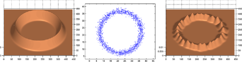
Figure 5: A thick circle density, a sample of size 2000 from this density and approximations using a mixture of 80 isotropic Gaussians.

We see that it successfully approximates the circle density with a relatively small number of components.

Appendix

Lemma 3

(I) Let $\tilde{\mu}$ be given by (29). Then $\bar{\mu}=(\tilde{\mu},0)\in\mathbb{R}^{M}$ is a minimizer in $\lambda\in\mathbb{R}^{M}$ of

$$g(\lambda)=-\frac{2}{n}\sum_{i=1}^{n}\mathsf{f}_{\lambda}(X_{i})+\|\mathsf{f}_{\lambda}\|^{2}+8Lr\sum_{k=1}^{M}|\lambda_{k}|$$

on the random event $\mathcal{B}$ defined in (30).

(II) Any two minimizers of $g(\lambda)$ have nonzero components in the same positions.

(I). Since $g$ is convex, by standard results in convex analysis, $\bar{\lambda}\in\mathbb{R}^{M}$ is a minimizer of $g$ if and only if $0\in D_{\bar{\lambda}}$ where $D_{\lambda}$ is the subdifferential of $g(\lambda)$:

$$D_{\lambda} = \Biggl{\{}w\in\mathbb{R}^{M}\dvtx w_{k}=-\frac{2}{n}\sum_{i=1}^{n}f_{k}(X_{i})+2\sum_{j=1}^{M}\lambda_{j}\langle f_{j},f_{k}\rangle+8rv_{k},$$

$$\hskip 154.2ptv_{k}\in V_{k}(\lambda_{k}),1\leq k\leq M\Biggr{\}},$$

where

$$V_{k}(\lambda_{k})=\cases{\{L\},&\quad if $\lambda_{k}>0$,\cr\{-L\},&\quad if $\lambda_{k}<0$,\cr[-L,L],&\quad if $\lambda_{k}=0$.}$$

Therefore, $\bar{\lambda}$ minimizes $g(\cdot)$ if and only if, for all $1\leq k\leq M$,

$$\frac{1}{n}\sum_{i=1}^{n}f_{k}(X_{i})-\sum_{j=1}^{M}\bar{\lambda}_{j}\langle f_{j},f_{k}\rangle = 4Lr\operatorname{sign}(\bar{\lambda}_{k})\qquad\mbox{if }\bar{\lambda}_{k}\neq 0,$$ (42)

$$\Biggl{|}\frac{1}{n}\sum_{i=1}^{n}f_{k}(X_{i})-\sum_{j=1}^{M}\bar{\lambda}_{j}\langle f_{j},f_{k}\rangle\Biggr{|} \leq 4Lr\qquad\mbox{if }\bar{\lambda}_{k}=0.$$ (43)

We now show that $\bar{\mu}=(\tilde{\mu},0)\in\mathbb{R}^{M}$ with $\tilde{\mu}$ given in (29) satisfies (42) and (43) on the event ${\mathcal{B}}$ and therefore is a minimizer of $g(\lambda)$ on this event. Indeed, since $\tilde{\mu}$ is a minimizer of the convex function $h(\mu)$ given in (28), the same convex analysis argument as above implies that

$$\frac{1}{n}\sum_{i=1}^{n}f_{k}(X_{i})-\sum_{j\in I^{*}}\tilde{\mu}_{j}\langle f_{j},f_{k}\rangle = 4Lr\operatorname{sign}(\tilde{\mu}_{k})\qquad\mbox{if }\tilde{\mu}_{k}\neq 0,k\in I^{*},$$

$$\Biggl{|}\frac{1}{n}\sum_{i=1}^{n}f_{k}(X_{i})-\sum_{j\in I^{*}}\tilde{\mu}_{j}\langle f_{j},f_{k}\rangle\Biggr{|} \leq 4Lr\qquad\mbox{if }\tilde{\mu}_{k}=0,k\in I^{*}.$$

Note that on the event ${\mathcal{B}}$ we also have

$$\Biggl{|}\frac{1}{n}\sum_{i=1}^{n}f_{k}(X_{i})-\sum_{j\in I^{*}}\tilde{\mu}_{j}\langle f_{j},f_{k}\rangle\Biggr{|}\leq 4Lr$$

$$\eqntext{\mbox{if }k\notin I^{*}\ (\mbox{for which }\bar{\mu}_{k}=0,\mbox{by construction}).}$$ (44)

Here $\bar{\mu}_{k}$ denotes the $k$th coordinate of $\bar{\mu}$. The above three displays and the fact that $\bar{\mu}_{k}=\tilde{\mu}_{k},k\in I^{*}$, show that $\bar{\mu}$ satisfies conditions (42) and (43) and is therefore a minimizer of $g(\lambda)$ on the event $\mathcal{B}$.

(II). We now prove the second assertion of the lemma. In view of (42), the index set $S$ of the nonzero components of any minimizer $\bar{\lambda}$ of $g(\lambda)$ satisfies

$$S=\Biggl{\{}k\in\{1,\ldots,M\}\dvtx\Biggl{|}\frac{1}{n}\sum_{i=1}^{n}f_{k}(X_{i})-\sum_{j=1}^{M}\bar{\lambda}_{j}\langle f_{j},f_{k}\rangle\Biggr{|}=4rL\Biggr{\}}.$$

Therefore, if for any two minimizers $\bar{\lambda}^{(1)}$ and $\bar{\lambda}^{(2)}$ of $g(\lambda)$ we have

$$\sum_{j=1}^{M}\bigl{(}\bar{\lambda}_{j}^{(1)}-\bar{\lambda}_{j}^{(2)}\bigr{)}\langle f_{j},f_{k}\rangle=0\qquad\mbox{for all }k,$$ (45)

then $S$ is the same for all minimizers of $g(\lambda)$.

Thus, it remains to show (45). We use simple properties of convex functions. First, we recall that the set of minima of a convex function is convex. Then, if $\bar{\lambda}^{(1)}$ and $\bar{\lambda}^{(2)}$ are two distinct points of minima, so is $\rho\bar{\lambda}^{(1)}+(1-\rho)\bar{\lambda}^{(2)}$, for any $0<\rho<1$. Rewrite this convex combination as $\bar{\lambda}^{(2)}+\rho\eta$, where $\eta=\bar{\lambda}^{(1)}-\bar{\lambda}^{(2)}$. Recall that the minimum value of any convex function is unique. Therefore, for any $0<\rho<1$, the value of $g(\lambda)$ at $\lambda=\bar{\lambda}^{2}+\rho\eta$ is equal to some constant $C$:

$$F(\rho) \triangleq -\frac{2}{n}\sum_{i=1}^{n}\sum_{j=1}^{M}\bigl{(}\bar{\lambda}^{(2)}_{j}+\rho\eta_{j}\bigr{)}f_{j}(X_{i})+\int\Biggl{(}\sum_{j=1}^{M}\bigl{(}\bar{\lambda}^{(2)}_{j}+\rho\eta_{j}\bigr{)}f_{j}(x)\Biggr{)}^{2}\,dx$$

$${}+8rL\sum_{j=1}^{M}\bigl{|}\bar{\lambda}^{(2)}_{j}+\rho\eta_{j}\bigr{|}=C.$$

By taking the derivative with respect to $\rho$ of $F(\rho)$, we obtain that, for all $0<\rho<1$,

$$F^{\prime}(\rho) = -\frac{2}{n}\sum_{i=1}^{n}\sum_{j=1}^{M}\eta_{j}f_{j}(X_{i})+8rL\sum_{j=1}^{M}\eta_{j}\operatorname{sign}\bigl{(}\bar{\lambda}^{(2)}_{j}+\rho\eta_{j}\bigr{)}$$

$${}+2{\int}\Biggl{(}\sum_{j=1}^{M}\bigl{(}\bar{\lambda}^{(2)}_{j}+\rho\eta_{j}\bigr{)}f_{j}(x)\Biggr{)}\Biggl{(}\sum_{j=1}^{M}\eta_{j}f_{j}(x)\Biggr{)}\,dx=0.$$

By continuity of $\rho\mapsto\bar{\lambda}^{(2)}_{j}+\rho\eta_{j}$, there exists an open interval in $(0,1)$ on which $\rho\mapsto\operatorname{sign}(\bar{\lambda}^{(2)}_{j}+\rho\eta_{j})$ is constant for all $j$. Therefore, on that interval,

$$F^{\prime}(\rho)=2\rho{\int}\Biggl{(}\sum_{j=1}^{M}\eta_{j}f_{j}(x)\Biggr{)}^{2}\,dx+C^{\prime},$$

where $C^{\prime}$ does not depend on $\rho$. This is compatible with $F^{\prime}(\rho)=0,\forall 0<\rho<1$, only if

$$\sum_{j=1}^{M}\eta_{j}f_{j}(x)=0\qquad\mbox{for all }x$$

and, therefore,

$$\sum_{j=1}^{M}\eta_{j}\langle f_{j},f_{k}\rangle=0\qquad\mbox{for all }k\in\{1,\ldots,M\},$$

which is the desired result. This completes the proof of the lemma.

References

- (1) Abramovich, F., Benjamini, Y., Donoho, D. L. and Johnstone, I. M. (2006). Adapting to unknown sparsity by controlling the false discovery rate. Ann. Statist. 34 584–653. \MR2281879
- (2) Biau, G. and Devroye, L. (2005). Density estimation by the penalized combinatorial method. J. Multivariate Anal. 94 196–208. \MR2161217
- (3) Biau, G., Cadre, B., Devroye, L. and Györfi, L. (2008). Strongly consistent model selection for densities. TEST 17 531–545. \MR2470097
- (4) Bickel, P. J., Ritov, Y. and Tsybakov, A. B. (2009). Simultaneous analysis of Lasso and Dantzig selector. Ann. Statist. 37 1705–1732. \MR2533469
- (5) Birgé, L. (2008). Model selection for density estimation with loss. Available at arXiv:0808.1416.
- (6) Birgé, L. and Massart, P. (1997). From model selection to adaptive estimation. In Festschrift for Lucien LeCam: Research Papers in Probability and Statistics (D. Pollard, E. Torgersen and G. Yang, eds.) 55–87. Springer, New York. \MR1462939
- (7) Bunea, F. (2004). Consistent covariate selection and post model selection inference in semiparametric regression. Ann. Statist. 32 898–927. \MR2065193
- (8) Bunea, F. (2008). Honest variable selection in linear and logistic models via and penalization. Electron. J. Stat. 2 1153–1194. \MR2461898
- (9) Bunea, F. (2008). Consistent selection via the Lasso for high dimensional approximating regression models. In Pushing the Limits of Contemporary Statistics: Contributions in Honor of Jayanta K. Ghosh (B. Clarke and S. Ghosal, eds.) 3 122–137. IMS, Beachwood, OH. \MR2459221
- (10) Bunea, F. and Barbu, A. (2009). Dimension reduction and variable selection in case control studies via regularized likelihood optimization. Electron. J. Stat. 3 1257–1287. \MR2566187
- (11) Bunea, F., Tsybakov, A. B. and Wegkamp, M. H. (2007). Aggregation for Gaussian regression. Ann. Statist. 35 1674–1697. \MR2351101
- (12) Bunea, F., Tsybakov, A. B. and Wegkamp, M. H. (2006). Aggregation and sparsity via -penalized least squares. In Proceedings of 19th Annual Conference on Learning Theory, COLT 2006. Lecture Notes in Artificial Intelligence 4005 379–391. Springer, Heidelberg. \MR2280619
- (13) Bunea, F., Tsybakov, A. B. and Wegkamp, M. H. (2007). Sparsity oracle inequalities for the Lasso. Electron. J. Stat. 1 169–194. \MR2312149
- (14) Bunea, F., Tsybakov, A. B. and Wegkamp, M. H. (2007). Sparse density estimation with penalties. In Learning Theory. Lecture Notes in Comput. Sci. 4539 530–544. Springer, Heidelberg. \MR2397610
- (15) Burden, R. L. and Faires, J. D. (2001). Numerical Analysis, 7th ed. Brooks/Cole, Pacific Grove, CA.
- (16) Chen, S., Donoho, D. and Saunders, M. (2001). Atomic decomposition by basis pursuit. SIAM Rev. 43 129–159. \MR1854649
- (17) Devroye, L. and Lugosi, G. (2000). Combinatorial Methods in Density Estimation. Springer, New York. \MR1843146
- (18) Donoho, D. L. (1995). Denoising via soft-thresholding. IEEE Trans. Inform. Theory 41 613–627. \MR1331258
- (19) Donoho, D. L., Elad, M. and Temlyakov, V. (2006). Stable recovery of sparse overcomplete representations in the presence of noise. IEEE Trans. Inform. Theory 52 6–18. \MR2237332
- (20) Friedman, J., Hastie, T., Hofling, H. and Tibshirani, R. (2007). Pathwise coordinate optimization. Ann. Appl. Statist. 1 302–332. \MR2415737
- (21) Friedman, J., Hastie, T. and Tibshirani, R. (2010). Regularization paths for generalized linear models via coordinate descent. Journal of Statistical Software 33 1.
- (22) Golubev, G. K. (1992). Nonparametric estimation of smooth probability densties in . Probl. Inf. Transm. 28 44–54. \MR1163140
- (23) Golubev, G. K. (2002). Reconstruction of sparse vectors in white Gaussian noise. Probl. Inf. Transm. 38 65–79. \MR2101314
- (24) Greenshtein, E. and Ritov, Y. (2004). Persistency in high dimensional linear predictor-selection and the virtue of over-parametrization. Bernoulli 10 971–988. \MR2108039
- (25) Härdle, W., Kerkyacharian, G., Picard, D. and Tsybakov, A. (1998). Wavelets, Approximation and Statistical Applications. Lecture Notes in Statistics 129. Springer, New York. \MR1618204
- (26) James, L., Priebe, C. and Marchette, D. (2001). Consistent estimation of mixture complexity. Ann. Statist. 29 1281–1296. \MR1873331
- (27) Kerkyacharian, G., Picard, D. and Tribouley, K. (1996). adaptive density estimation. Bernoulli 2 229–247. \MR1416864
- (28) Koltchinskii, V. (2005). Model selection and aggregation in sparse classification problems. Oberwolfach Reports 2 2663–2667.
- (29) Koltchinskii, V. (2009). Sparsity in penalized empirical risk minimization. Ann. Inst. H. Poincaré Probab. Statist. 45 7–57.
- (30) Loubes, J.-M. and van de Geer, S. A. (2002). Adaptive estimation in regression, using soft thresholding type penalties. Statist. Neerlandica 56 453–478.
- (31) Lounici, K. (2008). Sup-norm convergence rate and sign concentration property of Lasso and Dantzig estimators. Electron. J. Stat. 2 90–102. \MR2386087
- (32) Meinshausen, N. and Bühlmann, P. (2006). High-dimensional graphs and variable selection with the Lasso. Ann. Statist. 34 1436–1462. \MR2278363
- (33) Nemirovski, A. (2000). Topics in non-parametric statistics. In Lectures on Probability Theory and Statistics (Saint–Flour, 1998). Lecture Notes in Math. 1738 85–277. Springer, Berlin. \MR1775640
- (34) Press, W. H., Teukolsky, S. A., Vetterling, W. T. and Flannery, B. P. (2007). Numerical Recipes: The Art of Scientific Computing, 3rd ed. Cambridge Univ. Press, New York. \MR2371990
- (35) Rigollet, P. (2006). Inégalités d’oracle, agrégation et adaptation. Ph.D. thesis, Univ. Paris 6.
- (36) Rigollet, P. and Tsybakov, A. B. (2007). Linear and convex aggregation of density estimators. Math. Methods Statist. 16 260–280. \MR2356821
- (37) Rudemo, M. (1982). Empirical choice of histograms and kernel density estimators. Scand. J. Statist. 9 65–78. \MR0668683
- (38) Samarov, A. and Tsybakov, A. (2007). Aggregation of density estimators and dimension reduction. In Advances in Statistical Modeling and Inference. Essays in Honor of Kjell A. Doksum (V. Nair, ed.) 233–251. World Scientific, Singapore. \MR2416118
- (39) Tibshirani, R. (1996). Regression shrinkage and selection via the Lasso. J. Roy. Statist. Soc. Ser. B 58 267–288. \MR1379242
- (40) Tsybakov, A. B. (2003). Optimal rates of aggregation. In Proceedings of 16th Annual Conference on Learning Theory (COLT) and 7th Annual Workshop on Kernel Machines. Lecture Notes in Artificial Intelligence 2777. Springer, Heidelberg.
- (41) Vapnik, V. N. (1999). The Nature of Statistical Learning Theory (Information Science and Statistics). Springer, New York. \MR1367965
- (42) van de Geer, S. A. (2008). High dimensional generalized linear models and the Lasso. Ann. Statist. 26 225–287. \MR2396809
- (43) Wasserman, L. A. (2004). All of Statistics. Springer, New York. \MR2055670
- (44) Wegkamp, M. H. (1999). Quasi-universal bandwidth selection for kernel density estimators. Canad. J. Statist. 27 409–420. \MR1704442
- (45) Wegkamp, M. H. (2003). Model selection in nonparametric regression. Ann. Statist. 31 252–273. \MR1962506
- (46) Zhang, C. H. and Huang, J. (2008). The sparsity and biais of the Lasso selection in high-dimensional linear regression. Ann. Statist. 36 1567–1594. \MR2435448
- (47) Zhao, P. and Yu, B. (2007). On model selection consistency of Lasso. J. Mach. Learn. Res. 7 2541–2567. \MR2274449
- (48) Zou, H. (2006). The adaptive Lasso and its oracle properties. J. Amer. Statist. Assoc. 101 1418–1429. \MR2279469