On the use of continuous wavelet analysis for modal identification

Abstract

This paper reviews two different uses of the continuous wavelet transform for modal identification purposes. The properties of the wavelet transform, mainly energetic, allow to emphasize or filter the main information within measured signals and thus facilitate the modal parameter identification especially when mechanical systems exhibit modal coupling and/or relatively strong damping.

1 Introduction

The concept of wavelets in its present theoretical form was first introduced in the 1970s by Jean Morlet and the team of the Marseille Theoretical Physics Center in France working under the supervision of Alex Grossmann. Grossmann and Morlet[1] developed then the geometrical formalism of the continuous wavelet transform. Wavelets analysis has since become a popular tool for engineers. It is today used by electrical engineers engaged for processing and analyzing non-stationary signals and it has also found applications in audio and video compression. Less than ten years ago, some researchers proposed the use of wavelet analysis for modal identification purposes. However, use of wavelet transforms in real world mechanical engineering applications remains limited certainly due to widespread ignorance of their properties.

This paper presents two ways of using the continuous wavelet transform (CWT) for modal parameter identification according to the type of measured responses : free decay or frequency response functions (FRF).

In 1997, Staszewski [2] and Ruzzene [3] started to use wavelet analysis with the Morlet wavelet for the processing of free decay responses, but the identification of the mode shapes was not performed. Wavelet transform allows to reach the time variation of instantaneous amplitude and phase of each component within the signal and makes the identification procedure of modal parameters much easier. Compared to other mother wavelets, Morlet wavelet provides better energy localizing and higher frequency resolution but has a disadvantage: frequency-coordinate window shifts along frequency axis with scaling while other wavelet types only expands the window. To remedy it, Lardies et al. [4] and Slavic et al. [5] preferred the Gabor wavelet. Argoul et al. [6, 7] chose the Cauchy wavelet and Le et al. [8] established a complete modal identification procedure with improvements for numerical implementation, especially for a correct choice of the time-frequency localization. Edge effects are seen by all the authors and some attempts to reduce their negative influence on modal parameter identification are presented in [5], [8] and [9].

More recently, Staszewski [10], Bellizzi et al. [11] and Argoul et al. [6] adapted their identification procedure in order to process free responses of nonlinear systems. In [6], the authors proposed four instantaneous indicators, the discrepancy of which from linear case facilitates the detection and characterization of the non-linear behaviour of structures. In [11], an identification procedure of the coupled non-linear modes is proposed and tested on different types of non-linear elastic dynamic systems.

Typically, CWT is applied to time or spatial signals. Processing frequency signals is unusual, but a first application was proposed in [12] and [13]. Argoul showed in [12] that the weighted integral transform (WIT) previously introduced by Jézéquel et al. [14] for modal identification purposes can be expressed by means of a wavelet transform using a complex-valued mother wavelet close to the Cauchy wavelet. The WIT can be applied to either the ratio of the time derivative of the FRF over the FRF or the FRF itself. The representation with CWT provided a better understanding of the amplification effects of the WIT. When the FRF signal is strongly perturbed by noise, its derivative is hard to obtain; thus, Yin et al. [13] then proposed a slightly modified integral transform directly applied to the FRF and called the Singularities Analysis Function (SAF) of order $n$. It allows the influence of the FRF’s poles to be emphasized and direct estimation of the eigen frequencies, eigen modes, and modal damping ratios is performed from the study of the extrema of the WIT.

2 Theoretical background for the continuous wavelet analysis

A wavelet expansion uses translations and dilations of an analyzing function called the mother wavelet $\psi\in L^{1}(\mathbb{R})\cap L^{2}(\mathbb{R})$. For a continuous wavelet transform (CWT), the translation and dilation parameters: $b$ and $a$ respectively, vary continuously. In other words, the CWT uses shifted and scaled copies of $\psi(x)$ : $\psi_{b,a}(x)=\frac{1}{a}\psi(\frac{x-b}{a})$ whose $L^{1}(\mathbb{R})$ norms ($\left\|.\right\|_{1}$) are independent of $a$. In the following, $\psi(x)$ is assumed to be a smooth function, whose modulus of Fourier transform is peaked at a particular frequency $\Omega_{0}$ called the ”central” frequency. The variable $x$ may represent either time or frequency; when necessary, the time and circular frequency variables will be referred to $t$ and to $\omega$ respectively. The CWT of a function $u(x)\in L^{2}(\mathbb{R})$ can then be defined by the inner product between $u(x)$ and $\psi_{b,a}(x)$

$$T_{\psi}[u](b,a)=\left\langle u,\psi_{b,a}\right\rangle=\frac{1}{a}\int_{-\infty}^{+\infty}u(x)\,\overline{\psi}\left(\frac{x-b}{a}\right)dx$$ (1)

where $\overline{\psi}(.)$ is the complex conjugate of $\psi(.)$. Using Parseval’s identity, Eq. (1) becomes

$$T_{\psi}[u](b,a)=\frac{1}{2\pi}\left\langle\widehat{u},\widehat{\psi}_{b,a}\right\rangle=\frac{1}{2\pi}\int_{-\infty}^{+\infty}\widehat{u}(\Omega)\,\overline{\widehat{\psi}}(a\Omega)\,e^{i\Omega b}\,d\Omega$$ (2)

where $\widehat{u}(\Omega)$, $\widehat{\psi}_{b,a}(\Omega)$ and $\widehat{\psi}(\Omega)$ are respectively the Fourier transform (FT) of $u(x)$, $\psi_{b,a}(x)$ and $\psi(x)$; for instance for $u(x)$ : $\widehat{u}(\Omega)=\int_{-\infty}^{+\infty}u(x)\,e^{-i\Omega x}dx$.

Moreover, when $\psi$ and $u$ are continuous and piece-wise differentiable, and $\dot{\psi}$ is square and absolutely integrable, and $\dot{u}$ is of finite energy, the CWT of $\dot{u}$ with $\psi$ is linked to the CWT of $u$ with $\dot{\psi}$ :

$$T_{\psi}[\dot{u}](b,a)=-\frac{1}{a}T_{\dot{\psi}}[u](b,a)$$

From [15], it can be seen that the CWT at point $(b,\Omega=\frac{\Omega_{\psi}}{a})$ picks up information about $u(x)$, mostly from the localization domain $D(b,\Omega=\frac{\Omega_{\psi}}{a})$ of the CWT, defined as

$$D(b,\Omega=\frac{\Omega_{\psi}}{a})=[b+ax_{\psi}-a\Delta x_{\psi},b+ax_{\psi}+a\Delta x_{\psi}\,]\times[\frac{\Omega_{\psi}}{a}-\frac{\Delta\Omega_{\psi}}{a}\,,\frac{\Omega_{\psi}}{a}+\frac{\Delta\Omega_{\psi}}{a}]$$ (3)

where $x_{\psi}$ and $\Delta x_{\psi}$ are called centre and radius of $\psi,$ stated in terms of root mean squares : $x_{\psi}=\frac{1}{\left\|\psi\right\|_{2}^{2}}\int_{-\infty}^{+\infty}x\,\,\left|\psi(x)\right|^{2}\,dx$ and
$\Delta x_{\psi}=\frac{1}{\left\|\psi\right\|_{2}}\sqrt{\int_{-\infty}^{+\infty}\left(x-x_{\psi}\right)^{2}\,\left|\psi(x)\right|^{2}\,dx}$, and similar definitions hold on for the frequency centre $\Omega_{\psi}$ and the radius $\Delta\Omega_{\psi}$ of $\widehat{\psi}$. The area of $D$ is constant and equal to four times the uncertainty : $4\Delta x_{\psi}\Delta\Omega_{\psi}=4\mu(\psi)$. The Heisenberg uncertainty principle states that this area has to be greater than $2$.

Referring to the conventional frequency analysis of constant-$Q$ filters, the parameter $Q$ defined as the ratio of the frequency centre $\Omega_{\psi}$ to the frequency bandwidth ($2\Delta\Omega_{\psi}$):

$$Q\,=\,\frac{\frac{\Omega_{\psi}}{a}}{2\frac{\Delta\Omega_{\psi}}{a}}\,=\,\frac{\Omega_{\psi}}{2\Delta\Omega_{\psi}},$$ (4)

is introduced in [8] to compare different mother wavelets and to characterize the quality of the CWT. $Q$ is independent of $a$.

The notion of spectral density can be easily extended to the CWT (see [16] for others properties such as linearity, admissibility and signal reconstruction, etc.). From the Parseval theorem applied to Eq. 2, it follows that

$$\int_{-\infty}^{+\infty}\left|T_{\psi}[u](b,a)\right|^{2}\,db=\frac{1}{2\pi}\int_{-\infty}^{+\infty}\left|\widehat{u}(k)\right|^{2}\,\left|\overline{\widehat{\psi}}(ak)\right|^{2}\,dk$$

and it leads to the ”energy conservation” property of the CWT expressing that if $u\in L^{2}(\mathbb{R})$, then $T_{\psi}\in L^{2}(\mathbb{R\times R}_{+}^{\ast},db\frac{da}{a})$, and $\left\|T_{\psi}[u]\right\|^{2}=C_{\psi}\,\left\|u\right\|^{2}=\frac{C_{\psi}}{2\,\pi}\left\|\widehat{u}\right\|^{2}$. Finally, after changing the integration variable: $a=\frac{\Omega_{0}}{\Omega}$ and because $\widehat{u}(\Omega)$ is hermitian ($u(x)$ being real valued), one gets

$$\int_{0}^{+\infty}\int_{-\infty}^{+\infty}\left|T_{\psi}[u](b,\frac{\Omega_{o}}{\Omega})\right|^{2}db\frac{d\Omega}{\Omega}=\frac{C_{\psi}}{\,\pi}\int_{0}^{+\infty}\left|\widehat{u}(\Omega)\right|^{2}d\Omega$$ (5)

where $C_{\psi}=\int_{-\infty}^{+\infty}$ $\frac{\left|\widehat{\psi}(\omega)\right|^{2}}{\omega}d\omega<\infty$.

This allows to define a local wavelet spectrum: $E_{u,CWT}(\Omega,b)=\frac{1}{2C_{\psi}\,\Omega}\left|T_{\psi}[u](b,\frac{\Omega_{o}}{\Omega})\right|^{2}$ and a mean wavelet spectrum: $E_{u,CWT}(\Omega)=$ $\int_{-\infty}^{+\infty}E_{u,CWT}(\Omega,b)db$; and Eq. 5 can be rewritten: $\int_{0}^{+\infty}\left[E_{u,CWT}(\Omega)-\frac{1}{2\pi}\left|\widehat{u}(\Omega)\right|^{2}\right]\,d\Omega=0$.

When the mother wavelet $\psi$ is progressive (i.e. it belongs to the complex Hardy space $\widehat{\psi}(\Omega)=0:\mbox{for}:\Omega\leq 0$), the CWT of a real-valued signal $u$ is related to the CWT of its analytical signal $Z_{u}$ (see. [16])

$$T_{\psi}[u](b,a)=\frac{1}{2}T_{\psi}[Z_{u}](b,a)$$ (6)

From 3, the CWT has sharp frequency localization at low frequencies, and sharp time localization at high frequencies. Thanks to a set of mother wavelets depending on one(two) parameter(s), the desired time or frequency localization can be yet obtained by modifying its(their) value(s). In [8], two complex valued mother wavelets were analyzed : Gabor and Cauchy. Morlet wavelet is a complex sine wave localized with a Gaussian envelope and the Gabor wavelet function is a modified Morlet wavelet with a parameter controlling its shape. Cauchy wavelet $\psi_{n}$ of $n$ order for $n\geq 1$, is defined by:

$$\psi_{n}(x)=\left(\frac{i}{x+i}\right)^{n+1}=\left(\frac{1}{1-ix}\right)^{n+1}=\left[\frac{1}{\sqrt{x^{2}+1}}\right]^{n+1}e^{i\,(n+1)Arctg(x)}.$$ (7)

The main characteristics of $\psi_{n}(x)$ follow: its FT: $\widehat{\psi}_{n}(\Omega)=\frac{2\pi\Omega^{n}e^{-\Omega}}{n!}\,\Theta(\Omega)$ where $\Theta(\Omega)$ is the Heaviside function ($\psi_{n}$ is progressive), its central frequency: $\Omega_{0_{n}}=n$, its L2 norm: $\left\|\psi_{n}\right\|_{2}^{2}=\frac{(2n)!}{2^{2n}(n!)^{2}}\pi$, its x- and frequency centres: $x_{\psi}=0$ and $\Omega_{\psi}=n+\frac{1}{2}$, its radius: $\Delta x_{\psi}=\sqrt{\frac{1}{2n-1}}$, its frequency radius: $\Delta\Omega_{\psi}=\frac{\sqrt{2n+1}}{2}$, its uncertainty: $\mu_{\psi}=\frac{1}{2}\sqrt{1+\frac{2}{2n-1}}$, its quality factor: $Q=\frac{n+\frac{1}{2}}{\sqrt{2n+1}}$ and its admissibility factor: $C_{\psi}=4\pi^{2}\frac{1}{2^{2n}}\frac{(2n-1)!}{(n!)^{2}}=\frac{2\pi}{n}\left\|\psi_{n}\right\|_{2}^{2}$. The use of the Cauchy wavelet is legitimate when $Q$ is less than $5/\sqrt{2}$; as $Q$ increases, both wavelets give close results, a little better with Morlet wavelet due to its excellent time-frequency localization, and behave similarly in the both time and frequency domains when $Q$ tends toward infinity.

Some numerical and practical aspects for the computation of the CWT are detailed in [8], especially when applied to signals with time bounded support. Let us note $D_{u}=\left[0,L\right]\times\left[0,2\pi f_{Nyq}\right]$ the validity domain of the discretized signal in the $(b,\Omega)$ plane where $f_{Nyq}$ is the Nyquist frequency ($f_{Nyq}=\frac{1}{2T}$ with sampling period $T$). The edge-effect problem due to the finite length ($L$) and to the discretization of measured data record and to the nature of the CWT (convolution product) is tackled. An extended domain $D_{ext}(b,\Omega)\supset D(b,\Omega)$ where $\Omega=\frac{\Omega_{\psi}}{a})$, is then proposed to take into account the decreasing properties of $\psi$ and $\widehat{\psi}$ by introducing two real positive coefficients $c_{x}$ and $c_{\Omega}$: ${\footnotesize D_{ext}(b,\Omega=\frac{\Omega_{\psi}}{a})=[b+ax_{\psi}-a\,c_{x}\Delta x_{\psi},b+ax_{\psi}+ac_{x}\Delta x_{\psi}\,]\times[\frac{\Omega_{\psi}}{a}-c_{\Omega}\frac{\Delta\Omega_{\psi}}{a}}$ , ${\footnotesize\frac{\Omega_{\psi}}{a}+c_{\Omega}\frac{\Delta\Omega_{\psi}}{a}]}$. Forcing $D_{ext}$ to be included into $D_{u}$ leads the authors to define a region in the $(b,\Omega)$ plane where the edge effect can be neglected; this region is delimited by two hyperbolae whose equations are: $\Omega=\frac{2}{b}c_{x}Q\mu_{\psi}$ and $\Omega=\frac{2}{L-b}c_{x}Q\mu_{\psi}$ and two horizontal lines whose equations are: $\Omega=0$ and $\Omega=\frac{2\pi f_{Nyq}}{1+c_{\Omega}\frac{1}{2Q}}$. Let us consider a frequency $\Omega_{j}$ for which $\widehat{u}(\Omega)$ exhibits a peak and introduce a frequency discrepancy $d\Omega_{j}$ (for example, the distance between two successive peaks of $\widehat{u}(\Omega)$). From the intersection of the two hyperbolae at the point $(b={\footnotesize\frac{L}{2}},\Omega={\footnotesize\Omega_{j}})$ and by imposing the frequency localization along the straight line: $a={\footnotesize\frac{\Omega_{0}}{\Omega_{j}}}$, to be included into $\left[\Omega_{j}-d\Omega_{j},\Omega_{j}+d\Omega_{j}\right]$, some upper and lower bounds are found for $Q$: $c_{\Omega}\frac{\Omega_{j}}{2d\Omega_{j}}$ $\leq Q\leq\frac{L\,\Omega_{j}}{2c_{x}}$ and finally, the authors proposed $c_{x}=c_{\Omega}\simeq 5$.

3 Modal analysis and modal identification with CWT

Experimental identification of structural dynamics models is usually based on the modal analysis approach. One basic assumption underlying modal analysis is that the behaviour of the structure is linear and time invariant during the test. Modal analysis and identification involve the theory of linear time-invariant conservative and non-conservative dynamical systems. In this theory, the normal modes are of fundamental importance because they allow to uncouple the governing equations of motion. Also, they can be used to evaluate the free or forced dynamic responses for arbitrary sets of initial conditions. Modal analysis of a structure is performed by making use of the principle of linear superposition that expresses the system response as a sum of modal responses.

For linear MDOF systems with $N$ degrees of freedom, the transfer function $\mathbb{H}_{ij}(p)$ of receptance type is defined as the Laplace transform of the displacement at point $j$  to the impulse unit applied at point $i$ and it can be expressed as a sum of simple rational fractions

$$\mathbb{H}_{ij}(p)=\sum_{r=1}^{N}\left(\frac{\left(A_{r}\right)_{ij}}{p-p_{r}}+\frac{\left(\overline{A_{r}}\right)_{ij}}{p-\overline{p_{r}}}\right)$$ (8)

where $\left(\overline{A_{r}}\right)_{ij}$ and $\overline{p_{r}}$ are respectively the conjugate of the residues $\left(A_{r}\right)_{ij}$ and of the poles $p_{r}$ of $\mathbb{H}_{ij}(p)$. When the system is stable, $p_{r}=-\xi_{r}\,\omega_{r}+i\widetilde{\omega}_{r}$ where $\omega_{r}$, $\widetilde{\omega}_{r}$ are the undamped and the damped vibration angular frequencies and $\xi_{r}$ is the damping ratio for the mode $r$. $\left(A_{r}\right)_{ij}$ can also be expressed from the complex modes $\chi_{r}$ by $\left(A_{r}\right)_{ij}=\frac{\left(\chi_{r}\right)_{i}\,\left(\chi_{r}\right)_{j}}{\gamma_{r}}$ where $\gamma_{r}=\chi_{r}^{T}\underline{\underline{C}}\chi_{r}+2p_{r}\chi_{r}^{T}\underline{\underline{M}}\chi_{r}$, $\underline{\underline{M}}$ and $\underline{\underline{C}}$ being respectively the mass and viscous damping matrices. Moreover, the FRF of receptance type $H_{ij}(\omega)$ can be usually related to $\mathbb{H}_{ij}(p)$ by: $H_{ij}(\omega)=\mathbb{H}_{ij}(p=i\omega)$, leading to

$$H_{ij}(\omega)=\sum_{r=1}^{N}\left(\frac{-i\left(A_{r}\right)_{ij}}{\left(\omega-\widetilde{\omega}_{r}\right)-i\xi_{r}\,\omega_{r}}+\frac{-i\left(\overline{A_{r}}\right)_{ij}}{\left(\omega+\widetilde{\omega}_{r}\right)-i\xi_{r}\,\omega_{r}}\right)$$ (9)

The free responses at point $j$ in terms of displacements $u_{j}^{{}_{(free)}}(t)$ can be expressed according to the modal basis of complex modes: $\chi_{jr}=\eta_{jr}+i\,\kappa_{jr}$ ($r$ being the mode number, $1\leq r\leq N$)

$$u_{j}^{{}_{(free)}}(t)=\sum_{r=1}^{N}A_{rj}(t)\cos\left(\Phi_{rj}(t)\right)$$ (10)

where $A_{rj}(t)=\left|\chi_{jr}\right|\rho_{r}\,e^{-\xi_{r}\omega_{r}t}$ and $\Phi_{rj}(t)=\widetilde{\omega}_{r}t-\varphi_{r}+\arctan\left(\frac{\kappa_{jr}}{\eta_{jr}}\right)$. $\rho_{r}$ and $\varphi_{r}$ are defined from initial displacement and velocity of mode $r$ (cf. [17]).

In the case of proportional viscous damping (Basile assumption), introducing the real eigenvectors $\Psi_{r}$ of mode $r$ for the associated conservative system, and replacing the residues $\left(A_{r}\right)_{ij}$ with $\frac{\left(\Psi_{r}\right)_{i}\,\left(\Psi_{r}\right)_{j}}{2i\,\widetilde{\omega}_{r}m_{r}}$ in Eq. 9 lead to

$$H_{ij}(\omega)=\sum_{r=1}^{N}\frac{\left(\Psi_{r}\right)_{i}\,\left(\Psi_{r}\right)_{j}}{m_{r}\left(\omega_{r}^{2}-\omega^{2}+2i\,\xi_{r}\,\omega_{r}\omega\right)}$$ (11)

Moreover, in Eq. 10, $\kappa_{jr}=0$; thus $\left|\chi_{jr}\right|$ can be replaced by $\left|\left(\Psi_{r}\right)_{j}\right|$ and the term $\arctan\left(\frac{\kappa_{jr}}{\eta_{jr}}\right)$ can be equal to $0$ or $\pi$ according to the sign of the real part $\eta_{jr}$.

3.1 Modal identification using free decay responses

The processed signals $u_{j}^{{}_{(free)}}(t)$, whose expression is given in Eq. 10, can be considered under the assumption of weak damping ($\xi_{r}\ll\frac{1}{\sqrt{2}}$), as a sum of $N$ modal components: $A_{rj}(t)\,\cos(\Phi_{rj}(t))$ consisting in asymptotic signals. The approximation of asymptotic signal means that the oscillations resulting from the phase term: $\Phi_{rj}(t)$ are much faster than the variation coming from the amplitude term: $A_{rj}(t)$; it entails that the analytical signal associated with $A_{rj}(t)\,e^{i\Phi_{rj}(t)}$ can be approximated by: $A_{rj}(t)\,e^{i\Phi_{rj}(t)}$. Therefore, Eq. (6) and the linearity of the CWT entail that: $T_{\psi}[u_{j}^{{}_{(free)}}](b,a)=\frac{1}{2}\sum_{r=1}^{N}T_{\psi}[A_{rj}(t)\,e^{i\Phi_{rj}(t)}](b,a)$. Taking the Taylor expansion of each amplitude term of this sum, it follows that

$$T_{\psi}[u_{j}^{{}_{(free)}}](b,a)=\frac{1}{2}\sum_{r=1}^{N}\left(A_{rj}(b)\,e^{i\Phi_{rj}(b)}\,\overline{\widehat{\psi}(a\,\widetilde{\omega}_{r})}+R_{rj}(b,a)\right).$$ (12)

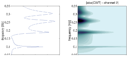
Figure 1: Modulus of FT and of the CWT for the 4DoF system ($Q=18$)

Assuming that each $R_{rj}(b,a)$ is small enough to be neglected, $\left|T_{\psi}[u_{j}^{{}_{(free)}}](b,a)\right|$ is peaked in the $(b,a)$ plane near straight lines of equation: $a=\frac{\Omega_{0}}{\Phi_{rj}^{\prime}(b)}=\frac{\Omega_{0}}{\widetilde{\omega}_{r}}$. When each modal pseudo-pulsation $\widetilde{\omega}_{r}$ is far enough from the others, this straight line’s equation easily provides an approximation of $\widetilde{\omega}_{r}$. Eq. 12 implies that the CWT of asymptotic signals has a tendency to concentrate near a series of curves in the time-frequency plane called ridges, which are directly linked to the amplitude and phase of each component of the measured signal. In [8], a complete modal identification procedure for natural frequencies, viscous damping ratios and mode shapes, is given in the case of viscous proportional damping and applied to a numerical case consisting in the free decay responses of a mass-spring-damper system with four degrees of freedom (4-DoF). The procedure is applied here to the free responses of a 4-DoF system whose natural frequencies are: $f_{1}=0.0984$ Hz, $f_{2}=0.1871$ Hz, $f_{3}=0.2575$ Hz and $f_{4}=0.3027$ Hz and modal damping ratios: $\xi_{1}=0.0124$, $\xi_{2}=0.0235$, $\xi_{3}=0.0324$, $\xi_{4}=0.0380$. Fig. 1 shows the FT and the CWT of the displacement of the second mass for which the four eigenfrequencies are clearly visible. Fig. 2 presents for the third mode and for the four masses, the modulus of the CWT and its logarithm that will allow to estimate the value of the damping ratio $\xi_{3}$ (cf. [8]). The edge effect is delimited by two hyperbolae in the time frequency plane; $Q$ being chosen to $20$ ($15.3\leq Q\leq 43.1$). Identified values are very close to the exact ones and identification errors are negligible inside the domain $D_{ext}$. This procedure was also applied in [7] to a set of accelerometric responses of modern buildings submitted to non destructive shocks. From the CWT of measured responses, the ridge and the corresponding amplitude and phase terms for the two first modes were extracted. For the first instantaneous frequency $\widetilde{\omega}_{1}$, the processing revealed a slight increase of $\widetilde{\omega}_{1}$ just after the shock. The origin of this non linear effect was attributed to the non-linear behaviour of the soil-structure interaction. Other preliminary results can be found in [6] where instantaneous indicators based on CWT are computed from the accelerometric responses of a non-linear beam to an impact force. A Duffing non-linearity effect was then identified thanks to the first and the super-harmonic components.

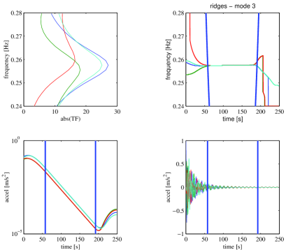
Figure 2: Modulus of FT and of CWT around the 3rd mode for all channels. Logarithm of the modulus of the CWT ($L=250$s, $T=0.175$s, $c_{t}=c_{\Omega}=4.7$, $Q=20$).

3.2 Modal identification using FRF functions

The first definition of the SAF of order $n$ ($n\in\mathbb{N}$) uses the derivative of a transfer function $\mathbb{H}(p)$ of the linear mechanical system, where $p=a+ib$ :

$$\mathbf{H}_{n}(b,a)=(-1)^{n}2\,\pi\,a^{\frac{n+1}{2}}\frac{d^{n}}{dp^{n}}\left\{\mathbb{H}(p)\right\}$$ (13)

$\mathbf{H}_{n}(b,a)$ can also be expressed as the FT of the impulse response function $h(t)$ filtered by: $2\pi a^{\frac{n+1}{2}}t^{n}e^{-at}\Theta(t)$ where $\Theta(t)$ is the Heaviside function :

$$\mathbf{H}_{n}(b,a)=2\pi\,a^{\frac{n+1}{2}}\int_{\mathbb{R}^{+}}t^{n}e^{-at}\,h(t)\,e^{-ibt}\,dt$$ (14)

Finally, $\mathbf{H}_{n}(b,a)$ is equal to the CWT of the FRF $H(\omega)$ with a mother wavelet being the conjugate of the Cauchy wavelet of order $n$ multiplied by $\frac{n!}{a^{\frac{n-1}{2}}}$ :

$$\mathbf{H}_{n}(b,a)=\frac{n!}{a^{\frac{n+1}{2}}}T_{\overline{\psi}_{n}}[H](b,a)=\frac{n!}{a^{\frac{n+1}{2}}}\int_{\mathbb{R}}H(\omega)\psi_{n}\left(\frac{\omega-b}{a}\right)\,d\omega$$ (15)

Let us now consider a transfer function restricted to only one term $F_{\lambda,\omega_{0}}(\omega)$ of the sum given in (9) and perturbed by a Gaussian white noise $n(\omega)$ so that : $H(\omega)=F_{\lambda,\omega_{0}}(\omega)+n(\omega)=\frac{-B\,i}{\left(\omega-\omega_{0}\right)-i\lambda}+n(\omega)$. Let us introduce the coefficient $\rho^{2}$ defined as the ratio of the square absolute value of the CWT of the pure signal upon the common variance of the CWT of the noise itself: $\rho^{2}=\frac{\left|T_{\psi}[H](b,a)\right|^{2}}{E\left\{\left|T_{\psi}[n](b,a)\right|^{2}\right\}}=\frac{\left|\left\langle F_{\lambda,\omega_{0}}\,,\,\psi_{b,a}\right\rangle\right|^{2}}{E\left\{\left|\left\langle n\,,\,\psi_{b,a}\right\rangle\right|^{2}\right\}}$, it looks like a signal to noise ratio.

The use of the Cauchy-Schwarz inequality gives that : $\rho^{2}\leq\left\|F_{\lambda,\omega_{0}}\right\|^{2}$ and the maximum of $\rho^{2}$ is reached for $(b,a)=(\omega_{0},\lambda)$ when $\psi_{b,a}(\omega)=K\,F_{a,b}(\omega)=K\frac{-B\,i}{\left(\omega-b\right)-ia}$ where $K$ is a constant. In conclusion, $\psi(\omega)=K\,B\frac{-\,i}{\omega-i}=K\,B\,\overline{\psi}_{0}(\omega)$; the analyzing functions $\psi(\omega)$ which allow the minimization of the noise effect on the peaks of $\left|T_{\psi}[H](b,a)\right|$ are proportional to $\overline{\psi}_{0}(s)$ defined in Eq. 7.

The above definitions of the SAF of order $n$ ($n\in\mathbb{N}^{*}$) allow to better understand its effect when applied to discrete causal linear mechanical systems. In Eq. 13, the successive derivatives of a rational fraction make the degree of the denominator increase and cause an amplification of the pole’s effect. So, when Eq. 8 is introduced in Eq. 13, the SAF of order $n$ becomes

$$\mathbf{H}_{n}(b,a)=2\pi\,n!\,a^{\frac{n+1}{2}}\sum_{r=1}^{N}\left(\frac{A_{r}}{\left(a+ib-p_{r}\right)^{n+1}}+\frac{\overline{A_{r}}}{\left(a+ib-\overline{p_{r}}\right)^{n+1}}\right)$$ (16)

The absolute value of $\mathbf{H}_{n}(b,a)$ exhibits $2N$ maxima located symmetrically from the vertical axis in the phase plane. The effect of parameter $n$ is to facilitate the modal identification, especially when the structure has neighboring poles. As soon as $n$ is large enough, the coordinates ($b_{max},a_{max}$) of these $2N$ maxima allow the estimation of the real and imaginary parts, respectively $\Re\left\{p_{r}\right\}$ and $\Im\left\{p_{r}\right\}$, of each of the $2N$ conjugate poles of the system :

$$\Re\left\{p_{r}\right\}=-\xi_{r}\,\omega_{r}\approx-a_{\max_{r}}\,\,\,\,\,\,\ \ \ \,\,\,\,\,\,\,\text{and}\,\,\,\,\,\,\ \ \ \,\,\,\,\,\,\,\Im\left\{p_{r}\right\}=\widetilde{\omega}_{r}\approx b_{\max_{r}}$$ (17)

The residue $A_{r}$ can be then estimated from the complex valued amplitude of the extremum called $\mathbf{H}_{n}^{\max_{r}}=\mathbf{H}_{n}^{\max}(a_{\max_{r}},b_{\max_{r}})$

$$A_{r}\approx\frac{2^{n}\left(a_{\max_{r}}\right)^{\frac{n+1}{2}}}{\pi\,n!}\mathbf{H}_{n}^{\max_{r}}$$ (18)

As $n$ increases, the estimation of the extrema is better for signals without noise; but for noisy signals, noise effects are also increased. Recently, Yin et al. [18] proposed the use of analyzing wavelets which are the conjugate of Cauchy wavelets in which $n$ is replaced by a positive real number. Applications both to numerical and experimental data showed the efficiency of this technique using SAF [19]. It was applied to the FRFs obtained with H1 estimators, of a test structure designed and build by ONERA for the GARTEUR-SM-AG19 Group. This structure was made of two aluminum sub-structures simulating wings/drum and fuselage/tail. Finally, the results obtained with SAF were very similar to those obtained with the broadband MIMO modal identification techniques provided by the MATLAB toolbox IDRC.

In conclusion, the pre-processing of measured signals (free decay responses or FRFs) with CWT proved to be an efficient tool for modal identification.

References

- [1] Grossman A., Morlet J. (1985) Decompositions of functions into wavelets of constant shape and related transforms, L. Streit, ed., World Scientific, Singapore, 135-165
- [2] Staszewski W.J. (1997) Identification of damping in MDOF systems using time-scale decomposition, Journal of Sound and Vibration, 203, 283-305
- [3] Ruzzene M., Fasana A., Garibaldi L., Piombo B. (1997) Natural frequencies and dampings identification using wavelet transform: application to real data, Mechanical Systems and Signal Processing, 11, 207-218
- [4] Lardies J., Ta M.N., Berthillier M. (2004) Modal parameter estimation based on the wavelet transform of output data, Archive of Applied Mechanics, 73, 718-733
- [5] Slavic J., Simonovski I., Boltezar M. (2003) Damping identification using a continuous wavelet transform: application to real data, Journal of Sound and Vibration, 262, 291-307
- [6] Argoul P., Le T-P. (2003) Instantaneous indicators of structural behaviour based on continuous Cauchy wavelet transform. Mechanical Systems and Signal Processing 17, 243-250
- [7] Argoul P., Le T-P. (2004) Wavelet analysis of transient signals in civil engineering. in M. Frémond & F. Maceri (Eds) Novel Approaches in Civil Engineering, Lecture Notes in Applied and Computational Mechanics, Springer-Verlag, 14, 311-318
- [8] Le T-P., Argoul P. (2004) Continuous wavelet transform for modal identification using free decay response, Journal of Sound and Vibration, 277, 73-100
- [9] Boltezar M., Slavic J. (2004) Enhancements to the continuous wavelet transform for damping identifications on short signals. Mechanical Systems and Signal Processing 18, 1065-1076
- [10] Staszewski W.J. (1998) Identification of non-linear systems using multi-scale ridges and skeletons of the wavelet transform, Journal of Sound and Vibration, 214, 639-658
- [11] Bellizzi S., Guillemain P., Kronland-Martinet R. (2001) Identification of coupled non-linear modes from free vibration using time-frequency representations, Journal of Sound and Vibration, 2432, 191-213
- [12] Argoul P. (1997) Linear dynamical identification : an integral transform seen as a complex wavelet transform. Meccanica, 32(3), 215-222
- [13] Yin H.P., Argoul P. (1999) Transformations intégrales et identification modale. C. R. Acad. Sci. Paris, Elsevier Paris, t. 327, Série II b, 777-783
- [14] Jézéquel L., Argoul P. (1986) A new integral transform for linear systems identification. Journal of Sound and Vibration, 111(2), 261-278
- [15] Chui C. K.( 1991) An introduction to Wavelets, (Charles K. Chui, Series Editor); San Diego: Academic Press
- [16] Carmona R., Hwang W-L., Torrésani B. (1998) Practical Time-Frequency Analysis. (Charles K. Chui, Series Editor); San Diego: Academic Press
- [17] Geradin M., Rixen D. (1996) Théorie des vibrations Application à la dynamique des structures, 2nd edition, Masson Paris (in french)
- [18] Yin H.P., Duhamel D., Argoul P. (2004) Natural frequencies and damping estimation using wavelet transform of a frequency response function, Journal of Sound and Vibration, 271, 999-1014
- [19] Argoul P., Guillermin B., Horchler A., Yin H-P. (1999) Integral transforms and modal identification in M.I. Friswell, J.E. Mottershead and A.W. Lees (Eds) Identification in Engineering Systems : Proceedings of the 2nd International Conference, Swansea, pp. 609-617