Phase separation transition in liquids and polymers induced by electric field gradients

Abstract

Spatially uniform electric fields have been used to induce instabilities in liquids and polymers, and to orient and deform ordered phases of block-copolymers. Here we discuss the demixing phase transition occurring in liquid mixtures when they are subject to spatially nonuniform fields. Above the critical value of potential, a phase-separation transition occurs, and two coexisting phases appear separated by a sharp interface. Analytical and numerical composition profiles are given, and the interface location as a function of charge or voltage is found. The possible influence of demixing on the stability of suspensions and on inter-colloid interaction is discussed.

I Introduction

Electric fields influence the structure and thermodynamic behavior of charged as well as neutral matter. Their effect is strong, they can be switched on or off, and they are easily scalable to the sub-micron regime LL1 . There are two main distinctions with respect to the field: spatially uniform vs. nonuniform fields. There are also two broad classes of material properties: pure dielectric vs. conducting media. All four combinations are relevant to phase transitions in liquid and polymer mixtures and to liquid-vapor coexistence in pure liquids.

Perfect dielectrics. The electrostatic energy of dielectric materials is given by the expression

$$F_{\rm es}=-\frac{1}{2}\int\varepsilon{\bf E}^{2}{\rm d}^{3}r$$ (1)

where $\varepsilon$ is the dielectric constant and ${\bf E}$ is the electric field. The negative sign before the integral is applicable to situations where the electric potential $\psi$ (${\bf E}=-\nabla\psi$) is given on the bounding surfaces; in cases where the charge is prescribed, ${\bf E}$ is given as a function of the displacement field ${\bf D}$, and the Legendre transform reverses the sign LL1 .

The phase-transition described below occurs in systems described by bistable free-energy functionals giving rise to a phase-diagram in the composition-temperature plane divided into two regions: homogeneous mixture and a phase-separated state. For concreteness, we consider the symmetric mixture free-energy density $f_{m}$ given by

$$\frac{v_{0}}{k_{B}T}f_{m}=$$ (2)

$$\left[\phi\log(\phi)+(1-\phi)\log(1-\phi)\right]+2k_{B}T_{c}\phi(1-\phi)$$

This free-energy is given in terms of the dimensionless composition $\phi$ ($0\leq\phi\leq 1$). In a binary mixture of two liquids 1 and 2, with dielectric constants $\varepsilon_{1}$ and $\varepsilon_{2}$, $\phi$ is the relative composition of (say) liquid 2. In A/B polymer blends, it is the relative volume fraction of polymer A, and similarly for an A/B diblock-copolymer melt. $v_{0}$ is a molecular volume, $k_{B}$ is the Boltzmann constant and $T_{c}$ is the critical temperature. In symmetric mixtures, the transition (binodal) temperature $T_{t}$ at a given composition is given by $df_{m}(T_{t},\phi)/d\phi=0$, that is, $T_{t}/T_{c}=2(2\phi-1)/\log(\phi/(1-\phi))$ doi . In the absence of electric field, the mixture is homogeneous if $T>T_{t}$, and unstable otherwise. The field-induced phase-transition discussed below does not depend on the exact form of $f_{m}$; it occurs also in a Landau series expansion of Eq. (2) around the critical composition $\phi_{c}$, and in other forms having a “double-well” shape.

The dielectric constant $\varepsilon$ depends on $\phi$ via a constitutive relation. A variation of $\phi$ from its critical value, $\phi_{c}$, induces a variation of $\varepsilon$ from the critical permittivity $\varepsilon_{c}$. When the composition deviation $\varphi\equiv\phi-\phi_{c}$ is small enough, $|\varphi|\ll 1$, the constitutive relation $\varepsilon(\phi)$ can be written as a Taylor series expansion to quadratic order:

$$\varepsilon(\phi)=\varepsilon_{c}+\Delta\varepsilon\varphi+\frac{1}{2}\varepsilon^{\prime\prime}\varphi^{2}$$ (3)

The “dielectric contrast” $\Delta\varepsilon$ is simply equal to $\varepsilon_{2}-\varepsilon_{1}$, if $\varepsilon^{\prime\prime}$ vanishes.

The electric field depends on the imposed external potentials or charges and on the local dielectric constant. Let us denote by ${\bf E}_{0}$ the electric field corresponding to the system with uniform composition $\phi_{c}$ everywhere. Composition changes in $\phi$ induce changes in $\varepsilon$, and since $\varepsilon$ and ${\bf E}$ are coupled via Laplace’s equation $\nabla(\varepsilon{\bf E})=0$, one has variations in electric field.

We may thus write to quadratic order in $\varphi$

$${\bf E}={\bf E}_{0}+{\bf E}_{1}\varphi+\frac{1}{2}{\bf E}_{2}\varphi^{2}~{}~{}.$$ (4)

Note that ${\bf E}_{0}$ is constant in space only inside a parallel-plate capacitor, or if the sources of the field are very far from the system under investigation. Clearly, even if ${\bf E}_{0}$ is uniform, composition variations lead to field nonuniformities.

One can expand the electrostatic energy density in Eq. (1) in powers of $\varphi$:

$$f_{\rm es} = const.-\left(\varepsilon_{c}{\bf E}_{0}\cdot{\bf E}_{1}+\frac{1}{2}\Delta\varepsilon{\bf E}_{0}^{2}\right)\varphi$$

$$- \frac{1}{2}\left(\frac{1}{2}\varepsilon^{\prime\prime}{\bf E}_{0}^{2}+\varepsilon_{c}{\bf E}_{1}^{2}+2\Delta\varepsilon{\bf E}_{0}\cdot{\bf E}_{1}+\varepsilon_{c}{\bf E}_{2}\cdot{\bf E}_{0}\right)\varphi^{2}$$

$$+ O(\varphi^{3})~{}~{}.$$

The unimportant constant corresponds to the electrostatic energy of the system with uniform composition, and it serves as a reference energy. If the field ${\bf E}_{0}$ is uniform in space, the two terms in linear order of $\varphi$ simply add a constant to the chemical potential, and therefore are inconsequential for the thermodynamic state of the system footnote .

Landau and Lifshitz showed that the existence of a $\varepsilon^{\prime\prime}\varphi^{2}$ term in Eq. (I) is responsible to a shift of the critical temperature $T_{c}$ LL1 ; tsori_rmp2009 . They found that $T_{c}$ is increased by $\Delta T_{c}$ given by

$$\Delta T_{c}=\frac{v_{0}\varepsilon^{\prime\prime}E_{0}^{2}}{2k_{B}}~{}~{}~{},$$ (6)

$T_{c}$ and the whole binodal curve close to the critical point are increased if $\varepsilon^{\prime\prime}>0$ (field-induced demixing) or decreased if $\varepsilon^{\prime\prime}<0$ (field-induced mixing). A similar expression exists for a pure liquid in coexistence with its vapor.

The experiments, starting with P. Debye and Kleboth debye_jcp1965 , are in contradiction with this prediction. Debye and Kleboth investigated the critical temperature of a Isooctane-Nitrobenzene mixture (relative permittivities $2.0$ and $34.2$, respectively) They observed reduction of $T_{c}$ by $15$ mK in a field of $4.5$ V/$\mu$m. Their measurements were later verified by Orzechowski orzech_chemphys1999 . Beaglehole worked with a Cyclohexane-Aniline mixture (relative permittivities $2$ and $7.8$, respectively), and he measured reduction of $T_{c}$ by as much as $80$ mK in a $0.3$ V/$\mu$m dc field beaglehole_jcp1981 . Early worked on the same mixture but in $1$ V/$\mu$m ac field, and found no change in $T_{c}$. He attributed the results of Beaglehole to spurious heating early_jcp1992 . Wirtz and Fuller performed similar experiments on n-hexane-Nitroethane mixture (relative permittivities $2$ and $19.7$, respectively), and found a reduction of $T_{c}$ by $20$ mK in a $5$ V/$\mu$m field wirtz_fuller_prl1993 . In all cases, $\varepsilon^{\prime\prime}$ was positive but still mixing was observed. In addition, the observed change in $T_{c}$ is quite small, typically in the $10$-$20$ mK range. The only exception is the work of Gordon and Reich reich_jpspp1979 . They worked on polymer mixtures of poly(vinyl methyl ether) (PVME)-polystyrene (PS) system (relative permittivities $2.15$ and $2.6$, respectively), and observed changes significantly larger than $1$ K. Their strong effect can be attributed to the large molecular weight of the polymer ($14,000$ – $30,000$ gr/mol) and to their reduced entropy compared to that of simple liquids.

One is inclined to explain the experimental findings by the second and third terms on the second line of Eq. (I) (proportional to $\varphi^{2}$). The third term is twice as large as the second one and opposite in sign, and the two sum to give a free energy contribution proportional to the dielectric contrast squared $+(\Delta\varepsilon)^{2}$. This is a free energy penalty for dielectric interfaces perpendicular to the external field. Indeed, these additional terms are responsible to the normal field instability in liquids tsori_rmp2009 , and to orientation of ordered phases (e.g. block-copolymers) in external fields ah_mm1991 ; ah_mm1993 ; ah_mm1994 ; russell_sci1996 ; muthu_jcp2001 ; onuki_mm1995 ; TA_mm2002 . In liquid mixtures they favor mixing (lowering of $T_{c}$).

II Mixtures of nonpolar liquids in fields gradients

Field gradients are general, and occur in all electrodes unless special care is taken to eliminate them (super-flat and parallel conducting surfaces). When mixtures of pure dielectric liquids are subjected to a spatially nonuniform field, the situation is very different. The direct coupling between field variations and composition fluctuations then leads to a dielectrophoretic force, depending on $\Delta\varepsilon$ in Eq. (3), which tends to “suck” the component with large $\varepsilon$ to regions with high electric field, as in the case of the well-known rise of a dielectric liquid in a capacitor LL1 .

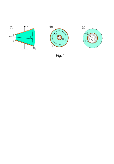
Figure 1: Three model systems where field gradients lead to demixing. (a) A wedge comprised of two flat electrodes with an opening angle $\beta$ and potential difference $V$. $R_{1}$ and $R_{2}$ are the minimal and maximal values of the distance $r$ from the imaginary meeting point. (b) A charged wire with radius $R_{1}$, or two concentric cylinders with radii $R_{1}$ and $R_{2}$. (c) A single charged colloid of radius $R_{1}$ and surface charge $\sigma$.

Statics
Three “canonical” geometries with electric field gradients are presented in Fig. 1. The first is the “wedge” capacitor, made up from two flat and nonparallel surfaces with potential difference $V$, and opening angle $\beta$. The electric field is then azimuthal, ${\bf E}(r)=V/(\beta r)\hat{\bf\theta}$, where $r$ is the distance from the imaginary meeting point of the surface. $r$ is bounded by the smallest and largest radii $R_{1}$ and $R_{2}$, respectively. The second model system consists of a charged wire of radius $R_{1}$, or two concentric metallic cylinders with radii $R_{1}$ and $R_{2}>R_{1}$. In this case the azimuthally-symmetric field is ${\bf E}(r)=\sigma R_{1}/(r\varepsilon(r))\hat{\bf r}$, where $\sigma$ is the charge per unit area on the inner cylinder. Lastly, for a charged spherical colloid of radius $R_{1}$ and surface charge $\sigma$, one readily finds the spherically-symmetric field to be ${\bf E}(r)=\sigma R_{1}/(r^{2}\varepsilon(r))\hat{\bf r}$.

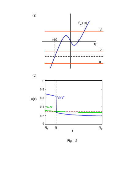
Figure 2: (a) Graphical solution to Eq. (8). Solid curve is $f_{m}^{\prime}(\varphi)$. Its roots are the transition (binodal) compositions. The intersection between $f_{m}^{\prime}(\varphi)$ and the horizontal dashed line gives the solution $\varphi(r)$ to Eq. (8). For voltages $V$ below the critical value $V^{*}$, the dashed line is bounded by lines a and b, corresponding to the the maximal and minimal values of the right-hand side of Eq. (8), giving rise to a continuous profile $\varphi(r)$. At $V>V^{*}$, line b is displaced to b’, and the intersection is at $\varphi<0$ for large $r$’s and at $\varphi>0$ at small $r$’s. (b) Qualitative composition profiles $\phi(r)$. Horizontal dashed line is the average composition $\phi_{0}$ in the absence of field. $\phi(r)$ varies smoothly when $V<V^{*}$, and has a sharp jump at $r=R$ when $V>V^{*}$.

In all three cases a general scenario occurs: when $T$ is above $T_{c}$, the composition profile $\phi({\bf r})$ is smooth, and its gradients increase as the charge on the objects increases. However, below $T_{c}$ the behavior is different – $\phi({\bf r})$ is smooth as long as the charge (voltage) is small, and becomes discontinuous when the charge (voltage) attains a critical value. At this charge, a sharp interface appears between the coexisting domains TTL_nature2004 ; KYL . As the charge further increases, the interface location and the compositions of the coexisting domains change.

To see this, consider the wedge capacitor, for which the electrostatic energy density is

$$f_{\rm es}=-\frac{1}{2}\left(\varepsilon_{c}+\Delta\varepsilon\varphi\right)\left(\frac{V}{\beta r}\right)^{2}$$ (7)

Note that we have used a linear constitutive relation. In uniform electric fields, such a linear relation would mean that the electrostatic energy is simply a constant independent of the composition profile. In addition, in the wedge geometry the electrostatic energy does not have a term proportional to $(\Delta\varepsilon)^{2}$ because the electric field is parallel to the dielectric interfaces (both are in the $\hat{\bf\theta}$ direction).

The equation that governs the composition profile $\varphi(r)$, derived from the Euler-Lagrange equation $\delta(f_{m}+f_{\rm es})/\delta\varphi=0$, is the following:

$$f_{m}^{\prime}(\varphi)=\frac{1}{2}\Delta\varepsilon\left(\frac{V}{\beta r}\right)^{2}+\mu~{}~{}.$$ (8)

Here $\mu$ is the chemical potential of the large reservoir at infinity. Note that Eq. (8) gives an analytical expression for $r$ as a function of $\varphi$.

The right hand side of the equation is independent of $\varphi$, and is indicated by the horizontal lines in Fig. 2 (a). Suppose the mixture composition in the absence of field corresponds to a point above and to the left of the binodal curve (homogeneous mixture). A graphical solution of the governing equation is obtained by the intersection of the horizontal line, whose location depends on the field, and therefore on $r$, with the curve $f_{m}^{\prime}(\varphi)$. If $T$ is above $T_{c}$, $f_{m}$ is convex, and therefore the intersection of the two curves changes smoothly as $r$ decreases ($E$ increases). The resulting composition profile is shown in Fig. 2 (b).

However, the situation is different below $T_{c}$: here $f_{m}^{\prime}(\varphi)$ behaves like $-\varphi+\varphi^{3}$. When the applied voltage is small enough such that the maximum value of the right-hand side of Eq. (8) occurs at line b of Fig. 2 (a), as one goes from large to small values of $r$ (increasing $E$), the composition increases, but $\varphi(r)$ is always continuous. There is a critical value of the voltage, $V^{*}$, where this is not true: above the critical potential, the maximum value of the horizontal line can be at b’ in the figure. Therefore, $\varphi$ increases with decreasing $r$ until, at a certain location $r=R$, there are three solutions. The middle one is an unstable while the other two are stable. At this point, the composition “jumps” between the two stable values and a discontinuity appears. At such voltages, the profiles are discontinuous and the coexistence between two distinct phases occurs.

Assuming that the jump in $\phi$ occurs at the binodal values, one obtains the stability criterion TTL_nature2004

$$\Delta T=\frac{v_{0}}{2k_{B}}\left|\frac{\Delta\varepsilon}{\phi_{c}-\phi_{0}}\right|E^{2}~{}~{}.$$ (9)

Here $E=V/(\beta R_{1})$ is the largest value of the field. A mixture of initial homogeneous composition $\phi_{0}$ is unstable and demixes into two coexisting domains under the given field if the temperature is below $T_{t}+\Delta T$, where $T_{t}(\phi_{0})$ is the zero-field transition (binodal) temperature at composition $\phi_{0}$. In contrast to uniform fields, where field variations result from composition variations, here field gradient are due to the non-flat geometry of electrodes. Hence, $\Delta T$ above is typically $2$-$100$ times larger than $\Delta T$ in uniform fields [Eq. (6)]. Note that similar demixing is also expected to occur in a rapidly rotating centrifuge. In that case $(\omega r)^{2}$ is the analogue of the spatially-dependent field $E^{2}$, where $r$ is the distance from the rotation axis and $\omega$ the angular frequency. The density difference $\Delta\rho\equiv\rho_{2}-\rho_{1}$ replaces the dielectric contrast $\Delta\varepsilon$ tsori_crphysique2007 .

Eq. (9) may be inverted to give the critical voltage for demixing $V^{*}$ as a function of $\phi_{0}$ and temperature. One finds that $V^{*}\propto(T-T_{t})^{1/2}$. In the experiments of the Leibler group, conducted using sharp “razor-blade” electrodes, the measured exponent was $0.7\pm 0.15$, larger than the value $1/2$ cited here. One may write the dimensionless potential as $U_{w}\equiv V\left[v_{0}\varepsilon_{0}/(4\beta^{2}k_{B}T_{c}R_{1}^{2})\right]^{1/2}$, where $\varepsilon_{0}$ is the vacuum permittivity. The critical value of $U_{w}$ for a closed wedge, $U_{w}^{*}$, is obtained by an approximation similar to that of Eq. (9), namely marcus_jcp2008

$$U_{w}^{*2}=\frac{v_{0}}{k_{B}T_{c}}\frac{\phi_{t}-\phi_{0}}{4|\Delta\varepsilon|/\varepsilon_{0}}\frac{d^{2}f_{m}(\phi_{t})}{d\phi^{2}}g(x)~{}~{},$$ (10)

where $\phi_{t}$ is the transition composition, $x=R_{2}/R_{1}$, and the dimensionless function $g$ is given by $g(x)=2(x^{2}-1)/(x^{2}-1-2\ln x)$.

Dynamics
The phase ordering dynamics of mixtures in electric field is quite different from the no-field case, since the electric field introduces a preferred direction and thus breaks the initial system symmetry. The phase transition studied here is even more difficult, because spatially nonuniform fields also break the translational symmetry.

In this phase transition, droplets nucleate everywhere, not only in regions of high electric field. As they grow, they move under the external force. The viscosity plays an important role, in addition to the field’s amplitude, location in the phase diagram and distance from the binodal, and dielectric constant mismatch $\Delta\varepsilon$. Clearly, the spatial dependence of the electric field means the initial destabilization and phase ordering dynamics are quite different from the well-studied normal-field instability in thin liquid films hermin1999 ; russell_steiner2000 ; russell2003 ; russel2003 ; tsori_rmp2009 and the regular coarsening dynamics onuki_book ; bray .

For salt-free mixtures, the starting point for the dynamics is the following set of equations onuki_pre2004 ; tanaka ; bray :

$$\frac{\partial\phi}{\partial t}+{\bf u}\cdot\nabla\phi = L\nabla^{2}\frac{\delta f}{\delta\phi}~{}~{},$$ (11)

$$\nabla\cdot(\varepsilon(\phi)\nabla\psi) = 0~{}~{},$$ (12)

$$\nabla\cdot{\bf u} = 0~{}~{},$$ (13)

$$\rho\left[\frac{\partial{\bf u}}{\partial t}+({\bf u}\cdot{\bf\nabla}){\bf u}\right] = \eta\nabla^{2}{\bf u}-\nabla P-\phi\nabla\frac{\delta f}{\delta\phi}~{}~{}.$$ (14)

${\bf u}$ is the velocity field corresponding to hydrodynamic flow and $\eta$ is the liquid viscosity. Equation (11) is a continuity equation for $\phi$, where $-L\nabla(\delta f/\delta\phi)$ is the diffusive current due to inhomogeneities of the chemical potential, and $L$ is the transport coefficient (assumed constant). Equation (12) is Laplace’s equation, Eq. (13) implies incompressible flow, and Eq. (14) is Navier-Stokes equation with a force term $-\phi\nabla\delta f/\delta\phi$ onuki_book ; bray . It should be noted that similar models have been proposed in the literature; the main differences here are the bistability of $f_{m}$ and the nonuniform fields derivable from the potential $\psi$. The presence of salt is naturally incorporated into the model by adding two continuity equations for the two ionic species, and by using Poisson’s equation instead of Laplace’s. As a starting point, we assume there is no net flow due to pressure gradients or moving solid surfaces – flow will be purely a result of the forces exerted by the electric field. In addition, the liquid viscosity $\eta$ is taken as a simple constant scalar, independent of mixture composition.

Since the equations are coupled and nonlinear, it is useful to first study the demixing in one of the geometries mentioned above (sphere, cylinder, or wedge). Consider, for example, the simplifications of the phase-ordering equations occurring in the system of concentric cylinders. In this annular capacitor, the no-flow conditions on the inner and outer cylinders lead to a vanishing flow velocity: ${\bf u}\equiv 0$ everywhere. One is therefore left with only a single equation to solve, $\partial\phi/\partial t=L\nabla^{2}\delta f/\delta\phi$. This equation can be viewed as a continuity equation $\partial\phi/\partial t=-\mathbf{\nabla}\cdot\mathbf{J}$, with a current density $J=-L\nabla\delta f/\delta\phi$. In a closed system, J vanishes at $R_{1}$ and $R_{2}$, and the integral $\int^{R_{2}}_{R_{1}}2\pi r\phi(r,t){\rm d}r$ is kept constant throughout the system dynamics. Gauss’s law readily gives the electric field in the concentric capacitor when the charge is given. In the explicit scheme we used, $\phi(t)$ is given by a successive summation of $-(\mathbf{\nabla}\cdot\mathbf{J})dt$, calculated for each time interval $dt$. The initial condition for the calculation was a homogeneous distribution $\phi_{0}$.

When the charge on the capacitor is larger than a threshold charge, we observe fast creation of a discontinuity near the inner cylinder which then starts to move outsides. The location of this front, separating the inner and outer regions, $R(t)$, is shown against time in Fig. 3 (a). In closed systems, $R$ cannot grow indefinitely, since mass conservation dictates an upper bound $R_{\rm max}$ given by

$$R_{\rm max}^{2}=\left(R_{2}^{2}-R_{1}^{2}\right)\phi_{0}+R_{1}^{2}~{}~{}.$$ (15)

In the numerical calculation, we find a match to an exponential relaxation with a single time constant $\tau$:

$$R(t)=R_{t=0}+(R_{\infty}-R_{t=0})(1-e^{-t/\tau})~{}~{}.$$ (16)

$R_{\infty}$ corresponds to the steady-state solution; it tends to $R_{\rm max}$ when the voltage or charge tend to infinity. The time constant $\tau$ depends on the external potential (or charge) and on the temperature and composition. Part (b) plots $\tau$ as a function of temperature for different average compositions. The calculations indicate faster dynamics (smaller $\tau$) when the average composition is farther from the critical value (large $|\phi_{0}-\phi_{c}|$) or when the cylinder’s charge is large, see Fig. 3 (b).

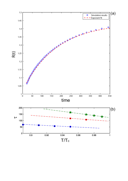
Figure 3: (a) Plot of the $R(t)$, the dynamics of front location between coexisting phases, for a mixture confined by two concentric cylinders when the charge on the inner cylinder is above the demixing threshold. $\phi_{0}=0.3$, $T/T_{c}=0.95$, and the dimensionless charge of the inner cylinder is $U_{c}=0.445$, where $U_{c}\equiv\sigma\left[v_{0}/(4\varepsilon_{0}k_{B}T_{c})\right]^{1/2}$, $\sigma$ is the charge per unit area of the cylinder, and $R_{1}$ is its radius. The exponential time constant $\tau$ in Eq. (16) is plotted in (b) for different values of $\phi_{0}$ and $U_{c}$. Blue circles: $\phi_{0}=0.2$, $U_{c}=0.252$. Green stars: $\phi_{0}=0.3$, $U_{c}=0.199$. Red squares: $\phi_{0}=0.3$, $U_{c}=0.252$. $R$ is scaled by $R_{1}$, and time is scaled by $Lk_{B}T/(v_{0}R_{1}^{2})$.

III Mixtures containing salt

Mixtures of polar liquids (e.g. aqueous solutions) contain some amount of charge carriers. In such mixtures, the physics is rich and quite different from the simple dielectric case. The most important feature is due to screening, occurring when dissociated ions accumulate at the charged surfaces. This means that the electric field is substantial only close to the surfaces, within the screening distance $\lambda$. Field gradients thus originate from both geometry and screening, and the phase transition depends on at least two lengths. The ionic screening therefore adds to the dielectrophoretic force which separates the liquids components from each other. Since screening is omni-present, phase-separation may occur even near parallel and flat charged surfaces, i.e. in one dimension. But ions have another effect besides increasing the dielectrophoretic force. Ions have in general different solubilities in the different liquids. As an ion drifts toward the electrode, it might “drag” with it the preferred liquid component onuki_jcp2004 ; onuki_pre2006 . Thus, the solubility introduces a force of electrophoretic origin, proportional to the ions’ charge.

We use the following free energy density to describe the system:

$$f = f_{m}(\phi)-\frac{1}{2}\varepsilon(\phi)\left(\nabla\psi\right)^{2}+\left(n^{+}-n^{-}\right)e\psi$$

$$+ k_{B}T\left[n^{+}\ln\left(v_{0}n^{+}\right)+n^{-}\ln\left(v_{0}n^{-}\right)\right]-\mu\phi$$

$$- \left(\Delta u^{+}n^{+}+\Delta u^{-}n^{-}\right)\phi-\lambda^{+}n^{+}-\lambda^{-}n^{-}+const.$$

The free energy depends on three fields: the electric potential $\psi({\bf r})$, and the two number densities of positive and negative ions: $n({\bf r})^{\pm}$. The new terms added here are the interaction of ions with the potential ($n^{\pm}\psi$) and the ideal-gas entropy of ions (logarithmic terms). In addition, the parameters $\Delta u^{+}$ and $\Delta u^{-}$ measure the affinity of the positive and negative ions toward the liquid-1 environment, respectively TL_pnas2007 . $\Delta u^{+}$, for example, measures how much a positive ions prefers liquid-2 environment over that of liquid 1. $\lambda^{\pm}$ and $\mu$ are the Lagrange multipliers (chemical potentials) of the positive and negative ions and liquid composition, respectively, and $e$ is the electron charge.

The free energy is extremized with respect to the fields $\phi$, $\psi$, and $n^{\pm}$:

$$\frac{\delta f}{\delta\phi} = \frac{\delta f_{m}}{\delta\phi}-\frac{1}{2}\frac{\delta\varepsilon}{\delta\phi}\left(\nabla\psi\right)^{2}-\Delta u^{+}n^{+}-\Delta u^{-}n^{-}-\mu=0$$

(18)

$$\frac{\delta f}{\delta\psi} = \nabla\left(\varepsilon(\phi)\nabla\psi\right)+e\left(n^{+}-n^{-}\right)=0$$ (19)

$$\frac{\delta f}{\delta n^{\pm}} = \pm e\psi+k_{B}T\left(\ln(v_{0}n^{\pm})+1\right)-\Delta u^{\pm}\phi-\lambda^{\pm}=0$$

in keeping with a fixed mixture and ion concentrations:

$$\mathcal{V}^{-1}\int\phi({\bf r}){\rm d}^{3}r=\phi_{0}$$ (21)

$$\mathcal{V}^{-1}\int n^{\pm}({\bf r}){\rm d}^{3}r=n_{0}$$ (22)

Here $\mathcal{V}$ is the total volume and $n_{0}$ the average ion concentration. The Poisson-Boltzmann equation is obtained from substitution of Eq. (LABEL:eq_gov_eq3) in the Poisson equation, Eq. (19).

Due to these forces, the phase transition is expected to be greatly enhanced compared to the no-ions case: it should occur at elevated temperature above the binodal, and lead to a very thin demixing layer around the charged object TL_pnas2007 . Consider a mixture in the semi-infinite space $x>0$ confined by one wall at $x=0$ charged at potential $V$. An approximate formula for the temperature below which a phase transition occurs, $T_{t}+\Delta T$, can be obtained by performing a first loop in a perturbative solution of the equations, namely using a uniform dielectric constant in Eqs. (19) and (LABEL:eq_gov_eq3) and substitution in Eq. (18). The expression for $\Delta T$ is then found to be TL_pnas2007 :

$$\frac{\Delta T}{T_{c}}=\left(\frac{|\Delta\varepsilon|}{\varepsilon_{c}}+\frac{\Delta u}{k_{B}T_{c}}\right)\frac{n_{0}v_{0}}{\phi_{0}-\phi_{c}}\exp\left(-\frac{eV}{k_{B}T_{c}}\right)$$ (23)

Here $\Delta u=|\Delta u^{\pm}|$. In most cases, $\Delta\varepsilon/\varepsilon_{c}\sim\Delta u/k_{B}T\sim 1$, and therefore the dielectrophoretic and solubility forces have the same magnitudes. The numerator $n_{0}v_{0}$ is quite small: if we take $v_{0}=8\times 10^{-27}$ m³ and average ion density $n_{0}=6\times 10^{19}$ m^-3 ($10^{-7}$M) we get $n_{0}v_{0}\simeq 5\times 10^{-7}$. However, $\Delta T$ is usually large. Even if we ignore the denominator $|\phi_{c}-\phi_{c}|^{-1}$, the exponential factor can be huge: if the surface potential is only $1$ Volt and $T_{c}$ is the room temperature, we get $eV/k_{B}T_{c}\simeq 40$. This shows us that demixing should be observed even if the surface potential $V$ or the charge density $n_{0}^{\pm}$ are much smaller.

We would like to note that for homogeneous dielectric liquids, the equation $\nabla(\varepsilon\nabla\psi)=0$ means that an increase of the potential on the bounding surfaces simply increases the potential $\psi$ proportionally, but that for ion-containing mixtures this is not true: due to the nonlinearity of the problem, increase of the external potential leads to a change in the whole distribution $\psi({\bf r})$. The composition difference between coexisting phases increases with $V$, and the front separating the domains may move to larger or smaller radii.

IV Conclusions

The steady-state and dynamics of phase transitions due to inhomogeneous electric field are discussed. In nonpolar mixtures, the composition profile of a mixture is given for three geometries with azimuthal or spherical symmetries. Above $T_{c}$, the profile is smooth, while below $T_{c}$ it becomes discontinuous if the surface charge or voltage exceed their critical values. The location of the front separating the two coexisting phases in equilibrium moves to larger values of $r$ as the charge or potential increase. In the restricted case shown here, the main feature of the dynamical process towards equilibrium is the exponential relaxation of the front location. The exponential time constant decreases when the potential is diminished or when the distance from the critical composition is reduced.

When salt is present, the phase transition is enhanced because ionic screening leads to a dielectrophoretic force. In addition, the ions’ solubility leads to a strong force of electrophoretic origin. Thus, the transition is g strengthened and should occur at virtually all temperatures above the binodal even at modest salt content. Our results nicely complement the recent studies by Onuki and co-workers on the solvation effects of ions in near critical mixtures onuki_epl1995 ; onuki_pre2004 ; onuki_jcp2004 ; onuki_pre2006 .

A similar phase transition was observed for a monolayer of surfactant mixture subject to an electric field emanating from a charged wire passing perpendicular to the monolayer KYL . The more polar surfactant was attracted to the wire when the field was applied, while the less polar surfactant was repelled. The effect observed was linear in electric field because (i) the dipoles were fixed and not induced, and (ii) they were confined to a plane and could not twist up-side-down when the field’s polarity was reversed.

We point out that when charged colloids are dispersed in aqueous solutions, a thin wetting layer could be formed due to field-induced demixing, depending on the average salt content, temperature, and colloid charge. According to Eq. (23), this demixing is quite favorable, and one needs not be very close to the binodal curve. This should have implications on colloidal aggregation beysens and on the interaction between charged surfaces in solution bechinger_nature2008 , because the electrostatically-induced capillary interaction between the surfaces is expected to be attractive.

References

- (1) L. D. Landau and E. M. Lifshitz: Elektrodinamika Sploshnykh Sred, Nauka, Moscow (1957) Ch. II, Sect. 18, problem 1.
- (2) M. Doi: Introduction to Polymer Physics, Oxford University Press, Oxford, UK (1996).
- (3) One may write as a sum: , where is the field’s component in the direction perpendicular to . If is uniform, it can be shown that is independent of , and hence .
- (4) Y. Tsori: Rev. Mod. Phys. (2009).
- (5) P. Debye and K. Kleboth: J. Chem. Phys. 42 (1965) 3155 (1965).
- (6) K. Orzechowski: Chem. Phys. 240 (1999) 275.
- (7) D. Beaglehole: J. Chem. Phys. 74 (1981) 5251.
- (8) M. D. Early: J. Chem. Phys. 96 (1992) 641.
- (9) D. Wirtz and G. G. Fuller: Phys. Rev. Lett. 71 (1993) 2236.
- (10) S. Reich and J. M. Gordon: J. Pol. Sci.: Pol. Phys. 17 (1979) 371.
- (11) K. Amundson, E. Helfand, D. D. Davis, X. Quan, S. S. Patel, and S. D. Smith: Macromolecules 24 (1991) 6546.
- (12) K. Amundson, E. Helfand, X. Quan, and S. D. Smith: Macromolecules 26 (1993) 2698.
- (13) K. Amundson, E. Helfand, X. Quan, S. D. Hudson, and S. D. Smith: Macromolecules 27 (1994) 6559.
- (14) T. L. Morkved, M. Lu, A. M. Urbas, E. E. Ehrichs, H. M. Jaeger, P. Mansky, and T. P. Russell: Science 273 (1996) 931.
- (15) B. Ashok and M. Muthukumar: J. Chem. Phys. 115 (2001) 1559.
- (16) A. Onuki and J. Fukuda: Macromolecules 28 (1995) 8788.
- (17) Y. Tsori and D. Andelman: Macromolecules 35 (2002) 5161.
- (18) A. Onuki: Europhys. Lett. 29 (1995) 611.
- (19) Y. Tsori, F. Tournilhac, and L. Leibler: Nature 430 (2004) 544.
- (20) K. Y. C. Lee, J. F. Klinger, and H. M. McConnell: Science 263 (1994) 655.
- (21) Y. Tsori and L. Leibler: C. R. Physique 8 (2007) 955.
- (22) G. Marcus, S. Samin, and Y. Tsori: J. Chem. Phys. 129 ( 2008) 061101.
- (23) S. Herminghaus: Phys. Rev. Lett. 83 (1999) 2359.
- (24) E. Schäffer, T. Thurn-Albrecht, T. P. Russell, and U. Steiner: Nature 403 (2000) 874.
- (25) M. D. Morariu, N. E. Voicu, E. Schäffer, Z. Lin, T. P. Russell, and U. Steiner: Nature Mater. 2 (2003) 48.
- (26) L. F. Pease and W. B. Russel: J. Chem. Phys. 118 (2003) 3790.
- (27) A. Onuki: Phase Transition Dynamics, Cambridge University Press (2002).
- (28) A. J. Bray: Adv. Phys. 51 (2002) 481.
- (29) T. Imaeda, A. Furukawa, and A. Onuki: Phys. Rev. E 70 (2004) 051503.
- (30) H. Tanaka: J. Phys.: Condens. Matter 12 (2000) R207.
- (31) A. Onuki and H. Kitamura: J. Chem. Phys. 121 (2004) 3143.
- (32) A. Onuki: Phys. Rev. E 73 (2006) 021506.
- (33) Y. Tsori and L. Leibler: Proc. Natl. Acad. Sci. (USA) 104 (2007) 7348.
- (34) D. Beysens and T. Narayanan: J. Stat. Phys. 95 (1999) 997.
- (35) C. Hertlein, L. Helden, A. Gambassi, S. Dietrich, and C. Bechinger: Nature 451 (2008) 172.