The complex, variable near-Infrared extinction towards the Nuclear Bulge

Abstract

Using deep $J$, $H$ and $K_{\rm S}$-band observations, we have studied the near-infrared extinction of the Nuclear Bulge and we find significant, complex variations on small physical scales. We have applied a new variable near-infrared colour excess method, V-NICE, to measure the extinction; this method allows for variation in both the extinction law parameter $\alpha$ and the degree of absolute extinction on very small physical scales. We see significant variation in both these parameters on scales of $5\arcsec$. In our observed fields, representing a random sample of sight lines to the Nuclear Bulge, we measure $\alpha$ to be $2.64\pm 0.52$, compared to the canonical “universal” value of 2. Our measured levels of $A_{K_{\rm S}}$ are similar to previously measured results ($1\leq A_{K_{\rm S}}\leq 4.5$); however, the steeper extinction law results in higher values for $A_{J}$ ($4.5\leq A_{J}\leq 10$) and $A_{H}$ ($1.5\leq A_{H}\leq 6.5$). Only when the extinction law is allowed to vary on the smallest scales can we recover self-consistent measures of the absolute extinction at each wavelength, allowing accurate reddening corrections for field star photometry in the Nuclear Bulge. The steeper extinction law slope also suggests that previous conversions of near-infrared extinction to $A_{V}$ may need to be reconsidered. Finally, we find that the measured values of extinction are significantly dependent on the filter transmission functions of the instrument used to obtain the data. This effect must be taken into account when combining or comparing data from different instruments.

1 Introduction

Study of the structure and stellar content of the Nuclear Bulge is extremely difficult as it is one of the most highly obscured regions of the Galaxy. The Nuclear Bulge is estimated to contain a narrow layer of molecular hydrogen throughout its extent with scale height $h\sim 30-50\,{\rm pc}$ and a total mass of $M\sim 10^{8}\,M_{\odot}$ (Mezger et al., 1996; Rodríguez-Fernández & Martín-Pintado, 2005). However, this accounts for only half of the extinction between the observer and the Galactic Centre as it is estimated that there is an equal amount of material between the Sun and the Nuclear Bulge as there is within the Nuclear Bulge in the direction of the Galactic Centre (Gordon et al., 2003).

If this material were distributed homogeneously over the sky, it would result in visual extinction of $\geq 100\,{\rm mag}$. Numerous authors have measured the extinction in the visual and near-infrared and found the level of extinction to be $A_{V}\sim 30\,{\rm mag}$ (Rieke & Lebofsky, 1985; Catchpole et al., 1990; Blum et al., 1996; Dutra et al., 2002, 2003, and others). The reason for this discrepancy is that only $\sim 10\%$ of the interstellar medium is distributed homogeneously throughout the Nuclear Bulge and the remaining $\sim 90\%$ is contained within dense clouds filling only a few percent of the Nuclear Bulge (Catchpole et al., 1990).

1.1 The Extinction Law

The relationship between extinction and wavelength is governed by the composition of the material causing the extinction; in most cases, this is a diffuse mixture of gas and dust (small grains and molecules; Fitzpatrick, 2004), and is known as the “extinction law”. In the visual wavelength regime, the extinction law is generally expressed as the ratio of absolute to relative extinction $R_{V}=A_{V}/E_{B-V}$. In the near-infrared wavelength range the extinction law is described by a power-law relationship, $A_{\lambda}\propto\lambda^{-\alpha}$, and can be expressed either as a ratio of relative extinctions $E_{J-H}/E_{H-K}$ or, as the slope of the power-law $\alpha$ (Rieke & Lebofsky, 1985; Cardelli et al., 1989; Mathis, 1990, and others).

The original, and generally applied, extinction law for the diffuse interstellar medium (i.e.: not dense, known molecular clouds) was calculated in the 1980s using relatively primitive (by today’s standards) infrared detectors and using a small sample of individually selected stars whose spectral types were well known (Savage & Mathis, 1979; Rieke & Lebofsky, 1985; Cardelli et al., 1989; Mathis, 1990; Catchpole et al., 1990; Whittet et al., 1993). Based on the small sample of sources for which they had spectral observations, they expressed the near-infrared extinction law as “universal”, a notion that has been adopted in almost all studies since. There have been many values given for the extinction law, with values of $E_{J-H}/E_{H-K}$ ranging from 1.28 to 2.09 (Davis et al., 1986; Jones & Hyland, 1980); however, this variation has been attributed to the different magnitude systems being used (see Kenyon et al., 1998, for an example of photometric systems affecting the extinction law determination). Up to this point the possibility that the underlying extinction law could vary on small scales had not been considered extensively.

However, in the last decade, as infrared detector technology has advanced, it has been possible to obtain much higher-resolution, deeper surveys of the sky in the infrared band (2MASS, DENIS, UKIDSS, VISTA). Based on these observations, it has become evident that the extinction law is not “universal” as previously thought, but is in fact highly variable from point-to-point (Kenyon et al., 1998; Udalski, 2003; Messineo et al., 2005; Nishiyama et al., 2006; Fitzpatrik & Massa, 2007; Froebrich et al., 2007). This variation is most evident towards the Bulge and in denser regions such as molecular clouds (Draine, 2003). Nishiyama et al. (2006) have shown there is variation in the extinction law within their observations of the Nuclear Bulge. They measure $E_{J-H}/E_{H-K}=1.72\pm 0.04$, equivalent to an $\alpha=1.99\pm 0.02$ for the outer regions of the Bulge, but they find a spatial variation with values of $\alpha$ of 1.96, 1.97, 2.09 and 1.91 for the North-East, South-East, North-West and South-West regions respectively. Froebrich & del Burgo (2006) demonstrated how the assumption of a power law extinction-wavelength relationship can be manipulated to provide equations to measure that relationship given photometry in three wavebands; this is the method we will utilize in this paper. They applied this method to the Galactic anti-centre using data from 2MASS (Froebrich et al., 2007) and found a large spread in the measured extinction law parameter $\alpha$. However, when calculating the absolute extinction, they took an average of the spread in extinction law parameter to convert from colour excess to extinction. Most recently, Nishiyama et al. (2008) showed in observations of the outer regions of the Galactic Bulge that the conversion factor between near-infrared and visual extinction was much higher ($A_{V}/A_{K}\sim$16, compared to the canonical value of $\sim$9) than previous studies implied, indicative of a steeper extinction law slope (a higher value of $\alpha$).

1.2 Previous Extinction Surveys

The first large scale extinction mapping of the Nuclear Bulge in the near-infrared was undertaken by Catchpole et al. (1990) using $H-K$ and $K\,{\rm mag}$ from observations on the 1.9 m telescope at SAAO Sutherland. They measured the modal colours and magnitudes from histograms of all the stars in in $400\arcsec\times 400\arcsec$ cells, and compared these values to the giant branch of 47 Tuc to measure $5\leq A_{V}\leq 35$. They observed a general trend of increasing extinction levels towards zero latitude in the plane, and also made a “hand-drawn” map of the distribution of dark clouds obscuring all background sources in their observations. Additionally, in a number of the histograms of colours and magnitudes of the stars, they observed a double peak in the distributions indicating more than one source of extinction along the line of sight.

Schultheis et al. (1999) used data from the DENIS survey of the Bulge to form an extinction map with a resolution of $1\arcmin$. They used a two-to-one over-sampling, so for their resolution they were sampling stars within a $2\arcmin$ radius. They used the extinction law of Glass (1999) to convert their measured colours to absolute extinction. They measured $A_{V}$ as high as 30, although in many regions this was only a lower limit as in high extinction regions the majority of sources were obscured, especially in $J$. They also reported the presence of a clumpy and filamentary distribution to the areas of high extinction, especially close to the Plane.

The last large-scale extinction mapping of the Bulge before this work was performed by Dutra et al. (2003) over $10\deg\times 10\deg$ using data from 2MASS. They sampled $4\arcmin\times 4\arcmin$ regions and measured extinction ranging from $A_{K_{\rm S}}$ = 0.005 at edges of the region to $A_{K_{\rm S}}$ = 3.2 close to Galactic Centre. As with the Catchpole et al. (1990) map, they observed a general reduction in the level of the extinction away from the plane, and also a filamentary structure to the regions of highest extinction.

2 Extinction Theory

As discussed in Section 1, the extinction in the near-infrared is generally accepted to have a power law relationship to wavelength:

$$A_{\lambda}=C\times\lambda^{-\alpha}.$$ (1)

where $C$ is a dimensionless constant. We use a similar method for measuring the extinction law and the value of absolute extinction as outlined and discussed in Froebrich & del Burgo (2006). Colour excess, $\left<E(\lambda_{1}-\lambda_{2})\right>$, for an object is the difference between the observed colour for that object, and its intrinsic colour if there were no extinction:

$$\left<E(\lambda_{1}-\lambda_{2})\right>=\left(m^{\rm obs}_{1}-m^{\rm obs}_{2}\right)-\left(m^{\rm int}_{1}-m^{\rm int}_{2}\right).$$

As the observed magnitudes are a function of the intrinsic magnitude and the extinction at that wavelength, $m^{\rm obs}=m^{\rm int}+A_{\lambda}$, the colour excess becomes

$$\left<E(\lambda_{1}-\lambda_{2})\right>=A_{\lambda_{1}}-A_{\lambda_{2}}$$

which allows the colour excess to be expressed as a function of two wavelengths and the dimensionless constant $C$

$$\left<E(\lambda_{1}-\lambda_{2})\right>=C\times(\lambda_{1}^{-\alpha}-\lambda_{2}^{-\alpha})$$ (2)

Using Eq. 2 for two different colour excesses with a common wavelength, it is then easy to express the ratio of the two different colour excesses as a function of only wavelength and the extinction law slope $\alpha$.

$$\frac{\left<E(\lambda_{1}-\lambda_{2})\right>}{\left<E(\lambda_{2}-\lambda_{3})\right>}=\frac{\left(\frac{\lambda_{2}}{\lambda_{1}}\right)^{\alpha}-1}{1-\left(\frac{\lambda_{2}}{\lambda_{3}}\right)^{\alpha}}$$ (3)

By comparing the measured near-infrared colour excess variation across images, the extinction law can then be calculated at each spatial position, the value of $C$ can then be derived for each location using Eq. 2 and thus the absolute value of extinction for a certain wavelength can be calculated using Eq. 1. This is a more detailed (in that it considers the extinction law $\alpha$ variation as well as absolute extinction) and variable version of the NICE and NICER extinction calculation methods of Lombardi & Alves (2001) which we term V-NICE.

3 Data

This work uses data from deep imaging of the Nuclear Bulge of our Galaxy, within a region $1.6^{\circ}\times 0.8^{\circ}$ in $(l,b)$ centred on Sgr A*. We observed 26 locations within the Nuclear Bulge using the ISAAC camera on the VLT (Bandyopadhyay et al., 2005). The 26 fields are located in areas away from known regions of star formation or other known structures within the Nuclear Bulge. The ISAAC instrument has a $2.5\times 2.5$ arcmin² field of view with a pixel resolution of 0.1484″. The observations were obtained on nights with $\stackrel{{\scriptstyle<}}{{{\scriptstyle\sim}}}$0.6″ seeing. Each field was observed for a total of 360 s in each filter, $J$, $H$ and $K_{\rm S}$. A random 20″ offset was used between integrations using the standard ISAAC jitter templates to allow self-flattening of the images. The total 6 minutes integration per filter gives limiting magnitudes of $J$=23 (S/N=5), $H$=21, and $K_{\rm S}$=20 (S/N=10).

Initial reduction (flat-fielding, removal of bad pixels, and sky subtraction) was performed with the ESO/ISAAC pipeline reduction software. These image products were then astrometrically locked to the Two Micron All-Sky Survey (2MASS). Source positions and magnitudes were extracted using SExtractor (version 2.3.2; see Bandyopadhyay et al., 2005, for further details). We used sources that were common to both the 2MASS catalogue and our own observations to match the photometry of our sources to that of 2MASS. This linear conversion to the 2MASS photometric system corrected for slight variations in the photometric calibration supplied by the ESO/ISAAC pipeline and allows comparison of this work to the previous extinction mapping of this region which was based on 2MASS data (Dutra et al., 2003; Froebrich et al., 2007). The photometric and astrometric data for the sources were combined into a series of catalogues, one for each of our 26 VLT fields.

4 Calculating the Extinction

We generated a grid of positions across the fields at each of which the extinction is calculated. The grid has a $5\arcsec$ separation between points and the grid is defined around the centre of each field. At each grid point, all stars within $10\arcsec$ and $20\arcsec$ are extracted from the source catalogues and the median value of the stars’ colours (magnitude of the star in a particular filter e.g.: $J$) and colour-index (difference between the brightness of a star in two colours e.g.: $H\!-\!K_{\rm S}$) were calculated for that grid point. The median is used as it reduces the influence of foreground stars on the values calculated (the effect of the use of the median instead of the mean is discussed in Froebrich et al., 2007).

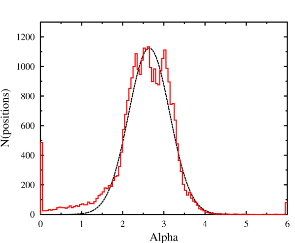
Figure 1: Histograms of the value of the extinction law parameter $\alpha$, calculated from the measured colour excess ratios using Eq. 3 (red). The best fit single gaussian to the distribution has $\mu=2.64$ with $\sigma=0.52$ is overlaid on the data (black).

Median colour excess is then obtained by subtracting a value for the average intrinsic colours for the stars. We used the average of the colours of G, K and M giant stars as taken from Cox (2000, and references therein) to obtain colour excesses for the Nuclear Bulge stars. We use G, K and M type stars as these are the most common stellar types in the Nuclear Bulge. We also set a threshold limit of 5 stars within the $10\arcsec$ sampling box as a minimum for the number of stars required for the scripts to calculate a specific extinction. If there are fewer than this number in the sample region, the value for that point for both the $10\arcsec$ and $20\arcsec$ sampling is set to the average value measured for the whole field.

The colour excess ratios for each grid point were then used to identify the value of the extinction law parameter $\alpha$ by comparison to tables of values generated using equation 3. We then used this value of $\alpha$ to calculate the value of $C$ at that position using equation 2, and then the absolute extinction in $J$, $H$ and $K_{\rm S}$-bands was calculated using equation 1.

5 The Extinction

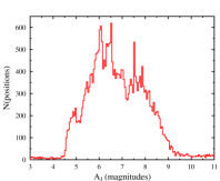
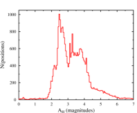
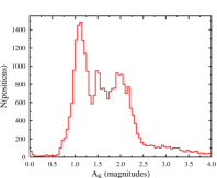
Figure 2: Histograms of the values of absolute extinction calculated for all grid points. Each histogram represents the absolute extinction of a specific wavelength; left is $A_{J}$, centre is $A_{H}$ and right is $A_{K_{\rm S}}$.

5.1 Measured Extinction Law

Figure 1 shows a histogram of the values of $\alpha$ measured for all the fields using the colour excess ratio method in Eq. 3 with a single gaussian fit to the distribution.

The distribution of $\alpha$ is well fit by a single gaussian with $\mu=2.64$ and $\sigma=0.52$. Errors in the intrinsic measured magnitudes of the stars are the largest source of error in the measurement of the colour excesses from which each value of $\alpha$ is obtained, but the large sample ($>30,000$ positions) results in a vanishingly small error in the mean and standard deviation as measured from the histograms. The binning for the histograms is 0.05 in values of $\alpha$; the error in the fit of the gaussian to the histogram is comparable to one histogram bin.

5.2 Measured Extinction

Using the value of $\alpha$ measured at each point in the fields, we calculated the absolute extinction from the colour excesses using equation 2 to obtain a value for $C$ and equation 1 to calculate the extinction for each wavelength. Figure 2 shows histograms of the values of absolute extinction for each wavelength, calculated at all grid points in the 26 VLT fields.

All three distributions of absolute extinction have common features. The values of extinction are generally confined to a single range of values, with almost no cells having values outside this range. Within this range, there is a small, low-extinction component, the main component of the extinction is then one large peak at an absolute extinction a little higher than the low extinction component. Beyond this initial peak there is a plateau extending to higher levels of extinction before a relatively sharp cut-off. At the cut-off there is then a smaller component that forms a tail extending to very high levels of extinction. That these features are common to all three wavelengths suggests that the different wavelengths are showing different representations of a common distribution of extincting material and not different materials acting at different wavelengths.

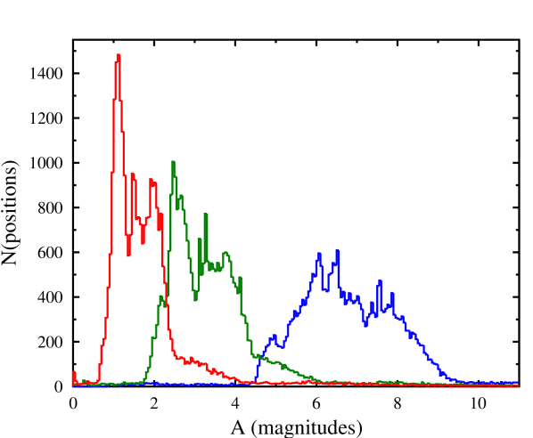
Figure 3: Histogram of the amount of extinction in magnitudes at each position, in bins of $0.05\,{\rm mag}$. The blue curve (right) is the $A_{J}$ distribution, green (middle) is the $A_{H}$ distribution and red (left) is the $A_{K_{\rm S}}$ distribution.

The majority of the $A_{J}$ extinction is in the range $4.5\leq A_{J}\leq 9$, consisting of three peaks. The low-extinction component of the distribution peaks at $A_{J}=4.8$, the main component of the distribution peaks around $A_{J}=6.1$ and the higher extinction plateau region is centred around $A_{J}=7.8$.

The $A_{H}$ extinction distribution is in the range $1.5\leq A_{H}\leq 6.5$ with a proportionally smaller low extinction component and larger high extinction component. The low extinction component peaks around $A_{H}=2.1$. The stronger, main peak is around $A_{H}=2.5$ and the higher extinction plateau region stretches over about 1.5 mag in $A_{H}$ centred around $A_{H}=3.5$. There is also an small, even higher extinction tail extending between $4.5\leq A_{H}\leq 6$.

The $A_{K_{\rm S}}$ extinction distribution follows approximately the same distribution as the $A_{J}$ and $A_{H}$ above, in the range $0.5\leq A_{K_{\rm S}}\leq 4.5$. For $A_{K_{\rm S}}$ the low extinction component is almost not present, and the higher extinction plateau is more pronounced. The main, largest component of the distribution is centred on $A_{K_{\rm S}}=1.1$, and the higher extinction plateau extends from $1.3\leq A_{K_{\rm S}}\leq 2.5$ with two apparent peaks at $A_{K_{\rm S}}=1.55$ and $A_{K_{\rm S}}=2.05$. The high extinction tail extends from $A_{K_{\rm S}}=2.5$ out to approximately $A_{K_{\rm S}}=4.5$.

Figure 3 shows the three extinction distributions plotted on the same graph. This shows the differing values of the extinction compared to each other, and the similarity of the shapes of the three distributions. The three distributions appear to be a single distribution that is stretched at shorter wavelengths ($A_{J}$ is broader and lower than $A_{K_{\rm S}}$ for example). Figure 4 shows the extinction maps of three example fields showing the degree of variation within each $2.5\arcmin\times 2.5\arcmin$ field. Each pixel in these images corresponds to one of the grid points separated by 5″ as outlined in Section 4, and the colour scale represents $0\leq A_{H}\leq 10$.

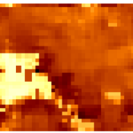
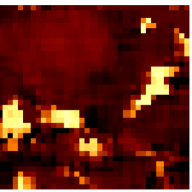
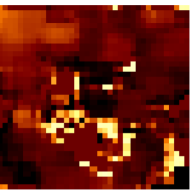
Figure 4: Maps of the measured extinction in three of the VLT fields in $A_{J}$. Each map fills the full extent of the $2.5\arcmin\times 2.5\arcmin$ VLT fields, and each pixel within each map represents the extinction in a region $5\arcsec\times 5\arcsec$. The colour scale represents variation in the absolute extinction in the range: $0\leq A_{J}\leq 10$.

5.3 Comparison with non-varying Extinction Law

In order to test the significance of the variation in the extinction law, we re-ran our extinction calculation twice, once allowing the value of the extinction law parameter $\alpha$ to vary from field to field but not within the field and a second time using the mean extinction law parameter for all of the fields, $\alpha=2.64$ (see Figure 1). To measure the effects, we compared how the value of absolute extinction calculated using equations 1 changes for the different colour excesses (for example: the difference between $A_{J}$ calculated from $\left<E(J\!-\!H)\right>$ and $\left<E(J\!-\!K_{\rm S})\right>$). We measured the difference using a $\chi_{\nu}^{2}$ test for each value of $A_{\lambda}$.

For the fully varying, V-NICE extinction calculation method that we are presenting in this paper, the $\chi_{\nu}^{2}$ test returned values in the range $1.34-2.37$, indicating that the variation between the measures is within one or two $\sigma$ of the distribution for almost all cases (Table 1). Allowing the extinction law to vary from one field to another, but not within the field, we find that the differences in the values of absolute extinction calculated from different colour excesses result in a $\chi_{\nu}^{2}$ test returning results of $10.78-15.35$. This illustrates that there is a statistically significant difference between the distributions of absolute extinction calculated for each wavelength from the two applicable colour excesses when keeping the extinction law constant across individual fields rather than allowing it to vary within a given field. In other words, if the value of $\alpha$ is held constant over the 2.5 arcmin² of any one VLT field, different values of the absolute extinction (i.e.: $A_{J}$) will be calculated depending upon which colour excess is used (i.e.: $\left<E(J\!-\!H)\right>$ or $\left<E(J\!-\!K_{\rm S})\right>$). This illustrates that it is important to allow for variation in the extinction law on as small a scale as is possible for any dataset to derive the most accurate measure of the extinction in a given field.

The final re-run of the extinction calculation used a single extinction law, fixed at the average value for all the fields ($\alpha=2.64\pm 0.52$) as measured in Figure 1, to convert colour excess to absolute extinction for all 26 of the VLT fields. This is similar to the method that has previously been used to calculate the extinction throughout the Galaxy where variations in extinction law have rarely been taken into account. In this case there were obvious differences in the calculated values of absolute extinction from the different colour excesses, revealed by the $\chi_{\nu}^{2}$ test which returned values of $19.85-55.05$.

5.4 Intrinsic effects of filters

We note that the value of the extinction law parameter $\alpha$ that we measure from our data is significantly different from the more generally accepted value $\alpha\sim 2$ (Rieke & Lebofsky, 1985; Cardelli et al., 1989; Mathis, 1990; Nishiyama et al., 2006, and others). Here we consider that the method that we use to calculate the extinction law parameter may be affecting the measured value. In equation 3, it is assumed that the filters in the telescope system used are infinitely thin, whereas in reality they admit light over a range of wavelengths with varying efficiency, the transmission profile. It is possible that in sampling a larger bandwidth of the stellar spectra than only at the central wavelengths as assumed in our methods; the filter transmission profiles are the cause of the difference of our measured values of $\alpha$ from previous studies.

To explore this, we simulated the effects of using both a narrow idealized filter, as assumed in our extinction calculation method, and the real transmission functions of the VLT-ISAAC filters as given on the ESO website. To simulate the narrow filters we used thin gaussians with peak transmission efficiency of 1 and width of $100\,{\rm\AA}$ centred on the quoted central wavelengths of the VLT-ISAAC filters. For the actual filter case, we could only apply the filter transmission functions as there is no comprehensive data available on the ESO website which takes into account the additional effects of the atmosphere, telescope and instrument optical path on light transmission in VLT-ISAAC. Experience suggests that these effects will be predominately attenuation of the light transmitted through the system and so the filter transmission function will have the largest effect on variation in the measured extinction. We used a sample of stellar spectra, G, K and M type giants from the Pickles (1998) libraries, and applied extinction to all spectra with a power-law wavelength dependence $A_{\lambda}\propto\lambda^{-\alpha}$. We used $\alpha=2$ for the extinction applied to the spectra as that is the most commonly used value for extinction in the near-infrared and it also allows us to compare the results to the values we measured with our V-NICE method. We then used the IRAF package synphot to pass the extincted standard star spectra through the two filter sets described above. We used the magnitudes output by the synphot package for the different filters to calculate colour excess for the spectral types, and from the colour excess calculated the extinction law parameter $\alpha$ using equation 3.

Table 1: Results of the tests of the effect of extinction law variation on calculated absolute extinction for three scenarios: one with a fully variable extinction law (top), one with an extinction law fixed for individual fields (middle) and one with a single extinction law for all fields (bottom). For each instance, the differences in the values of absolute extinction for a single wavelength calculated from the two applicable colour excesses are compared with a $\chi_{\nu}^{2}$ test. The results of these $\chi_{\nu}^{2}$ tests are presented against the colour excess error used in their calculation. It shows that the fully variable extinction law produces the most consistent calculation of absolute extinction from different colour excesses and that a fixed extinction law produces the worst.

Colour excess			Colour excess
error used	$\chi_{\nu}^{2}$		error used	$\chi_{\nu}^{2}$
Fully variable extinction law
$A_{J}\left<E(J\!-\!H)\right>$	2.3675		$A_{J}\left<E(J\!-\!K_{\rm S})\right>$	2.2644
$A_{H}\left<E(J\!-\!H)\right>$	1.3412		$A_{H}\left<E(H\!-\!K_{\rm S})\right>$	1.8251
$A_{K_{\rm S}}\left<E(J\!-\!K_{\rm S})\right>$	1.7369		$A_{K_{\rm S}}\left<E(H\!-\!K_{\rm S})\right>$	2.0890
Single extinction law for each field
$A_{J}\left<E(J\!-\!H)\right>$	12.0757		$A_{J}\left<E(J\!-\!K_{\rm S})\right>$	10.7796
$A_{H}\left<E(J\!-\!H)\right>$	12.7166		$A_{H}\left<E(H\!-\!K_{\rm S})\right>$	15.3468
$A_{K_{\rm S}}\left<E(J\!-\!K_{\rm S})\right>$	12.4007		$A_{K_{\rm S}}\left<E(H\!-\!K_{\rm S})\right>$	14.1556
Extinction law $\alpha=2.64$ applied to all fields
$A_{J}\left<E(J\!-\!H)\right>$	19.8532		$A_{J}\left<E(J\!-\!K_{\rm S})\right>$	21.2689
$A_{H}\left<E(J\!-\!H)\right>$	27.8859		$A_{H}\left<E(H\!-\!K_{\rm S})\right>$	55.0459
$A_{K_{\rm S}}\left<E(J\!-\!K_{\rm S})\right>$	34.4246		$A_{K_{\rm S}}\left<E(H\!-\!K_{\rm S})\right>$	39.5893

We found that the case of thin gaussians returns the true value of $\alpha=2.00\pm 0.05$, as expected. For the actual ISAAC filter transmission functions, the values of $\alpha$ measured for the different spectral types of the stars were in the range $1.75\leq\alpha\leq 1.85$. The variation in the measured extinction law corresponded to variation in the spectral types of the stars, earlier type stars resulted in a lower measured value of $\alpha$, and later types resulted in a higher measured value of $\alpha$ (within the range given above).

To average the effects of the different spectral types, and to recreate our actual method used to calculate extinction, namely sampling a variety of stars over a region of the sky, we selected 40–50 random spectral types, adding 5% noise to the measured magnitudes in all three bands, and calculated an average value for the extinction law for the combined colours of the stars. In 1000 repetitions, we measured a value of $\alpha=1.81\pm 0.11$ (the error being consistent with the random noise added to the simulated magnitudes).

6 Discussion

We have identified two significant sources of potential error in the calculation of the extinction in the near-infrared. First, there may be substantial significant variation in the extinction-wavelength power-law relationship parameter $\alpha$ (where $A_{\lambda}=C\times\lambda^{-\alpha}$) and in the absolute value of extinction $A_{\lambda}$, especially in heavily extinguished regions of the Galactic Bulge and Plane. Second, the measured values of $\alpha$ are influenced by the transmission profile of the instrument used to obtain the photometric data on which the extinction calculation is based.

6.1 Extinction calculation

We have applied our new V-NICE extinction calculation method which measures variation on small spatial scales in both the extinction law and the absolute extinction to fields distributed “randomly” throughout the Nuclear Bulge, avoiding known regions of star formation and structures such as the Arches and other clusters. As such, these fields offer a deeper, representative sample of the “general” Nuclear Bulge population than it has been possible to obtain from previous observations such as 2MASS. As we have demonstrated in Gosling et al. (2007), this method produces self-consistent measures of the extinction that can recover real photometric values for the extinction corrected stars. Until similar analysis can be undertaken on forthcoming near-infrared observations of the entire Nuclear Bulge, using data from the UKIDSS and VISTA surveys, this work represents the most generalised and representative study of the extinction of the overall Nuclear Bulge.

6.2 Extinction Law

In all fields we see variation in the measured extinction law on scales of $\sim\,5-10\arcsec$, which is also the scale of the granularity measured in Gosling et al. (2006). We measure a broad range of values of the extinction law parameter, in the range $0\leq\alpha\leq 4$. Fitting a gaussian to the extinction law parameter distribution, we find that the extinction law in the Nuclear Bulge can be described in the most general terms of $\alpha=2.64$ with a standard deviation of $0.52$ (see Figure 1).

We tested the variation in the extinction law parameter as measured with VLT-ISAAC, Table 1 shows the effect of the variation on the calculated absolute extinction when using different colour excesses. Only in the case of allowing full variation of the extinction law are the absolute extinction values calculated from different colour excesses the within $3\sigma$ limits. For the cases of a more general extinction law, a single value for each field and a single value for all fields, the differences introduced by the calculation of absolute extinction from different colour excesses are beyond what can be explained as statistical variations in the distributions (i.e.: differences greater than $3\sigma$). Additionally, in Gosling et al. (2007), we demonstrate that the use of a fully variant extinction law is the only way to obtain consistent photometry for stellar sources in our VLT fields and, by extension, throughout the Nuclear Bulge.

6.3 Absolute Extinction

We see considerable levels of variation in the measured absolute extinction on very small scales resulting in overall extinction ranges in the near-infrared of $4.5\leq A_{J}\leq 10$, $1.5\leq A_{H}\leq 6.5$ and $0.5\leq A_{K_{\rm S}}\leq 4.5$. The spread of the measured values of absolute extinction are similar for all three bands. Each has a small amount of very low levels of extinction, a large fraction centred on a single value, with a “plateau” of increasing values of extinction with a final, very small high extinction tail. That these distributions are similar, with the shorter wavelength distribution “stretched” indicates that all three near-infrared bands are measuring the same extincting material distribution. The variations we measure are on scales of $\sim\,5-10\arcsec$, the same scales at which we measured variation in the stellar distribution in Gosling et al. (2006). We interpret the distribution of different values of extinction as representing the distribution of these dense, obscuring clouds identified in our previous paper. The largest peak in all three distributions, at the lower end of the overall extinction distribution represents the “field” value away from these extincting structures, the higher extinction “plateaux” represent the extinction in the denser regions, the size scale of which we measured in Gosling et al. (2006). It is thus important to consider both the size of these structures, and their distribution when calculating the extinction in the Nuclear Bulge as applying a “field” value for the extinction could underestimate extinction by a factor of 2–3 if the target is close to or in one of these dense, complex regions.

The values of $A_{K_{\rm S}}$ are we measure similar to the values that have previously been measured, with the majority of the $A_{K_{\rm S}}$ distribution in the region of 1–3; however, due to the variable and generally greater value of the extinction law parameter $\alpha$, the values of $A_{J}$ and $A_{H}$ in this work are considerably higher than have previously been measured. Both our calculation of the extinction from different colour excesses (Section 5.3), and the extinction correction of stars in Gosling et al. (2007) for photometric identification indicate that this higher value of the extinction law parameter $\alpha$ and the small scale variations are the correct method to use in the Nuclear Bulge. The higher value of $\alpha$ means that previous works (Catchpole et al., 1990; Schultheis et al., 1999; Lombardi & Alves, 2001, and others) which quoted values of $A_{V}$ based on measures of extinction in the near-infrared will have significantly underestimated the values of $A_{V}$. As an example, the most commonly used conversion factor from near-infrared to visual is $A_{V}/A_{K_{\rm S}}=9$ (Rieke & Lebofsky, 1985); more recently Nishiyama et al. (2008) have reported that in areas of the outer Bulge, they measured a higher conversion factor of $A_{V}/A_{K_{\rm S}}\sim 16$. Using the conversion factors of Martin & Whittet (1990) and Rieke & Lebofsky (1985) to derive the mean relation between $A_{K_{\rm S}}$ and $A_{V}$, our work would suggest a conversion factor of $A_{V}/A_{K_{\rm S}}=28.7^{+17.2}_{-11.7}$ in the Nuclear Bulge for $\alpha=2.64\pm 0.52$, 3 times higher than the most commonly used value.

6.4 Measuring the Extinction

We recommend that wherever possible, i.e. if data from at least three infrared bands is available for a given location, a specific calculation of the extinction be carried out to obtain accurate stellar photometry in heavily extinguished regions of the sky such as the Nuclear Bulge. Due to the very small scale, real variation that we measure in the extinction law in this region, it is extremely important that as local a value as possible is measured. Using our V-NICE method allows for the very small spatial variations in the extinction law parameter $\alpha$ as well as the absolute extinction, producing the most accurate measure of the extinction at different wavelengths in the near-infrared.

6.5 Filter transmission effects

As seen in Section 5.4, the transmission function of the filter-set used in observations has an effect on the value of the extinction law parameter measured using our method. The results suggest that only for an idealized very thin filter profile will the “real” value of the extinction law be measured using this method. For the broader filter profiles of real instruments, the spectral slope of the star being observed will influence the value of the extinction law measured. The spatial variations in the extinction law that we observe are not affected by this property, only the exact numerical value measured for $\alpha$. The result of this is that the extinction law parameter $\alpha$ and the absolute extinction measured from a set of observations using a unique telescope-instrument setup can only be applied to data from other observations using the same telescope-instrument combination without the need to account for the filter transmission. If the extinction correction values measured from one dataset are applied to data from observations obtained using other telescope-instrument combinations, an error will be induced by the differing filter transmissions.

7 Conclusions - A new Extinction measure

We have studied the extinction in the near-infrared in a sample of representative regions of the Nuclear Bulge based on observations with VLT-ISAAC. We have found a high degree of spatial variability in both the extinction law parameter $\alpha$ as well as the absolute extinction in these regions. We have used a new method, a variable near-infrared colour excess, V-NICE, to measure these variations. Only when the value of the extinction law parameter $\alpha$ as well as the absolute extinction is allowed to vary can self-consistent values for the extinction at different wavelengths in the near-infrared be calculated.

For our observations, using VLT-ISAAC, the peak of the extinction law parameter $\alpha$’s distribution for the Nuclear Bulge is at a higher value than previously thought, described by a gaussian with $\mu=2.64$ and $\sigma=0.52$. We allowed the extinction law to vary when calculating the absolute extinction at different wavelengths from colour excesses and show that only when this variation is allowed can self-consistent levels of extinction be recovered. The variations of both the extinction law parameter $\alpha$ and the absolute extinction are seen on scales as small as $5\arcsec$. We measure extinction in the near-infrared of $4.5\leq A_{J}\leq 10$, $1.5\leq A_{H}\leq 6.5$ and $0.5\leq A_{K_{\rm S}}\leq 4.5$. The higher overall value of the extinction law parameter $\alpha$ results in a higher conversion factor between $A_{J}$, $A_{H}$ and $A_{K_{\rm S}}$. This suggests that previously derived levels of $A_{\lambda}$ in the Nuclear Bulge from near-infrared extinction measures may need to be reconsidered.

We have also found that the extinction law parameter $\alpha$ has a dependency on the transmission function of the instrument. We simulated the effects of the instrument filter transmission profiles on the measured value of the extinction law parameter $\alpha$ and showed that in the case of idealized narrow filters, our method recovers the true value of the extinction law, but for the real ISAAC filter transmission profiles, the result measured is $\sim\,10\%$ below the true value.

The effects of the small scale variation in the extinction law as well as the absolute extinction are the dominant source of errors when correcting for extinction in the Nuclear Bulge. Furthermore, we suggest that the potential for small-scale physical variations in the extinction should be considered when performing photometry in any significantly extinguished area of the Galactic Bulge or Plane. The method presented here is sufficient to obtain accurate stellar photometry for multi-colour data from any near-infrared telescope-instrument combination, and can be used to correct for extinction to allow identification of stellar types by comparison to photometric standards. The exact extinction values measured will be relative to the telescope-instrument combination. Unless the absolute value of extinction law is required, or the measured extinction will be used to correct the colours of stars from datasets from other combinations of telescope and instrument, the effects of the filter transmission effects discussed here need not be considered. However, if the measured extinction law value is used to reddening-correct data from different telescope-instrument combinations, the user should be aware of the errors that will be induced by the different filter transmission profiles.

Due to these two effects, we suggest that the use of a generic “universal” IR extinction law is not appropriate in many cases, especially when observing regions of the Galaxy known to suffer significant extinction. We recommend that whenever possible, a local extinction calculation should be undertaken as this provides the most accurate possible photometry for Bulge stars (Gosling et al., 2007). We suggest that the measure of granularity from Gosling et al. (2006) be used to determine the scale at which the extinction is variable and this be used to determine a limit to the area over which stars can be sampled in calculating the extinction. The methods we present here are an effective and accurate way of calculating the extinction for a dataset to correct the extinction towards sources in the Nuclear Bulge in the near-infrared.

Acknowledgements

The authors would like to thank the referee Prof. Edward Fitzpatrick for his extremely thorough reading of this manuscript and detailed points which have greatly improved this work. AJG would like to thank S.T.F.C. and Suomen Akatemia for grants funding his research. KMB thanks the Royal Society and the Leverhulme Trust for research support. This paper is based on observations made with the ESO VLT at Paranal under imaging programme ID 071.D-0377(A).

References

- Bandyopadhyay et al. (2005) Bandyopadhyay, R. M., et al. 2005, MNRAS, 364, 1195
- Bernstein et al. (2002) Bernstein, R. A., Freedman, W. L., & Madore, B. F. 2002, ApJ, 571, 107
- Blum et al. (1996) Blum, R. D., Sellgren, K., & Depoy, D. L. 1996, ApJ, 470, 864
- Cardelli et al. (1989) Cardelli, J. A., Clayton, G. C., & Mathis, J. S. 1989, ApJ, 345, 245
- Catchpole et al. (1990) Catchpole, R. M., Whitelock, P. A., & Glass, I. S. 1990, MNRAS, 247, 479
- Cox (2000) Cox, A. N. 2000, Allen’s astrophysical quantities, 4th ed. Publisher: New York: AIP Press; Springer, 2000. Editedy by Arthur N. Cox. ISBN: 0387987460,
- Davis et al. (1986) Davis, D. S., Larson, H. P., & Hofmann, R. 1986, ApJ, 304, 481
- Draine (2003) Draine, B. T. 2003, ARA&A, 41, 241
- Dutra et al. (2002) Dutra, C. M., Santiago, B. X., & Bica, E. 2002, A&A, 381, 219
- Dutra et al. (2003) Dutra, C. M., Santiago, B. X., Bica, E. L. D., & Barbuy, B. 2003, MNRAS, 338, 253
- Froebrich & del Burgo (2006) Froebrich, D., & del Burgo, C. 2006, MNRAS, 369, 1901
- Froebrich et al. (2007) Froebrich, D., Murphy, G. C., Smith, M. D., & Walsh, J. 2007, ArXiv e-prints, 704, arXiv:0704.2993
- Fitzpatrick (2004) Fitzpatrick, E. L. 2004, ASP Conf. Ser. 309: Astrophysics of Dust, 309, 33
- Fitzpatrik & Massa (2007) Fitzpatrick, E. L., & Massa, D. 2007, ArXiv e-prints, 705, arXiv:0705.0154
- Glass (1999) Glass, I. S. 1999, Handbook of infrared astronomy, (CUP)
- Gordon et al. (2003) Gordon, K. D., Clayton, G. C., Misselt, K. A., Landolt, A. U., & Wolff, M. J. 2003, ApJ, 594, 279
- Gosling et al. (2006) Gosling, A. J., Blundell, K. M., & Bandyopadhyay, R. 2006, ApJL, 640, L171
- Gosling et al. (2007) Gosling, A. J., Bandyopadhyay, R. M., Miller-Jones, J. C. A., & Farrell, S. A. 2007, MNRAS, 380, 1511
- Jones & Hyland (1980) Jones, T. J., & Hyland, A. R. 1980, MNRAS, 192, 359
- Kenyon et al. (1998) Kenyon, S. J., Lada, E. A., & Barsony, M. 1998, AJ, 115, 252
- Lombardi & Alves (2001) Lombardi, M., & Alves, J. 2001, A&A, 377, 1023
- Martin & Whittet (1990) Martin, P. G., & Whittet, D. C. B. 1990, ApJ, 357, 113
- Mathis (1990) Mathis, J. S. 1990, ARA&A, 28, 37
- Messineo et al. (2005) Messineo, M., Habing, H. J., Menten, K. M., Omont, A., Sjouwerman, L. O., & Bertoldi, F. 2005, A&A, 435, 575
- Mezger et al. (1996) Mezger, P. G., Duschl, W. J., & Zylka, R. 1996, A&AR, 7, 289
- Nishiyama et al. (2006) Nishiyama, S., et al. 2006, ApJ, 638, 839
- Nishiyama et al. (2008) Nishiyama, S., Nagata, T., Tamura, M., Kandori, R., Hatano, H., Sato, S., & Sugitani, K. 2008, ArXiv e-prints, 802, arXiv:0802.3559
- Pickles (1998) Pickles, A. J. 1998, PASP, 110, 863
- Rieke & Lebofsky (1985) Rieke, G. H., & Lebofsky, M. J. 1985, ApJ, 288, 618
- Rodríguez-Fernández & Martín-Pintado (2005) Rodríguez-Fernández, N. J., & Martín-Pintado, J. 2005, A&A, 429, 923
- Savage & Mathis (1979) Savage, B. D., & Mathis, J. S. 1979, ARA&A, 17, 73
- Schultheis et al. (1999) Schultheis, M., et al. 1999, A&A, 349, L69
- Udalski (2003) Udalski, A. 2003, ApJ, 590, 284
- Whittet et al. (1993) Whittet, D. C. B., Martin, P. G., Fitzpatrick, E. L., & Massa, D. 1993, ApJ, 408, 573