A mathematical proof of the existence of
trends in financial time series

Abstract

We are settling a longstanding quarrel in quantitative finance by proving the existence of trends in financial time series thanks to a theorem due to P. Cartier and Y. Perrin, which is expressed in the language of nonstandard analysis (Integration over finite sets, F. & M. Diener (Eds): Nonstandard Analysis in Practice, Springer, 1995, pp. 195–204). Those trends, which might coexist with some altered random walk paradigm and efficient market hypothesis, seem nevertheless difficult to reconcile with the celebrated Black-Scholes model. They are estimated via recent techniques stemming from control and signal theory. Several quite convincing computer simulations on the forecast of various financial quantities are depicted. We conclude by discussing the rôle of probability theory.

Keywords:

Financial time series, mathematical finance, technical analysis, trends, random walks, efficient markets, forecasting, volatility, heteroscedasticity, quickly fluctuating functions, low-pass filters, nonstandard analysis, operational calculus.

1 Introduction

Our aim is to settle a severe and longstanding quarrel between

1. the paradigm of random walks and the related efficient market hypothesis [16] which are the bread and butter of modern financial mathematics,

2. the existence of trends which is the key assumption in technical analysis.

There are many publications questioning the existence either of trends (see, e.g., [16, 37, 48]), of random walks (see, e.g., [32, 56]), or of the market efficiency (see, e.g., [24, 52, 56]).

A theorem due to Cartier and Perrin [10], which is stated in the language of nonstandard analysis, yields the existence of trends for time series under a very weak integrability assumption. The time series $f(t)$ may then be decomposed as a sum

$$f(t)=f_{\tiny{\rm trend}}(t)+f_{\tiny{\rm fluctuation}}(t)$$ (1)

where

• $f_{\tiny{\rm trend}}(t)$ is the trend,

• $f_{\tiny{\rm fluctuation}}(t)$ is a “quickly fluctuating” function around $0$.

The very “nature” of those quick fluctuations is left unknown and nothing prevents us from assuming that $f_{\tiny{\rm fluctuation}}(t)$ is random and/or fractal. It implies the following conclusion which seems to be rather unexpected in the existing literature:

The two above alternatives are not necessarily contradictory and may coexist for a given time series.

We nevertheless show that it might be difficult to reconcile with our setting the celebrated Black-Scholes model [9], which is in the heart of the approach to quantitative finance via stochastic differential equations (see, e.g., [53] and the references therein).

Consider, as usual in signal, control, and in other engineering sciences, $f_{\tiny{\rm fluctuation}}(t)$ in Eq. (1) as an additive corrupting noise. We attenuate it, i.e., we obtain an estimation of $f_{\tiny{\rm trend}}(t)$ by an appropriate filtering. These filters

• are deduced from our approach to noises via nonstandard analysis [17], which

  • is strongly connected to this work,

  • led recently to many successful results in signal and in control (see the references in [18]),

• yields excellent numerical differentiation [40], which is here again of utmost importance (see also [19, 21] and the references therein for applications in control and signal).

A mathematical definition of trends and effective means for estimating them, which were missing until now, bear important consequences on the study of financial time series, which were sketched in [20]:

• The forecast of the trend is possible on a “short” time interval under the assumption of a lack of abrupt changes, whereas the forecast of the “accurate” numerical value at a given time instant is meaningless and should be abandoned.

• The fluctuations of the numerical values around the trend lead to new ways for computing standard deviation, skewness, and kurtosis, which may be forecasted to some extent.

• The position of the numerical values above or under the trend may be forecasted to some extent.

The quite convincing computer simulations reported in Sect. 4 show that we are

• offering for technical analysis a sound theoretical basis (see also [15, 33]),

• on the verge of producing on-line indicators for short time trading, which are easily implementable on computers.

Remark 1.

We utilize as in [20] the differences between the actual prices and the trend for computing quantities like standard deviation, skewness, kurtosis. This is a major departure from today’s literature where those quantities are obtained via returns and/or logarithmic returns, and where trends do not play any rôle. It might yield a new understanding of “volatility”, and therefore a new model-free risk management.

Our paper is organized as follows. Sect. 2 proves the existence of trends, which seem to contradict the Black-Scholes model. Sect. 3 sketches the trend estimation by mimicking [21]. Several computer simulations are depicted in Sect. 4. Sect. 5 concludes by examining probability theory in finance.

2 Existence of trends

2.1 Nonstandard analysis

Nonstandard analysis was discovered in the early 60’s by Robinson [51]. It vindicates Leibniz’s ideas on “infinitely small” and “infinitely large” numbers and is based on deep concepts and results from mathematical logic. There exists another presentation due to Nelson [46], where the logical background is less demanding (see, e.g., [13, 14, 50] for excellent introductions). Nelson’s approach [47] of probability along those lines had a lasting influence. As demonstrated by Harthong [26], Lobry [34], and several other authors, nonstandard analysis is also a marvelous tool for clarifying in a most intuitive way questions stemming from some applied sides of science. This work is another step in that direction, like [17, 18].

2.2 Sketch of the Cartier-Perrin theorem

2.2.1 Discrete Lebesgue measure and $S$-integrability

Let $\mathfrak{I}$ be an interval of $\mathbb{R}$, with extremities $a$ and $b$. A sequence $\mathfrak{T}=\{0=t_{0}<t_{1}<\dots<t_{\nu}=1\}$ is called an approximation of $\mathfrak{I}$, or a near interval, if $t_{i+1}-t_{i}$ is infinitesimal for $0\leq i<\nu$. The Lebesgue measure on $\mathfrak{T}$ is the function $m$ defined on $\mathfrak{T}\backslash\{b\}$ by $m(t_{i})=t_{i+1}-t_{i}$. The measure of any interval $[c,d[\subset\mathfrak{I}$, $c\leq d$, is its length $d-c$. The integral over $[c,d[$ of the function $f:\mathfrak{I}\rightarrow\mathbb{R}$ is the sum

$$\int_{[c,d[}fdm=\sum_{t\in[c,d[}f(t)m(t)$$

The function $f:\mathfrak{T}\rightarrow\mathbb{R}$ is said to be $S$-integrable if, and only if, for any interval $[c,d[$ the integral $\int_{[c,d[}|f|dm$ is limited and, if $d-c$ is infinitesimal, also infinitesimal.

2.2.2 Continuity and Lebesgue integrability

The function $f$ is said to be $S$-continuous at $t_{\iota}\in\mathfrak{T}$ if, and only if, $f(t_{\iota})\simeq f(\tau)$ when $t_{\iota}\simeq\tau$. The function $f$ is said to be almost continuous if, and only if, it is $S$-continuous on $\mathfrak{T}\setminus R$, where $R$ is a rare subset. We say that $f$ is Lebesgue integrable if, and only if, it is $S$-integrable and almost continuous.

2.2.3 Quickly fluctuating functions

A function $h:\mathfrak{T}\rightarrow\mathbb{R}$ is said to be quickly fluctuating, or oscillating, if, and only if, it is $S$-integrable and $\int_{A}hdm$ is infinitesimal for any quadrable subset.

Theorem 2.1.

Let $f:\mathfrak{T}\rightarrow\mathbb{R}$ be an $S$-integrable function. Then the decomposition (1) holds where

• $f_{\tiny{\rm trend}}(t)$ is Lebesgue integrable,

• $f_{\tiny{\rm fluctuation}}(t)$ is quickly fluctuating.

The decomposition (1) is unique up to an infinitesimal.

$f_{\tiny{\rm trend}}(t)$ and $f_{\tiny{\rm fluctuation}}(t)$ are respectively called the trend and the quick fluctuations of $f$. They are unique up to an infinitesimal.

2.3 The Black-Scholes model

The well known Black-Scholes model [9], which describes the price evolution of some stock options, is the Itô stochastic differential equation

$$dS_{t}=\mu S_{t}+\sigma S_{t}dW_{t}$$ (2)

where

• $W_{t}$ is a standard Wiener process,

• the volatility $\sigma$ and the drift, or trend, $\mu$ are assumed to be constant.

This model and its numerous generalizations are playing a major rôle in financial mathematics since more than thirty years although Eq. (2) is often severely criticized (see, e.g., [39, 55] and the references therein).

The solution of Eq. (2) is the geometric Brownian motion which reads

$$S_{t}=S_{0}\exp\left((\mu-\frac{\sigma^{2}}{2})t+\sigma W_{t}\right)$$

where $S_{0}$ is the initial condition. It seems most natural to consider the mean $S_{0}e^{\mu t}$ of $S_{t}$ as the trend of $S_{t}$. This choice unfortunately does not agree with the following fact: $F_{t}=S_{t}-S_{0}e^{\mu t}$ is almost surely not a quickly fluctuating function around $0$, i.e., the probability that $|\int_{0}^{T}F_{\tau}d\tau|>\epsilon>0$, $T>0$, is not “small”, when

• $\epsilon$ is “small”,

• $T$ is neither “small” nor “large”.

Remark 2.

A rigorous treatment, which would agree with nonstandard analysis (see, e.g., [3, 7]), may be deduced from some infinitesimal time-sampling of Eq. (2), like the Cox-Ross-Rubinstein one [12].

Remark 3.

Many assumptions concerning Eq. (2) are relaxed in the literature (see, e.g., [53] and the references therein):

• $\mu$ and $\sigma$ are no more constant and may be time-dependent and/or $S_{t}$-dependent.

• Eq. (2) is no more driven by a Wiener process but by more complex random processes which might exhibit jumps in order to deal with “extreme events”.

The conclusion reached before should not be modified, i.e., the price is not oscillating around its trend.

2.4 Returns

Assume that the function $f:\mathfrak{I}\rightarrow\mathbb{R}$ gives the prices of some financial asset. It implies that the values of $f$ are positive. What is usually studied in quantitative finance are the return

$$r(t_{i})=\frac{f(t_{i})-f(t_{i-1})}{f(t_{i-1})}$$ (3)

and the logarithmic return, or log-return,

$$\mathbf{r}(t_{i})=\log(f(t_{i}))-\log(f(t_{i-1}))=\log\left(\frac{f(t_{i})}{f(t_{i-1})}\right)=\log\left(1+r(t_{i})\right)$$ (4)

which are defined for $t_{i}\in\mathfrak{T}\backslash\{a\}$. There is a huge literature investigating the statistical properties of the two above returns, i.e., of the time series (3) and (4).

Remark 4.

Returns and log-returns are less interesting for us since the trends of the original time series are difficult to detect on them. Note moreover that the returns and log-returns which are associated to the Black-Scholes equation (2) via some infinitesimal time-sampling [3, 7] are not $S$-integrable: Theorem 2.1 does not hold for the corresponding time series (3) and (4).

Assume that the trend $f_{\tiny{\mbox{\rm trend}}}:\mathfrak{I}\rightarrow\mathbb{R}$ is $S$-continuous at $t=t_{i}$. Then Eq. (1) yields

$$f(t_{i})-f(t_{i-1})\simeq f_{\tiny{\mbox{\rm fluctuation}}}(t_{i})-f_{\tiny{\mbox{\rm fluctuation}}}(t_{i-1})$$

Thus

$$r(t_{i})\simeq\frac{f_{\tiny{\mbox{\rm fluctuation}}}(t_{i})-f_{\tiny{\mbox{\rm fluctuation}}}(t_{i-1})}{f(t_{i-1})}$$

It yields the following crucial conclusion:
 
The existence of trends does not preclude, but does not imply either, the possibility of a fractal and/or random behavior for the returns (3) and (4) where the fast oscillating function $f_{\tiny{\mbox{\rm fluctuation}}}(t)$ would be fractal and/or random.

3 Trend estimation

Consider the real-valued polynomial function $x_{N}(t)=\sum_{\nu=0}^{N}x^{(\nu)}(0)\frac{t^{\nu}}{\nu!}\in\mathbb{R}[t]$, $t\geq 0$, of degree $N$. Rewrite it in the well known notations of operational calculus (see, e.g., [57]):

$$X_{N}(s)=\sum_{\nu=0}^{N}\frac{x^{(\nu)}(0)}{s^{\nu+1}}$$

Introduce $\frac{d}{ds}$, which is sometimes called the algebraic derivative [42, 43], and which corresponds in the time domain to the multiplication by $-t$. Multiply both sides by $\frac{d^{\alpha}}{ds^{\alpha}}s^{N+1}$, $\alpha=0,1,\dots,N$. The quantities $x^{(\nu)}(0)$, $\nu=0,1,\dots,N$, which are given by the triangular system of linear equations, are said to be linearly identifiable (see, e.g., [18]):

$$\frac{d^{\alpha}s^{N+1}X_{N}}{ds^{\alpha}}=\frac{d^{\alpha}}{ds^{\alpha}}\left(\sum_{\nu=0}^{N}x^{(\nu)}(0)s^{N-\nu}\right)$$ (5)

The time derivatives, i.e., $s^{\mu}\frac{d^{\iota}X_{N}}{ds^{\iota}}$, $\mu=1,\dots,N$, $0\leq\iota\leq N$, are removed by multiplying both sides of Eq. (5) by $s^{-\bar{N}}$, $\bar{N}>N$, which are expressed in the time domain by iterated time integrals.

Consider now a real-valued analytic time function defined by the convergent power series $x(t)=\sum_{\nu=0}^{\infty}x^{(\nu)}(0)\frac{t^{\nu}}{\nu!}$, $0\leq t<\rho$. Approximating $x(t)$ by its truncated Taylor expansion $x_{N}(t)=\sum_{\nu=0}^{N}x^{(\nu)}(0)\frac{t^{\nu}}{\nu!}$ yields as above derivatives estimates.

Remark 5.

The iterated time integrals are low-pass filters which attenuate the noises when viewed as in [17] as quickly fluctuating phenomena. See [40] for fundamental computational developments, which give as a byproduct most efficient estimations.

Remark 6.

See [22] for other studies on filters and estimation in economics and finance.

Remark 7.

See [56] for another viewpoint on a model-based trend estimation.

4 Some illustrative computer simulations

Consider the Arcelor-Mittal daily stock prices from 7 July 1997 until 27 October 2008.

4.1 1 day forecast

Figure 1: 1 day forecast – Prices (red –), filtered signal (blue –), forecasted signal (black - -)

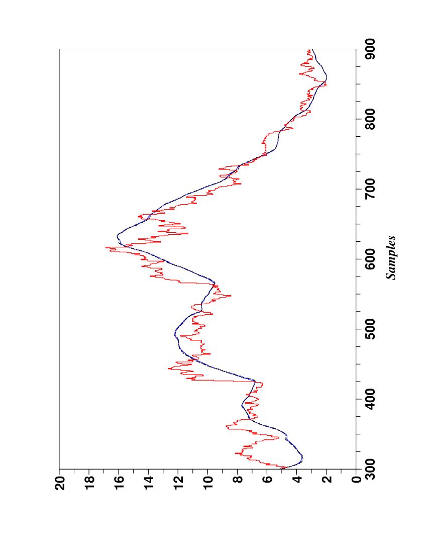
Figure 2: 1 day forecast – Zoom of figure 1

Figures 1 and 2 present

• the estimation of the trend thanks to the methods of Sect. 3, with $N=2$;

• a $1$ day forecast of the trend by employing a $2^{nd}$-order Taylor expansion. It necessitates the estimation of the first two trend derivatives which is also achieved via the methods of Sect. 3.

We now look at some properties of the quick fluctuations $f_{\tiny{\rm fluctuation}}(t)$ around the trend $f_{\tiny{\rm trend}}(t)$ of the price $f(t)$ (see Eq. (1)) by computing moving averages which correspond to various moments

$$MA_{k,M}(t)=\frac{\sum_{\tau=0}^{M}(f_{\tiny{\rm fluctuation}}(\tau-M)-\bar{f}_{\tiny{\rm fluctuation}})^{k}}{M+1}$$

where

• $k\geq 2$,

• $\bar{f}_{\tiny{\rm fluctuation}}$ is the mean of $f_{\tiny{\rm fluctuation}}$ over the $M+1$ samples,

• $M=100$ samples.

The standard deviation and its $1$ day forecast are displayed in Figure 3. Its heteroscedasticity is obvious.

The kurtosis $\frac{MA_{4,100}(t)}{MA_{2,100}(t)^{2}}$, the skewness $\frac{MA_{3,100}(t)}{MA_{2,100}(t)^{3/2}}$, and their $1$ day forecasts are respectively depicted in Figures 4 and 5. They show quite clearly that the prices do not exhibit Gaussian properties especially when they are close to some abrupt change.

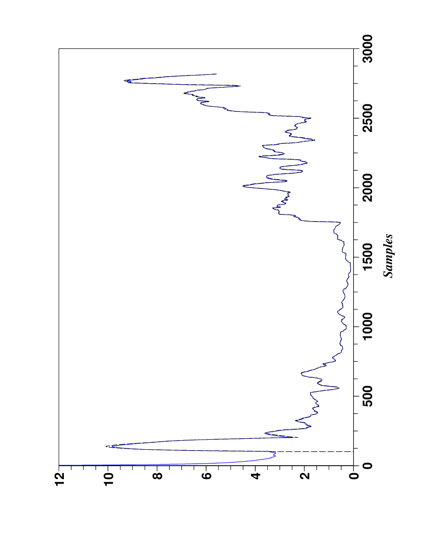
Figure 3: $1$ day forecast – Standard deviation w.r.t. trend (blue –), predicted standard deviation (black - -)

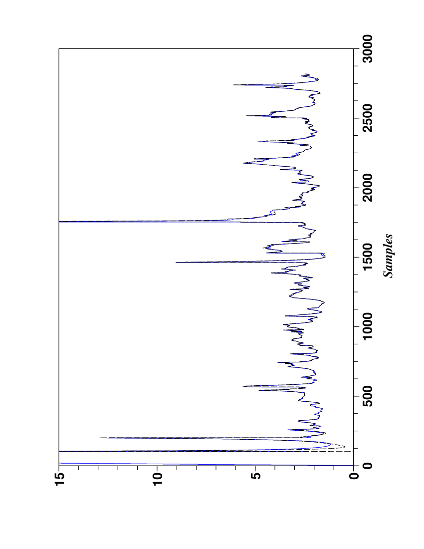
Figure 4: $1$ day forecast – Kurtosis w.r.t. trend (blue –), predicted kurtosis (black - -)

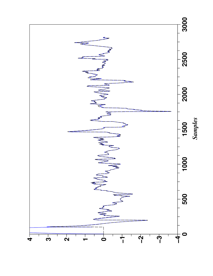
Figure 5: $1$ day forecast – Skewness w.r.t. trend (blue –), predicted skewness (black - -)

4.2 5 days forecast

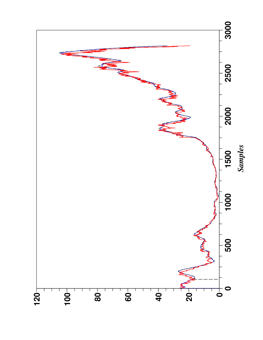
Figure 6: $5$ days forecast – Prices (red –), filtered signal (blue –), forecasted signal (black - -)

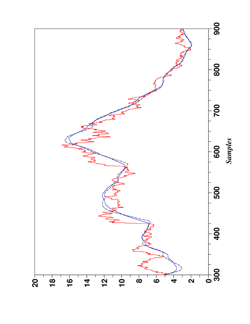
Figure 7: $5$ days forecast – Zoom of figure 6

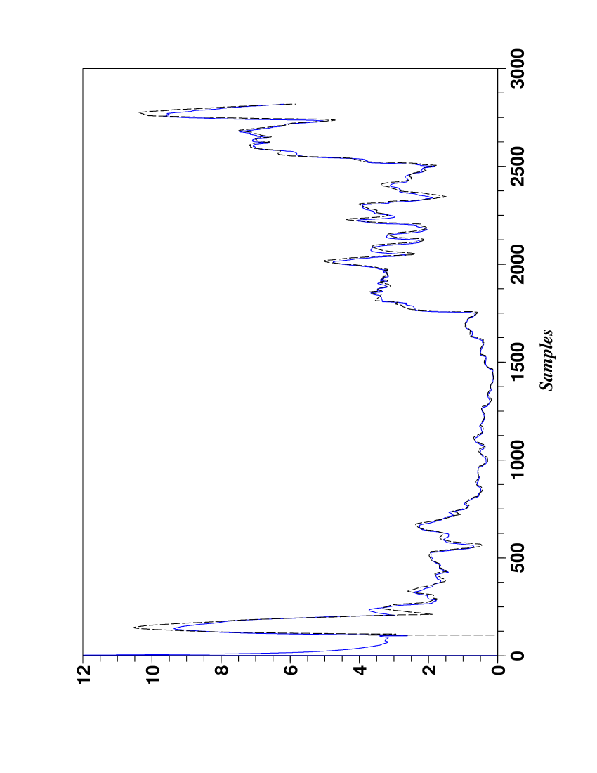
Figure 8: $5$ days forecast – Standard deviation w.r.t. trend (blue –), predicted standard deviation (black - -)

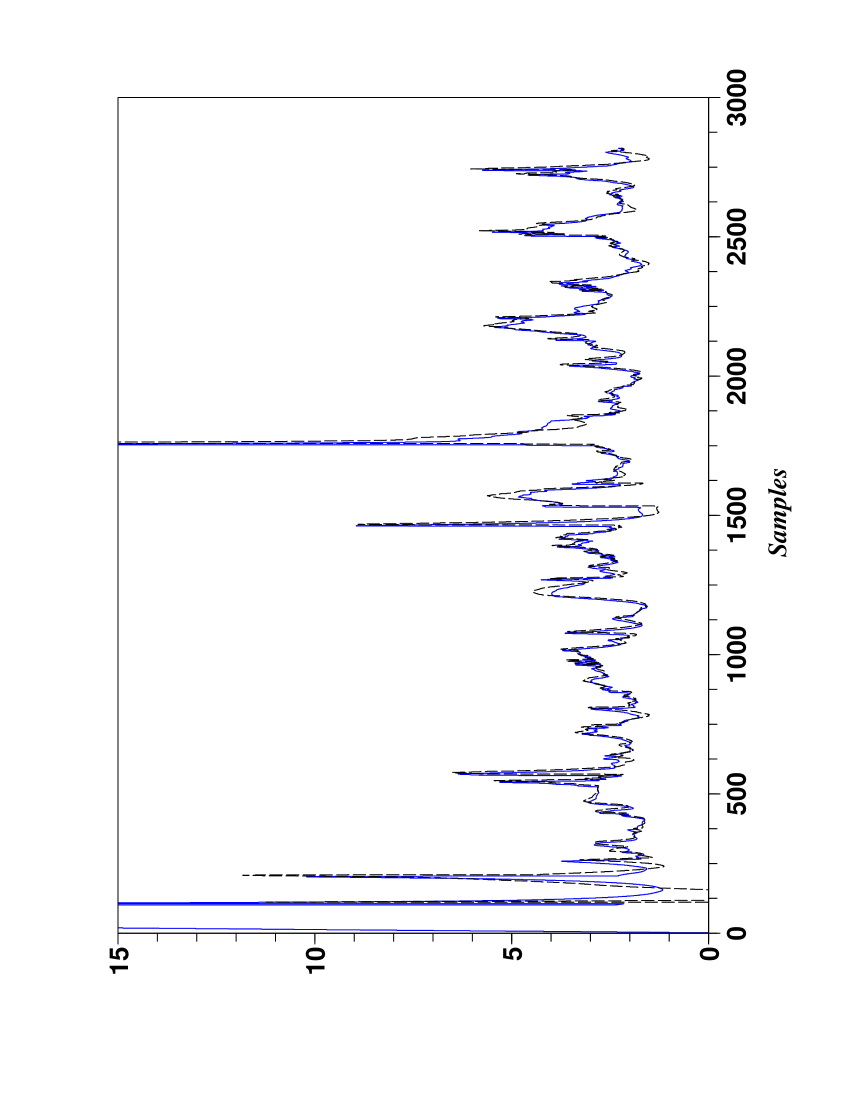
Figure 9: $5$ days forecast – Kurtosis w.r.t. trend (blue –), predicted kurtosis (black - -)

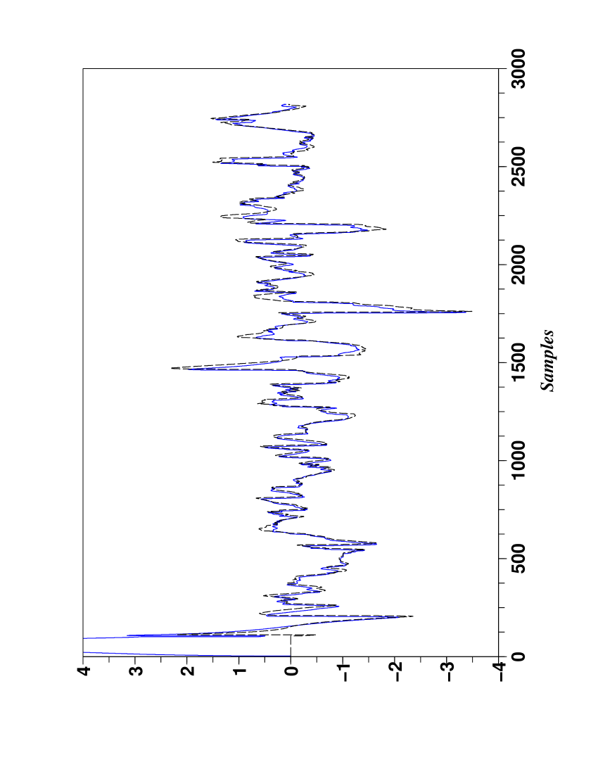
(a) Skewness of error trend (blue –), predicted skewness of error trend (black - -) (5 day ahead)

Figure 10: $5$ days forecast – Skewness w.r.t. trend (blue –), predicted skewness (black - -)

A slight degradation with a $5$ days forecast is visible on the Figures 6 to 10.

4.3 Above or under the trend?

Figure 11: $1$ day forecast – Prices (red –), predicted trend (blue - -), predicted confidence interval ($95\%$) (black –), price’s forecast higher than the predicted trend (green $\bigtriangleup$) , price’s forecast lower than the predicted trend (blue $\bigtriangledown$)

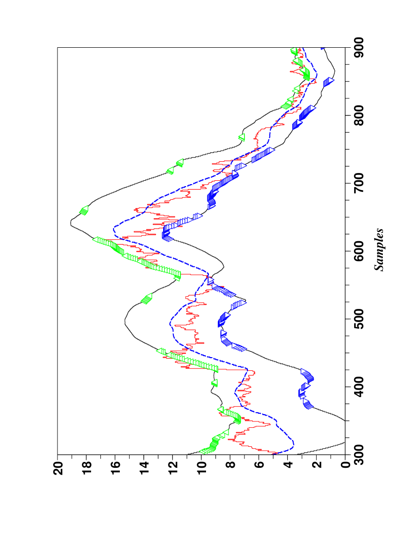
Figure 12: $1$ day forecast – Zoom of figure 11

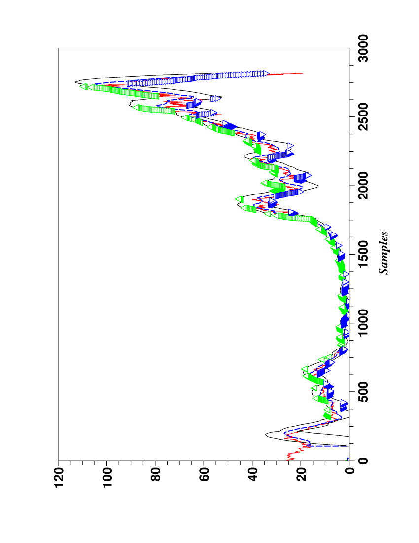
Figure 13: $5$ days forecast – Prices (red –), predicted trend (blue - -), predicted confidence interval ($95\%$) (black –), price’s forecast higher than the predicted trend (green $\bigtriangleup$) , value is forecasted as lower than predicted trend (blue $\bigtriangledown$)

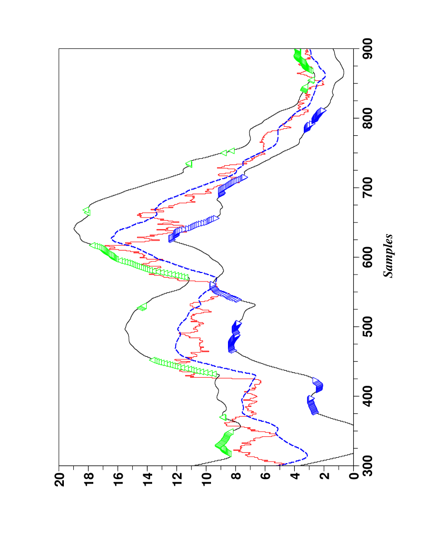
Figure 14: $5$ days forecast – Zoom of figure 13

Estimating the first two derivatives yields a forecast of the price position above or under the trend. The results reported in Figures 11-12 show for $1$ day (resp. $5$ days) ahead $75.69\%$ (resp. $68.55\%$) for an exact prediction, $3.54\%$ (resp. $3.69\%$) without any decision, $20.77\%$ (resp. $27.76\%$) for a wrong prediction.

5 Conclusion: probability in quantitative finance

The following question may arise at the end of this preliminary study on trends in financial time series:
 
Is it possible to improve the forecasts given here and in [20] by taking advantage of a precise probability law for the fluctuations around the trend?
 
Although Mandelbrot [38] has shown in a most convincing way more than forty years ago that the Gaussian character of the price variations should be at least questioned, it does not seem that the numerous investigations which have been carried on since then for finding other probability laws with jumps and/or with “fat tails” have been able to produce clear-cut results, i.e., results which are exploitable in practice (see, e.g., the enlightening discussions in [29, 39, 54] and the references therein). This shortcoming may be due to an “ontological mistake” on uncertainty:
 
Let us base our argument on new advances in model-free control [19]. Engineers know that obtaining the differential equations governing a concrete plant is always a most challenging task: it is quite difficult to incorporate in those equations frictions, heating effects, ageing, etc, which might have a huge influence on the plant’s behavior. The tools proposed in [19] for bypassing those equations got already in spite of their youth a few impressive industrial applications. This is an important gap between engineering’s practice and theoretical physics where the basic principles lead to equations describing “stylized” facts. The probability laws stemming from statistical and quantum physics can only be written down for “idealized” situations. Is it not therefore quite naïve to wish to exhibit well defined probability laws in quantitative finance, in economics and management, and in other social and psychological sciences, where the environmental world is much more involved than in any physical system? In other words a mathematical theory of uncertain sequences of events should not necessarily be confused with probability theory. To ask if the uncertainty of a “complex” system is of probabilistic nature is an undecidable metaphysical question which cannot be properly answered via experimental means. It should therefore be ignored.

Remark 8.

One should not misunderstand the authors. They fully recognize the mathematical beauty of probability theory and its numerous and exciting connections with physics. The authors are only expressing doubts about any modeling at large in quantitative finance, with or without probabilities.

The Cartier-Perrin theorem [10] which is decomposing a time series as a sum of a trend and a quickly fluctuating function might be

• a possible alternative to the probabilistic viewpoint,

• a useful tool for analyzing

  • different time scales,

  • complex behaviors, including abrupt changes, i.e., “rare” extreme events like financial crashes or booms, without having recourse to a model via differential or difference equations.

We hope to be able to show in a near future what are the benefits not only in quantitative finance but also for a new approach to time series in general (see [20] for a first draft).

References

- [1]
- [2] Aït-Sahalia Y., Lo A.W. Nonparametric risk management and implied risk aversion. J. Econometrics, 9, (2000) 9–51.
- [3] Albeverio S., Fenstad J.E., Hoegh-Krøhn R., Lindstrøm T. Nonstandard Methods in Stochastic Analysis and Mathematical Physics. Academic Press, 1986.
- [4] Bachelier L. Théorie de la spéculation. Ann. Sci. École Normale Sup. Sér. 3, 17, (1900) 21–86.
- [5] Béchu T., Bertrand E., Nebenzahl J. L’analyse technique (6e éd.). Economica, 2008.
- [6] Benoît E. Diffusions discrètes et mécanique stochastique. Prépubli. Lab. Math. J. Dieudonné, Université de Nice, 1989.
- [7] Benoît E. Random walks and stochastic differential equations. F. & M. Diener (Eds): Nonstandard Analysis in Practice. Springer, 1995, pp. 71–90.
- [8] Bernstein P.L. Capital Ideas: The Improbable Origins of Modern Wall Street. Free Press, 1992.
- [9] Black F., Scholes M. The pricing of options and corporate liabilities. J. Polit. Econ., 81, (1973) 637–654.
- [10] Cartier P., Perrin Y. Integration over finite sets. F. & M. Diener (Eds): Nonstandard Analysis in Practice. Springer, 1995, pp. 195–204.
- [11] Cootner P.H. The Random Characters of Stock Market Prices. MIT Press, 1964.
- [12] Cox J., Ross S., Rubinstein M. Option pricing: a simplified approach. J. Financial Econ., 7, (1979) 229–263.
- [13] Diener F., Diener M. Tutorial. F. & M. Diener (Eds): Nonstandard Analysis in Practice. Springer, 1995, pp. 1–21.
- [14] Diener F., Reeb G., Analyse non standard. Hermann, 1989.
- [15] Dacorogna M.M., Gençay R., Müller U., Olsen R.B., Pictet O.V. An Introduction to High Frequency Finance. Academic Press, 2001.
- [16] Fama E.F. Foundations of Finance: Portfolio Decisions and Securities Prices. Basic Books, 1976.
- [17] Fliess M. Analyse non standard du bruit. C.R. Acad. Sci. Paris Ser. I, 342, (2006) 797–802.
- [18] Fliess M. Critique du rapport signal à bruit en communications numériques. ARIMA, 9, (2008) 419–429. Available at http://hal.inria.fr/inria-00311719/en/.
- [19] Fliess M., Join C. Commande sans modèle et commande à modèle restreint, e-STA, 5, (2008) n∘ 4. Available at http://hal.inria.fr/inria-00288107/en/.
- [20] Fliess M., Join C. Time series technical analysis via new fast estimation methods: a preliminary study in mathematical finance. Proc. 23rd IAR Workshop Advanced Control Diagnosis (IAR-ACD08), Coventry, 2008. Available at http://hal.inria.fr/inria-00338099/en/.
- [21] Fliess M., Join C., Sira-Ramírez H. Non-linear estimation is easy, Int. J. Modelling Identification Control, 4, (2008) 12–27. Available at http://hal.inria.fr/inria-00158855/en/.
- [22] Gençay R., Selçuk F., Whitcher B. An Introduction to Wavelets and Other Filtering Methods in Finance and Economics. Academic Press, 2002.
- [23] Gouriéroux C., Monfort A. Séries temporelles et modèles dynamiques (2e éd.). Economica, 1995. English translation: Time Series and Dynamic Models. Cambridge University Press, 1996.
- [24] Grossman S., Stiglitz J. On the impossibility of informationally efficient markets. Amer. Economic Rev., 70, (1980) 393–405.
- [25] Hamilton J.D. Time Series Analysis. Princeton University Press, 1994.
- [26] Harthong J. Le moiré. Adv. Appl. Math., 2, (1981) 21–75.
- [27] Harthong J. La méthode de la moyennisation. M. Diener & C. Lobry (Eds): Analyse non standard et représentation du réel. OPU & CNRS, 1985, pp. 301–308.
- [28] Harthong J. Comment j’ai connu et compris Georges Reeb. L’ouvert (1994). Available at http://moire4.u-strasbg.fr/souv/Reeb.htm.
- [29] Jondeau E., Poon S.-H., Rockinger M. Financial Modeling Under Non-Gaussian Distributions. Springer, 2007.
- [30] Kaufman P.J. New Trading Systems and Methods (4th ed.). Wiley, 2005.
- [31] Kirkpatrick C.D., Dahlquist J.R. Technical Analysis: The Complete Resource for Financial Market Technicians. FT Press, 2006.
- [32] Lo A.W., MacKinley A.C. A Non-Random Walk Down Wall Street. Princeton University Press, 2001.
- [33] Lo A.W., Mamaysky H., Wang J. (2000). Foundations of technical analysis: computational algorithms, statistical inference, and empirical implementation. J. Finance, 55, (2000) 1705–1765.
- [34] Lobry C. La méthode des élucidations successives. ARIMA, 9, (2008) 171–193.
- [35] Lobry C., Sari T. Nonstandard analysis and representation of reality. Int. J. Control, 81, (2008) 517–534.
- [36] Lowenstein R. When Genius Failed: The Rise and Fall of Long-Term Capital Management. Random House, 2000.
- [37] Malkiel B.G. A Random Walk Down Wall Street (revised and updated ed.). Norton, 2003.
- [38] Mandelbrot B. The variation of certain speculative prices. J. Business, 36, (1963) 394–419.
- [39] Mandelbrot B.B., Hudson R.L. The (Mis)Behavior of Markets. Basic Books, 2004.
- [40] Mboup M., Join C., Fliess M. Numerical differentiation with annihilators in noisy environment. Numer. Algorithm., (2009) DOI: 10.1007/s11075-008-9236-1.
- [41] Merton R.C. Continuous-Time Finance (revised ed.). Blackwell, 1992.
- [42] Mikusinski J. Operational Calculus ( ed.), Vol. 1. PWN & Pergamon, 1983.
- [43] Mikusinski J., Boehme T. Operational Calculus ( ed.), Vol. 2. PWN & Pergamon, 1987.
- [44] Müller T., Lindner W. Das grosse Buch der Technischen Indikatoren. Alles über Oszillatoren, Trendfolger, Zyklentechnik (9. Auflage). TM Börsenverlag AG, 2007.
- [45] Murphy J.J. Technical Analysis of the Financial Markets (3rd rev. ed.). New York Institute of Finance, 1999.
- [46] Nelson E. Internal set theory. Bull. Amer. Math. Soc., 83, (1977) 1165–1198.
- [47] Nelson E. Radically Elementary Probability Theory. Princeton University Press, 1987.
- [48] Paulos J.A. A Mathematician Plays the Stock Market. Basic Books, 2003.
- [49] Reder C. Observation macroscopique de phénomènes microscopiques. M. Diener & C. Lobry (Eds): Analyse non standard et représentation du réel. OPU & CNRS, 1985, pp. 195–244.
- [50] Robert A. Analyse non standard. Presses polytechniques romandes, 1985. English translation: Nonstandard Analysis. Wiley, 1988.
- [51] Robinson A. Non-standard Analysis (revised ed.). Princeton University Press, 1996.
- [52] Rosenberg B., Reid K., Lanstein R. (1985). Persuasive evidence of market inefficiency. J. Portfolio Management, 13, (1985) pp. 9–17.
- [53] Shreve S.J. Stochastic Calculus for Finance, I & II. Springer, 2005 & 2004.
- [54] Sornette D. Why Stock Markets Crash: Critical Events in Complex Financial Systems. Princeton University Press, 2003.
- [55] Taleb N.N. Fooled by Randomness: The Hidden Role of Chance in Life and in the Markets. Random House, 2004.
- [56] Taylor S.J. Modelling Financial Time Series ( ed.). World Scientific, 2008.
- [57] Yosida, K. Operational Calculus: A Theory of Hyperfunctions (translated from the Japanese). Springer, 1984.
- [58] Zhou K., Doyle J.C., Glover K. Robust and Optimal Control. Prentice-Hall, 1996.