Statistics of Centroids of Velocity

Abstract

We review the use of velocity centroids statistics to recover information of interstellar turbulence from observations. Velocity centroids have been used for a long time now to retrieve information about the scaling properties of the turbulent velocity field in the interstellar medium. We show that, while they are useful to study subsonic turbulence, they do not trace the statistics of velocity in supersonic turbulence, because they are highly influenced by fluctuations of density. We show also that for sub-Alfvénic turbulence (both supersonic and subsonic) two-point statistics (e.g. correlation functions or power-spectra) are anisotropic. This anisotropy can be used to determine the direction of the mean magnetic field projected in the plane of the sky.

Hacemos un resumen del uso de estadísticas de mapas de centroides de velocidad para obtener información de la turbulencia del medio interestelar a partir de observaciones. Los centroides de velocidad han sido usados por mucho tiempo para obtener información de las propiedades de escalamiento de la velocidad turbulenta en el medio interestelar. Mostramos que, mientras que los mapas de centroides de velocidad son útiles para el estudio de turbulencia subsónica, no lo son para turbulencia supersónica, porque son influenciados por fluctuaciones de densidad. Mostramos también que para turbulencia sub-Alfvénica (tanto subsónica como supersónica) las estadísticas de dos puntos (como las funciones de correlación o los espectro de potencias) muestran anisotropía. Esta anisotropía puede ser aprovechada para determinar la dirección del campo magnético proyectado en el plano del cielo.

MHD turbulence ISM: general ISM: structure radio lines: ISM

0.1 Introduction

It is well known that the interstellar medium (ISM) is turbulent. Such turbulence is magnetized and expands over several scales, ranging from au to kpc (Larson 1992; Armstrong, Rickett & Spangler 1995; Deshpande, Dwarakanath & Goss 2000; Stanimirović & Lazarian 2001, Lazio et al. 2004). Understanding of this magnetic turbulence is of great importance for key astrophysical processes, from star formation to diffusion of heat and cosmic rays, we refer the reader to recent reviews on the subject Elmegreen & Scalo (2004), McKee & Ostriker (2007).

Observations of line-widths (Larson, 1981, 1992; Scalo, 1984, 1987) and of the centroids of spectral lines (von Hoerner, 1951; Münch, 1958; Kleiner & Dickman, 1985; Dickman & Kleiner, 1985; Miesch & Bally, 1994; O’Dell & Castañeda, 1987) have been used for well over half a century to study turbulence in the ISM. An important measure that one can hope to retrieve from spectral line data is the power-law index of the underlying velocity field. However, the shape of spectral lines does not depend solely on the velocity field, but on the density of emitting material as well. The separation of the two contributions has proven to be a formidable (and in some aspects still an open) problem (see reviews by Lazarian, 2006, 2008).

In parallel with the increasing number and quality of observations, there have been substantial theoretical and numerical advances in our understanding of compressible magnetohydrodynamic (MHD) turbulence (see Cho & Lazarian 2003 and also reviews Cho, Lazarian & Vishniac (2003) and Cho & Lazarian (2005)). Therefore comparison between theory, numerics and observations has become essential.

Since turbulence is essentially an stochastic process, statistical methods are necessary for its study. Studies of correlations can be obtained in real space using correlation or structure functions, but also in Fourier space using spectra. Wavelets, which sometimes are preferable for handling of the real observational data, combine properties of both correlation functions and spectra and can be related to both of them. A well-known example of of wavelets, the $\Delta$-variance, has been successfully used to retrieve the same information yielded by two point statistics (i.e. power-spectra or structure functions) (Stutzki et al., 1998; Mac Low & Ossenkopf, 2000; Bensch et al., 2001; Ossenkopf & Mac Low, 2002). However, neither of the measures above is capable of separating velocity and density contributions to the spectral lines. The latter separation should be done on the basis of theoretical understanding of the statistical properties of the Doppler-shifted spectral lines.

Recent years have been marked by a sharp increase of interest in statistical techniques of analysis of observations of astrophysical turbulence. We can mention in this respects two web sites by Alyssa Goodman, namely “Taste Tests” where different comparisons of the numerical simulations and observations are presented, and “Astronomical Medicine” site where application of sophisticated medical analysis software are applied to astronomical data. In addition, we may mention new ways of analyzing column densities, such as “Genus” (Lazarian 1999, Lazarian, Pogosyan & Esquivel 2002, Kim & Park 2007, Chepurnov et al. 2008), “Bispectrum” and “Bicoherence” (Lazarian 1999, Lazarian, Kowal & Beresnyak 2008, Burkhart et al. 2009). A discussion of those, is, however, beyond the scope of our present publication, which deals with a way of extracting the statistics of velocity from observed Doppler-shifted spectral lines.

Among new theoretically-motivated way of recovering velocity statists we can mention “Velocity Channel Analysis” (VCA; Lazarian & Pogosyan, 2000; Lazarian et al., 2001; Lazarian et al., 2002; Esquivel et al., 2003; Lazarian & Pogosyan, 2004), “Modified Velocity Centroids” (MVCs; Lazarian & Esquivel, 2003; Esquivel & Lazarian, 2005; Ossenkopf et al., 2006; Esquivel et al., 2007, the first three hereafter LE03 and EL05, OELS06, respectively), and the “Velocity Coordinate Spectrum” (VCS; Lazarian & Pogosyan, 2006, 2008). This paper explains when velocity centroids, including MVCs are capable of measuring the statistical properties of the underlying velocity turbulence.

The layout of this paper is as follows. In §0.2 we present the basic statistical toolds used. We will review some of our work about the retrieval of velocity statistics from velocity centroids in §0.3. A special emphasis on the anisotropies in the statistics that result from the presence of a magnetic field, and a discussion of how can they be used to reveal the direction of he mean magnetic field is presented in §0.4. Finally we provide with a brief summary in §0.5.

0.2 Two-point statistics

Two-point statistics, such as correlation/structure functions and power spectra are the simplest, and most widely used method to characterize turbulence. The (second-order) correlation function of a quantity $f(\mathbf{x})$ is defined as:

$$SF(\mathbf{r})=\left\langle\left[f(\mathbf{x})-f(\mathbf{x}+\mathbf{r})\right]^{2}\right\rangle,$$ (1)

where $\mathbf{r}$ is the “lag”, and $\langle...\rangle$ denotes an ensemble average over all the space ($\mathbf{x}$). The correlation function (or auto-correlation function)

$$CF(\mathbf{r})=\left\langle f(\mathbf{x})\cdot f(\mathbf{x}+\mathbf{r})\right\rangle,$$ (2)

can be easily related structure function as ${SF(\mathbf{r})=2\left[CF(\mathbf{0})-CF(\mathbf{r})\right]}$, where $CF(\mathbf{0})$ is the variance of $f(\mathbf{x})$. The power spectrum can be defined as the Fourier transform of the correlation function, $P(\mathbf{k})=\mathcal{F}\left[CF(\mathbf{r})\right]$, where $k$ is the wave-number.

The usefulness of these type of functions lies in the fact that they have a power-law behavior in the so-called inertial range. Energy is injected at large scales, and cascades down without losses down to the scales at which (viscous) dissipation occurs. The inertial range is precisely between these two scales. For instance, the Kolmogorov model of hydrodynamical (and incompressible) turbulence predicts that the difference in velocities at different points in the fluid increases on average as the cubic root of the separation ($|\delta_{v}|\propto l^{1/3}$). This famous scaling results in a structure function $SF(r)\propto r^{2/3}$, and a (three dimensional) power spectrum $P(k)\propto k^{-11/3}$. Notice that the Kolmogorov model assumes isotropic turbulence (i.e. we have replaced $\mathbf{r}$ by $r=|\mathbf{r}|$,and $\mathbf{k}$ by $k=|\mathbf{k}|$). But, turbulence is not isptopic in general. In particular, by introducing a preferential direction of motion, the magnetic field that threads the ISM makes the turbulent cascade anisotropic. There are, however, some statistical measures that are not very sensitive to such anisotropy (for instance VCA, see Esquivel et al., 2003). And in fact, it is customary to average correlation and structure functions in shells (or annuli) of equal separation (or average the power spectrum in wave number) effectively reducing the statistics to one dimension. In the following section (§0.3) we will do such averaging procedure, but we will come back to discuss how can these anisotropies be exploited to learn something about the magnetic field in §0.4.

0.3 Tracing the statistics of velocity with centroids

Several studies, with varying degrees of success, have been made to obtain the spectral index of turbulence (power-law index of the velocity spectrum, correlation or structure function). However, many of them are restricted to ionized media (interestellar scintillations for instance), and more importantly they are only sensitive to fluctuations in density. While, density fluctuations are a natural result of a turbulent cascade, one has to make the leap from the observed fluctuations of density to a dynamical quantity predicted by theoretical models, such as velocity or magntetic field. It is therefore very desirable to obtain directly the spectral index of velocity from observations.

Evidently, the Doppler-shifted spectral lines contain information about the velocity. However, they are also affected by density fluctuations, and one has to be careful to interpretate the statistics drawn from observations, in particular results from 2D maps of velocity centroids. Velocity centroids are ussually defined as (von Hoerner, 1951; Münch, 1958):

$$C(\mathbf{X})=\frac{\int v_{z}\,I_{\mathrm{line}}\left(\mathbf{X},v_{z}\right)\,\mathrm{d}v_{z}}{\int I_{\mathrm{line}}\left(\mathbf{X},v_{z}\right)\,\mathrm{d}v_{z}},$$ (3)

where $I_{\mathrm{line}}$ is the line intensity at a position $\mathbf{X}=(x,y)$ in the plane of the sky, at line of sight (LOS) velocity $v_{z}$. The integration limits are defined by the extent of velocities covered by the object. If the medium is optically thin, and the emissivity is proportional to the density (i.e. HI for instance), one can replace the velocity integrals by integrals over the actual LOS (chosen here to coincide with the $z-$axis, see LE03, EL05):

$$C(\mathbf{X})=\frac{\int v_{z}\left(\mathbf{x}\right)\,\rho\left(\mathbf{x}\right)\,\mathrm{d}z}{\int\rho\left(\mathbf{x}\right)\,\mathrm{d}z},$$ (4)

where $\mathbf{x}=(x,y,z)$. One could construct the structure function of these centroids, but the denominator of eq. (4) makes the algebra a bit messy, and does not provide a significant difference over “unnormalized centroids” (see LE03),

$$S(\mathbf{X})=\int v_{z}\,I_{\mathrm{line}}(\mathbf{X},v_{z})\,dv_{z}=\alpha\int v_{z}(\mathbf{x})\,\rho(\mathbf{x})\,dz\,.$$ (5)

Replacing $\mathbf{x_{1}}=\mathbf{x}$ and $\mathbf{x_{2}}=\mathbf{x}+\mathbf{r}$, and similarly $\mathbf{X_{1}}=\mathbf{X}$ and $\mathbf{X_{2}}=\mathbf{X}+\mathbf{R}$, the structure function of centroids can be written as:

$$\left\langle\left[S(\mathbf{X_{1}})-S(\mathbf{X_{2}})\right]^{2}\right\rangle=\alpha^{2}\iint dz_{1}dz_{2}\left[D(\mathbf{r})-\left.D(\mathbf{r})\right|_{\mathbf{X_{1}}=\mathbf{X_{2}}}\right],$$ (6)

where

$$D(\mathbf{r})=\left\langle\left[\rho\left(\mathbf{x_{1}}\right)v_{z}\left(\mathbf{x_{1}}\right)-\rho\left(\mathbf{x_{2}}\right)v_{z}\left(\mathbf{x_{2}}\right)\right]^{2}\right\rangle.$$ (7)

The notation $|_{\mathbf{X_{1}}=\mathbf{X_{2}}}$ indicates that the integral is to be computed for a zero distance between $\mathbf{X_{1}}$ and $\mathbf{X_{2}}$ for the second term (i.e. varying only in $z$). Writing the density and velocity fields as a mean plus a fluctuating part ($\rho=\rho_{0}+\tilde{\rho}$, $v_{z}=v_{0}+\tilde{v}_{z}$), and approximating the fourth order moments as a combination of second order moments (see LE03, EL05), the structure function of unnormalized centroids becomes:

$$\left\langle\left[S(\mathbf{X_{1}})-S(\mathbf{X_{2}})\right]^{2}\right\rangle\approx I1(\mathbf{R})+I2(\mathbf{R})+I3(\mathbf{R})+I4(\mathbf{R}),$$ (8)

where

$$I1(\mathbf{R})= \alpha^{2}\left\langle v_{z}^{2}\right\rangle\iint dz_{1}dz_{2}\left[d_{\rho}(\mathbf{r})-\left.d_{\rho}(\mathbf{r})\right|_{\mathbf{X}_{1}=\mathbf{X}_{2}}\right],$$ (9a)

$$I2(\mathbf{R})= \alpha^{2}\left\langle\rho^{2}\right\rangle\iint dz_{1}dz_{2}\left[d_{v_{z}}(\mathbf{r})-\left.d_{v_{z}}(\mathbf{r})\right|_{\mathbf{X}_{1}=\mathbf{X}_{2}}\right],$$ (9b)

$$I3(\mathbf{R})= -\frac{1}{2}\alpha^{2}\iint dz_{1}dz_{2}\left[d_{\rho}(\mathbf{r})d_{v_{z}}(\mathbf{r})\right.$$ (9c)

$$\quad-\left.\left.d_{\rho}(\mathbf{r})\right|_{\mathbf{X_{1}}=\mathbf{X_{2}}}\left.d_{v_{z}}(\mathbf{r})\right|_{\mathbf{X_{1}}=\mathbf{X_{2}}}\right],$$

$$I4(\mathbf{R})= \alpha^{2}\iint dz_{1}dz_{2}\left[c(\mathbf{r})-\left.c(\mathbf{r})\right|_{\mathbf{X}_{1}=\mathbf{X}_{2}}\right].$$ (9d)

We have made use of the 3D structure functions of the density and of the LOS velocity:

$$d_{\rho}(\mathbf{r}) = \left\langle\left[\tilde{\rho}\left(\mathbf{x_{1}}\right)-\tilde{\rho}\left(\mathbf{x_{2}}\right)\right]^{2}\right\rangle,$$ (10a)

$$d_{v_{z}}(\mathbf{r}) = \left\langle\left[\tilde{v}_{z}\left(\mathbf{x_{1}}\right)-\tilde{v}_{z}\left(\mathbf{x_{2}}\right)\right]^{2}\right\rangle,$$ (10b)

and the remaining density-velocity cross-correlations have been grouped into

$$c(\mathbf{r})=2\left\langle\tilde{v}_{z}(\mathbf{x_{1}})\tilde{\rho}(\mathbf{x_{2}})\right\rangle^{2}-4\rho_{0}\left\langle\tilde{\rho}(\mathbf{x_{1}})\tilde{v}_{z}(\mathbf{x_{1}})\tilde{v}_{z}(\mathbf{x_{2}})\right\rangle.$$ (11)

In the decomposition proposed in eq. (8) the term $I1$ can be identified with the structure function of column density (weighted by $\left\langle v^{2}\right\rangle$, thus measurable from observational data), the $I2$ term contains the analogous in terms of velocity, which could be used directly (assuming isotropy) to obtain the velocity spectral index. The remaining terms ($I3$ and $I4$) are cross-terms, and cross-correlations, respectively, and they “contaminate” our statistics. Neglecting them is that we arrived to our definition of MVCs (LE03), we proposed to simply subtract the structure function of column density from that of the centroids. Later on (EL05, OELS06, Esquivel et al. 2007) we tested the retrieval of the velocity spectral index with various data cubes, magnetohydrodynamic (MHD) simulations and ensembles of artificially produced fractional Brownian motion cubes (fBms). Our results show that centroids are only useful to trace the scaling of turbulent velocity only when this is subsonic, and that the technique could be pushed to mildly supersonic turbulence (sonic Mach number $\lesssim 2.5$) with MVCs. More recently (Esquivel et al., 2007), we have found that the non-Gaussianity of both density and velocity fields (which is characteristic of highly supersonic turbulence) makes the approximation in eq. (8) inadequate, the reason being that the fourth order correlations could not be well approximated by second order ones in that case. As a guideline for observers, in LE03 we proposed a necessary condition for centroids to trace the statistics of velocity (neglecting $I3$ and $I4$). When $\left\langle\left[S(\mathbf{X_{1}})-S(\mathbf{X_{2}})\right]^{2}\right\rangle/I1\ll 1$, then velocity centroids trace the velocity scaling (this is the case of subsonic turbulence), if the condition is only partially fulfilled (e.g. the ratio $\lesssim 2$) then MVCs would work, while the other centroids would not (this was the case of weakly supersonic turbulence simulations). The condition is strictly speaking a function of the lag $R$, thus one could have regions where it is true and regions in where it is not, depending on the slope of the structure functions involved. In fact one should compare them at the region in which we measure the spectral index. But, as a first approach, one can approximate the condition with the maximal value of the structure functions, leading to $\langle\tilde{S}^{2}\rangle/\langle\tilde{I}^{2}\rangle\ll 1$, which can be easily obtained from observations. A more restrictive criterion (but that requires additional observational information) is the ratio of the density dispersion to the mean density ($\sigma_{\rho}/\rho_{0}$, OELS06), if this is less than unity centroids work, if not, then centroids are useless to get the velocity spectral index.

0.3.1 Application to SMC data

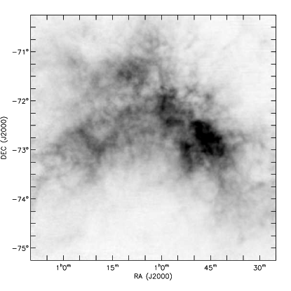
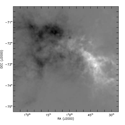
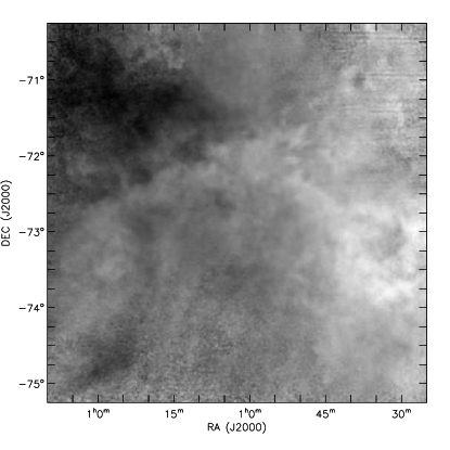
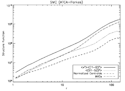
Figure 1: Application to Small Magellanic Cloud observations (data from Stanimirovic et al. 1999.) Top left: column density map. Top right and bottom left: unnormalized velocity centroids and normalized velocity centroids, respectively. Bottom right: structure functions of the maps of column density and centroids (as indicated in the legend).

To illustrate what we describe above, we have taken HI 21 cm. data that combines observations with the Parkes telescope and the Australia Telescope Compact Array (ATCA) interferometer, obtained by Stanimirovic et al. (1999). We obtained from them maps of column density, velocity centroids (normalized and unnormalized), and MVCs, they are shown in Figure 1. From both maps of centroids it is evident the global large scale motion of the SMC, a rotation respect to an axis that forms an angle of $\gtrsim 45\arcdeg$ with respect to the $x$-axis in the maps of the Figure. On top with this regular motion there is an important turbulent velocity field.

We have computed the structure function of these quantities, and we show them in the last panel of Figure 1. For this object $\langle\tilde{S}^{2}\rangle/\langle\tilde{I}^{2}\rangle\sim 0.36$, thus we should expect centroids not to trace the scaling of velocity but rather should be highly affected by density fluctuations. This can be verified from the figure: $I1=\left\langle v^{2}\right\rangle\left\langle(I_{1}-I_{2})^{2}\right\rangle$ (i.e. $\left\langle v^{2}\right\rangle$ times the structure function of column density) is larger than any other quantity plotted, over the entire range of scales. The conclusion of this excercise is that to obtain the spectral index of turbulent velocity in the SMC one should resort to other techniques, such as VCA (see Stanimirović & Lazarian, 2001).

0.4 The effect of magnetic field: anisotropy in structure and correlation functions

Figure 2: Taken from EL05: Anisotropy in the correlation functions: contours of equal correlation for MHD simulations (solid lines). For reference we show isotropic contours as dotted lines. The sonic and Alfvén Mach numbers ($\mathcal{M}_{s}$, $\mathcal{M}_{A}$ respectively), and the plasma $\beta$ are indicated in the title of the plots. The anisotropy reveals the direction of the magnetic field for all the sub-Alfvénic cases, regardless of the sonic Mach number.

Figure 3: Taken from EL05: Correlation functions taken in directions parallel and perpendicular to the mean magnetic field. The anisotropy shows in the different scale-lengths for the distinct directions. It is noticeable the little difference in panels (a), (b), and (d). Which correspond to the same ratio $\tilde{B}/B_{0}$, but very different sonic Mach numbers. Panel (c) corresponds to super-Alfvénic ($\tilde{B}>B_{0}$) turbulence, and the anisotropy is not evident in the centroid maps.

The presence of a magnetic field introduces a preferential direction of motion that makes the turbulent cascade anisotropic. In a magnetized plasma, the eddies become elongated in the direction of their local magnetic field (see for instance Cho, Lazarian, & Vishniac 2002). Fortunately, in spite of being innadequate to recover the spectral index of velocity, velocity centroids reflect the anisotropic cascade in sub-Alfvénic turbulence (regardless of the sonic Mach number). In isotropic turbulence, two-point statistics depend only in the magnitude of the lag (or wave-number), therefore isocontours of 2D two-point statistics are circular. In magnetized turbulence, however, such isocontours become ellipses that are alligned with the mean magnetic field. The magnitude of the magnetic field determines how ellongated they are. Velocity statistics have been proposed before to study this technique (e.g. Esquivel et al. 2003; Vestuto, Ostriker & Stone 2003; EL05), but to our knowledge, they have not been exploited observationally.

In Figure 2 we show (taken from EL05) contours of equal correlation in maps of centroids from MHD simulations with different sonic and Alfvén Mach numbers, as well as different plasma $\beta$ (the ratio of gas to magnetic pressures). The parameters of the simulations are included in the label of each panel, and in more detail in EL05.

It is evident from the Figure the clear anisotropy present in all the sub-Alfvénic cases, regardless of the large differences in sonic Mach numbers and/or plasma $\beta$. The only case in which the anosotropy is not evident is for super-Alfvénic turbulence (panel [c], with $\mathcal{M_{A}}\sim 8$). Whether turbulence in the ISM is typically sub-Alfvénic or super-Alfvénic is an open debate, for instance Padoan et al. (2004) advocate for a model of supersonic turbulence in molecular clouds.

A different way to visualize the anisotropy in two-point statistics is to separate the correlations into perpendicular and parallel to the mean (i.e. global) magnetic field. This would mean to plot the value of the correlations only along the symmetry axes of the ellipses of equal correlation. We present this in Figure 3 (from EL05).

In this case the anisotropy reveals itself as two distinct correlation lenghts for the parallel and perpendicular direction. The difference in scale-lengths should in principle reflect a dependence on $(\tilde{B}/B_{0})^{2}$, where $\tilde{B}$ is the fluctuating magnetic field and $B_{0}$ the mean magnetic field. One should have in mind, however, that this method is only sensitive to the direction of the magnetic field in the plane of the sky. Turbulence with a strong mean magnetic field oriented along the line of sight would be indistinguishable from super-Alfvénic turbulence. It is therefore difficult to determine $(\tilde{B}/B_{0})$ from this type of statistics in supersonic turbulence (where density fluctations are important). Nonetheless, the results in terms of the direction of the $B_{0}$ are robust and could be used when other methods are not available.

0.5 Discussion and Summary

We have made a review of our previous work on velocity centroids, and their application to retrieve the scaling properties of the turbulent velocity field (i.e. spectral index). Additional details can be found in Esquivel et al. (2003); LE03; EL05; OELS06, and Esquivel et al. (2007). This work on centroids assumes a optically thin medium with emissivity proportional to density (e.g. HI), while self absorption has been addressed within VCA (Lazarian & Pogosyan, 2004) and VCS (Lazarian & Pogosyan 2006) techniques, which opens a way of formulating the theory of centroids for partially absorbing media. This has not been done yet.

We also assumed that the emission lines are being used. If the turbulence volume is between the observer and an extended emission source, centroids can be also used with the absorption lines. The present theory assumes that the absorption is in linear regime however. Needless to say, that extend of the emission source of multiple emission sources will determine the spatial coverage of scales that are testable with the centroids. In comparison, the VCS technique can deal with saturated absorption lines and does not depend on the spatial coverage of the data.

The advantage of centroids compared to the VCA and the VCS techniques is, first of all, the ability of centroids to study magnetic field direction, and, second, ability to study subsonic turbulence more reliably. While the VCA and VCS are also capable of studying subsonic turbulence, the procedures for extracting of information within these techniques are much more complicated.

The most frequent mistake, we feel, is the use of centroids while dealing with supersonic data (see Miville-Deschênes et al. 2003). It is important to understand that when we deal with the multi-phase interstellar medium, e.g. HI, the criterion of being subsonic is the most difficult to be satisfied for the cold medium. Therefore, our research shows that while the application of centroids to HII regions is justified, their applications to find the statistics of velocities in molecular clouds and cold HI cannot deliver reliable spectra. This, as we shown, should not discourage the use of the centroids for studies the direction of magnetic field. The reliability of the latter technique can be tested by comparing the polarization arising from aligned dust (see Lazarian & Hoang 2007 for a discussion when we can rely on grain alignment to trace magnetic fields) and the results of the statistical anisotropy analysis with centroids.

The main results of the paper above can be summarized as the following:

• Centroids maps can be used to trace the spectral index of the underyling turbulent velocity in subsonic turbulence. In mildly supersonic turbulence (sonic Mach number $\lesssim 2$ can be studied with MVCs (LE03, EL05).

• Two criteria can be used to determine if centroids are useful to obtain the velocity spectral index. If $\left\langle\left[S(\mathbf{X_{1}})-S(\mathbf{X_{2}})\right]^{2}\right\rangle/I1\ll 1$ (see eqs 8, 9) or if $\sigma_{\rho}/\rho_{0}<1$. The first is a necessary condition, the latter is more robust measure, but might require additional information than what is ussually available from spectroscopic observations.

• We presented an example of the application of velocity centroids to try retrieving the velocity spectral index from real data (SMC observations from Stanimirovic et al. 1999). The criteria proposed above was not fulfilled, thus the spectral index should be studied using an alternate method (such as VCA, see Stanimirović & Lazarian 2001). We showed how the dominant contribution to the statistics of centroids are density fluctuations.

• Two point statistics are anisotropic for sub-Alfvénic turbulence, both for subsonic and supersonic cases. This anisotropy is evident if we plot isocontours of velocity centroids, which become elongated and reveal the direction of the mean magnetic field projected onto the plane of the sky. This anisotropy can be used where other magnetic field measures are not available.

Acknowledgments:

AE acknowledges support from the DGAPA (UNAM) grant IN108207, from the CONACyT grants 46828-F and 61547, and from the “Macroproyecto de Tecnologías para la Universidad de la Información y la Computación” (Secretaría de Desarrollo Institucional de la UNAM). AL acknowledges the support from the NSF grant AST 0808118 and the NSF Center for Magnetic Self-Organization in Astrophysical and Laboratory Plasmas.

References

- Armstrong et al. (1995) Armstrong, J. W., Rickett, B. J., & Spangler, S. R. 1995, ApJ, 443, 209
- Bensch et al. (2001) Bensch, F., Stutzki, J., & Ossenkopf, V. 2001, A&A, 366, 636
- Chepurnov et al. (2008) Chepurnov, A., Gordon, J., Lazarian, A., & Stanimirovic, S. 2008, ApJ, 688, 1021
- Cho & Lazarian (2003) Cho, J., & Lazarian, A. 2003, MNRAS, 345, 325
- Cho & Lazarian (2005) Cho, J., & Lazarian, A. 2005, Theoretical and Computaional Fluid Dynamics, 19, 127
- Cho et al. (2002) Cho, J., Lazarian, A., & Vishniac E. T. 2002, ApJ, 564, 291
- Cho et al. (2003) Cho, J., Lazarian, A., & Vishniac, E. T. 2003, Turbulence and Magnetic Fields in Astrophysics, 614, 56
- Deshpande et al. (2000) Deshpande, A. A., Dwarakanath, K. S., & Goss, W. M. 2000, ApJ, 543, 227
- Dickman & Kleiner (1985) Dickman, R. L., & Kleiner, S. C. 1985, ApJ, 295, 479
- Elmegreen & Scalo (2004) Elmegreen, B. G., & Scalo, J. 2004, ARA&A, 42, 211
- Esquivel et al. (2003) Esquivel, A., Lazarian, A., Pogosyan, D., & Cho, J. 2003, MNRAS, 342, 325
- Esquivel et al. (2007) Esquivel, A., Lazarian, A., Horibe, S., Cho, J., Ossenkopf, V., & Stutzki, J. 2007, MNRAS, 381, 1733
- Esquivel & Lazarian (2005) Esquivel, A., & Lazarian, A. 2005, ApJ, 631, 320 (EL05)
- Heyer & Brunt (2004) Heyer, M. H., & Brunt, C. M. 2004, ApJ, 615, L45
- Kleiner & Dickman (1985) Kleiner, S. C., & Dickman, R. L. 1985, ApJ, 295, 466
- Kim & Park (2007) Kim, S., & Park, C. 2007, ApJ, 663, 244
- Larson (1981) Larson, R. B. 1992, MNRAS, 194, 809
- Larson (1992) Larson, R. B. 1992, MNRAS, 256, 641
- Lazarian (1999) Lazarian, A. 1999, in Plasma Turbulence and Energetic Particles in Astrophysics, Eds.: Michał Ostrowski, Reinhard Schlickeiser, Obserwatorium Astronomiczne, Uniwersytet Jagielloński, Kraków 1999, p. 28-47., 28
- Lazarian (2006) Lazarian, A. 2006, AIPC, 874, 301
- Lazarian (2008) Lazarian, A. 2008, Space Science Reviews, in press (arXiv:0811.0845)
- Lazarian & Cho (2005) Lazarian, A,. & Cho, J. 2005, Physica Scripta, T116,32
- Lazarian & Esquivel (2003) Lazarian, A., & Esquivel, A. 2003, ApJL, 592, L37 (LE03)
- Lazarian & Hoang (2007) Lazarian, A., & Hoang, T. 2007, MNRAS, 378, 910
- Lazarian & Pogosyan (2000) Lazarian, A., & Pogosyan, D. 2000, ApJ, 537, 72
- Lazarian & Pogosyan (2004) Lazarian, A., & Pogosyan, D. 2004, ApJ, 616, 943
- Lazarian & Pogosyan (2006) Lazarian, A., & Pogosyan, D. 2006, ApJ, 652, 1348
- Lazarian & Pogosyan (2008) Lazarian, A., & Pogosyan, D. 2008, ApJ, 686, 350
- Lazarian et al. (2002) Lazarian, A., Pogosyan, D., & Esquivel, A. 2002, in ASP Conf. Ser. 276, Seeing Through the Dust, eds. R. Taylor, T. L. Landecker, & A. G. Willis (San Francisco: ASP),182
- Lazarian et al. (2001) Lazarian, A., Pogosyan, D., Vázquez-Semadeni, E., & Pichardo, B. 2001, ApJ, 555, 130
- Lazio et al. (2004) Lazio, T. J. W., Cordes, J. M., de Bruyn, A. G., & Macquart, J.-P. 2004, New Astronomy Review, 48, 1439
- Mac Low & Ossenkopf (2000) Mac Low, M. M., & Ossenkopf, V. 2000, A&A, 353, 339
- McKee & Ostriker (2007) McKee, C. F., & Ostriker, E. C. 2007, ARA&A, 45, 565
- Miville-Deschênes et al. (2003) Miville-Deschênes, M.-A., Joncas, G., Falgarone, E., & Boulanger, F. 2003, A&A, 411, 109
- Miesch & Bally (1994) Miesch, M. S., & Bally, J. 1994, ApJ, 429, 645
- Münch (1958) Münch, G. 1958, Phys. Rev. Lett., 84, 475
- O’Dell & Castañeda (1987) O’Dell , C. R., & Castañeda, H. O. 1987, ApJ, 317, 686
- Ossenkopf et al. (2006) Ossenkopf, V., Esquivel, A., Lazarian, A., & Stutzki, J. 2006, A&A, 452, 223 (OELS06)
- Ossenkopf & Mac Low (2002) Ossenkopf, V., & Mac Low, M. M. 2002, A&A, 390, 307
- Padoan et al. (2004) Padoan, P., Jimenez, R., Nordlund, Å., & Boldyrev, S. 2004, Phys. Rev. Lett., 92, 191102
- Padoan et al. (2001) Padoan, P., Rosolowsky, E. W., & Goodman A. A. 2001, ApJ, 547, 862
- Rosolowsky et al (1999) Rosolowsky, E. W., Goodman, A. A., Wilner, D. J., & Williams, J. P. 1999, ApJ, 524, 887
- Scalo (1984) Scalo, J. M. 1984, ApJ, 277, 556
- Scalo (1987) Scalo, J. M. 1987, in Hollenbach D. F., Thronson H. A., eds. Interstellar Processes, Reidel, Dordrecht, p. 349
- Stanimirović & Lazarian (2001) Stanimirović, S., & Lazarian, A. 2001, ApJL, 551, L53
- Stanimirovic et al. (1999) Stanimirovic, S., Staveley-Smith, L., Dickey, J. M., Sault, R. J., & Snowden, S. L. 1999, MNRAS, 302, 417
- Stutzki et al. (1998) Stutzki, J., Bensch, F., Heithausen, A., Ossenkopf, V., & Zielinsky, M. 1998, A&A, 336, 697
- Vestuto et al. (2003) Vestuto, J.G., Ostriker, E.C., & Stone, J.M. 2003, ApJ, 590, 858
- von Hoerner (1951) von Hoerner, S. 1951, Z. Astrophys., 30, 17