Low-Complexity Near-ML Decoding of Large Non-Orthogonal STBCs Using PDA

Abstract

Non-orthogonal space-time block codes (STBC) from cyclic division algebras (CDA) having large dimensions are attractive because they can simultaneously achieve both high spectral efficiencies (same spectral efficiency as in V-BLAST for a given number of transmit antennas) as well as full transmit diversity. Decoding of non-orthogonal STBCs with hundreds of dimensions has been a challenge. In this paper, we present a probabilistic data association (PDA) based algorithm for decoding non-orthogonal STBCs with large dimensions. Our simulation results show that the proposed PDA-based algorithm achieves near SISO AWGN uncoded BER as well as near-capacity coded BER (within about 5 dB of the theoretical capacity) for large non-orthogonal STBCs from CDA. We study the effect of spatial correlation on the BER, and show that the performance loss due to spatial correlation can be alleviated by providing more receive spatial dimensions. We report good BER performance when a training-based iterative decoding/channel estimation is used (instead of assuming perfect channel knowledge) in channels with large coherence times. A comparison of the performances of the PDA algorithm and the likelihood ascent search (LAS) algorithm (reported in our recent work) is also presented.

Keywords – Non-orthogonal STBCs, large dimensions, high spectral efficiency, low-complexity near-ML decoding, probabilistic data association.

I Introduction

Multiple-input multiple-output (MIMO) systems that employ non-orthogonal space-time block codes (STBC) from cyclic division algebras (CDA) for arbitrary number of transmit antennas, $N_{t}$, are quite attractive because they can simultaneously provide both full-rate (i.e., $N_{t}$ complex symbols per channel use, which is same as in V-BLAST) as well as full transmit diversity [1]. The $2\times 2$ Golden code is a well known non-orthogonal STBC from CDA for 2 transmit antennas [2]. High spectral efficiencies of the order of tens of bps/Hz can be achieved using large non-orthogonal STBCs. For example, a $16\times 16$ STBC from CDA has 256 complex symbols in it with 512 real dimensions; with 16-QAM and rate-3/4 turbo code, this system offers a high spectral efficiency of 48 bps/Hz. Decoding of non-orthogonal STBCs with such large dimensions, however, has been a challenge. Sphere decoder and its low-complexity variants are prohibitively complex for decoding such STBCs with hundreds of dimensions.

In this paper, we present a probabilistic data association (PDA) based algorithm for decoding large non-orthogonal STBCs from CDA. Key attractive features of this algorithm are its low-complexity and near-ML performance in systems with large dimensions (e.g., hundreds of dimensions). While creating hundreds of dimensions in space alone (e.g., V-BLAST) requires hundreds of antennas, use of non-orthogonal STBCs from CDA can create hundreds of dimensions with just tens of antennas (space) and tens of channel uses (time). Given that 802.11 smart WiFi products with 12 transmit antennas at 2.5 GHz are now commercially available [4] (which establishes that issues related to placement of many antennas and RF/IF chains can be solved in large aperture communication terminals like set-top boxes/laptops), large non-orthogonal STBCs (e.g., $16\times 16$ STBC from CDA) in combination with large dimension near-ML decoding using PDA can enable communications at increased spectral efficiencies of the order of tens of bps/Hz (note that current standards achieve only $<10$ bps/Hz using only up to 4 transmit antennas).

PDA, originally developed for target tracking, is widely used in digital communications [5]-[12]. Particularly, PDA algorithm is a reduced complexity alternative to the a posteriori probability (APP) decoder/detector/equalizer. Near-optimal performance has been demonstrated for PDA-based multiuser detection in CDMA systems [5]-[8]. PDA has been used in the detection of V-BLAST signals with small number of dimensions [10]-[12]. To our knowledge, PDA has not been reported for decoding non-orthogonal STBCs with hundreds of dimensions so far. Our results in this paper can be summarized as follows:

• We adapt the PDA algorithm for decoding non-orthogonal STBCs with large dimensions. With i.i.d fading and perfect CSIR, the algorithm achieves near-SISO AWGN uncoded BER and near-capacity coded BER (within about 5 dB of the theoretical capacity) for $12\times 12$ STBC from CDA, 4-QAM, rate-3/4 turbo code, and 18 bps/Hz.

• Relaxing the perfect CSIR assumption, we report results with a training based iterative PDA decoding/channel estimation scheme. The iterative scheme is shown to be effective with large coherence times.

• Relaxing the i.i.d fading assumption by adopting a spatially correlated MIMO channel model (proposed by Gesbert et al in [18]), we show that the performance loss due to spatial correlation is alleviated by using more receive spatial dimensions for a fixed receiver aperture.

• Finally, the performance of the PDA algorithm is compared with that of the likelihood ascent search (LAS) algorithm we recently presented in [13]-[15]. The PDA algorithm is shown to perform better than the LAS algorithm at low SNRs for higher-order QAM (e.g., 16-QAM), and in the presence of spatial correlation.

II System Model

Consider a STBC MIMO system with multiple transmit and receive antennas. An $(n,p,k)$ STBC is represented by a matrix ${\bf X}_{c}\in{\mathbb{C}}^{n\times p}$, where $n$ and $p$ denote the number of transmit antennas and number of time slots, respectively, and $k$ denotes the number of complex data symbols sent in one STBC matrix. The $(i,j)$th entry in ${\bf X}_{c}$ represents the complex number transmitted from the $i$th transmit antenna in the $j$th time slot. The rate of an STBC is $\frac{k}{p}$. Let $N_{r}$ and $N_{t}=n$ denote the number of receive and transmit antennas, respectively. Let ${\bf H}_{c}\in{\mathbb{C}}^{N_{r}\times N_{t}}$ denote the channel gain matrix, where the $(i,j)$th entry in ${\bf H}_{c}$ is the complex channel gain from the $j$th transmit antenna to the $i$th receive antenna. We assume that the channel gains remain constant over one STBC matrix and vary (i.i.d) from one STBC matrix to the other. Assuming rich scattering, we model the entries of ${\bf H}_{c}$ as i.i.d $\mathcal{C}\mathcal{N}(0,1)$. The received space-time signal matrix, ${\bf Y}_{c}\in{\mathbb{C}}^{N_{r}\times p}$, can be written as

$${\bf Y}_{c}={\bf H}_{c}{\bf X}_{c}+{\bf N}_{c},$$ (1)

where ${\bf N}_{c}\in{\mathbb{C}}^{N_{r}\times p}$ is the noise matrix at the receiver and its entries are modeled as i.i.d $\mathcal{C}\mathcal{N}\big{(}0,\sigma^{2}=\frac{N_{t}E_{s}}{\gamma}\big{)}$, where $E_{s}$ is the average energy of the transmitted symbols, and $\gamma$ is the average received SNR per receive antenna [3], and the $(i,j)$th entry in ${\bf Y}_{c}$ is the received signal at the $i$th receive antenna in the $j$th time-slot. Consider linear dispersion STBCs, where ${\bf X}_{c}$ can be written in the form [3]

$${\bf X}_{c} = \sum_{i=1}^{k}x_{c}^{(i)}{\bf A}_{c}^{(i)},$$ (2)

where $x_{c}^{(i)}$ is the $i$th complex data symbol, and ${\bf A}_{c}^{(i)}\in{\mathbb{C}}^{N_{t}\times p}$ is its corresponding weight matrix. The received signal model in (1) can be written in an equivalent V-BLAST form as

$${\bf y}_{c}\,\,=\,\,\sum_{i=1}^{k}x_{c}^{(i)}\,(\widehat{{\bf H}}_{c}\,{\bf a}_{c}^{(i)})+{\bf n}_{c}\,\,=\,\,\widetilde{{\bf H}}_{c}{\bf x}_{c}+{\bf n}_{c},$$ (3)

where ${\bf y}_{c}\in{\mathbb{C}}^{N_{r}p\times 1}=vec\,({\bf Y}_{c})$, $\widehat{{\bf H}}_{c}\in{\mathbb{C}}^{N_{r}p\times N_{t}p}=({\bf I}\otimes{\bf H}_{c})$, ${\bf a}_{c}^{(i)}\in{\mathbb{C}}^{N_{t}p\times 1}=vec\,({\bf A}_{c}^{(i)})$, ${\bf n}_{c}\in{\mathbb{C}}^{N_{r}p\times 1}=vec\,({\bf N}_{c})$, ${\bf x}_{c}\in{\mathbb{C}}^{k\times 1}$ whose $i$th entry is the data symbol $x_{c}^{(i)}$, and $\widetilde{{\bf H}}_{c}\in{\mathbb{C}}^{N_{r}p\times k}$ whose $i$th column is $\widehat{{\bf H}}_{c}\,{\bf a}_{c}^{(i)}$, $i=1,2,\cdots,k$. Each element of ${\bf x}_{c}$ is an $M$-PAM/$M$-QAM symbol. Let ${\bf y}_{c}$, $\widetilde{{\bf H}}_{c}$, ${\bf x}_{c}$, ${\bf n}_{c}$ be decomposed into real and imaginary parts as:

$${\bf y}_{c}={\bf y}_{I}+j{\bf y}_{Q}, {\bf x}_{c}={\bf x}_{I}+j{\bf x}_{Q},$$

$${\bf n}_{c}={\bf n}_{I}+j{\bf n}_{Q}, \widetilde{{\bf H}}_{c}={\bf H}_{I}+j{\bf H}_{Q}.$$ (4)

Further, we define ${\bf H}_{r}\in{\mathbb{R}}^{2N_{r}p\times 2k}$, ${\bf y}_{r}\in{\mathbb{R}}^{2N_{r}p\times 1}$, ${\bf x}_{r}\in{\mathbb{R}}^{2k\times 1}$, and ${\bf n}_{r}\in{\mathbb{R}}^{2N_{r}p\times 1}$ as

$${\bf H}_{r}=\left(\begin{array}[]{cc}{\bf H}_{I}\hskip 5.69054pt-{\bf H}_{Q}\\ {\bf H}_{Q}\hskip 14.22636pt{\bf H}_{I}\end{array}\right),\hskip 11.38109pt{\bf y}_{r}=[{\bf y}_{I}^{T}\hskip 5.69054pt{\bf y}_{Q}^{T}]^{T},$$ (7)

$$\hskip 11.38109pt{\bf x}_{r}=[{\bf x}_{I}^{T}\hskip 5.69054pt{\bf x}_{Q}^{T}]^{T},\hskip 11.38109pt{\bf n}_{r}=[{\bf n}_{I}^{T}\hskip 5.69054pt{\bf n}_{Q}^{T}]^{T}.$$ (8)

$$\hskip 36.98866pt\left[\begin{array}[]{ccccc}\sum_{i=0}^{n-1}d_{0,i}\,t^{i}&\delta\sum_{i=0}^{n-1}d_{n-1,i}\,\omega_{n}^{i}\,t^{i}&\delta\sum_{i=0}^{n-1}d_{n-2,i}\,\omega_{n}^{2i}\,t^{i}&\cdots&\delta\sum_{i=0}^{n-1}d_{1,i}\,\omega_{n}^{(n-1)i}\,t^{i}\\ \sum_{i=0}^{n-1}d_{1,i}\,t^{i}&\sum_{i=0}^{n-1}d_{0,i}\,\omega_{n}^{i}\,t^{i}&\delta\sum_{i=0}^{n-1}d_{n-1,i}\,\omega_{n}^{2i}\,t^{i}&\cdots&\delta\sum_{i=0}^{n-1}d_{2,i}\,\omega_{n}^{(n-1)i}\,t^{i}\\ \sum_{i=0}^{n-1}d_{2,i}\,t^{i}&\sum_{i=0}^{n-1}d_{1,i}\,\omega_{n}^{i}\,t^{i}&\sum_{i=0}^{n-1}d_{0,i}\,\omega_{n}^{2i}\,t^{i}&\cdots&\delta\sum_{i=0}^{n-1}d_{3,i}\,\omega_{n}^{(n-1)i}\,t^{i}\\ \vdots&\vdots&\vdots&\vdots&\vdots\\ \sum_{i=0}^{n-1}d_{n-2,i}\,t^{i}&\sum_{i=0}^{n-1}d_{n-3,i}\,\omega_{n}^{i}\,t^{i}&\sum_{i=0}^{n-1}d_{n-4,i}\,\omega_{n}^{2i}\,t^{i}&\cdots&\delta\sum_{i=0}^{n-1}d_{n-1,i}\,\omega_{n}^{(n-1)i}t^{i}\\ \sum_{i=0}^{n-1}d_{n-1,i}\,t^{i}&\sum_{i=0}^{n-1}d_{n-2,i}\,\omega_{n}^{i}\,t^{i}&\sum_{i=0}^{n-1}d_{n-3,i}\,\omega_{n}^{2i}\,t^{i}&\cdots&\sum_{i=0}^{n-1}d_{0,i}\,\omega_{n}^{(n-1)i}\,t^{i}\end{array}\right].\hskip 28.45274pt(\mbox{9.a})$$

Now, (3) can be written as

$${\bf y}_{r} = {\bf H}_{r}{\bf x}_{r}+{\bf n}_{r}.$$ (9)

Henceforth, we work with the real-valued system in (9). For notational simplicity, we drop subscripts $r$ in (9) and write

$${\bf y} = {\bf H}^{\prime}{\bf x}+{\bf n},$$ (10)

where ${\bf H}^{\prime}={\bf H}_{r}\in{\mathbb{R}}^{2N_{r}p\times 2k}$, ${\bf y}={\bf y}_{r}\in{\mathbb{R}}^{2N_{r}p\times 1}$, ${\bf x}={\bf x}_{r}\in{\mathbb{R}}^{2k\times 1}$, and ${\bf n}={\bf n}_{r}\in{\mathbb{R}}^{2N_{r}p\times 1}$. We assume that the channel coefficients are known at the receiver but not at the transmitter. Let $\mathbb{A}_{i}$ denote the $M$-PAM signal set from which $x_{i}$ ($i$th entry of ${\bf x}$) takes values, $i=0,\cdots,2k-1$. Now, define a $2k$-dimensional signal space $\mathbb{S}$ to be the Cartesian product of $\mathbb{A}_{0}$ to $\mathbb{A}_{2k-1}$. The ML solution is then given by

$${\bf d}_{ML} = {\mbox{arg min}\atop{{\bf d}\in{\mathbb{S}}}}{\bf d}^{T}({\bf H}^{\prime})^{T}{\bf H}^{\prime}{\bf d}-2{\bf y}^{T}{\bf H}^{\prime}{\bf d},$$ (11)

whose complexity is exponential in $k$.

II-A Full-rate Non-orthogonal STBCs from CDA

We focus on the detection of square (i.e., $n=p=N_{t}$), full-rate (i.e., $k=pn=N_{t}^{2}$), circulant (where the weight matrices ${\bf A}_{c}^{(i)}$’s are permutation type), non-orthogonal STBCs from CDA [1], whose construction for arbitrary number of transmit antennas $n$ is given by the matrix in Eqn.(9.a) given at the bottom of this page. In (9.a), $\omega_{n}=e^{\frac{{\bf j}2\pi}{n}}$, ${\bf j}=\sqrt{-1}$, and $d_{u,v}$, $0\leq u,v\leq n-1$ are the $n^{2}$ data symbols from a QAM alphabet. When $\delta=t=1$, the code in (9.a) is information lossless (ILL), and when $\delta=e^{\sqrt{5}\,{\bf j}}$ and $t=e^{{\bf j}}$, it is of full-diversity and information lossless (FD-ILL) [1]. High spectral efficiencies with large $n$ can be achieved using this code construction. However, since these STBCs are non-orthogonal, ML detection gets increasingly impractical for large $n$. Consequently, a key challenge in realizing the benefits of these large STBCs in practice is that of achieving near-ML performance for large $n$ at low decoding complexities. The BER performance results we report in Sec. IV show that the PDA-based decoding algorithm we propose in the following section essentially meets this challenge.

III Proposed PDA-Based Decoding

In this section, we present the proposed PDA-based decoding algorithm for square QAM. The applicability of the algorithm to any rectangular QAM is straightforward. In the real-valued system model in (10), each entry of ${\bf x}$ belongs to a $\sqrt{M}$-PAM constellation, where $M$ is the size of the original square QAM constellation. Let $b_{i}^{(0)},b_{i}^{(1)},\cdots,b_{i}^{(q-1)}$ denote the $q=\log_{2}(\sqrt{M})$ constituent bits of the $i$th entry $x_{i}$ of ${\bf x}$.

We can write the value of each entry of ${\bf x}$ as a linear combination of its constituent bits as

$$x_{i} = \sum_{j=0}^{q-1}2^{j}\,b_{i}^{(j)},\,\,\,\,\,\,\,\,i=0,1,\cdots,2k-1.$$ (12)

Let ${\bf b}\in\{+1,-1\}^{2qk\times 1}$, defined as

$${\bf b}\,\,\stackrel{{\scriptstyle\triangle}}{{=}}\,\,\left[b_{0}^{(0)}\cdots b_{0}^{(q-1)}b_{1}^{(0)}\cdots b_{1}^{(q-1)}\cdots b_{2k-1}^{(0)}\cdots b_{2k-1}^{(q-1)}\right]^{T},$$ (13)

denote the transmitted bit vector. Defining ${\bf c}\stackrel{{\scriptstyle\triangle}}{{=}}[2^{0}\,2^{1}\cdots 2^{q-1}]$, we can write ${\bf x}$ as

$${\bf x} = ({\bf I}\otimes{\bf c}){\bf b},$$ (14)

where ${\bf I}$ is the $2k\times 2k$ identity matrix. Using (14), we can rewrite (10) as

$${\bf y} = \underbrace{{\bf H}^{\prime}({\bf I}\otimes{\bf c})}_{{\stackrel{{\scriptstyle\triangle}}{{=}}\,\,\bf H}}\,{\bf b}+{\bf n},$$ (15)

where ${\bf H}\in{\mathbb{R}}^{2N_{r}p\times 2qk}$ is the effective channel matrix. Our goal is to obtain $\widehat{{\bf b}}$, an estimate of the ${\bf b}$ vector. For this, we iteratively update the statistics of each bit of ${\bf b}$, as described in the following subsection, for a certain number of iterations, and hard decisions are made on the final statistics to get $\widehat{{\bf b}}$.

III-A Iterative Procedure

The algorithm is iterative in nature, where $2qk$ statistic updates, one for each of the constituent bits, are performed in each iteration. We start the algorithm by initializing the a priori probabilities as $P(b_{i}^{(j)}=+1)=P(b_{i}^{(j)}=-1)=0.5$, $\forall\,i=0,\cdots,2k-1$ and $j=0,\cdots,q-1$. In an iteration, the statistics of the bits are updated sequentially, i.e., the ordered sequence of updates in an iteration is $\big{\{}b_{0}^{(0)},\cdots,b_{0}^{(q-1)},\cdots\cdots,\\ b_{2k-1}^{(0)},\cdots b_{2k-1}^{(q-1)}\big{\}}$. The steps involved in each iteration of the algorithm are derived as follows.

The likelihood ratio of bit $b_{i}^{(j)}$ in an iteration, denoted by $\Lambda_{i}^{(j)}$, is given by

$$\Lambda_{i}^{(j)} \stackrel{{\scriptstyle\triangle}}{{=}} \frac{P\big{(}b_{i}^{(j)}=+1|{\bf y}\big{)}}{P\big{(}b_{i}^{(j)}=-1|{\bf y}\big{)}}$$ (16)

$$= \underbrace{\frac{P\big{(}{\bf y}|b_{i}^{(j)}=+1\big{)}}{P\big{(}{\bf y}|b_{i}^{(j)}=-1\big{)}}}_{\stackrel{{\scriptstyle\triangle}}{{=}}\,\,\beta_{i}^{(j)}}\,\,\underbrace{\frac{P\big{(}b_{i}^{(j)}=+1\big{)}}{P\big{(}b_{i}^{(j)}=-1\big{)}}}_{\stackrel{{\scriptstyle\triangle}}{{=}}\,\,\alpha_{i}^{(j)}}.$$

Denoting the $t$th column of ${\bf H}$ by ${\bf h}_{t}$, we can write (15) as

$${\bf y} = {\bf h}_{qi+j}\,b_{i}^{(j)}+\underbrace{\sum_{l=0}^{2k-1}\sum_{{\stackrel{{\scriptstyle m=0}}{{m\neq q(i-l)+j}}}}^{q-1}{\bf h}_{ql+m}\,b_{l}^{(m)}+{\bf n}}_{\stackrel{{\scriptstyle\triangle}}{{=}}\,\,\widetilde{{\bf n}}},$$ (17)

where $\widetilde{{\bf n}}\in{\mathbb{R}}^{2N_{r}p\times 1}$ is the interference plus noise vector. To calculate $\beta_{i}^{(j)}$, we approximate the distribution of $\widetilde{{\bf n}}$ to be Gaussian, and hence ${\bf y}$ is Gaussian conditioned on $b_{i}^{(j)}$. Since there are $2qk-1$ terms in the double summation in (17), this Gaussian approximation gets increasingly accurate for large $N_{t}$ (note that $k=N_{t}^{2}$). Since a Gaussian distribution is fully characterized by its mean and covariance, we evaluate the mean and covariance of ${\bf y}$ given $b_{i}^{(j)}=+1$ and $b_{i}^{(j)}=-1$. For notational simplicity, let us define $p_{i}^{j+}\stackrel{{\scriptstyle\triangle}}{{=}}P(b_{i}^{(j)}=+1)$ and $p_{i}^{j-}\stackrel{{\scriptstyle\triangle}}{{=}}P(b_{i}^{(j)}=-1)$. It is clear that $p_{i}^{j+}+p_{i}^{j-}=1$.

Let ${\mbox{\boldmath{$\mu$}}}_{i}^{j+}\stackrel{{\scriptstyle\triangle}}{{=}}{\mathbb{E}}({\bf y}|b_{i}^{(j)}=+1)$ and ${\mbox{\boldmath{$\mu$}}}_{i}^{j-}\stackrel{{\scriptstyle\triangle}}{{=}}{\mathbb{E}}({\bf y}|b_{i}^{(j)}=-1)$, where ${\mathbb{E}}(.)$ denotes the expectation operator. Now, from (17), we can write ${\mbox{\boldmath{$\mu$}}}_{i}^{j+}$ as

$${\mbox{\boldmath{$\mu$}}}_{i}^{j+} = {\bf h}_{qi+j}+\sum_{l=0}^{2k-1}\sum_{{\stackrel{{\scriptstyle m=0}}{{m\neq q(i-l)+j}}}}^{q-1}{\bf h}_{ql+m}(2p_{l}^{m+}-1).$$ (18)

Similarly, we can write ${\mbox{\boldmath{$\mu$}}}_{i}^{j-}$ as

$${\mbox{\boldmath{$\mu$}}}_{i}^{j-} = -{\bf h}_{qi+j}+\sum_{l=0}^{2k-1}\sum_{{\stackrel{{\scriptstyle m=0}}{{m\neq q(i-l)+j}}}}^{q-1}{\bf h}_{ql+m}(2p_{l}^{m+}-1)$$ (19)

$$= {\mbox{\boldmath{$\mu$}}}_{i}^{j+}-2{\bf h}_{qi+j}.$$

Next, the $2N_{r}p\times 2N_{r}p$ covariance matrix ${\bf C}_{i}^{j}$ of ${\bf y}$ given $b_{i}^{(j)}$ is given by

$${\bf C}_{i}^{j} = {\mathbb{E}}\bigg{\{}\Big{[}{\bf n}+\sum_{l=0}^{2k-1}\sum_{{\stackrel{{\scriptstyle m=0}}{{m\neq q(i-l)+j}}}}^{q-1}{\bf h}_{ql+m}(b_{l}^{(m)}-2p_{l}^{m+}+1)\Big{]}$$ (20)

$$\Big{[}{\bf n}+\sum_{l=0}^{2k-1}\sum_{{\stackrel{{\scriptstyle m=0}}{{m\neq q(i-l)+j}}}}^{q-1}{\bf h}_{ql+m}(b_{l}^{(m)}-2p_{l}^{m+}+1)\Big{]}^{T}\bigg{\}}.$$

Assuming independence among the constituent bits, we can simplify ${\bf C}_{i}^{j}$ in (20) as

$${\bf C}_{i}^{j}\,=\,\sigma^{2}{\bf I}\,+\sum_{l=0}^{2k-1}\sum_{{\stackrel{{\scriptstyle m=0}}{{m\neq q(i-l)+j}}}}^{q-1}{\bf h}_{ql+m}\,{\bf h}_{ql+m}^{T}\,4p_{l}^{m+}(1-p_{l}^{m+}).$$ (21)

Using the above mean and covariance expressions, we can write the distribution of ${\bf y}$ given $b_{i}^{(j)}=\pm 1$ as

$$P({\bf y}|b_{i}^{(j)}=\pm 1) = \frac{e^{-({\bf y}-{\mbox{\boldmath{$\mu$}}}_{i}^{j\pm})^{T}({\bf C}_{i}^{j})^{-1}({\bf y}-{\mbox{\boldmath{$\mu$}}}_{i}^{j\pm})}}{(2\pi)^{N_{r}p}|{\bf C}_{i}^{j}|^{\frac{1}{2}}}.$$ (22)

Similarly, $P({\bf y}|b_{i}^{(j)}=-1)$ is given by

$$P({\bf y}|b_{i}^{(j)}=-1) = \frac{e^{-({\bf y}-{\mbox{\boldmath{$\mu$}}}_{i}^{j-})^{T}({\bf C}_{i}^{j})^{-1}({\bf y}-{\mbox{\boldmath{$\mu$}}}_{i}^{j-})}}{(2\pi)^{N_{r}p}|{\bf C}_{i}^{j}|^{\frac{1}{2}}}.$$ (23)

Using (22) and (23), $\beta_{i}^{j}$ can be written as

$$\beta_{i}^{j} = \frac{P({\bf y}|b_{i}^{(j)}=+1)}{P({\bf y}|b_{i}^{(j)}=-1)}$$ (24)

$$= e^{-\left(({\bf y}-{\mbox{\boldmath{$\mu$}}}_{i}^{j+})^{T}({\bf C}_{i}^{{j}})^{-1}({\bf y}-{\mbox{\boldmath{$\mu$}}}_{i}^{j+})-({\bf y}-{\mbox{\boldmath{$\mu$}}}_{i}^{j-})^{T}({\bf C}_{i}^{j})^{-1}({\bf y}-{\mbox{\boldmath{$\mu$}}}_{i}^{j-})\right)}.$$

Using $\alpha_{i}^{(j)}$ and $\beta_{i}^{(j)}$, $\Lambda_{i}^{(j)}$ is computed using (16). Now, using the value of $\Lambda_{i}^{(j)}$, the statistics of $b_{i}^{(j)}$ is updated as follows. From (16), and using $P(b_{i}^{(j)}=+1|{\bf y})+P(b_{i}^{(j)}=-1|{\bf y})=1$, we have

$$P(b_{i}^{(j)}=+1|{\bf y})\,=\,\frac{\Lambda_{i}^{(j)}}{1+\Lambda_{i}^{(j)}},$$ (25)

and

$$P(b_{i}^{(j)}=-1|{\bf y}) = \frac{1}{1+\Lambda_{i}^{(j)}}.$$ (26)

As an approximation, dropping the conditioning on ${\bf y}$,

$$P(b_{i}^{(j)}=+1)\,\approx\,\frac{\Lambda_{i}^{(j)}}{1+\Lambda_{i}^{(j)}},$$ (27)

and

$$P(b_{i}^{(j)}=-1) \approx \frac{1}{1+\Lambda_{i}^{(j)}}.$$ (28)

Using the above procedure, we update $P(b_{i}^{(j)}=+1)$ and $P(b_{i}^{(j)}=-1)$ for all $i=0,\cdots,{\small 2k-1}$ and $j=0,\cdots,q-1$ sequentially. This completes one iteration of the algorithm; i.e., each iteration involves the computation of $\alpha_{i}^{(j)}$ and equations (18), (19), (21), (24), (16), (27), and (28) for all $i,j$. The updated values of $P(b_{i}^{(j)}=+1)$ and $P(b_{i}^{(j)}=-1)$ in (27) and (28) for all $i,j$ are fed back to the next iteration. The algorithm terminates after a certain number of such iterations. At the end of the last iteration, hard decision is made on the final statistics to obtain the bit estimate $\widehat{b}_{i}^{(j)}$ as $+1$ if $\Lambda_{i}^{(j)}\geq 1$, and $-1$ otherwise. In coded systems, $\Lambda_{i}^{(j)}$’s are fed as soft inputs to the decoder.

III-B Complexity Reduction

The most computationally expensive operation in computing $\beta_{i}^{(j)}$ is the evaluation of the inverse of the covariance matrix, ${\bf C}_{i}^{j}$, of size $2N_{r}p\times 2N_{r}p$ which requires $O(N_{r}^{3}p^{3})$ complexity, which can be reduced as follows. Define matrix ${\bf D}$ as

$${\bf D} \stackrel{{\scriptstyle\triangle}}{{=}} \sigma^{2}{\bf I}+\sum_{l=0}^{2k-1}\sum_{m=0}^{q-1}{\bf h}_{ql+m}{\bf h}_{ql+m}^{T}4p_{l}^{m+}(1-p_{l}^{m+}).$$ (29)

At the start of the algorithm, with $p_{i}^{j+}$ and $p_{i}^{(j)}$ initialized to 0.5 for all $i,j$, D becomes $\sigma^{2}{\bf I}+{\bf H}{\bf H}^{T}$.

Computation of  ${\bf D}^{-1}$: We note that when the statistics of $b_{i}^{(j)}$ is updated using (27) and (28), the ${\bf D}$ matrix in (29) also changes. A straightforward inversion of this updated ${\bf D}$ matrix would require $O(N_{r}^{3}p^{3})$ complexity. However, we can obtain the ${\bf D}^{-1}$ from the previously available ${\bf D}^{-1}$ in $O(N_{r}^{2}p^{2})$ complexity as follows. Since the statistics of only $b_{i}^{(j)}$ is updated, the new ${\bf D}$ matrix is just a rank one update of the old ${\bf D}$ matrix. Therefore, using the matrix inversion lemma, the new ${\bf D}^{-1}$ can be obtained from the old ${\bf D}^{-1}$ as

$${\bf D}^{-1} \leftarrow {\bf D}^{-1}-\frac{{\bf D}^{-1}{\bf h}_{ni+j}{\bf h}_{ni+j}^{T}{\bf D}^{-1}}{{\bf h}_{ni+j}^{T}{\bf D}^{-1}{\bf h}_{ni+j}+\frac{1}{\eta}},$$ (30)

where

$${\eta} = 4p_{i}^{j+}\big{(}1-p_{i}^{j+}\big{)}-4p_{i,old}^{j+}\big{(}1-p_{i,old}^{j+}\big{)},$$ (31)

where $p_{i}^{j+}$ and $p_{i,old}^{j+}$ are the new $\big{(}$i.e., after the update in (27)$\big{)}$ and (28) $\big{)}$ and old (before the update) values, respectively. It can be seen that both the numerator and denominator in the 2nd term on the RHS of (30) can be computed in $O(N_{r}^{2}p^{2})$ complexity. Therefore, the computation of the new ${\bf D}^{-1}$ using the old ${\bf D}^{-1}$ can be done in $O(N_{r}^{2}p^{2})$ complexity.

Computation of $({\bf C}_{i}^{j})^{-1}$: Using (29) and (21), we can write ${\bf C}_{i}^{j}$ in terms of ${\bf D}$ as

$${\bf C}_{i}^{j} = {\bf D}-4p_{i}^{j+}(1-p_{i}^{j+})\,{\bf h}_{qi+j}\,{\bf h}_{qi+j}^{T}.$$ (32)

We can compute $({\bf C}_{i}^{j})^{-1}$ from ${\bf D}^{-1}$ at a reduced complexity using the matrix inversion lemma, which states that

$$({\bf P}+{\bf Q}{\bf R}{\bf S})^{-1}=\,{\bf P}^{-1}-{\bf P}^{-1}{\bf Q}({\bf R}^{-1}+{\bf S}{\bf P}^{-1}{\bf Q})^{-1}{\bf S}{\bf P}^{-1}.$$ (33)

Substituting ${\bf P}_{2N_{r}p\times 2N_{r}p}={\bf D}$, ${\bf Q}_{2N_{r}p\times 1}={\bf h}_{qi+j}$, ${\bf R}_{1\times 1}=-4p_{i}^{j+}(1-p_{i}^{j+})$, and ${\bf S}_{1\times 2N_{r}p}={\bf h}_{qi+j}^{T}$ in (33), we get

$$({\bf C}_{i}^{j})^{-1}\,\,=\,\,{\bf D}^{-1}-\frac{{\bf D}^{-1}\,{\bf h}_{qi+j}\,{\bf h}_{qi+j}^{T}\,{\bf D}^{-1}}{{\bf h}_{qi+j}^{T}\,{\bf D}^{-1}\,{\bf h}_{qi+j}-\frac{1}{4p_{i}^{j+}(1-p_{i}^{j+})}},$$ (34)

which can be computed in $O(N_{r}^{2}p^{2})$ complexity.

Computation of ${\mbox{\boldmath{$\mu$}}}_{i}^{j+}$ and ${\mbox{\boldmath{$\mu$}}}_{i}^{j-}$: Computation of $\beta_{i}^{(j)}$ involves the computation of ${\mbox{\boldmath{$\mu$}}}_{i}^{j+}$ and ${\mbox{\boldmath{$\mu$}}}_{i}^{j-}$ also. From (19), it is clear that ${\mbox{\boldmath{$\mu$}}}_{i}^{j-}$ can be computed from ${\mbox{\boldmath{$\mu$}}}_{i}^{j+}$ with a computational overhead of only $O(N_{r}p)$. From (18), it can be seen that computing ${\mbox{\boldmath{$\mu$}}}_{i}^{j+}$ would require $O(qN_{r}pk)$ complexity. However, this complexity can be reduced as follows. Define vector ${\bf u}$ as

$${\bf u} \stackrel{{\scriptstyle\triangle}}{{=}} \sum_{l=0}^{2k-1}\sum_{m=0}^{q-1}{\bf h}_{ql+m}\big{(}2p_{l}^{m+}-1\big{)}.$$ (35)

Using (18) and (35), we can write

$${\mbox{\boldmath{$\mu$}}}_{i}^{j+} = {\bf u}+2\big{(}1-p_{i}^{j+}\big{)}{\bf h}_{qi+j}.$$ (36)

u can be computed iteratively at $O(N_{r}p)$ complexity as follows. When the statistics of $b_{i}^{(j)}$ is updated, we can obtain the new ${\bf u}$ from the old ${\bf u}$ as

$${\bf u} \leftarrow {\bf u}+2\big{(}p_{i}^{j+}-p_{i,old}^{j+}\big{)}{\bf h}_{ni+j},$$ (37)

whose complexity is $O(N_{r}p)$. Hence, the computation of ${\mbox{\boldmath{$\mu$}}}_{i}^{j+}$ in (35) and ${\mbox{\boldmath{$\mu$}}}_{i}^{j-}$ in (36) needs $O(N_{r}p)$ complexity. The listing of the proposed PDA algorithm is summarized in the Table-I in the next page.

  Table-I: Proposed PDA-based Algorithm Listing       Initialization

1. $p_{i}^{j+}=p_{i}^{j-}=0.5$,   $\Lambda_{i}^{(j)}=1$,

$\forall i=0,1,\cdots 2k-1,j=0,1,\cdots,q-1$.

2. ${\bf u}={\bf 0},\hskip 2.84526pt{\bf D}^{-1}=\big{(}{\bf H}{\bf H}^{T}+\sigma^{2}{\bf I}\big{)}^{-1}$.

3. $num\_iter$: number of iterations

4. $\kappa=1$;        $\kappa$ is the iteration number

Statistics update in the $\kappa$th iteration

5. for $i$ = 0 to $2k-1$

6. for $j$ = 0 to $q-1$

Update of statistics of bit $b_{i}^{(j)}$

7. ${\mbox{\boldmath{$\mu$}}}_{i}^{j+}\,=\,{\bf u}+2\big{(}1-p_{i}^{j+}\big{)}{\bf h}_{qi+j}$

8. ${\mbox{\boldmath{$\mu$}}}_{i}^{j-}\,=\,{\mbox{\boldmath{$\mu$}}}_{i}^{j+}-2{\bf h}_{qi+j}$

9. $({\bf C}_{i}^{j})^{-1}\,=\,{\bf D}^{-1}-\frac{{\bf D}^{-1}\,{\bf h}_{qi+j}\,{\bf h}_{qi+j}^{T}\,{\bf D}^{-1}}{{\bf h}_{qi+j}^{T}\,{\bf D}^{-1}\,{\bf h}_{qi+j}-\frac{1}{4p_{i}^{j+}(1-p_{i}^{j+})}}$

10. ${\small\beta_{i}^{j}\,=\,e^{-\left(({\bf y}-{\mbox{\boldmath{$\mu$}}}_{i}^{j+})^{T}({\bf C}_{i}^{{j}})^{-1}({\bf y}-{\mbox{\boldmath{$\mu$}}}_{i}^{j+})-({\bf y}-{\mbox{\boldmath{$\mu$}}}_{i}^{j-})^{T}({\bf C}_{i}^{j})^{-1}({\bf y}-{\mbox{\boldmath{$\mu$}}}_{i}^{j-})\right)}}$

11. $p_{i,old}^{j+}\,=\,p_{i}^{j+}$,      $p_{i,old}^{j-}\,=\,p_{i}^{j-}$

12. $\alpha_{i}^{(j)}=\frac{p_{i,old}^{j+}}{p_{i,old}^{j-}}$

13. $\Lambda_{i}^{(j)}=\beta_{i}^{(j)}\alpha_{i}^{(j)}$

14. $p_{i}^{j+}\,=\,\frac{\Lambda_{i}^{(j)}}{1+\Lambda_{i}^{(j)}}$,      $p_{i}^{j-}\,=\,\frac{1}{1+\Lambda_{i}^{(j)}}$

Update of ${\bf u}$ and ${\bf D}^{-1}$

15. ${\bf u}\,\leftarrow\,{\bf u}+2\big{(}p_{i}^{j+}-p_{i,old}^{j+}\big{)}{\bf h}_{qi+j}$

16. ${\eta}\,=\,4p_{i}^{j+}\big{(}1-p_{i}^{j+}\big{)}-4p_{i,old}^{j+}\big{(}1-p_{i,old}^{j+}\big{)}$

17. ${\bf D}^{-1}\,\leftarrow\,{\bf D}^{-1}-\frac{{\bf D}^{-1}{\bf h}_{qi+j}{\bf h}_{qi+j}^{T}{\bf D}^{-1}}{{\bf h}_{qi+j}^{T}{\bf D}^{-1}{\bf h}_{qi+j}+\frac{1}{\eta}}$

18. end;        End of for loop starting at line 5

19. if ($\kappa=num\_iter$) goto line 21

20. $\kappa=\kappa+1$, goto line 5

21. ${\widehat{b}}_{i}^{(j)}=\mbox{sgn}\big{(}\log(\Lambda_{i}^{(j)})\big{)}$

$\forall i=0,1,\cdots,2k-1,\hskip 2.84526ptj=0,1,\cdots,q-1$

22. ${\widehat{x}}_{i}=\sum_{j=0}^{q-1}2^{j}\,{\hat{b}}_{i}^{(j)},\hskip 8.53581pt\forall i=0,1,\cdots,2k-1$

23. Terminate  

III-C Overall Complexity

We need to compute ${\bf H}{\bf H}^{T}$ at the start of the algorithm. This requires $O(qkN_{r}^{2}p^{2})$ complexity. So the computation of the initial ${\bf D}^{-1}$ in line 2 requires $O(qkN_{r}^{2}p^{2})+O(N_{r}^{3}p^{3})$. Based on the complexity reduction in Sec. III-B, the complexity in updating the statistics of one constituent bit (lines 7 to 17) is $O(N_{r}^{2}p^{2})$. So, the complexity for the update of all the $2qk$ constituent bits in an iteration is $O(qkN_{r}^{2}p^{2})$. Since the number of iterations is fixed, the overall complexity of the algorithm is $O(qkN_{r}^{2}p^{2})+O(N_{r}^{3}p^{3})$. For $N_{t}=N_{r}$, since there are $k$ symbols per STBC and $q$ bits per symbol, the overall complexity per bit is $O(p^{2}N_{t}^{2})$.

IV Results and Discussions

In this section, we present the simulated uncoded/coded BER of the PDA algorithm in decoding non-orthogonal STBCs from CDA. Number of iterations in the PDA algorithm is set to $m=10$ in all the simulations.

PDA versus LAS performance with 4-QAM: In Fig. 1, we plot the uncoded BER of the PDA algorithm as a function of average received SNR per rx antenna, $\gamma$, in decoding $4\times 4$, $8\times 8$, $16\times 16$ STBCs from CDA with $N_{t}=N_{r}$ and 4-QAM. Perfect channel state information at the receiver (CSIR) and i.i.d fading are assumed. For the same settings, the performance of the LAS algorithm in [13]-[15] with MMSE initial vector are also plotted for comparison. From Fig. 1, it is seen that

• the BER performance of PDA algorithm improves and approaches SISO AWGN performance as $N_{t}=N_{r}$ is increased; e.g., performance close to within about 1 dB from SISO AWGN performance is achieved at $10^{-3}$ uncoded BER in decoding $16\times 16$ STBC from CDA having 512 real dimensions, and this illustrates the ability of the PDA algorithm to achieve excellent performance at low complexities in large non-orthogonal STBC MIMO.

• with 4-QAM, PDA and LAS algorithms achieve almost the same performance.

Figure 1: Comparison of uncoded BER of PDA and LAS algorithms in decoding $4\times 4$, $8\times 8$, $16\times 16$ ILL STBCs. $N_{t}=N_{r}$, 4-QAM. # iterations $m=10$ for PDA. MMSE initial vector for LAS. BER improves for increasing STBC sizes. With 4-QAM, PDA and LAS algorithms achieve almost the same performance.

PDA versus LAS performance with 16-QAM: Figure 2 presents an uncoded BER comparison between PDA and LAS algorithms for $16\times 16$ STBC from CDA with $N_{t}=Nr=16$ and 16-QAM under perfect CSIR and i.i.d fading. It can be seen that the PDA algorithm performs better at low SNRs than the LAS algorithm. For example, with $8\times 8$ and $16\times 16$ STBCs, at low SNRs (e.g., $<25$ dB for $16\times 16$ STBC), PDA algorithm performs better by about 1 dB compared to LAS algorithm at $10^{-2}$ uncoded BER.

Figure 2: Comparison of uncoded BER of PDA and LAS algorithms in decoding $4\times 4$, $8\times 8$, $16\times 16$ ILL STBCs. $N_{t}=N_{r}$, 16-QAM. # iterations $m=10$ for PDA. MMSE initial vector for LAS. With 16-QAM, PDA performs better than LAS at low SNRs.

Turbo coded BER performance of PDA: Figure 3 shows the rate-3/4 turbo coded BER of the PDA algorithm under perfect CSIR and i.i.d fading for $12\times 12$ ILL STBC with $N_{t}=N_{r}=12$ and 4-QAM, which corresponds to a spectral efficiency of 18 bps/Hz. The theoretical minimum SNR required to achieve 18 bps/Hz spectral efficiency on a $N_{t}=N_{r}=12$ MIMO channel with perfect CSIR and i.i.d fading is 4.3 dB (obtained through simulation of the ergodic capacity formula [3]). From Fig. 3, it is seen that the PDA algorithm is able to achieve vertical fall in coded BER within about 5 dB from the theoretical minimum SNR, which is a good nearness to capacity performance.

Figure 3: Turbo coded BER of the PDA algorithm in decoding $12\times 12$ ILL STBC with $N_{t}=N_{r}$, 4-QAM, rate-3/4 turbo code, 18 bps/Hz and $m=10$ for $i)$ perfect CSIR, and $ii)$ estimated CSIR using 2 iterations between PDA decoding/channel estimation. With perfect CSIR, PDA performs close to within about 5 dB from capacity. With estimated CSIR, performance approaches to that with perfect CSIR with increasing coherence times.

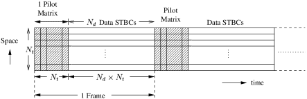
Figure 4: Transmission scheme with one pilot matrix followed by $N_{d}$ data STBC matrices in each frame.

Iterative PDA Decoding/Channel Estimation: We relax the perfect CSIR assumption by considering a training based iterative PDA decoding/channel estimation scheme. Transmission is carried out in frames, where one $N_{t}\times N_{t}$ pilot matrix (for training purposes) followed by $N_{d}$ data STBC matrices are sent in each frame as shown in Fig. 4. One frame length, $T$, (taken to be the channel coherence time) is $T=(N_{d}+1)N_{t}$ channel uses. The proposed scheme works as follows [16]: $i)$ obtain an MMSE estimate of the channel matrix during the pilot phase, $ii)$ use the estimated channel matrix to decode the data STBC matrices using PDA algorithm, and $iii)$ iterate between channel estimation and PDA decoding for a certain number of times. For $12\times 12$ STBC from CDA, in addition to perfect CSIR performance, Fig. 3 also shows the performance with CSIR estimated using the proposed iterative decoding/channel estimation scheme for $N_{d}=1$ and $N_{d}=8$. 2 iterations between decoding and channel estimation are used. With $N_{d}=8$ (which corresponds to large coherence times, i.e., slow fading) the BER and bps/Hz with estimated CSIR get closer to those with perfect CSIR.

Effect of Spatial MIMO Correlation: In Figs. 1 to 3, we assumed i.i.d fading. But spatial correlation at transmit/receive antennas and the structure of scattering and propagation environment can affect the rank structure of the MIMO channel resulting in degraded performance [17]. We relaxed the i.i.d. fading assumption by considering the correlated MIMO channel model in [18], which takes into account carrier frequency ($f_{c}$), spacing between antenna elements ($d_{t},d_{r}$), distance between tx and rx antennas ($R$), and scattering environment. In Fig. 5, we plot the BER of the PDA algorithm in decoding $12\times 12$ STBC from CDA with perfect CSIR in $i)$ i.i.d. fading, and $ii)$ correlated MIMO fading model in [18]. It is seen that, compared to i.i.d fading, there is a loss in diversity order in spatial correlation for $N_{t}=N_{r}=12$; further, use of more rx antennas ($N_{r}=18,N_{t}=12$) alleviates this loss in performance. We can decode perfect codes [19],[20] of large dimensions also using the proposed PDA algorithm.

Figure 5: Effect of spatial correlation on the performance of PDA in decoding $12\times 12$ STBC from CDA. $N_{t}=12$, $N_{r}=12,18$, 16-QAM, rate-3/4 turbo code, 36 bps/Hz. Correlated channel parameters: $f_{c}=5$ GHz, $R=500$ m, $S=30$, $D_{t}=D_{r}=20$ m, $\theta_{t}=\theta_{r}=90^{\circ}$, $N_{r}d_{r}=72$ cm, $d_{t}=d_{r}$. Correlation degrades performance; using $N_{r}>N_{t}$ alleviates the this performance loss.

References

• [1] B. A. Sethuraman, B. S. Rajan, and V. Shashidhar, “Full-diversity high-rate space-time block codes from division algebras,” IEEE Trans. Inform. Theory, vol. 49, no. 10, pp. 2596-2616, October 2003.
• [2] J.-C. Belfiore, G. Rekaya, and E. Viterbo, “The golden code: A $2\times 2$ full-rate space-time code with non-vanishing determinants,” IEEE Trans. Inform. Theory, vol. 51, no. 4, pp. 1432-1436, April 2005.
• [3] H. Jafarkhani, Space-Time Coding: Theory and Practice, Cambridge University Press, 2005.
• [4] http://www.ruckuswireless.com/technology/beamflex.php
• [5] J. Luo, K. Pattipati, P. Willett, and F. Hasegawa, “Near-optimal multiuser detection in synchronous CDMA using probabilistic data association,” IEEE Commun. Letters, vol. 5, no. 9, pp. 361-363, 2001.
• [6] Y. Huang and J. Zhang, “Generalized probabilistic data association multiuser detector,” Proc. ISIT’2004, June-July 2004.
• [7] X. Wang, H. V. Poor, “Iterative (Turbo) soft interference cancellation and decoding for coded CDMA,” IEEE Trans. on Commun., vol. 47, no. 7, pp. 1046-1061, July 1999.
• [8] P. H. Tan and L. K. Rasmussen, “Asymptotically optimal nonlinear MMSE multiuser detection based on multivariate Gaussian approximation,” IEEE Trans. on Commun., vol. 54, no. 8, pp. 1427-1438, August 2006.
• [9] Y. Yin, Y. Huang, and J. Zhang, “Turbo equalization using probabilistic data association,” Proc. IEEE GLOBECOM’2004, vol. 4, pp. 2535-2539, November-December 2004.
• [10] D. Pham, K. R. Pattipati, P. K. Willet, and J. Luo, “A generalized probabilistic data association detector for multiantenna systems,” IEEE Commun. Letters, vol. 8, no. 4, pp. 205-207, 2004.
• [11] G. Latsoudas and N. D. Sidiropoulos, “A hybrid probabilistic data association-sphere decoding for multiple-input-multiple-output systems,” IEEE Sig. Proc. Letters, vol. 12, no. 4, pp. 309-312, April 2005.
• [12] Y. Jia et al, C. M. Vithanage, C. Andrieu, and R. J. Piechocki, “Probabilistic data association for symbol detection in MIMO Systems,” Electronic Letters, vol. 42, no. 1, 5 Jan. 2006.
• [13] K. Vishnu Vardhan, Saif K. Mohammed, A. Chockalingam, B. Sundar Rajan, “A low-complexity detector for large MIMO systems and multicarrier CDMA systems,” IEEE JSAC Spl. Iss. on Multiuser Detection for Adv. Commun. Systems and Networks, vol. 26, no. 3, pp. 473-485, April 2008.
• [14] Saif K. Mohammed, A. Chockalingam, and B. Sundar Rajan “A low-complexity near-ML performance achieving algorithm for large MIMO detection,” Proc. IEEE ISIT’2008, Toronto, Canada, July 2008.
• [15] Saif K. Mohammed, A. Chockalingam, and B. Sundar Rajan, “High-rate space-time coded large MIMO systems: Low-complexity detection and performance,” Proc. IEEE GLOBECOM’2008, New Orleans, USA, Dec. 2008.
• [16] Ahmed Zaki, Saif K. Mohammed, A. Chockalingam, and B. Sundar Rajan, “A training-based iterative detection/channel estimation scheme for large non-orthogonal STBC MIMO systems,” accepted in IEEE ICC’2009, Dresden, Germany, April 2009. Also see arXiv:0809.2446v2 [cs.IT] 4 Oct 2008.
• [17] D. Shiu, G. J. Foschini, M. J. Gans, and J. M. Khan, “Fading correlation and its effect on the capacity of multi-antenna systems,” IEEE Trans. on Commun., vol. 48, pp. 502-513, March 2000.
• [18] D. Gesbert, H. Bölcskei, D. A. Gore, A. J. Paulraj, “Outdoor MIMO wireless channels: Models and performance prediction,” IEEE Trans. on Commun., vol. 50, pp. 1926-1934, December 2002.
• [19] F. E. Oggier, G. Rekaya, J.-C. Belfiore, and E. Viterbo, “Perfect space-time block codes,” IEEE Trans. on Inform. Theory, vol. 52, no. 9, September 2006.
• [20] P. Elia, B. A. Sethuraman, and P. V. Kumar, “Perfect space-time codes for any number of antennas,” IEEE Trans. Inform. Theory, vol. 53, no. 11, pp. 3853-3868, November 2007.