Capacity Achieving Codes From Randomness Condensers

Abstract

We establish a general framework for construction of small ensembles of capacity achieving linear codes for a wide range of (not necessarily memoryless) discrete symmetric channels, and in particular, the binary erasure and symmetric channels. The main tool used in our constructions is the notion of randomness extractors and lossless condensers that are regarded as central tools in theoretical computer science. Same as random codes, the resulting ensembles preserve their capacity achieving properties under any change of basis. Using known explicit constructions of condensers, we obtain specific ensembles whose size is as small as polynomial in the block length. By applying our construction to Justesen’s concatenation scheme (Justesen, 1972) we obtain explicit capacity achieving codes for BEC (resp., BSC) with almost linear time encoding and almost linear time (resp., quadratic time) decoding and exponentially small error probability.

Keywords: Capacity achieving codes, Randomness extractors, Lossless condensers, Code ensembles, Concatenated codes.

I Introduction

One of the basic goals of coding theory is to come up with efficient constructions of error-correcting codes that allow reliable transmission of information over discrete communication channels. Already in the seminal work of Shannon [1], the notion of channel capacity was introduced which is a characteristic of the communication channel that determines the maximum rate at which reliable transmission of information (i.e., with vanishing error probability) is possible. However, Shannon’s result did not focus on the feasibility of the underlying code and mainly concerned with the existence of reliable, albeit possibly complex, coding schemes. Here feasibility can refer to a combination of several criteria, including: succinct description of the code and its efficient computability, the existence of an efficient encoder and an efficient decoder, the error probability, and the set of message lengths for which the code is defined and attains its guaranteed properties.

Besides heuristic attempts, there is a large body of rigorous work in the literature on coding theory with the aim of designing feasible capacity approaching codes for various discrete channels, most notably, the natural and fundamental cases of the binary erasure channel (BEC) and binary symmetric channel (BSC). Some notable examples in “modern coding” include Turbo codes and sparse graph codes (e.g., LDPC codes and Fountain codes, cf. [2, 3, 4]). These classes of codes are either known or strongly believed to contain capacity achieving ensembles for the erasure and symmetric channels.

While such codes are very appealing both theoretically and practically, and are in particular designed with efficient decoding in mind, in this area there still is a considerable gap between what we can prove and what is evidenced by practical results, mainly due to complex combinatorial structure of the code constructions. Moreover, almost all known code constructions in this area involve a considerable amount of randomness, which makes them prone to a possibility of design failure (e.g., choosing an “unfortunate” degree sequence for an LDPC code). While the chance of such possibilities is typically small, in general there is no known efficient way to certify whether a particular outcome of the code construction is satisfactory. Thus, it is desirable to come up with constructions of provably capacity achieving code families that are explicit, i.e., are computationally efficient and do not involve any randomness.

Explicit construction of capacity achieving codes was considered as early as the classic work of Forney [5], who showed that concatenated codes can achieve the capacity of various memoryless channels. In this construction, an outer MDS code is concatenated with an inner code with small block length that can be found in reasonable time by brute force search. An important subsequent work by Justesen [6] (that was originally aimed for explicit construction of asymptotically good codes) shows that it is possible to eliminate the brute force search by varying the inner code used for encoding different symbols of the outer encoding, provided that the ensemble of inner codes contains a large fraction of capacity achieving codes.

Recently, Arıkan [7] gave a framework for deterministic construction of capacity achieving codes for discrete memoryless channels (DMCs) with binary input that are equipped with efficient encoders and decoders and attain slightly worse than exponentially small error probability. These codes are defined for every block length that is a power of two, which might be considered a restrictive requirement. Moreover, the construction is currently explicit (in the sense of polynomial-time computability of the code description) only for the special case of BEC and requires exponential time otherwise.

In this paper, we revisit the concatenation scheme of Justesen and give new constructions of the underlying ensemble of the inner codes. The code ensemble used in Justesen’s original construction is attributed to Wozencraft. Other ensembles that are known to be useful in this scheme include the ensemble of Goppa codes and shortened cyclic codes (see [8], Chapter 12). The number of codes in these ensembles is exponential in the block length and they achieve exponentially small error probability. These ensembles are also known to achieve the Gilbert-Varshamov bound [9, 10], and owe their capacity achieving properties to the property that each nonzero vector belongs to a small number of the codes in the ensemble.

In this work, we will use randomness extractors and lossless condensers that are fundamental objects in theoretical computer science and in particular, theory of pseudorandomness, to construct much smaller ensembles with similar, random-like, properties. The quality of the underlying extractor or condenser determines the quality of the resulting code ensemble. In particular, the size of the code ensemble, the decoding error and proximity to the channel capacity are determined by the seed length, the error, and the output length of the extractor or condenser being used.

As a concrete example, we will instantiate our construction with appropriate choices of the underlying condenser (or extractor) and obtain, for every (sufficiently large) block length $n$, a capacity achieving ensemble of size $2^{n}$ that attains exponentially small error probability for both erasure and symmetric channels (as well as the broader range of channels described above), and an ensemble of quasipolynomial size $2^{O(\log^{3}n)}$ that attains the capacity of BEC. Using nearly optimal extractors and condensers that require logarithmic seed lengths, it is possible to obtain polynomially small capacity achieving ensembles for any block length and this is what we achieve from a lossless condenser due to Guruswami, Umans, and Vadhan [11].

Finally, we apply our constructions to Justesen’s concatenation scheme to obtain an explicit construction of capacity-achieving codes for both BEC and BSC that attain exponentially small error, as in the original construction of Forney. Moreover, the running time of the encoder is almost linear in the block length, and decoding takes almost linear time for BEC and almost quadratic time for BSC. Using our subexponential-sized ensembles as the inner code, we are able to construct explicit codes for BEC and BSC that are defined and capacity achieving for every choice of the message length.

The rest of the paper is organized as follows. In Section II, we review some basic definitions and facts on discrete communication channels and introduce the notion of randomness extractors and condensers that are our main technical tools. In Section III we construct our code ensembles for the binary erasure channel. This is followed by the code ensembles for the binary symmetric and additive noise channels in Section IV. In Section V we incorporate our code ensembles into a code concatenation scheme and construct explicit capacity achieving codes. Finally, Section VI proves a duality theorem for linear affine extractors and condensers that can be seen as a byproduct of the techniques used in the paper, with potential applications of independent interest in the theory of randomness extractors.

II Preliminaries

II-A Discrete Communication Channels

A discrete communication channel is a randomized process that takes a potentially infinite stream of symbols $X_{0},X_{1},\ldots$ from an input alphabet $\Sigma$ and outputs an infinite stream $Y_{0},Y_{1},\ldots$ from an output alphabet $\Gamma$. The indices intuitively represent the time, and each output symbol is only determined from what channel has observed in the past. More precisely, given $X_{0},\ldots,X_{t}$, the output symbol $Y_{t}$ must be independent of $X_{t+1},X_{t+2},\ldots$. In this work, we will concentrate on finite input and finite output channels, that is, when the alphabets $\Sigma$ and $\Gamma$ are finite. In this case, at every time instance $t\in\mathds{N}\cup\{0\}$, the conditional distribution $p(Y_{t}|X_{t})$ of each output symbol $Y_{t}$ given the input symbol $X_{t}$ (and the past outcomes) can be written as a stochastic $|\Sigma|\times|\Gamma|$ transition matrix, where each row is a probability distribution.

Of particular interest is a memoryless channel, which is intuitively “oblivious” of the past. In this case, the transition matrix is independent of the time instance. That is, we have $p(Y_{t}|X_{t})=p(Y_{0}|X_{0})$ for every $t\in\mathds{N}$. When the rows of the transition matrix are permutations of one another and so is the case for the columns, the channel is called symmetric. For example, the channel defined by

$$p(Y|X)=\begin{pmatrix}0.4&0.1&0.5\\ 0.5&0.4&0.1\\ 0.1&0.5&0.4\end{pmatrix}$$

is symmetric. Intuitively, a symmetric channel does not “read” the input sequence. An important class of symmetric channels is defined by additive noise. In an additive noise channel, the input and output alphabets are the same finite field $\mathds{F}_{q}$ and each output symbol $Y_{t}$ is obtained from $X_{t}$ using

$$Y_{t}=X_{t}+Z_{t},$$

where the addition is over $\mathds{F}_{q}$ and the channel noise $Z_{t}\in\mathds{F}_{q}$ is chosen independently of the input sequence. Typically $Z_{t}$ is also independent of time $t$, in which case we get a memoryless additive noise channel. For a noise distribution $\mathcal{Z}$, we denote the memoryless additive noise channel over the input (as well as output) alphabet $\Sigma$ by $\mathsf{SC}(\Sigma,\mathcal{Z})$.

Note that the notion of additive noise channels can be extended to the case where the input and alphabet sets are vector spaces $\mathds{F}_{q}^{n}$, and the noise distribution is a probability distribution over $\mathds{F}_{q}^{n}$. By considering an isomorphism between $\mathds{F}_{q}^{n}$ and the field extension $\mathds{F}_{q^{n}}$, such a channel is essentially an additive noise channel $\mathsf{SC}(\mathds{F}_{q^{n}},\mathcal{Z})$, where $\mathcal{Z}$ is a noise distribution over $\mathds{F}_{q^{n}}$. On the other hand, the channel $\mathsf{SC}(\mathds{F}_{q^{n}},\mathcal{Z})$ can be regarded as a “block-wise memoryless” channel over the alphabet $\mathds{F}_{q}$. Namely, in a natural way, each channel use over the alphabet $\mathds{F}_{q^{n}}$ can be regarded as $n$ subsequent uses of a channel over the alphabet $\mathds{F}_{q}$. When regarding the channel over $\mathds{F}_{q}$, it does not necessarily remain memoryless since the additive noise distribution $\mathcal{Z}$ can be an arbitrary distribution over $\mathds{F}_{q^{n}}$ and is not necessarily expressible as a product distribution over $\mathds{F}_{q}$. However, the noise distributions of blocks of $n$ subsequent channel uses are independent from one another and form a product distribution (since the original channel $\mathsf{SC}(\mathds{F}_{q^{n}},\mathcal{Z})$ is memoryless over $\mathds{F}_{q^{n}}$). Often by choosing larger and larger values of $n$ and letting $n$ grow to infinity, it is possible to obtain good approximations of a non-memoryless additive noise channel using memoryless additive noise channels over large alphabets.

An important additive noise channel is the $q$-ary symmetric channel, which is defined by a (typically small) noise parameter $p\in[0,1-1/q)$. For this channel, the noise distribution $\mathcal{Z}$ has a probability mass $1-p$ on zero, and $p/(q-1)$ on every nonzero alphabet letter. A fundamental special case is the binary symmetric channel (BSC), which corresponds to the case $q=2$ and is denoted by $\mathsf{BSC}(p)$.

Another fundamentally important channel is the binary erasure channel. The input alphabet for this channel is $\{0,1\}$ and the output alphabet is the set $\{0,1,?\}$. The transition is characterized by an erasure probability $p\in[0,1)$. A transmitted symbol is output intact by the channel with probability $1-p$. However, with probability $p$, a special erasure symbol “$?$” is delivered by the channel. The behavior of the binary symmetric channel $\mathsf{BSC}(p)$ and binary erasure channel $\mathsf{BEC}(p)$ is schematically described by Fig. 1.

     

Figure 1: The binary symmetric channel (left) and binary erasure channel (right). On each graph, the left part corresponds to the input alphabet and the right part to the output alphabet. Conditional probability of each output symbol given an input symbol is shown by the labels on the corresponding arrows.

A channel encoder $\mathcal{E}$ for a channel $\mathscr{C}$ with input alphabet $\Sigma$ and output alphabet $\Gamma$ is a mapping $\mathcal{C}\colon\{0,1\}^{k}\to\Sigma^{n}$. A channel decoder, on the other hand, is a mapping $\mathcal{D}\colon\Gamma^{n}\to\{0,1\}^{k}$. A channel encoder and a channel decoder collectively describe a channel code. Note that the image of the encoder mapping defines a block code of length $n$ over the alphabet $\Sigma$. The parameter $n$ defines the block length of the code. For a sequence $Y\in\Sigma^{n}$, denote by the random variable $\mathscr{C}(Y)$ the sequence $\hat{Y}\in\Gamma^{n}$ that is output by the channel, given the input $Y$.

Intuitively, a channel encoder adds sufficient redundancy to a given “message” $X\in\{0,1\}^{k}$ (that is without loss of generality modeled as a binary string of length $k$), resulting in an encoded sequence $Y\in\Sigma^{n}$ that can be fed into the channel. The channel manipulates the encoded sequence and delivers a sequence $\hat{Y}\in\Gamma^{n}$ to a recipient whose aim is to recover $X$. The recovery process is done by applying the channel decoder on the received sequence $\hat{Y}$. The transmission is successful when $\mathcal{D}(\hat{Y})=X$. Since the channel behavior is not deterministic, there might be a nonzero probability, known as the error probability, that the transmission is unsuccessful. More precisely, the error probability of a channel code is defined as

$$p_{e}:=\sup_{X\in\{0,1\}^{k}}\Pr[\mathcal{D}(\mathscr{C}(\mathcal{E}(X)))\neq X],$$

where the probability is taken over the randomness of $\mathscr{C}$. A schematic diagram of a simple communication system consisting of an encoder, point-to-point channel, and decoder is shown in Fig. 2.

Figure 2: The schematic diagram of a point-to-point communication system. The stochastic behavior of the channel is captured by the conditional probability distribution $p(\hat{Y}|Y)$.

For linear codes over additive noise channels, it is often convenient to work with syndrome decoders. Consider a linear code with generator and parity check matrices $G$ and $H$, respectively. The encoding of a message $x$ (considered as a row vector) can thus be written as $xG$. Suppose that the encoded sequence is transmitted over an additive noise channel, which produces a noisy sequence $y:=xG+z$, for a randomly chosen $z$ according to the channel distribution. The receiver receives the sequence $y$ and, without loss of generality, the decoder’s task is to obtain an estimate of the noise realization $z$ from $y$. Now, observe that

$$Hy^{\top}=HG^{\top}x^{\top}+Hz^{\top}=Hz^{\top},$$

where the last equality is due to the orthogonality of the generator and parity check matrices. Therefore, $Hz^{\top}$ is available to the decoder and thus, in order to decode the received sequence, it suffices to obtain an estimate of the noise sequence $z$ from the syndrome $Hz^{\top}$. A syndrome decoder is a function that, given the syndrome, outputs an estimate of the noise sequence (note that this is independent of the codeword being sent). The error probability of a syndrome decoder can be simply defined as the probability (over the noise randomness) that it obtains an incorrect estimate of the noise sequence. Obviously, the error probability of a syndrome decoder upper bounds the error probability of the channel code.

The rate of a channel code (in bits per channel use) is defined as the quantity $k/n$. We call a rate $r\geq 0$ feasible if for every $\epsilon>0$, there is a channel code with rate $r$ and error probability at most $\epsilon$. The rate of a channel code describes its efficiency; the larger the rate, the more information can be transmitted through the channel in a given “time frame”. A fundamental question is, given a channel $\mathscr{C}$, to find the largest possible rate at which reliable transmission is possible. In his fundamental work, Shannon [1] introduced the notion of channel capacity that answers this question. Shannon capacity can be defined using purely information-theoretic terminology. However, for the purposes of this paper, it is more convenient to use the following, more “computational”, definition which turns out to be equivalent to the original notion of Shannon capacity:

$$\mathsf{Cap}(\mathscr{C}):=\sup\{r\mid\text{$r$ is a feasible rate for the channel $\mathscr{C}$}\}.$$

Capacity of memoryless symmetric channels has a particularly nice form. Let $\mathcal{Z}$ denote the probability distribution defined by any of the rows of the transition matrix of a memoryless symmetric channel $\mathscr{C}$ with output alphabet $\Gamma$. Then, capacity of $\mathscr{C}$ is given by

$$\mathsf{Cap}(\mathscr{C})=\log_{2}|\Gamma|-H(\mathcal{Z}),$$

where $H(\cdot)$ denotes the Shannon entropy [12, Section 7.2]. In particular, capacity of the binary symmetric channel $\mathsf{BSC}(p)$ (in bits per channel use) is equal to

$$1-h(p)=1+p\log_{2}p+(1-p)\log_{2}(1-p).$$

Moreover, capacity of the binary erasure channel $\mathsf{BEC}(p)$ is known to be $1-p$ [12, Section 7.1].

A family of channel codes of rate $r$ is an infinite set of channel codes, such that for every (typically small) rate loss $\delta\in(0,r)$ and block length $n$, the family contains a code $\mathcal{C}(n,\delta)$ of length at least $n$ and rate at least $r-\delta$. The family is called explicit if there is a deterministic algorithm that, given $n$ and $\delta$ as parameters, computes the encoder function of the code $\mathcal{C}(n,\delta)$ in polynomial time in $n$. For linear channel codes, this is equivalent to computing a generator or parity check matrix of the code in polynomial time. If, additionally, the algorithm receives an auxiliary index $i\in[s]$, for a size parameter $s$ depending on $n$ and $\delta$, we instead get an ensemble of size $s$ of codes. An ensemble can be interpreted as a set of codes of length $n$ and rate at least $r-\delta$ each, that contains a code for each possibility of the index $i$.

We call a family of codes capacity achieving for a channel $\mathscr{C}$ if the family is of rate $\mathsf{Cap}(\mathscr{C})$ and moreover, the code $\mathcal{C}(n,\delta)$ as described above can be chosen to have an arbitrarily small error probability for the channel $\mathscr{C}$. If the error probability decays exponentially with the block length $n$; i.e., $p_{e}=O(2^{-\gamma n})$, for a constant $\gamma>0$ (possibly depending on the rate loss), then the family is said to achieve an error exponent $\gamma$. We call the family capacity achieving for all lengths if it is capacity achieving and moreover, there is an integer constant $n_{0}$ (depending only on the rate loss $\delta$) such that for every $n\geq n_{0}$, the code $\mathcal{C}(n,\delta)$ can be chosen to have length exactly $n$.

II-B Extractors and Condensers

Extractors and condensers are basic notions in theoretical computer science (and in particular derandomization theory) that constitute the main technical tools that we use for our code constructions. In this section, we review the essential notions and tools related to these objects and probability distributions on finite sample spaces. A detailed treatment of derandomization theory can be found, among other sources, in [15].

The min-entropy of a probability distribution $\mathcal{X}$ over a finite sample space with support $S$ (in symbols, $S:=\mathsf{supp}(\mathcal{X})$) is given by

$$\min_{x\in S}\{-\log\Pr_{\mathcal{X}}(x)\},$$

where $\Pr_{\mathcal{X}}(x)$ is the probability that $\mathcal{X}$ assigns to $x$. All unsubscripted logarithms in this work are to the base $2$ (and thus, the entropy is measured in bits). For a distribution $\mathcal{X}$ over $\mathds{F}_{2}^{n}$, the entropy rate of $\mathcal{X}$ is given by $H_{\infty}(\mathcal{X})/n$.

The statistical distance between two distributions $\mathcal{X}$ and $\mathcal{Y}$ defined on the same finite space $\Omega$ is given by

$$\frac{1}{2}\sum_{s\in\Omega}|\Pr_{\mathcal{X}}(s)-\Pr_{\mathcal{Y}}(s)|,$$

which is half the $\ell_{1}$ distance of the two distributions when regarded as vectors of probabilities over $\Omega$. Two distributions $\mathcal{X}$ and $\mathcal{Y}$ are said to be $\epsilon$-close if their statistical distance is at most $\epsilon$. We will use the shorthand $\mathcal{U}_{n}$ for the uniform distribution on $\mathds{F}_{2}^{n}$, where $\mathds{F}_{2}$ denotes the finite field over $\{0,1\}$, $\mathcal{U}_{S}$ for the uniform distribution on a finite set $S$, and $X\sim\mathcal{X}$ to denote a random variable $X$ drawn from a distribution $\mathcal{X}$.

We will occasionally consider convex combinations of distributions, defined as follows:

Definition 1.

Let $\mathcal{X}_{1},\mathcal{X}_{2},\ldots,\mathcal{X}_{t}$ be probability distributions over a finite space $\Omega$ and $\alpha_{1},\alpha_{2},\ldots,\alpha_{t}$ be nonnegative real values that sum up to $1$. Then the convex combination

$$\alpha_{1}\mathcal{X}_{1}+\alpha_{2}\mathcal{X}_{2}+\cdots+\alpha_{t}\mathcal{X}_{t}$$

is a distribution $\mathcal{X}$ over $\Omega$ given by the probability measure

$$\Pr_{\mathcal{X}}(x):=\sum_{i=1}^{t}\alpha_{i}\Pr_{\mathcal{X}_{i}}(x),$$

for every $x\in\Omega$.

A flat distribution is a distribution that is uniform on its support. For flat distributions, min-entropy coincides with the Shannon-entropy. The set of probability distributions with min-entropy at least $m$ forms a convex set with vertices corresponding to flat distribution with min-entropy $m$ (when $2^{m}$ is an integer). Therefore, any distribution with min-entropy at least $m$ can be written as a convex combination of flat distributions with min-entropy $m$. We will use the following proposition regarding flat probability distributions (a proof is presented in Appendix -A):

Proposition 2.

Let $\mathcal{X}$ be a flat distribution with min-entropy $\log M$ over a finite sample space $\Omega$ and $f\colon\Omega\to\Gamma$ be a mapping to a finite set $\Gamma$.

1. If $f(\mathcal{X})$ is $\epsilon$-close to having min-entropy $\log M$, then there is a set $T\subseteq\Gamma$ of size at least $(1-2\epsilon)M$ such that

   $$(\forall y\in T\text{ and }\forall x,x^{\prime}\in\mathsf{supp}(\mathcal{X}))\colon\\ f(x)=y\land f(x^{\prime})=y\Rightarrow x=x^{\prime}.$$

2. Suppose $|\Gamma|\geq M$. If $f(\mathcal{X})$ has a support of size at least $(1-\epsilon)M$, then it is $\epsilon$-close to having min-entropy $\log M$.

∎

The general notion of randomness condensers that we use in this work is the following:

Definition 3.

A function $f\colon\mathds{F}_{q}^{n}\times\{0,1\}^{d}\to\mathds{F}_{q}^{r}$ is an $m\to_{\epsilon}m^{\prime}$ condenser if for every distribution $\mathcal{X}$ on $\mathds{F}_{q}^{n}$ with min-entropy at least $m$, random variable $X\sim\mathcal{X}$ and a seed $Y\sim\mathcal{U}_{d}$, the distribution of $(Y,f(X,Y))$ is $\epsilon$-close to a distribution $(\mathcal{U}_{d},\mathcal{Z})$ with min-entropy at least $d+m^{\prime}$. The parameters $m$, $m^{\prime}$, $\epsilon$, $m-m^{\prime}$, and $r\log q-m^{\prime}$ are called the input entropy, output entropy, error, the entropy loss and the overhead of the condenser, respectively. A condenser is explicit if it is polynomial-time computable, and linear if it is a linear function in the first argument. That is, when for every fixed seed $z\in\{0,1\}^{d}$, every $x,x^{\prime}\in\mathds{F}_{q}^{n}$ and scalars $\alpha,\beta\in\mathds{F}_{q}$ we have

$$f(\alpha x+\beta x^{\prime},z)=\alpha f(x,z)+\beta f(x^{\prime},z),$$

where the addition is coordinate-wise and over the field $\mathds{F}_{q}$.

In this paper, for the most part, we deal with the binary case, where $q=2$. Two extremal cases of Definition 3 are of particular interest. Namely, when the overhead $r\log q-m^{\prime}$ is zero, the output distribution is close to uniform and the condenser is called an extractor. On the other hand, when the entropy loss $m-m^{\prime}$ is zero, the condenser does not lose any of the source entropy and is therefore called a lossless condenser. We will use the shorthand $(m,\epsilon)$-extractor for an $m\to_{\epsilon}m^{\prime}$ condenser with output length $m^{\prime}$ and $(m,\epsilon$)-lossless condenser for an $m\to_{\epsilon}m$ condenser. For technical reasons, in this work we additionally require $(m,\epsilon)$-lossless condensers to remain $(m^{\prime},\epsilon)$-lossless condensers for every $m^{\prime}\leq m$. All the explicit constructions that we mention and use satisfy this property.

When we have a particular random source in mind, a seedless variation of Definition 3 as follows often becomes useful.

Definition 4.

A function $f\colon\mathds{F}_{q}^{n}\to\mathds{F}_{q}^{m}$ is an $m\to_{\epsilon}m^{\prime}$ condenser for a particular source $\mathcal{X}$ having min-entropy at least $m$ if the distribution $f(\mathcal{X})$ is $\epsilon$-close to a distribution that has min-entropy at least $m^{\prime}$.

The extremal notions of extractors and lossless condensers naturally extend to the seedless definition as well. A standard averaging argument can show that a seeded condenser is in fact an equally good condenser for any source for almost every fixing of the seed. More precisely, we have the following:

Proposition 5.

Let $f\colon\mathds{F}_{q}^{n}\times\{0,1\}^{d}\to\mathds{F}_{q}^{r}$ be an $m\to_{\epsilon}m^{\prime}$ condenser. Consider an arbitrary parameter $\delta>0$ and a source $\mathcal{X}$ with min-entropy $m$ or more. Then, for all but at most a $\delta$ fraction of the choices of $z\in\{0,1\}^{d}$, the function $f(\cdot,z)$ is an $m\to_{\epsilon/\delta}m^{\prime}$ condenser for $\mathcal{X}$. ∎

A seedless function may simultaneously be a condenser for a family of sources. Two important families that we consider in this work are bit-fixing and affine sources. A bit-fixing source of length $n$ with min-entropy $m$ is a distribution of random variables $(X_{1},\ldots X_{n})\in\mathds{F}_{2}^{n}$ such that for some (unknown) set $S\subseteq[n]$ of size $m$, the variables $(X_{i}\colon i\in S)$ are independent and uniformly distributed, and the remaining variables are fixed to arbitrary values. More generally, an affine source over $\mathds{F}_{q}^{n}$ of min-entropy $m\log q$ is a flat distribution supported on an affine translation of some (unknown) $m$-dimensional vector space in $\mathds{F}_{q}^{n}$. An $m\to_{\epsilon}m^{\prime}$ bit-fixing (resp., affine) condenser is a function that is an $m\to_{\epsilon}m^{\prime}$ condenser for any bit-fixing (resp., affine) source with min-entropy at least $m$. Same as before, important special cases include bit-fixing, or affine, extractors and lossless condensers.

The code ensembles that we are going to use in this work are based on linear extractors and lossless condensers. In order to get capacity-achieving code ensembles, we need condensers whose output length $r$ is very close to the input entropy $m$; namely, $|r-m|\leq\alpha m$ for an arbitrarily small constant $\alpha$. Moreover, in order to get explicit code ensembles, we need to instantiate our constructions with explicit condensers. Explicit constructions of condensers that are best suitable for our applications include condensers from the Left-over Hash Lemma, Trevisan’s extractor, and the lossless condenser of Guruswami, Umans, and Vadhan. These constructions are briefly reviewed below.

II-B1 The Leftover Hash Lemma

One of the foremost explicit constructions of linear extractors is given by the Leftover Hash Lemma first stated by Impagliazzo, Levin, and Luby [16]. This extractor achieves an optimal output length $r=m-2\log(1/\epsilon)$ albeit with a substantially large seed length $d=n$. In its general form, the lemma states that any universal family of hash functions can be transformed into an explicit extractor. The universality property required by the hash functions is captured by the following definition.

Definition 6.

A family of functions $\mathcal{H}=\{h_{1},\ldots,h_{D}\}$ where $h_{i}\colon\mathds{F}_{2}^{n}\to\mathds{F}_{2}^{r}$ for $i=1,\ldots,D$ is called universal if, for every fixed choice of $x,x^{\prime}\in\mathds{F}_{2}^{n}$ such that $x\neq x^{\prime}$ and a uniformly random $i\in[D]:=\{1,\ldots,D\}$ we have

$$\Pr_{i}[h_{i}(x)=h_{i}(x^{\prime})]\leq 2^{-r}.$$

One of the basic examples of universal hash families is what we call the linear family, defined as follows. Consider an arbitrary isomorphism $\varphi\colon\mathds{F}_{2}^{n}\to\mathds{F}_{2^{n}}$ between the vector space $\mathds{F}_{2}^{n}$ and the extension field $\mathds{F}_{2^{n}}$, and let $0<r\leq n$ be an arbitrary integer. The linear family $\mathcal{H}_{\mathsf{lin}}$ is the set $\{h_{\alpha}\colon\alpha\in\mathds{F}_{2^{n}}\}$ of size $2^{n}$ that contains a function for each element of the extension field $\mathds{F}_{2^{n}}$. For each $\alpha$, the mapping $h_{\alpha}$ is given by

$$h_{\alpha}(x):=(y_{1},\ldots,y_{r}),\text{ where $(y_{1},\ldots,y_{n}):=\varphi^{-1}(\alpha\cdot\varphi(x))$}.$$

Observe that each function $h_{\alpha}$ can be expressed as a linear mapping from $\mathds{F}_{2}^{n}$ to $\mathds{F}_{2}^{r}$. It is well known and straightforward to see that this family is indeed universal (cf. [17]).

The following is a straightforward generalization of the Leftover Hash Lemma which shows that universal hash families can be used to construct not only extractors, but also lossless condensers. For completeness, we present a proof of this extension of this extension (which is not much different from the original proof) in Appendix -B.

Lemma 7.

(Leftover Hash Lemma) Let $\mathcal{H}=\{h_{i}\colon\mathds{F}_{2}^{n}\to\mathds{F}_{2}^{r}\}_{i\in\mathds{F}_{2}^{d}}$ be a universal family of hash functions with $2^{d}$ elements indexed by binary vectors of length $d$, and define the function $f\colon\mathds{F}_{2}^{n}\times\mathds{F}_{2}^{d}\to\mathds{F}_{2}^{r}$ as $f(x,z):=h_{z}(x)$. Then

1. For every $m,\epsilon$ such that $r\leq m-2\log(1/\epsilon)$, the function $f$ is an $(m,\epsilon)$-extractor, and

2. For every $m,\epsilon$ such that $r\geq m+2\log(1/\epsilon)$, the function $f$ is a lossless $(m,\epsilon)$-condenser.

In particular, by choosing $\mathcal{H}=\mathcal{H}_{\mathsf{lin}}$, it is possible to get explicit extractors and lossless condensers with seed length $d=n$.

II-B2 Trevisan’s Extractor

Another basic example of an explicit extractor is Trevisan’s construction [18]. The extractor is based on “black-box pseudorandom generators” and works by encoding the input using a linear error-correcting code and then carefully puncturing the outcome. Clearly an extractor constructed this way is linear. An improved analysis of the extractor due to Raz et al. results in the following theorem:

Theorem 8.

[19] For all positive integers $n,m$ and real parameter $\epsilon>0$, there is an explicit linear $(m,\epsilon)$-extractor $g\colon\mathds{F}_{2}^{n}\times\mathds{F}_{2}^{d}\to\mathds{F}_{2}^{r}$ with $d=O(\log^{3}(n/\epsilon))$ and $r=m-O(d)$. ∎

II-B3 Lossless Condenser of Guruswami-Umans-Vadhan

To this date, one of the best constructions of lossless condensers for the range of parameters of our interest is due to Guruswami et al. [11]. The condenser is based on error-correcting codes and can be best described as a mapping $\mathds{F}_{q}^{\bar{n}}\times\mathds{F}_{q}\to\mathds{F}_{q}^{\bar{r}}$ over a finite field $\mathds{F}_{q}$ (which for us would be an extension of $\mathds{F}_{2}$). The mapping is depicted in Construction 1. It can be proved [11] that this construction indeed gives a lossless condenser for an appropriate setting of the parameters. Even though in general the mapping is not linear, we observe that for any subfield $\mathds{F}_{\bar{q}}$ of $\mathds{F}_{q}$, the parameter $h$ can be chosen to be an integer power of ${\bar{q}}$. It is straightforward to verify that this restriction does not affect the quality of the condenser, and furthermore, makes the mapping $F_{\bar{q}}$-linear for every fixed seed. Thus, using a standard embedding of $\mathds{F}_{q}$ as an $\mathds{F}_{\bar{q}}$-linear vector space, the condenser can be regarded as a linear function over $\mathds{F}_{\bar{q}}$.

The following result (Theorem 9), proved in [11], summarizes the parameters of the condenser. Combined with the above observation, we can also ensure that the condenser is linear. In particular, for the range of parameters that is of interest in this work, the result gives an $\mathds{F}_{2}$-linear $(m,\epsilon$)-lossless condenser with logarithmic seed length $d=O(\log n)$ and output length $r\leq(1+\alpha)m$, where $\alpha$ is an arbitrarily small positive constant.

Theorem 9.

Let $q$ be a fixed prime power and $\alpha>0$ be an arbitrary constant. Then, for parameters ${\bar{n}}\in\mathds{N}$, $m\leq{\bar{n}}\log q$, and $\epsilon>0$, there is an explicit $(m,\epsilon)$-lossless condenser $f\colon\mathds{F}_{q}^{\bar{n}}\times\{0,1\}^{d}\to\mathds{F}_{q}^{\bar{r}}$ with seed length $d\leq(1+1/\alpha)(\log({\bar{n}}m/\epsilon)+O(1))$ and output length satisfying ${\bar{r}}\log q\leq d+(1+\alpha)m$. Moreover, $f$ is a linear function (over $\mathds{F}_{q}$) for every fixed choice of the seed. ∎

• Given: A random sample $X\sim\mathcal{X}$, where $\mathcal{X}$ is a distribution on $\mathds{F}_{q}^{\bar{n}}$ with min-entropy at least $m$, and a uniformly distributed random seed $Z\sim\mathcal{U}_{\mathds{F}_{q}}$ over $\mathds{F}_{q}$.

• Output: A vector $\mathsf{GUV}(X,Z)$ of length $\bar{r}$ over $\mathds{F}_{q}$.

• Construction: Take any irreducible univariate polynomial $G$ of degree $\bar{n}$ over $\mathds{F}_{q}$, and interpret the input $X$ as the coefficient vector of a random univariate polynomial $F$ of degree $\bar{n}-1$ over $\mathds{F}_{q}$. Then, for an integer parameter $h$, the output is given by

  $$\mathsf{GUV}(X,Z):=(F(Z),F_{1}(Z),\ldots,F_{\bar{r}-1}(Z)),$$

  where we have used the shorthand $F_{i}:=F^{h^{i}}\mod G$.

Construction 1 Guruswami-Umans-Vadhan’s Condenser $\mathsf{GUV}\colon\mathds{F}_{q}^{\bar{n}}\times\mathds{F}_{q}\to\mathds{F}_{q}^{\bar{r}}$.

III Codes for the Binary Erasure Channel

Any code with minimum distance $d$ can tolerate up to $d-1$ erasures in the worst case. Thus, one way to ensure reliable communication over $\mathsf{BEC}(p)$ is to use binary codes with relative minimum distance of about $p$. However, known negative bounds on the rate-distance trade-off (e.g., the sphere packing and MRRW bounds) do not allow the rate of such codes to approach the capacity $1-p$. However, by imposing the weaker requirement that most of the erasure patterns should be recoverable, it is possible to attain the capacity with a positive, but arbitrarily small, error probability (as guaranteed by the definition of capacity).

In this section, we consider a different relaxation that preserves the worst-case guarantee on the erasure patterns; namely we consider ensembles of linear codes with the property that any pattern of up to $p$ erasures must be tolerable by all but a negligible fraction of the codes in the ensemble. This in particular allows us to construct ensembles in which all but a negligible fraction of the codes are capacity achieving for BEC. We remark that since we are only considering linear codes, recoverability from a particular erasure pattern $S\subseteq[n]$ (where $n$ is the block length) is a property of the code and independent of the encoded sequence.

Now we introduce two constructions, which employ linear extractors and lossless condensers as their main ingredients. Throughout this section we denote by $f\colon\mathds{F}_{2}^{n}\times\mathds{F}_{2}^{d}\to\mathds{F}_{2}^{r}$ a linear, lossless condenser for min-entropy $m$ and error $\epsilon$ and by $g\colon\mathds{F}_{2}^{n}\times\mathds{F}_{2}^{d^{\prime}}\to\mathds{F}_{2}^{k}$ a linear extractor for min-entropy $n-m$ and error $\epsilon^{\prime}$. We assume that the errors $\epsilon$ and $\epsilon^{\prime}$ are substantially small. Using this notation, we define the ensembles $\mathcal{F}$ and $\mathcal{G}$ as in Construction 2.

• Ensemble $\mathcal{F}$: Define a code $\mathcal{C}_{u}$ for each seed $u\in\mathds{F}_{2}^{d}$ as follows: Let $H_{u}$ denote the $r\times n$ matrix that defines the linear function $f(\cdot,u)$, i.e., for each $x\in\mathds{F}_{2}^{n}$, $H_{u}\cdot x=f(x,u)$. Then $H_{u}$ is a parity check matrix for $\mathcal{C}_{u}$.

• Ensemble $\mathcal{G}$: Define a code $\mathcal{C}^{\prime}_{u}$ for each seed $u\in\mathds{F}_{2}^{d^{\prime}}$ as follows: Let $G_{u}$ denote the $k\times n$ matrix that defines the linear function $g(\cdot,u)$. Then $G_{u}$ is a generator matrix for $\mathcal{C}^{\prime}_{u}$.

Construction 2 Ensembles $\mathcal{F}$ and $\mathcal{G}$ of error-correcting codes.

Obviously, the rate of each code in $\mathcal{F}$ is at least $1-r/n$. Moreover, we can assume without loss of generality that the rank of each $G_{u}$ is exactly $k$. Thus, each code in $\mathcal{G}$ has rate $k/n$. Lemma 11 below is our main tool in quantifying the erasure decoding capabilities of the two ensembles. Before stating the lemma, we mention a proposition showing that linear condensers applied on affine sources achieve either zero or large errors:

Proposition 10.

Suppose that a distribution $\mathcal{X}$ is uniformly supported on an affine $m$-dimensional subspace over $\mathds{F}_{q}^{n}$. Consider a linear function $f\colon\mathds{F}_{q}^{n}\to\mathds{F}_{q}^{r}$, and define the distribution $\mathcal{Y}$ as $\mathcal{Y}:=f(\mathcal{X})$. Suppose that, for some $\epsilon<1/2$, $\mathcal{Y}$ is $\epsilon$-close to having either min-entropy $r\log q$ or at least $m\log q$. Then, $\epsilon=0$.

Proof.

By linearity, $\mathcal{Y}$ is uniformly supported on an affine subspace $A$ of $\mathds{F}_{q}^{r}$. Let $m^{\prime}\leq r$ be the dimension of this subspace, and observe that $m^{\prime}\leq m$.

First, suppose that $\mathcal{Y}$ is $\epsilon$-close to a distribution with min-entropy $r\log q$; i.e., the uniform distribution on $\mathds{F}_{q}^{r}$. Now, the statistical distance between $\mathcal{Y}$ and the uniform distribution is, by definition,

$$\sum_{x\in A}(q^{-m^{\prime}}-q^{-r})=1-q^{m^{\prime}-r}.$$

Since $\epsilon<1/2$, $q\geq 2$, and $m^{\prime}$ and $r$ are integers, this implies that the distance is greater than $1/2$ (a contradiction) unless $m^{\prime}=r$, in which case it becomes zero. Therefore, the output distribution is exactly uniform over $\mathds{F}_{q}^{r}$.

Now consider the case where $\mathcal{Y}$ is $\epsilon$-close to having min-entropy at least $m\log q$. Considering that $m^{\prime}\leq m$, the definition of statistical distance implies that $\epsilon$ is at least

$$\sum_{x\in A}(q^{-m^{\prime}}-q^{-m})=1-q^{m^{\prime}-m}.$$

Similarly as before, we get that $m^{\prime}=m$, meaning that $\mathcal{Y}$ is precisely a distribution with min-entropy $m\log q$. ∎

Lemma 11.

Let $S\subseteq[n]$ be a set of size at most $m$. Then all but a $3\epsilon$ fraction of the codes in $\mathcal{F}$ and all but a $3\epsilon^{\prime}$ fraction of those in $\mathcal{G}$ can tolerate the erasure pattern defined by $S$.

Proof.

We prove the result for the ensemble $\mathcal{G}$. The argument for $\mathcal{F}$ is similar. Consider a bit-fixing source $\mathcal{S}$ on $\mathds{F}_{2}^{n}$ that is uniform on the coordinates specified by $\bar{S}:=[n]\setminus S$ and fixed to zeros elsewhere. Thus the min-entropy of $\mathcal{S}$ is at least $n-m$, and the distribution $(U,g(\mathcal{S},U))$, where $U\sim\mathcal{U}_{d^{\prime}}$, is $\epsilon^{\prime}$-close to $\mathcal{U}_{d^{\prime}+k}$.

By Proposition 5, for all but a $3\epsilon^{\prime}$ fraction of the choices of $u\in\mathds{F}_{2}^{d^{\prime}}$, the distribution of $g(\mathcal{S},u)$ is $(1/3)$-close to $\mathcal{U}_{k}$. Fix such a $u$. By Proposition 10, the distribution of $g(\mathcal{S},u)$ must in fact be exactly uniform. Thus, the $k\times m$ submatrix of $G_{u}$ consisting of the columns picked by $\bar{S}$ must have rank $k$, which implies that for every $x\in\mathds{F}_{2}^{k}$, the projection of the encoding $x\cdot G_{u}$ to the coordinates chosen by $\bar{S}$ uniquely identifies $x$. ∎

The lemma combined with an simple averaging argument implies the following corollary:

Corollary 12.

Let $\mathcal{S}$ be any distribution on the subsets of $[n]$ of size at most $m$. Then all but a $\sqrt{3\epsilon}$ (resp., $\sqrt{3\epsilon^{\prime}}$) fraction of the codes in $\mathcal{F}$ (resp., $\mathcal{G}$) can tolerate erasure patterns sampled from $\mathcal{S}$ with probability at least $1-\sqrt{3\epsilon}$ (resp., $1-\sqrt{3\epsilon^{\prime}}$), where the probability is taken over the randomness of $\mathcal{S}$ ∎

Note that the result holds irrespective of the distribution $\mathcal{S}$, contrary to the familiar case of $\mathsf{BEC}(p)$ for which the erasure pattern is an i.i.d. (i.e., independent and identically-distributed) sequence. For the case of $\mathsf{BEC}(p)$, the erasure pattern (regarded as its binary characteristic vector in $\mathds{F}_{2}^{n}$) is given by $S:=(S_{1},\ldots,S_{n})$, where the random variables $S_{1},\ldots,S_{n}\in\mathds{F}_{2}$ are i.i.d. and $\Pr[S_{i}=1]=p$. We denote this particular distribution by $\mathcal{B}_{n,p}$, which assigns a nonzero probability to every vector in $\mathds{F}_{2}^{n}$. Thus in this case we cannot directly apply Corollary 12. However, note that $\mathcal{B}_{n,p}$ can be written as a convex combination

$$\mathcal{B}_{n,p}=(1-\gamma)\mathcal{U}_{n,\leq p^{\prime}}+\gamma\mathcal{D},$$ (1)

for $p^{\prime}:=p+\Omega(1)$ that is arbitrarily close to $p$, where $\mathcal{D}$ is an “error distribution” whose contribution $\gamma$ is exponentially small. The distribution $\mathcal{U}_{n,\leq p^{\prime}}$ is the distribution $\mathcal{B}_{n,p}$ conditioned on vectors of weight at most $np^{\prime}$. Corollary 12 applies to $\mathcal{U}_{n,\leq p^{\prime}}$ by setting $m=np^{\prime}$. Moreover, by the convex combination above, the erasure decoding error probability of any code for erasure pattern distributions $\mathcal{B}_{n,p}$ and $\mathcal{U}_{n,\leq p^{\prime}}$ differ by no more than $\gamma$. Therefore, the above result applied to the erasure distribution $\mathcal{U}_{n,\leq p^{\prime}}$ handles the particular case of $\mathsf{BEC}(p)$ with essentially no change in the error probability.

In light of Corollary 12, in order to obtain rates arbitrarily close to the channel capacity, the output lengths of $f$ and $g$ must be sufficiently close to the entropy requirement $m$. More precisely, it suffices to have $r\leq(1+\alpha)m$ and $k\geq(1-\alpha)m$ for arbitrarily small constant $\alpha>0$. The seed length of $f$ and $g$ determine the size of the code ensemble. Moreover, the error of the extractor and condenser determine the erasure error probability of the resulting code ensemble. As achieving the channel capacity is the most important concern for us, we will need to instantiate $f$ (resp., $g$) with a linear lossless condenser (resp., extractor) whose output length is close to $m$. We mention suitable instantiations for each function.

For both functions $f$ and $g$, we can use the explicit extractor and lossless condenser obtained from the Leftover Hash Lemma (Lemma 7), which is optimal in the output length, but requires a large seed, namely, $d=n$. The ensemble resulting this way will thus have size $2^{n}$, but attains a positive error exponent $\delta/2$ for an arbitrary rate loss $\delta>0$. Using an optimal lossless condenser or extractor with seed length $d=\log(n)+O(\log(1/\epsilon))$ and output length close to $m$, it is possible to obtain a polynomially small capacity-achieving ensemble. However, in order to obtain an explicit ensemble of codes, the condenser of extractor being used must be explicit as well.

In the world of linear extractors, we can use Trevisan’s extractor (Theorem 8) to improve the size of the ensemble compared to what obtained from the Leftover Hash Lemma. In particular, Trevisan’s extractor combined with Corollary 12 (using ensemble $\mathcal{G}$) immediately gives the following result:

Corollary 13.

Let $p,c>0$ be arbitrary constants. Then for every integer $n>0$, there is an explicit ensemble $\mathcal{G}$ of linear codes of rate $1-p-o(1)$ such that, the size of $\mathcal{G}$ is quasipolynomial, i.e., $|\mathcal{G}|=2^{O(c^{3}\log^{3}n)}$, and, all but an $n^{-c}=o(1)$ fraction of the codes in the ensemble have error probability at most $n^{-c}$ when used over $\mathsf{BEC}(p)$. ∎

For the ensemble $\mathcal{F}$, on the other hand, we can use the linear lossless condenser of Guruswami et al. that only requires a logarithmic seed (Theorem 9). Using this condenser combined with Corollary 12, we can strengthen the above result as follows:

Corollary 14.

Let $p,c,\alpha>0$ be arbitrary constants. Then for every integer $n>0$, there is an explicit ensemble $\mathcal{F}$ of linear codes of rate $1-p-\alpha$ such that $|\mathcal{G}|=O(n^{c^{\prime}})$ for a constant $c^{\prime}$ only depending on $c,\alpha$. Moreover, all but an $n^{-c}=o(1)$ fraction of the codes in the ensemble have error probability at most $n^{-c}$ when used over $\mathsf{BEC}(p)$. ∎

IV Codes for the Binary Symmetric Channel

The goal of this section is to design capacity achieving code ensembles for the binary symmetric channel $\mathsf{BSC}(p)$. In order to do so, we obtain codes for the general (and not necessarily memoryless) class $\mathsf{SC}(\mathds{F}_{q},\mathcal{Z})$ of symmetric channels, where $\mathcal{Z}$ is any flat distribution or sufficiently close to one. For concreteness, we will focus on the binary case where $q=2$. However, we remark that the results and constructions can readily be extended to any fixed prime power $q$.

Recall that the capacity of $\mathsf{BSC}(\mathcal{Z})$, seen as a binary channel, is $1-h(\mathcal{Z})$ where $h(\mathcal{Z})$ is the entropy rate of $\mathcal{Z}$. The special case $\mathsf{BSC}(p)$ is obtained by setting $\mathcal{Z}=\mathcal{B}_{n,p}$; i.e., the product distribution of $n$ Bernoulli random variables with probability $p$ of being equal to $1$.

The code ensemble that we use for the symmetric channel is the ensemble $\mathcal{F}$, obtained from linear lossless condensers, that we introduced in the preceding section. Thus, we adopt the notation (and parameters) that we used before for defining the ensemble $\mathcal{F}$. Recall that each code in the ensemble has rate at least $1-r/n$. In order to show that the ensemble is capacity achieving, we consider the following brute-force decoder for each code:

Brute-force decoder for code $\mathcal{C}_{u}$: Given a received word $\hat{y}\in\mathds{F}_{2}^{n}$, find a codeword $y\in\mathds{F}_{2}^{n}$ of $\mathcal{C}_{u}$ used and a vector $z\in\mathsf{supp}(\mathcal{Z})$ such that $\hat{y}=y+z$. Output $y$, or an arbitrary codeword if no such pair is found. If there is more than one choice for the codeword $y$, arbitrarily choose one of them.

For each $u\in\mathds{F}_{2}^{d}$, denote by $\mathcal{E}(\mathcal{C}_{u},\mathcal{Z})$ the error probability of the above decoder for code $\mathcal{C}_{u}$ over $\mathsf{BSC}(\mathds{F}_{2},\mathcal{Z})$. The following lemma quantifies this probability:

Lemma 15.

Let $\mathcal{Z}$ be a flat distribution with entropy $m$. Then for at least a $1-2\sqrt{\epsilon}$ fraction of the choices of $u\in\mathds{F}_{2}^{d}$, we have $\mathcal{E}(\mathcal{C}_{u},\mathcal{Z})\leq\sqrt{\epsilon}$.

Proof.

The intuitive idea behind the proof is that lossless condensers act “almost injectively” on the support of any input probability distribution with the prescribed entropy. We will use this property to construct a syndrome decoder for the code ensemble that achieves a sufficiently small error probability.

By Proposition 5, for a $1-2\sqrt{\epsilon}$ fraction of the choices of $u\in\{0,1\}^{d}$, the distribution $\mathcal{Y}:=f(\mathcal{Z},u)$ is $(\sqrt{\epsilon}/2)$-close to having min-entropy at least $m$. Fix any such $u$. We show that the error probability $\mathcal{E}(\mathcal{C}_{u},\mathcal{Z})$ is bounded by $\sqrt{\epsilon}$.

For each $y\in\mathds{F}_{2}^{r}$, define

$$\mathcal{N}(y):=|\{x\in\mathsf{supp}(\mathcal{Z})\colon f(x,u)=y\}|$$

and recall that $f(x,u)=H_{u}\cdot x$, where $H_{u}$ is a parity check matrix for $\mathcal{C}_{u}$. Now suppose that a message is encoded using the code $\mathcal{C}_{u}$ to an encoding $x\in\mathcal{C}_{u}$, and that $x$ is transmitted through the channel. The error probability $\mathcal{E}(\mathcal{C}_{u},\mathcal{Z})$ can be written as

$$\mathcal{E}(\mathcal{C}_{u},\mathcal{Z}) = \Pr_{z\sim\mathcal{Z}}[\exists x^{\prime}\in\mathcal{C}_{u},\exists z^{\prime}\in\mathsf{supp}(\mathcal{Z})\setminus z\colon$$

$$\qquad\qquad x+z=x^{\prime}+z^{\prime}]$$

$$\leq \Pr_{z\sim\mathcal{Z}}[\exists x^{\prime}\in\mathcal{C}_{u},\exists z^{\prime}\in\mathsf{supp}(\mathcal{Z})\setminus z\colon$$

$$\qquad\qquad H_{u}\cdot(x+z)=H_{u}\cdot(x^{\prime}+z^{\prime})]$$

$$= \Pr_{z\sim\mathcal{Z}}[\exists z^{\prime}\in\mathsf{supp}(\mathcal{Z})\setminus z\colon$$

$$\qquad\qquad H_{u}\cdot z=H_{u}\cdot z^{\prime}]$$

$$= \Pr_{z\sim\mathcal{Z}}[\mathcal{N}(H\cdot z)>1]$$

$$= \Pr_{z\sim\mathcal{Z}}[\mathcal{N}(f(x,u))>1],$$ (3)

where $\eqref{eqn:errorProbCollision}$ uses the fact that any codeword of $\mathcal{C}_{u}$ is in the right kernel of $H_{u}$.

By the first part of Proposition 2, there is a set $T\subseteq\mathds{F}_{2}^{r}$ of size at least $(1-\sqrt{\epsilon})|\mathsf{supp}(\mathcal{Z})|$ such that, $\mathcal{N}(y)=1$ for every $y\in T$. Since $\mathcal{Z}$ is uniformly distributed on its support, this combined with (3) immediately implies that $\mathcal{E}(\mathcal{C}_{u},\mathcal{Z})\leq\sqrt{\epsilon}$. ∎

The lemma implies that any linear lossless condenser with entropy requirement $m$ can be used to construct an ensemble of codes such that all but a small fraction of the codes are good for reliable transmission over $\mathsf{BSC}(\mathcal{Z})$, where $\mathcal{Z}$ is an arbitrary flat distribution with entropy at most $m$. Similar to the case of BEC, the seed length determines the size of the ensemble, the error of the condenser bounds the error probability of the decoder, and the output length determines the proximity of the rate to the capacity of the channel. Again, using the condenser given by the Leftover Hash Lemma (Lemma 7), we can obtain a capacity achieving ensemble of size $2^{n}$. Moreover, using the linear lossless condenser of Guruswami et al. (Theorem 9) the ensemble can be made polynomially small (similar to the result given by Corollary 14).

It is not hard to see that the converse of the above result is also true; namely, that any ensemble of linear codes that is universally capacity achieving with respect to any choice of the noise distribution $\mathcal{Z}$ defines a linear lossless condenser. This is spelled out in the lemma below.

Lemma 16.

Let $\{\mathcal{C}_{1},\ldots,\mathcal{C}_{T}\}$ be a binary code ensemble of length $n$ and dimension $n-r$ such that for every flat distribution $\mathcal{Z}$ with min-entropy at most $m$ on $\mathds{F}_{2}^{n}$, all but a $\gamma$ fraction of the codes in the ensemble (for some $\gamma\in[0,1)$) achieve error probability at most $\epsilon$ (under syndrome decoding) when used over $\mathsf{SC}(\mathds{F}_{q^{n}},\mathcal{Z})$. Then the function $f\colon\mathds{F}_{2}^{n}\times[T]\to\mathds{F}_{2}^{r}$ defined as

$$f(x,u):=H_{u}\cdot x,$$

where $H_{u}$ is a parity check matrix for $\mathcal{C}_{u}$, is an $(m,2\epsilon+\gamma)$-lossless condenser.

Proof.

The proof is straightforward using similar arguments as in Lemma 15. Without loss of generality (by a convexity argument), let $\mathcal{Z}$ be a flat distribution with min-entropy $m$, and denote by $D\colon\mathds{F}_{2}^{r}\to\mathds{F}_{2}^{n}$ the corresponding syndrome decoder. Moreover, without loss of generality we have taken the decoder to be a deterministic function. For a randomized decoder, one can fix the internal coin flips so as to preserve the upper bound on its error probability. Now let $u$ be chosen such that $\mathcal{C}_{u}$ achieves an error probability at most $\epsilon$ (we know this is the case for at least $\gamma T$ of the choices of $u$).

Denote by $T\subseteq\mathsf{supp}(\mathcal{Z})$ the set of noise realizations that can potentially confuse the syndrome decoder. Namely,

$$T:=\{z\in\mathsf{supp}(\mathcal{Z})\colon\exists z^{\prime}\in\mathsf{supp}(\mathcal{Z}),z^{\prime}\neq z,H_{u}\cdot z=H_{u}\cdot z^{\prime}\}.$$

Note that, for a random $Z\sim\mathcal{Z}$, conditioned on the event that $Z\in T$, the probability that the syndrome decoder errs on $Z$ is at least $1/2$, since we know that $Z$ can be confused by at least one different noise realization. We can write this more precisely as

$$\Pr_{Z\sim\mathcal{Z}}[D(Z)\neq Z\mid Z\in T]\geq 1/2.$$

Since the error probability of the decoder is upper bounded by $\epsilon$, we conclude that

$$\Pr_{Z\sim\mathcal{Z}}[Z\in T]\leq 2\epsilon.$$

Therefore, the fraction of the elements on support of $\mathcal{Z}$ that collide with some other element under the mapping defined by $H_{u}$ is at most $2\epsilon$. Namely,

$$|\{H_{u}\cdot z\colon z\in\mathsf{supp}(\mathcal{Z})\}|\geq 2^{m}(1-2\epsilon),$$

and this is true for at least $1-\gamma$ fraction of the choices of $u$. Thus, for a uniformly random $U\in[T]$ and $Z\sim\mathcal{Z}$, the distribution of $(U,H_{U}\cdot Z)$ has a support of size at least

$$(1-\gamma)(1-2\epsilon)T2^{m}\geq(1-\gamma-2\epsilon)T2^{m}.$$

By the second part of Proposition 2, we conclude that this distribution is $(2\epsilon+\gamma)$-close to having entropy $m+\log T$ and thus, the function $f$ defined in the statement is a lossless $(m,2\epsilon+\gamma)$-condenser. ∎

By this lemma, any known lower bound on the seed length and the output length of lossless condensers directly translates into lower bounds on the size of the code ensemble and proximity to the capacity that can be obtained from our framework. In particular, it is known [20] that any $(m,\epsilon)$-lossless condenser requires seed length $d=\log(n/\epsilon)+\Omega(1)$ and has to output at least $m+\log(1/\epsilon)+\Omega(1)$ bits. These bounds are tight up to additive constants, and are attained by random functions [20]. Thus, in order to get codes with positive error exponent in our framework (i.e., exponentially small error in the block length), the size of the ensemble must be exponentially large. Moreover, for any constant $c>0$, the existence result of [20] shows that there are lossless condensers that give us ensembles of size $2^{cn}$ and positive error exponent (for all but a $2^{\Omega(n)}$ fraction of the codes in the ensemble).

It is worthwhile to point out that the code ensembles $\mathcal{F}$ and $\mathcal{G}$ discussed in this and the preceding section preserve their erasure and error correcting properties under any change of basis in the ambient space $\mathds{F}_{2}^{n}$, due to the fact that a change of basis applied on any linear condenser results in a linear condenser with the same parameters. This is a property achieved by the trivial, but large, ensemble of codes defined by the set of all $r\times n$ parity check matrices. Observe that no single code can be universal in this sense, and it is inevitable to have a sufficiently large ensemble to attain this property.

The Case $\mathsf{BSC}(p)$

For the special case of $\mathsf{BSC}(p)$, the noise distribution $\mathcal{B}_{n,p}$ is not a flat distribution. Fortunately, similar to the BEC case, we can again use convex combinations to show that the result obtained in Lemma 15 can be extended to this important noise distribution. The main tool that we need is an extension of Lemma 15 to convex combinations with a small number of components.

Suppose that the noise distribution $\mathcal{Z}$ is not a flat distribution but can be written as a convex combination

$$\mathcal{Z}=\alpha_{1}\mathcal{Z}_{1}+\cdots+\alpha_{t}\mathcal{Z}_{t}.$$ (4)

of $t$ flat distributions, where the number $t$ of summands is not too large, and

$$|\mathsf{supp}(\mathcal{Z}_{1})|\geq|\mathsf{supp}(\mathcal{Z}_{2})|\geq\cdots\geq|\mathsf{supp}(\mathcal{Z}_{t})|.$$

For this more general case, we need to slightly tune our brute-force decoder in the way it handles ties. In particular, we now require the decoder to find a codeword $y\in\mathcal{C}_{u}$ and a potential noise vector $z\in\mathsf{supp}(\mathcal{Z})$ that add up to the received word, as before. However, in case more than one matching pair is found, we will require the decoder to choose the one whose noise vector $z$ belongs to the component $\mathcal{Z}_{1},\ldots,\mathcal{Z}_{t}$ with smallest support (i.e., largest index). If the noise vector $z\in\mathsf{supp}(\mathcal{Z}_{i})$ that maximizes the index $i$ is still not unique, the decoder can arbitrarily choose one. Under these conventions, we can now prove the following:

Lemma 17.

Suppose that a noise distribution $\mathcal{Z}$ is as in $\eqref{eqn:noiseConvex}$, where each component $\mathcal{Z}_{i}$ has entropy at most $m$, and the function $f$ defining the ensemble $\mathcal{F}$ is an $(m+1,\epsilon)$-lossless condenser. Then for at least a $1-t(t+1)\sqrt{\epsilon}$ fraction of the choices of $u\in\mathds{F}_{2}^{d}$, the brute-force decoder satisfies $\mathcal{E}(\mathcal{C}_{u},\mathcal{Z})\leq 2t\sqrt{\epsilon}$.

Proof.

For each $1\leq i\leq j\leq t$, we define a flat distribution $\mathcal{Z}_{ij}$ that is uniformly supported on $\mathsf{supp}(\mathcal{Z}_{i})\cup\mathsf{supp}(\mathcal{Z}_{j})$. Observe that each $\mathcal{Z}_{ij}$ has min-entropy at most $m+1$ and thus the function $f$ is a lossless condenser with error at most $\epsilon$ for this source. By Proposition 5 combined with a union bound, for a $1-t(t+1)\sqrt{\epsilon}$ fraction of the choices of $u\in\{0,1\}^{d}$, all $t(t+1)/2$ distributions

$$f(\mathcal{Z}_{ij},u)\colon 1\leq i\leq j\leq t$$

are simultaneously $(\sqrt{\epsilon}/2)$-close to having min-entropy at least $m$. Fix any such $u$.

Consider a random variable $Z$, representing the channel noise, that is sampled from $\mathcal{Z}$ as follows: First choose an index $I\in[t]$ randomly according to the distribution induced by $(\alpha_{1},\ldots,\alpha_{t})$ over the indices, and then sample a random noise $Z\sim\mathcal{Z}_{I}$. Using the same line of reasoning leading to $\eqref{eqn:errorProbCollision}$ in the proof of Lemma 15, the error probability with respect to the code $\mathcal{C}_{u}$ (i.e., the probability that the tuned distance decoder gives a wrong estimate on the noise realization $Z$) can now be bounded as

$$\mathcal{E}(\mathcal{C}_{u},\mathcal{Z})\leq\Pr_{I,Z}[\exists i\in\{I,\ldots,t\},\\ \exists z^{\prime}\in\mathsf{supp}(\mathcal{Z}_{i})\setminus Z\colon f(Z,u)=f(z^{\prime},u)].$$

For $i=1,\ldots,t$, denote by $\mathcal{E}_{i}$ the right hand side probability in the above bound conditioned on the event that $I=i$. Fix any choice of the index $i$. Now it suffices to obtain an upper bound on $\mathcal{E}_{i}$ irrespective of the choice of $i$, since

$$\mathcal{E}(\mathcal{C}_{u},\mathcal{Z})\leq\sum_{i\in[t]}\alpha_{i}\mathcal{E}_{i}.$$

We call a noise realization $z\in\mathsf{supp}(\mathcal{Z}_{i})$ confusable if

$$\exists j\geq i,\exists z^{\prime}\in\mathsf{supp}(\mathcal{Z}_{j})\setminus z\colon f(z,u)=f(z^{\prime},u).$$

That is, a noise realization is confusable if it can potentially cause the brute-force decoder to compute a wrong noise estimate. Our goal is to obtain an upper bound on the fraction of vectors on $\mathsf{supp}(\mathcal{Z}_{i})$ that are confusable.

For each $j\geq i$, we know that $f(\mathcal{Z}_{ij},u)$ is $(\sqrt{\epsilon}/2)$-close to having min-entropy at least $m$. Therefore, by the first part of Proposition 2, the set of confusable elements

$$\{z\in\mathsf{supp}(\mathcal{Z}_{i})\colon\exists z^{\prime}\in\mathsf{supp}(\mathcal{Z}_{j})\setminus z\\ \text{ such that }f(z,u)=f(z^{\prime},u)\}$$

has size at most $\sqrt{\epsilon}|\mathsf{supp}(\mathcal{Z}_{ij})|\leq 2\sqrt{\epsilon}|\mathsf{supp}(\mathcal{Z}_{i})|$ (using the fact that, since $j\geq i$, the support of $\mathcal{Z}_{j}$ is no larger than that of $\mathcal{Z}_{i}$). By a union bound on the choices of $j$, we see that the fraction of confusable elements on $\mathsf{supp}(\mathcal{Z}_{i})$ is at most $2t\sqrt{\epsilon}$. Therefore, $\mathcal{E}_{i}\leq 2t\sqrt{\epsilon}$ and we get the desired upper bound on the error probability of the brute-force decoder. ∎

The result obtained by Lemma 17 can be applied to the channel $\mathsf{BSC}(p)$ by observing that the noise distribution $\mathcal{B}_{n,p}$ can be written as a convex combination

$$\mathcal{B}_{n,p}=\sum_{i=n(p-\eta)}^{n(p+\eta)}\alpha_{i}\mathcal{U}_{n,i}+\gamma\mathcal{D},$$

where $\mathcal{U}_{n,i}$ denotes the flat distribution supported on binary vectors of length $n$ and Hamming weight exactly $i$, and $\mathcal{D}$ is the distribution $\mathcal{B}_{n,p}$ conditioned on the vectors whose Hamming weights lie outside the range $[n(p-\eta),n(p+\eta)]$. The parameter $\eta>0$ can be chosen as an arbitrarily small real number, so that the min-entropies of the distributions $\mathcal{U}_{n,i}$ become arbitrarily close to the Shannon entropy of $\mathcal{B}_{n,p}$; namely, $nh(p)$. This can be seen by the estimate

$$\binom{n}{w}=2^{nh(w/n)\pm o(n)},$$

$h(\cdot)$ being the binary entropy function, that is easily derived from Stirling’s formula. By Chernoff bounds, the error $\gamma$ can be upper bounded as

$$\gamma=\Pr_{Z\sim\mathcal{B}_{n,p}}[|\mathsf{wgt}(Z)-np|>\eta n]\leq 2e^{-c_{\eta}np}=2^{-\Omega(n)},$$

where $c_{\eta}>0$ is a constant only depending on $\eta$, and is thus exponentially small. Thus the error probability attained by any code under noise distributions $\mathcal{B}_{n,p}$ and $\mathcal{Z}:=\sum_{i=n(p-\eta)}^{n(p+\eta)}\alpha_{i}\mathcal{U}_{n,i}$ differ by the exponentially small quantity $\gamma$. We may now apply Lemma 17 on the noise distribution $\mathcal{Z}$ to attain code ensembles for the binary symmetric channel $\mathsf{BSC}(p)$. The error probability of the ensemble is at most $2n\sqrt{\epsilon}$, and this bound is satisfied by at least a $1-n^{2}\sqrt{\epsilon}$ fraction of the codes.

Finally, the code ensemble is capacity achieving for $\mathsf{BSC}(p)$ provided that the condenser $f$ attains an output length $r\leq(1+\alpha)(p+\eta)n$ for arbitrarily small constant $\alpha$, and $\epsilon=o(n^{-4})$. Same as before, the required bounds on the output length and error are in particular attained by the Leftover Hash Lemma (Lemma 7) and the lossless condenser of Guruswami et al. (Theorem 9). The parameters achieved by the resulting explicit ensembles are summarized in the table below. These are essentially the same as what we could get for the BEC and $\mathsf{BSC}(\mathcal{Z})$ channels before.

Condenser used	Ensemble size	Error probability
Lemma 7	$2^{n}$	$2^{-\Omega(n)}$
Theorem 9	${\mathsf{poly}}(n)$	$n^{-c}\ (\forall c>0)$

V Explicit Capacity Achieving Codes

In the preceding sections, we showed how to obtain small ensembles of explicit capacity achieving codes for various discrete channels, including the important special cases $\mathsf{BEC}(p)$ and $\mathsf{BSC}(p)$. Two drawbacks related to these constructions are:

1. While an overwhelming fraction of the codes in the ensemble are capacity achieving, in general it is not clear how to pin down a single, capacity achieving code in the ensemble.

2. For the symmetric additive noise channels, the brute-force decoder is extremely inefficient and is of interest only for proving that the constructed ensembles are capacity achieving.

In a classic work, Justesen [6] showed that the idea of code concatenation first introduced by Forney [5] can be used to transform any ensemble of capacity achieving codes, for a memoryless channel, into an explicit, efficiently decodable code with improved error probability over the same channel. In this section we revisit this idea and apply it to our ensembles. For concreteness, we focus on the binary case and consider a memoryless channel $\mathscr{C}$ that is either $\mathsf{BEC}(p)$ or $\mathsf{BSC}(p)$.

Throughout this section, we consider an ensemble $\mathcal{S}$ of linear codes with block length $n$ and rate $R$, for which it is guaranteed that all but a $\gamma=o(1)$ fraction of the codes are capacity achieving (for a particular discrete memoryless symmetric channel, in our case either $\mathsf{BEC}(p)$ or $\mathsf{BSC}(p)$) with some vanishing error probability $\eta=o(1)$ (the asymptotics are considered with respect to the block length $n$).

Justesen’s concatenated codes take an outer code $\mathcal{C}_{\mathrm{out}}$ of block length $s:=|\mathcal{S}|$, alphabet $\mathds{F}_{2^{k}}$, rate $R^{\prime}$ as the outer code. The particular choice of the outer code in the original construction is Reed-Solomon codes. However, we point out that any outer code that allows unique decoding of some constant fraction of errors at rates arbitrarily close to one would suffice for the purpose of constructing capacity achieving codes. In particular, in this section we will use an expander-based construction of asymptotically good codes due to Spielman [21], from which the following theorem can be easily derived:

Theorem 18.

For every integer $k>0$ and every absolute constant $R^{\prime}<1$, there is an explicit family of $\mathds{F}_{2}$-linear codes over $\mathds{F}_{2^{k}}$ for every block length and rate $R^{\prime}$ that is error-correcting for an $\Omega(1)$ fraction of errors. The running time of the encoder and the decoder is linear in the bit-length of the codewords.

V-A Justesen’s Concatenation Scheme

The concatenation scheme of Justesen differs from traditional concatenation in that the outer code is concatenated with an ensemble of codes rather than a single inner code.

In this construction, size of the ensemble is taken to be matching with the block length of the outer code, and each symbol of the outer code is encoded with one of the inner codes in the ensemble. We use the notation $\mathcal{C}:=\mathcal{C}_{\mathrm{out}}\diamond\mathcal{S}$ to denote concatenation of an outer code $\mathcal{C}_{\mathrm{out}}$ with the ensemble $\mathcal{S}$ of inner codes. Suppose that the alphabet size of the outer code is taken to be $2^{\lfloor Rn\rfloor}$, where we recall that $n$ and $R$ denote the block length and rate of the inner codes in $\mathcal{S}$.

The encoding of a message with the concatenated code can be obtained as follows: First, the message is encoded using $\mathcal{C}_{\mathrm{out}}$ to obtain an encoding $(c_{1},\ldots,c_{s})\in\mathds{F}_{2^{k}}^{s}$, where $k=\lfloor Rn\rfloor$ denotes the dimension of the inner codes. Then, for each $i\in[s]$, the $i$th symbol of the encoding $c_{i}$ is further encoded by the $i$th code in the ensemble $\mathcal{S}$ (under some arbitrary ordering of the codes in the ensemble), resulting in a binary sequence $c^{\prime}_{i}$ of length $n$. The $ns$-bit long binary sequence $(c^{\prime}_{1},\ldots,c^{\prime}_{s})$ defines the encoding of the message under $\mathcal{C}_{\mathrm{out}}\diamond\mathcal{S}$. The concatenation is scheme is depicted in Fig. 3.

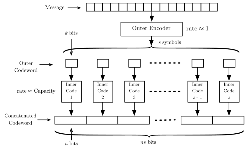
Figure 3: Justesen’s concatenation scheme.

Similar to classical concatenated codes, the resulting binary code $\mathcal{C}$ has block length $N:=ns$ and dimension $K:=kk^{\prime}$, where $k^{\prime}$ is the dimension of the outer code $\mathcal{C}_{\mathrm{out}}$. However, the neat idea in Justesen’s concatenation is that it eliminates the need for a brute-force search for finding a good inner code, as long as almost all inner codes are guaranteed to be good.

V-B The Analysis

In order to analyze the error probability attained by the concatenated code $\mathcal{C}_{\mathrm{out}}\diamond\mathcal{S}$, we consider the following naive decoder:

1. Given a received sequence $(y_{1},\ldots,y_{s})\in(\mathds{F}_{2}^{n})^{s}$, apply an appropriate decoder for the inner codes (e.g., the brute-force decoder for BSC, or Gaussian elimination for BEC) to decode each $y_{i}$ to a codeword $c^{\prime}_{i}$ of the $i$th code in the ensemble.

2. Apply the outer code decoder on $(c^{\prime}_{1},\ldots,c^{\prime}_{s})$ that is guaranteed to correct some constant fraction of errors, to obtain a codeword $(c_{1},\ldots,c_{s})$ of the outer code $\mathcal{C}_{\mathrm{out}}$.

3. Recover the decoded sequence from the corrected encoding $(c_{1},\ldots,c_{s})$.

Since the channel is assumed to be memoryless, the noise distributions on inner codes are independent. Let $\mathcal{G}\subseteq[s]$ denote the set of coordinate positions corresponding to “good” inner codes in $\mathcal{S}$ that achieve an error probability bounded by $\eta$. By assumption, we have $\mathcal{G}\geq(1-\gamma)|\mathcal{S}|$.

Suppose that the outer code $\mathcal{C}_{\mathrm{out}}$ corrects some $\gamma+\alpha$ fraction of adversarial errors, for a constant $\alpha>\eta$. Then an error might occur only if more than $\alpha N$ of the codes in $\mathcal{G}$ fail to obtain a correct decoding. We expect the number of failures within the good inner codes to be $\eta|\mathcal{G}|$. Due to the noise independence, it is possible to show that the fraction of failures may deviate from the expectation $\eta$ only with a negligible probability. In particular, a direct application of the Chernoff bounds implies that the probability that more than an $\alpha$ fraction of the good inner codes err is at most

$$\eta^{\alpha^{\prime}|\mathcal{G}|}=2^{-\Omega_{\alpha}(\log(1/\eta)s)},$$ (5)

where $\alpha^{\prime}>0$ is a constant that only depends on $\alpha$. This also upper bounds the error probability of the concatenated code. In particular, we see that if the error probability $\eta$ of the inner codes is exponentially small in their block length $n$, the concatenated code also achieves an exponentially small error in its block length $N$.

Now we analyze the encoding and decoding complexity of the concatenated code, assuming that Spielman’s expander codes (Theorem 18) are used for the outer code. With this choice, the outer code becomes equipped with a linear-time encoder and decoder. Since any linear code can be encoded in quadratic time (in its block length), the concatenated code can be encoded in $O(n^{2}s)$, which for $s\gg n$ can be considered “almost linear” in the block length $N=ns$ of $\mathcal{C}$. The decoding time of each inner code is cubic in $n$ for the erasure channel, since decoding reduces to Gaussian elimination, and thus for this case the naive decoder runs in time $O(n^{3}s)$.

For the symmetric channel, however, the brute-force decoder used for the inner codes takes exponential time in the block length, namely, $2^{Rn}{\mathsf{poly}}(n)$. Therefore, the running time of the decoder for concatenated code becomes bounded by $O(2^{Rn}s{\mathsf{poly}}(n))$. When the inner ensemble is exponentially large; i.e., $s=2^{n}$ (which is the case for our ensembles if we use the Leftover Hash Lemma), the decoding complexity becomes $O(s^{1+R}{\mathsf{poly}}(\log s))$ which is at most quadratic in the block length of $\mathcal{C}$.

Since the rate $R^{\prime}$ of the outer code can be made arbitrarily close to $1$ (while keeping the minimum distance linear), rate of the concatenated code $\mathcal{C}$ can be made arbitrarily close to the rate $R$ of the inner codes. Thus, if the ensemble of inner codes is capacity-achieving, so would be the concatenated code.

V-C Density of the Explicit Family

In the preceding section we saw how to obtain explicit capacity achieving codes from capacity achieving code ensembles using concatenation. One of the important properties of the resulting family of codes that is influenced by the size of the inner code ensemble is the set of block lengths $N$ for which the concatenated code is defined. Recall that $N=ns$, where $n$ and $s$ respectively denote the block length of the inner codes and the size of the code ensemble, and the parameter $s$ is a function of $n$. For instance, for all classical examples of capacity achieving code ensembles (namely, Wozencraft’s ensemble, Goppa codes and shortened cyclic codes) we have $s(n)=2^{n}$. In this case, the resulting explicit family of codes would be defined for integer lengths of the form $N(i)=i2^{i}$.

A trivial approach for obtaining capacity achieving codes for all lengths is to use a padding trick. Suppose that we wish to transmit a particular bit sequence of length $K$ through the channel using the concatenated code family of rate $\rho$ that is taken to be sufficiently close to the channel capacity. The sequence might originate from a source that does not produce a constant stream of bits (e.g., consider a terminal emulator that produces data only when user input is available).

Ideally, one requires the length of the encoded sequence to be $N=\lceil K/\rho\rceil$. However, since the family might not be defined for the block length $N$, we might be forced to take a code $\mathcal{C}$ in the family with smallest length $N^{\prime}\geq N$ that is of the form $N^{\prime}=ns(n)$, for some integer $n$, and pad the original message with redundant symbols. This way we have encoded a sequence of length $K$ to one of length $N^{\prime}$, implying an effective rate $K/N^{\prime}$. The rate loss incurred by padding is thus equal to $\rho-K/N^{\prime}=K(1/N-1/N^{\prime})$. Thus, if $N^{\prime}\geq N(1+\delta)$ for some positive constant $\delta>0$, the rate loss becomes lower bounded by a constant and subsequently, even if the original concatenated family is capacity achieving, it no longer remains capacity achieving when extended to arbitrarily chosen lengths using the padding trick.

Therefore, if we require the explicit family obtained from concatenation to remain capacity achieving for all lengths, the set of block lengths $\{i\cdot s(i)\}_{i\in\mathds{N}}$ for which it is defined must be sufficiently dense. This is the case provided that we have

$$\frac{s(n)}{s(n+1)}=1-o(1),$$

which in turn, requires the capacity achieving code ensemble to have a sub-exponential size (by which we mean $s(n)=2^{o(n)}$).

Using the framework introduced in this paper, linear extractors and lossless condensers that achieve nearly optimal parameters would result in code ensembles of polynomial size in $n$. The explicit erasure code ensemble obtained from Trevisan’s extractor (Corollary 13) or Guruswami-Umans-Vadhan’s lossless condenser (Corollary 14) combined with Justesen’s concatenation scheme results in an explicit sequence of capacity achieving codes for the binary erasure channel that is defined for every block length, and allows almost linear-time (i.e., $N^{1+o(1)}$) encoding and decoding. Moreover, the latter sequence of codes that is obtained from a lossless condenser is capacity achieving for the binary symmetric channel (with a matching bit-flip probability) as well.

VI Duality of Linear Affine Condensers

In Section III we saw that linear extractors for bit-fixing sources can be used to define generator matrices of a family of erasure-decodable codes. On the other hand, we showed that linear lossless condensers for bit-fixing sources define parity check matrices of erasure-decodable codes.

Recall that generator and parity check matrices are dual notions, and in our construction we have considered matrices in one-to-one correspondence with linear mappings. Indeed, we have used linear mappings defined by extractors and lossless condensers to obtain generator and parity check matrices of our codes (where the $i$th row of the matrix defines the coefficient vector of the linear form corresponding to the $i$th output of the mapping). Thus, we get a natural duality between linear functions: If two linear functions represent generator and parity check matrices of the same code, they can be considered dual. Just in the same way that the number of rows of a generator matrix and the corresponding parity check matrix add up to their number of columns (provided that there is no linear dependence between the rows), the dual of a linear function mapping $\mathds{F}_{q}^{n}$ to $\mathds{F}_{q}^{k}$ (where $k\leq n$) that has no linear dependencies among its $n-k$ outputs can be taken to be a linear function mapping $\mathds{F}_{q}^{n}$ to $\mathds{F}_{q}^{n-k}$.

In fact, a duality between linear extractors and lossless condensers for affine sources is implicit in the analysis leading to Corollary 12. Namely, it turns out that if a linear function is an extractor for an affine source, the dual function becomes a lossless condenser for the dual distribution, and vice versa. This is made precise (and slightly more general) in the following theorem.

Theorem 19.

Suppose that the linear mapping defined by a matrix $G\in\mathds{F}_{q}^{r\times n}$ of rank $r\leq n$ is an $(m\log q)\to_{\epsilon}(m^{\prime}\log q)$ condenser for an $m$-dimensional affine source $\mathcal{X}$ over $\mathds{F}_{q}^{n}$ and $\epsilon<1/2$ so that for $X\sim\mathcal{X}$, the distribution of $G\cdot X^{\top}$ is $\epsilon$-close to having min-entropy at least $m^{\prime}\log q$. Let $H\in\mathds{F}_{q}^{(n-r)\times n}$ be a dual matrix for $G$ (i.e., $GH^{\top}=0$) of rank $n-r$ and $\mathcal{Y}$ be an $(n-m)$-dimensional affine space over $\mathds{F}_{q}^{n}$ supported on any translation of the dual subspace corresponding to the support of $\mathcal{X}$. Then for $Y\sim\mathcal{Y}$, the distribution of $H\cdot Y^{\top}$ has entropy at least $(n-m+m^{\prime}-r)\log q$.

Proof.

In light of Proposition 10, without loss of generality we may assume that $\epsilon=0$, and thus, the distribution of $G\cdot X^{\top}$ has min-entropy at least $m^{\prime}\log q$.

Suppose that $\mathcal{X}$ is supported on a set

$$\{x\cdot A_{G}+a\colon x\in\mathds{F}_{q}^{m}\},$$

where $A_{G}\in\mathds{F}_{q}^{m\times n}$ has rank $m$ and $a\in\mathds{F}_{q}^{n}$ is a fixed row vector. Moreover we denote the dual distribution $\mathcal{Y}$ by the set

$$\{y\cdot A_{H}+b\colon y\in\mathds{F}_{q}^{n-m}\},$$

where $b\in\mathds{F}_{q}^{n}$ is fixed and $A_{H}\in\mathds{F}_{q}^{(n-m)\times n}$ is of rank $n-m$, and we have the orthogonality relationship $A_{H}\cdot A_{G}^{\top}=0$.

The assumption that $G$ is an $(m\log q)\to_{0}(m^{\prime}\log q)$-condenser implies that the distribution

$$G\cdot(A_{G}^{\top}\cdot\mathcal{U}_{\mathds{F}_{q}^{m}}+a^{\top}),$$

where $\mathcal{U}_{\mathds{F}_{q}^{m}}$ stands for a uniformly random row vector in $\mathds{F}_{q}^{m}$, is an affine source of dimension at least $m^{\prime}$, equivalent to saying that the matrix $G\cdot A_{G}^{\top}\in\mathds{F}_{q}^{r\times m}$ has rank at least $m^{\prime}$ (since rank is equal to the dimension of the image), or in symbols,

$${\mathsf{rank}}(G\cdot A_{G}^{\top})\geq m^{\prime}.$$ (6)

Observe that since we have assumed ${\mathsf{rank}}(G)=r$, its right kernel is $(n-r)$-dimensional, and thus the linear mapping defined by $G$ cannot reduce more than $n-r$ dimensions of the affine source $\mathcal{X}$. Thus, the quantity $n-m+m^{\prime}-r$ is non-negative.

By a similar argument as above, in order to show the claim we need to show that

$${\mathsf{rank}}(H\cdot A_{H}^{\top})\geq n-m+m^{\prime}-r.$$

Suppose not. Then the right kernel of $H\cdot A_{H}^{\top}\in\mathds{F}_{q}^{(n-r)\times(n-m)}$ must have dimension larger than $(n-m)-(n-m+m^{\prime}-r)=r-m^{\prime}$. Denote this right kernel by $\mathcal{R}\subseteq\mathds{F}_{q}^{n-m}$. Since the matrix $A_{H}$ is assumed to have maximal rank $n-m$, and $n-m\geq r-m^{\prime}$, for each nonzero $y\in\mathcal{R}$, the vector $y\cdot A_{H}\in\mathds{F}_{q}^{n}$ is nonzero and since $H\cdot(A_{H}^{\top}y^{\top})=0$ (by the definition of right kernel), the duality of $G$ and $H$ implies that there is a nonzero $x\in\mathds{F}_{q}^{r}$ where

$$x\cdot G=y\cdot A_{H},$$

and the choice of $y$ uniquely specifies $x$. In other words, there is a subspace $\mathcal{R^{\prime}}\subseteq\mathds{F}_{q}^{r}$ such that

$$\dim(\mathcal{R^{\prime}})=\dim(\mathcal{R}),$$

and

$$\{x\cdot G\colon x\in\mathcal{R^{\prime}}\}=\{y\cdot A_{H}\colon y\in\mathcal{R}\}.$$

But observe that, by orthogonality of $A_{G}$ and $A_{H}$, every $y$ satisfies $y\cdot A_{H}A_{G}^{\top}=0$, meaning that for every $x\in\mathcal{R^{\prime}}$, we must have $x\cdot GA_{G}^{\top}=0$. Thus,

$$\dim(\mathsf{LeftKernel}(GA_{G}^{\top}))\geq\dim(\mathcal{R}^{\prime})=\dim(\mathcal{R})>r-m^{\prime},$$

which implies, for the $r\times m$ matrix $GA_{G}^{\top}$, that

$${\mathsf{rank}}(GA_{G}^{\top})=r-\dim(\mathsf{LeftKernel}(GA_{G}^{\top}))<m^{\prime},$$

which is a contradiction for (6). ∎

Two important special cases of the above result are related to affine extractors ($m^{\prime}=r$) and lossless condensers ($m^{\prime}=m$). When the linear mapping $G$ is an affine extractor for an $m$-dimensional affine source $A$, the dual mapping $H$ becomes a lossless condenser for the $(n-m)$-dimensional affine source supported on any translation of the dual subspace $A^{\top}$ corresponding to $A$, and vice versa.

Moreover, we immediately get a duality theorem for seeded affine condensers as well. A seeded $m\to_{\epsilon}m^{\prime}$ affine condenser is a function $f\colon\mathds{F}_{q}^{n}\times\{0,1\}^{d}\to\mathds{F}_{q}^{r}$ that is guaranteed to satisfy the requirements of Definition 3 only for affine sources. Linear seeded affine condensers are particularly interesting objects in derandomization theory, especially as building blocks for construction of seedless affine extractors [23]. For a seeded condenser, the dual function is, naturally, any seeded function $g\colon\mathds{F}_{q}^{n}\times\{0,1\}^{d}\to\mathds{F}_{q}^{n-r}$ such that for every seed $z\in\{0,1\}^{d}$, the functions $g(\cdot,z)$ and $f(\cdot,z)$ are dual linear functions.

Using the notions above and Theorem 19, we conclude the following:

Corollary 20.

Let $f\colon\mathds{F}_{q}^{n}\times\{0,1\}^{d}\to\mathds{F}_{q}^{r}$ and $g\colon\mathds{F}_{q}^{n}\times\{0,1\}^{d}\to\mathds{F}_{q}^{n-r}$ be dual seeded functions. Then, for every $\epsilon<1/2$, and integers $m^{\prime}\leq m\leq n$ (where $m^{\prime}\leq r$), the function $f$ is an $(m\log q)\to_{\epsilon}(m^{\prime}\log q)$ condenser for affine sources if any only if $g$ is an $(n-m)\log q\to_{\epsilon}(n-m+m^{\prime}-r)\log q$ condenser for affine sources. In particular, $f$ is an $(m,\epsilon)$ affine extractor if and only if $g$ is an $(n-m,\epsilon)$-lossless condenser for affine sources. ∎

-A Proof of Proposition 2

Suppose that $\mathcal{X}$ is uniformly supported on a set $S\subseteq\Omega$ of size $M$, and denote by $\mu$ the distribution $f(\mathcal{X})$ over $\Gamma$. For each $y\in\Gamma$, define

$$n_{y}:=|\{x\in\mathsf{supp}(\mathcal{X})\colon f(x)=y\}|.$$

Moreover, define $T:=\{y\in\Gamma\colon n_{y}=1\}$, and similarly, $T^{\prime}:=\{y\in\Gamma\colon n_{y}\geq 2\}$. Observe that for each $y\in\Gamma$ we have $\mu(y)=n_{i}/M$, and also $\mathsf{supp}(\mu)=T\cup T^{\prime}$. Thus,

$$|T|+\sum_{y\in T^{\prime}}n_{y}=M.$$ (7)

Now we show the first assertion. Denote by $\mu^{\prime}$ a distribution on $\Gamma$ with min-entropy $M$ that is $\epsilon$-close to $\mu$, which is guaranteed to exist by the assumption. The fact that $\mu$ and $\mu^{\prime}$ are $\epsilon$-close implies that

$$\sum_{y\in T^{\prime}}|\mu(y)-\mu^{\prime}(y)|\leq\epsilon\Rightarrow\sum_{y\in T^{\prime}}(n_{y}-1)\leq\epsilon M.$$

In particular, this means that $|T^{\prime}|\leq\epsilon M$ (since by the choice of $T^{\prime}$, for each $y\in T^{\prime}$ we have $n_{y}\geq 2$). Furthermore,

$$\sum_{y\in T^{\prime}}(n_{y}-1)\leq\epsilon M\Rightarrow\sum_{y\in T^{\prime}}n_{y}\leq\epsilon M+|T^{\prime}|\leq 2\epsilon M.$$

This combined with (7) gives

$$|T|=M-\sum_{y\in T^{\prime}}n_{y}\geq(1-2\epsilon)M$$

as desired.

For the second part, observe that $|T^{\prime}|\leq\epsilon M$. Let $\mu^{\prime}$ be any flat distribution with a support of size $M$ that contains the support of $\mu$. The statistical distance between $\mu$ and $\mu^{\prime}$ is equal to the difference between the probability mass of the two distributions on those elements of $\Gamma$ to which $\mu^{\prime}$ assigns a bigger probability, namely,

$$\frac{1}{M}(\mathsf{supp}(\mu^{\prime})-\mathsf{supp}(\mu)) = \frac{\sum_{y\in T^{\prime}}(n_{y}-1)}{M}$$

$$= \frac{\sum_{y\in T^{\prime}}n_{y}-|T^{\prime}|}{M}$$

$$= \frac{M-|T|-|T^{\prime}|}{M},$$

where we have used (7) for the last equality. But $|T|+|T^{\prime}|=|\mathsf{supp}(\mu)|\geq(1-\epsilon)M$, giving the required bound. ∎

-B Proof of Lemma 7

This proof is based on a proof of the original Leftover Hash Lemma in [24]. It is easy to see and well known that any distribution with min-entropy at least $m$ is a convex combination of flat distributions with min-entropy $m$; that is, distributions that are uniformly supported on a set of size $M:=2^{m}$. Thus, it is sufficient to prove the lemma for a flat distribution $\mathcal{X}$ supported on a set $\mathsf{supp}(\mathcal{X})$ of size $M$.

Define $R:=2^{r}$, $D:=2^{d}$, and let $\mu$ be any flat distribution over $\mathds{F}_{2}^{d+r}$ such that $\mathsf{supp}(\mathcal{X})\subseteq\mathsf{supp}(\mu)$, and denote by $\mathcal{Y}$ the distribution of $(Z,f(X,Z))$ over $\mathds{F}_{2}^{d+r}$ where $X\sim\mathcal{X}$ and $Z\sim\mathcal{U}_{d}$. We will first upper bound the $\ell_{2}$ distance of the two distributions $\mathcal{Y}$ and $\mu$, that can be expressed as follows:

$$\|\mathcal{Y}-\mu\|_{2}^{2} = \sum_{x\in\mathds{F}_{2}^{d+r}}(\mathcal{Y}(x)-\mu(x))^{2}$$ (8)

$$= \sum_{x}\mathcal{Y}(x)^{2}+\sum_{x}\mu(x)^{2}-2\sum_{x}\mathcal{Y}(x)\mu(x)$$

$$\stackrel{{\scriptstyle\mathrm{(a)}}}{{=}} \sum_{x}\mathcal{Y}(x)^{2}+$$

$$\qquad\frac{1}{|\mathsf{supp}(\mu)|}-\frac{2}{|\mathsf{supp}(\mu)|}\sum_{x}\mathcal{Y}(x)$$

$$= \sum_{x}\mathcal{Y}(x)^{2}-\frac{1}{|\mathsf{supp}(\mu)|},$$

where $\mathrm{(a)}$ uses the fact that $\mu$ assigns probability $1/|\mathsf{supp}(\mu)|$ to exactly $|\mathsf{supp}(\mu)|$ elements of $\mathds{F}_{2}^{d+r}$ and zeros elsewhere.

Now observe that $\mathcal{Y}(x)^{2}$ is the probability that two independent samples drawn from $\mathcal{Y}$ turn out to be equal to $x$, and thus, $\sum_{x}\mathcal{Y}(x)^{2}$ is the collision probability of two independent samples from $\mathcal{Y}$, which can be written as

$$\sum_{x}\mathcal{Y}(x)^{2}=\Pr_{Z,Z^{\prime},X,X^{\prime}}[(Z,f(X,Z))=(Z^{\prime},f(X^{\prime},Z^{\prime}))],$$

where $Z,Z^{\prime}\sim\mathds{F}_{2}^{d}$ and $X,X^{\prime}\sim\mathcal{X}$ are independent random variables. We can rewrite the collision probability as

$$\sum_{x}\mathcal{Y}(x)^{2} = \Pr[Z=Z^{\prime}]\times$$

$$\qquad\Pr[f(X,Z)=f(X^{\prime},Z^{\prime})\mid Z=Z^{\prime}]$$

$$= \frac{1}{D}\cdot\Pr_{Z,X,X^{\prime}}[h_{Z}(X)=h_{Z}(X^{\prime})]$$

$$= \frac{1}{D}\cdot(\Pr[X=X^{\prime}]+$$

$$\frac{1}{M^{2}}\sum_{\begin{subarray}{c}x,x^{\prime}\in\mathsf{supp}(\mathcal{X})\\ x\neq x^{\prime}\end{subarray}}\Pr_{Z}[h_{Z}(x)=h_{Z}(x^{\prime})])$$

$$\stackrel{{\scriptstyle\mathrm{(b)}}}{{\leq}} \frac{1}{D}\cdot\big{(}\frac{1}{M}+\frac{1}{M^{2}}\sum_{\begin{subarray}{c}x,x^{\prime}\in\mathsf{supp}(\mathcal{X})\\ x\neq x^{\prime}\end{subarray}}\frac{1}{R}\big{)}$$

$$\leq \frac{1}{DR}\cdot\big{(}1+\frac{R}{M}\big{)},$$

where $\mathrm{(b)}$ uses the assumption that $\mathcal{H}$ is a universal hash family. Plugging the bound in (8) implies that

$$\|\mathcal{Y}-\mu\|_{2}\leq\frac{1}{\sqrt{DR}}\cdot\sqrt{1-\frac{DR}{|\mathsf{supp}(\mu)|}+\frac{R}{M}}.$$

Observe that both $\mathcal{Y}$ and $\mu$ assign zero probabilities to elements of $\mathds{F}_{2}^{d+r}$ outside the support of $\mu$. Thus using the Cauchy-Schwarz inequality on a domain of size $\mathsf{supp}(\mu)$, the above bound implies that the statistical distance between $\mathcal{Y}$ and $\mu$ is at most

$$\frac{1}{2}\cdot\sqrt{\frac{|\mathsf{supp}(\mu)|}{DR}}\cdot\sqrt{1-\frac{DR}{|\mathsf{supp}(\mu)|}+\frac{R}{M}}.$$ (9)

Now, for the first part of the lemma, we specialize $\mu$ to the uniform distribution on $\mathds{F}_{2}^{d+r}$, which has a support of size $DR$, and note that by the assumption that $r\leq m-2\log(1/\epsilon)$ we have $R\leq\epsilon^{2}M$. Using (9), it follows that $\mathcal{Y}$ and $\mu$ are $(\epsilon/2)$-close.

On the other hand, for the second part of the theorem, we specialize $\mu$ to any flat distribution on a support of size $DM$ containing $\mathsf{supp}(\mathcal{Y})$ (note that, since $\mathcal{X}$ is assumed to be a flat distribution, $\mathcal{Y}$ must have a support of size at most $DM$). Since $r\geq m+2\log(1/\epsilon)$, we have $M=\epsilon^{2}R$, and again (9) implies that $\mathcal{Y}$ and $\mu$ are $(\epsilon/2)$-close. ∎

References

- [1] C. Shannon, “A mathematical theory of communication,” The Bell System Technical Journal, vol. 27, pp. 379–423 and 623–656, 1948.
- [2] T. Richardson and R. Urbanke, Modern Coding Theory. Cambridge University Press, 2008.
- [3] R. Blahut, Theory and Practice of Error Control Codes. Addison-Wesley, 1983.
- [4] A. Shokrollahi, “Raptor codes,” IEEE Transactions on Information Theory, vol. 52, pp. 2551–2567, 2006.
- [5] G. Forney, Concatenated Codes. MIT Press, 1966.
- [6] J. Justesen, “A class of constructive asymptotically good algebraic codes,” IEEE Transactions on Information Theory, vol. 18, pp. 652–656, 1972.
- [7] E. Arıkan, “Channel polarization: A method for constructing capacity-achieving codes for symmetric binary-input memoryless channels,” IEEE Transactions on Information Theory, vol. 55, no. 7, pp. 3051–3073, 2009.
- [8] R. Roth, Introduction to Coding Theory. Cambridge University Press, 2006.
- [9] E. Gilbert, “A comparison of signaling alphabets,” Bell System Technical Journal, vol. 31, pp. 504–522, 1952.
- [10] R. R. Varshamov, “Estimate of the number of signals in error correcting codes,” Doklady Akademii Nauk SSSR, vol. 117, pp. 739–741, 1957.
- [11] V. Guruswami, C. Umans, and S. Vadhan, “Unbalanced expanders and randomness extractors from Parvaresh-Vardy codes,” Journal of the ACM, vol. 56, no. 4, 2009.
- [12] T. Cover and J. Thomas, Elements of Information Theory, 2nd ed. John Wiley and Sons, 2006.
- [13] F. MacWilliams and N. Sloane, The Theory of Error-Correcting Codes. North Holand, 1977.
- [14] J. H. v. Lint, Introduction to Coding Theory, 3rd ed., ser. Graduate Texts in Mathematics. Springer Verlag, 1998, vol. 86.
- [15] S. Arora and B. Barak, Computational Complexity: A Modern Approach. Cambridge University Press, 2009.
- [16] R. Impagliazzo, L. Levin, and M. Luby, “Pseudorandom generation from one-way functions,” in Proceedings of the st Annual ACM Symposium on Theory of Computing (STOC), 1989, pp. 12–24.
- [17] R. Motwani and P. Raghavan, Randomized Algorithms. Cambridge University Press, 1995.
- [18] L. Trevisan, “Extractors and pseudorandom generators,” Journal of the ACM, vol. 48, no. 4, p. 860–879, 2001.
- [19] R. Raz, O. Reingold, and S. Vadhan, “Extracting all the randomness and reducing the error in Trevisan’s extractor,” Journal of Computer and System Sciences, vol. 65, no. 1, p. 97–128, 2002.
- [20] M. Capalbo, O. Reingold, S. Vadhan, and A. Wigderson, “Randomness conductors and constant-degree expansion beyond the degree/2 barrier,” in Proceedings of the th Annual ACM Symposium on Theory of Computing (STOC), 2002, pp. 659–668.
- [21] D. Spielman, “Linear-time encodable and decodable error-correcting codes,” IEEE Transactions on Information Theory, vol. 42, pp. 1723–1731, 1996.
- [22] V. Guruswami and P. Indyk, “Linear-time encodable/decodable codes with near-optimal rate,” IEEE Transactions on Information Theory, vol. 51, no. 10, pp. 3393–3400, 2005.
- [23] A. Gabizon and R. Raz, “Deterministic extractors for affine sources over large fields,” in Proceedings of the th Annual IEEE Symposium on Foundations of Computer Science (FOCS), 2005, p. 407–418.
- [24] R. Impagliazzo and D. Zuckerman, “How to recycle random bits,” in Proceedings of the th Annual IEEE Symposium on Foundations of Computer Science (FOCS), 1989, pp. 248–253.