Nonanalytic Expansions and Anharmonic Oscillators

Generalized Nonanalytic Expansions,
$\bm{\mathcal{PT}}$-Symmetry and Large-Order Formulas
for Odd Anharmonic Oscillators

Ulrich D. JENTSCHURA ${}^{{\dagger}^{1}}$, Andrey SURZHYKOV ${}^{{\dagger}^{2}}$ and Jean ZINN-JUSTIN ${}^{{\dagger}^{3}}$

U.D. Jentschura, A. Surzhykov and J. Zinn-Justin

${}^{{\dagger}^{1}}$ Department of Physics, Missouri University of Science and Technology,
${}^{{\dagger}^{1}}$ Rolla MO65409-0640, USA ulj@mst.edu

${}^{{\dagger}^{2}}$ Physikalisches Institut der Universität, Philosophenweg 12, 69120 Heidelberg, Germany

${}^{{\dagger}^{3}}$ CEA, IRFU and Institut de Physique Théorique, Centre de Saclay,
${}^{{\dagger}^{3}}$ F-91191 Gif-Sur-Yvette, France

Received October 30, 2008, in final form January 07, 2009; Published online January 13, 2009

The concept of a generalized nonanalytic expansion which involves nonanalytic combinations of exponentials, logarithms and powers of a coupling is introduced and its use illustrated in various areas of physics. Dispersion relations for the resonance energies of odd anharmonic oscillators are discussed, and higher-order formulas are presented for cubic and quartic potentials.

${\mathcal{PT}}$-symmetry; asymptotics; higher-order corrections; instantons

81Q15; 81T15

1 Introduction and motivation

In many cases, a simple power series, which may be the result of a Taylor expansion, is not enough in order to describe a physical phenomenon. Furthermore, even if a power series expansion (e.g., of an energy level in terms of some coupling parameter) is possible, then it may not be convergent [2, 3, 4, 5, 6]. Physics is more complicated, and generalizations of the concept of a simple Taylor series are called for.

Let us start with a simple example, an electron bound to a nucleus. It is described to a good accuracy by the Dirac equation involving the Dirac–Coulomb (DC) Hamiltonian,

$$H_{\mathrm{DC}}\psi=E_{\mathrm{DC}}\psi,\qquad H_{\mathrm{DC}}=\vec{\alpha}\cdot\vec{p}+\beta m-\frac{Z\alpha}{r}.$$

Here, natural units ($\hbar=c=\epsilon_{0}=1$) are employed, and the familiar Dirac matrices are denoted by the symbols $\vec{\alpha}$ and $\beta$. The energy of an $nS_{1/2}$ state (we use the usual spectroscopic notation for the quantum numbers) reads, when expanded up to sixth order in the parameter $Z\alpha$,

$$E_{\mathrm{DC}}=m-\frac{(Z\alpha)^{2}m}{2n^{2}}-\frac{(Z\alpha)^{4}m}{n^{3}}\left(\frac{1}{2}-\frac{3}{8n}\right)$$

$$\phantom{E_{\mathrm{DC}}=}{}+\frac{(Z\alpha)^{6}m}{n^{3}}\left(-\frac{1}{8}-\frac{3}{8n}+\frac{3}{4n^{2}}-\frac{5}{16n^{3}}\right)+\mathcal{O}(Z\alpha)^{6}.$$

This is a power expansion in the parameter $Z\alpha$, where $Z$ is the nuclear charge number and $\alpha$ is the fine-structure constant, and for $Z\alpha<1$, it converges to the well-known exact Dirac–Coulomb eigenvalue [7].

On the other hand, let us suppose, hypothetically, that the electron were to carry no spin. Then, the equation would change to the bound-state equation for a Klein–Gordon particle,

$$H_{\mathrm{KG}}\psi=E_{\mathrm{KG}}\psi,\qquad H_{\mathrm{KG}}=\sqrt{\vec{p}\,{}^{2}+m^{2}}-\frac{Z\alpha}{r}.$$

In the expansion of an $S$-state energy levels in terms of $Z\alpha$, an irregularity develops for spinless particles, namely, a $(Z\alpha)^{5}$ term, and the $(Z\alpha)^{6}$ term carries a logarithm (see [8] for a detailed derivation):

$$E_{\mathrm{KG}}=m-\frac{(Z\alpha)^{2}m}{2n^{2}}-\frac{(Z\alpha)^{4}m}{n^{3}}\left(1-\frac{3}{8n}\right)+\frac{8\,(Z\alpha)^{5}m}{3\,\pi\,n^{3}}+\frac{(Z\alpha)^{6}m}{n^{3}}\Bigg{[}\ln(Z\alpha)+\frac{7}{\pi^{2}}\zeta(3)$$

$$\phantom{E_{\mathrm{KG}}=}{}-\frac{2}{\pi^{2}}+\Psi(n)+\gamma_{\mathrm{E}}-\ln(n)-\frac{1}{n}+\frac{5}{3\,n^{2}}-\frac{5}{16\,n^{3}}-\frac{29}{12}\Bigg{]}+\mathcal{O}(Z\alpha)^{6}.$$

The expansion is nonanalytic (we denote by $\Psi$ the logarithmic derivative of the Gamma function, and $\gamma_{\mathrm{E}}$ is Euler’s constant). The occurrence of nonanalytic terms has been key not only to general bound-state calculations, but in particular also to Lamb shift calculations, which entail nonanalytic expansions in the electron-nucleus coupling strength $Z\alpha$ in addition to power series in the quantum electrodynamic (QED) coupling $\alpha$. A few anecdotes and curious stories are connected with the evaluation of higher-order logarithmic corrections to the Lamb shift [9, 10, 11, 12]. The famous and well-known Bethe logarithm, by the way, is the nonlogarithmic (in $Z\alpha$) part of the energy shift in the order $\alpha(Z\alpha)^{4}$, and it is a subleading term following the leading-order effect which is of the functional form $\alpha(Z\alpha)^{4}\ln(Z\alpha)$.

It does not take the additional complex structure of a Lamb shift calculation to necessitate the introduction of logarithms, as a simple model example based on an integral demonstrates [13],

$$\int_{0}^{1}\sqrt{\frac{\omega^{2}+\beta^{2}}{1-\omega^{2}}}{\mathrm{d}}\omega\;\mathop{=}^{\beta\to 0}\;1+\beta^{2}\left\{\frac{1}{2}\ln\left(\frac{4}{\beta}\right)+\frac{1}{4}\right\}+\beta^{4}\left\{-\frac{1}{16}\ln\left(\frac{4}{\beta}\right)+\frac{3}{64}\right\}$$

$$\hphantom{\int_{0}^{1}\sqrt{\frac{\omega^{2}+\beta^{2}}{1-\omega^{2}}}{\mathrm{d}}\omega\;\mathop{=}^{\beta\to 0}\;}{}+\beta^{6}\left\{\frac{3}{128}\ln\left(\frac{4}{\beta}\right)-\frac{3}{128}\right\}+{\mathcal{O}}(\beta^{8}\ln\beta).$$

Another typical functional form in the description of nature, characteristic of tunneling phenomena, is an exponential factor. Let us consider, following Oppenheimer [14], a hydrogen atom in an external electric field (with field strength $|\vec{E}|$). The nonperturbative decay width due to tunneling is proportional to

$$\exp\left[-\frac{2(Z\alpha)^{3}m}{3|e\vec{E}|}\right],$$

where $|e\vec{E}|$ is the modulus of the electron’s electric charge multiplied by the static electric field strength.

We have by now encountered three functional forms which are typically necessary in order to describe expansions of physical quantities: these are simple powers, which are due to higher-order perturbations in some coupling parameter, logarithms due to some cutoff, and nonanalytic exponentials. The question may be asked as to whether phenomena exist whose description requires the use of all three mentioned functional forms within a single, generalized nonanalytic expansion?

The answer is affirmative, and indeed, for the description of energy levels of the double-well potential, it is known that we have to invoke a triple expansion in the quantities $\exp(-A/g)$, $\ln(g)$ and powers of $g$ in order to describe higher-order effects [15, 16] (here, $g$ is a coupling parameter which is roughly proportional to the inverse distance of the two minima of the double-well potential). Other potentials, whose ground-state energy has a vanishing perturbative expansion to all orders (e.g., the Fokker–Planck potential), also can be described using generalized expansions [17]. The double-well and the Fokker–Planck Hamiltonians have stable, real eigenvalues when acting on the Hilbert space of square-integrable wave functions (no complex resonance eigenvalues). An interesting class of recently studied potentials is $\mathcal{PT}$-symmetric [18, 19, 20, 21]. Odd anharmonic oscillators for imaginary coupling fall into this class, but the double-well and the Fokker–Planck Hamiltonians do not. The purpose of this contribution is to assert that the concept of $\mathcal{PT}$-symmetry is helpful as an auxiliary device in the study of odd anharmonic oscillators.

In contrast to our recent investigation [22], we here focus on a few subtle issues associated with the formulation of the dispersion relation for odd anharmonic oscillators (Section 2), before giving a few new results for the cubic and quartic anharmonic oscillators in Section 3. In [22], by contrast, we focus on the sextic and septic oscillators. Conclusions are reserved for Section 4.

2 Toward anharmonic oscillators

Let us briefly recall why it is nontrivial to write dispersion relations for the energy levels of odd anharmonic oscillators. We consider as an example an odd perturbation of the form $\gamma x^{3}$, with a coupling parameter $\gamma$, and we emphasize the differences to even anharmonic oscillators. Let us therefore investigate, as a function of the coupling parameter $\gamma$, the quartic and cubic potentials $u(\gamma,x)=\tfrac{1}{2}x^{2}+\gamma x^{4}$ and $v(\gamma,x)=\frac{1}{2}x^{2}+\gamma x^{3}$.

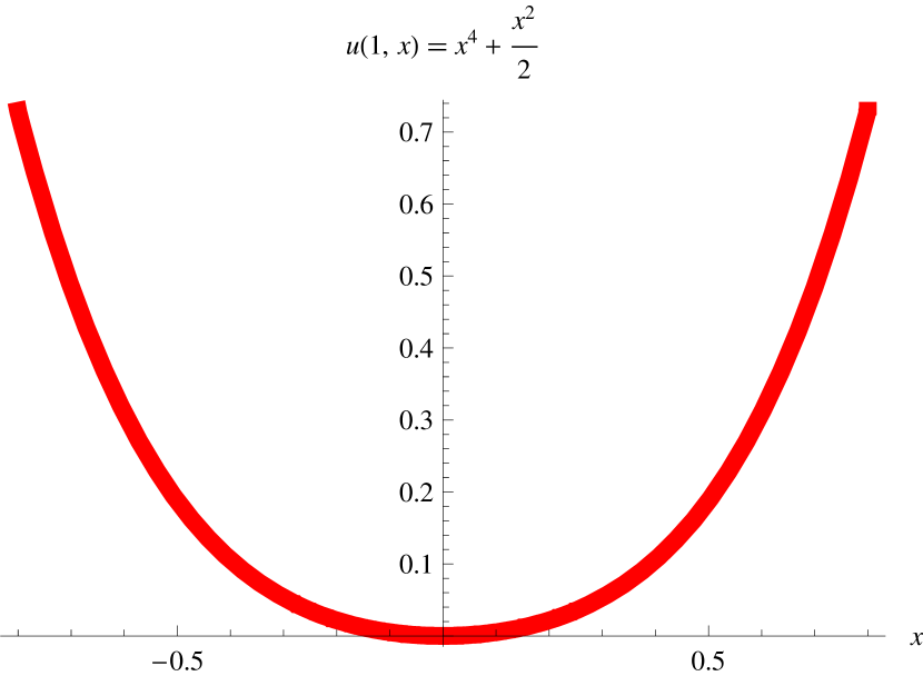
(a)

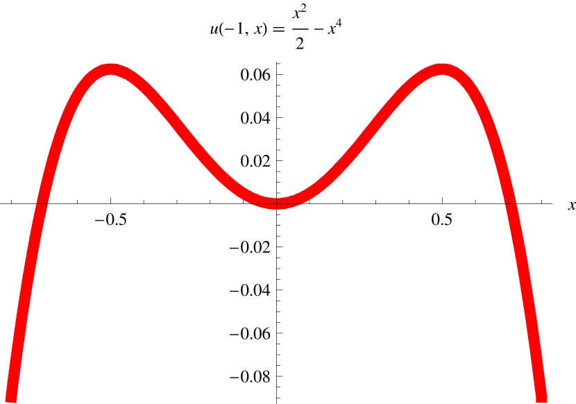
(b)

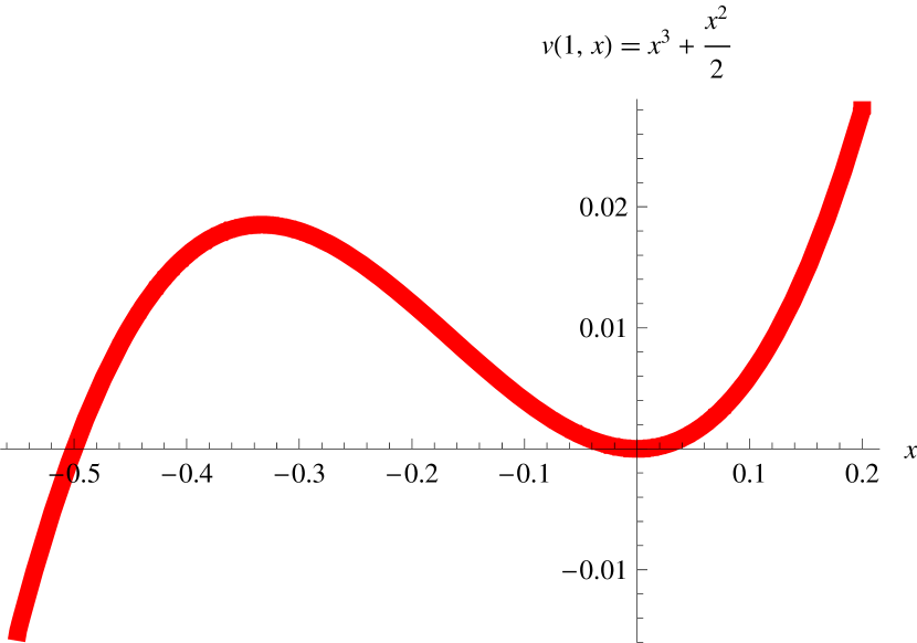
(c)

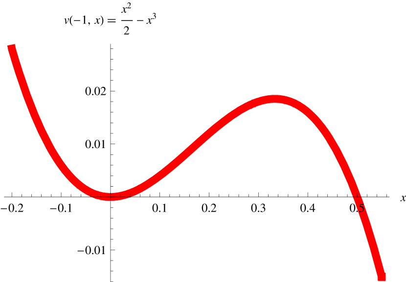
(d)

Figure 1: Plot of the potentials $u(\gamma,x)=\tfrac{1}{2}x^{2}+\gamma x^{4}$ and $v(\gamma,x)=\tfrac{1}{2}x^{2}+\gamma x^{3}$ for positive and negative coupling $\gamma=\pm 1$.

For the quartic potential and positive coupling $\gamma>0$, the spectrum of the Hamiltonian $-\frac{1}{2}\partial_{x}^{2}+u(\gamma>0,x)$, endowed with $L^{2}$ boundary conditions, consists of discrete energy levels which represent physically stable states with zero decay width. For $\gamma<0$, the potential $u(\gamma,x)$ has a double-hump structure, and the particle can escape either to the left or to the right of the “middle valley” by tunneling (see Figs. 1(a) and 1(b)). So, when we change the sign of the coupling parameter, then “the physics of the potential changes drastically.” We can then use the fact that, as a function of $\gamma$, the energy eigenvalues of the quartic oscillator have a branch cut along the negative real axis [2, 3, 4] and write a dispersion relation. It has been stressed in [23, 24] that the discontinuity of the energy levels is given exactly by the instanton configuration, and this fact has been widely used in the literature in the analysis of related problems in quantum physics and field theory.

(Actually, when acting on $L^{2}$, the negative-coupling quartic potential still possesses a real spectrum with discrete eigenvalues, but the analysis is highly nontrivial [25]. Indeed, the natural eigenenergies that are obtained from the real energies for positive coupling by analytic continuation as the complex argument of coupling parameter and of the boundary conditions, are just the complex resonance energies for which the dispersion relation holds.)

Now let us investigate the odd potential $v(\gamma,x)=x^{2}/2+\gamma x^{3}$. When $\gamma$ here changes sign, the physics of the potential does not change (see Figs. 1(c) and 1(d)): still, the particle can escape the “middle valley” by tunneling. Resonances occur. The question is whether we now have two branch cuts as a function of $\gamma$, one along the positive-$\gamma$ axis and one for negative $\gamma$. Should we attempt to formulate a dispersion with integration along $\gamma\in(-\infty,0)$ and $\gamma\in(0,\infty)$? The answer is no. Rather, we should redefine the coupling in such a way that the $\mathcal{PT}$-symmetry of the potential is used effectively. This means that the spectrum is real for purely imaginary coupling $\gamma=\mathrm{i}\,\beta$ with real $\beta$, and it is invariant under the transformation $\gamma=\mathrm{i}\,\beta\to\gamma=-\mathrm{i}\,\beta$. In some sense, the case of the cubic potential for purely imaginary coupling is equivalent to the quartic potential for positive coupling parameter, and the case of the cubic potential for positive coupling is equivalent to the quartic potential for negative coupling parameter. The key thus is to formulate the energy levels of the cubic as a function of $g=\gamma^{2}$, not $\gamma$ itself [19].

3 Some results

We here summarize a few results obtained recently [22] regarding the higher-order corrections for the energy levels of general even-order and odd-order anharmonic oscillators, using the quartic and cubic potentials as examples. Let us thus consider the two Hamiltonians,

$$H(g)=-\frac{1}{2}\frac{\partial^{2}}{\partial x^{2}}+U(g,x),\qquad U(g,x)=\frac{1}{2}x^{2}+gx^{4},$$

$$h(g)=-\frac{1}{2}\frac{\partial^{2}}{\partial x^{2}}+V(g,x),\qquad V(g,x)=\frac{1}{2}x^{2}+\sqrt{g}x^{3},$$

in the unstable region, i.e. for $g<0$ in the quartic case, and for $g>0$ in the cubic case. We assume both Hamiltonians to be endowed with boundary conditions for the resonance energies (which leads to a nonvanishing negative imaginary part for the resonance energy eigenvalues). Specifically, we denote the resonance eigenenergies by $E_{n}(g)$ for the quartic and $\epsilon_{n}(g)$ for the cubic, respectively. The quartic potential is plotted in the range $g\in(-2,-\tfrac{1}{2})$ in Fig. 2(a), and the cubic potential is plotted in the range $g\in(\tfrac{1}{2},2)$ in Fig. 2(b).

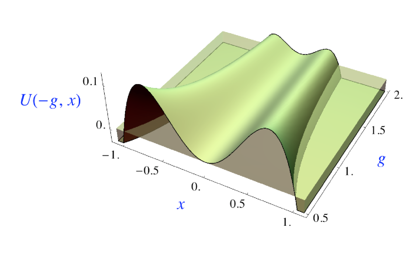
(a)

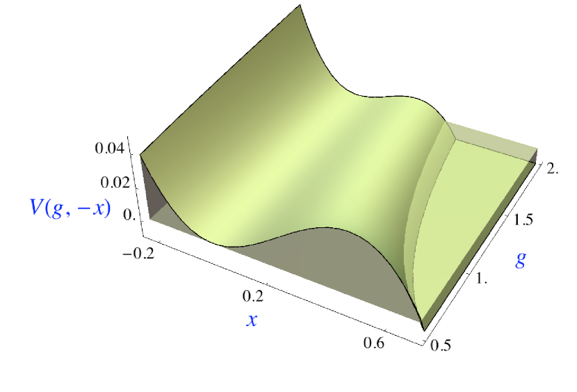
(b)

Figure 2: (a) The quartic potential $U(g,x)=\frac{1}{2}x^{2}+gx^{4}$ is plotted in the parameter range $g\in(-2.0,-0.5)$. As a function of the coupling $g$, the distance that the quantal particle has to tunnel before it escapes from the middle valley decreases as the coupling parameter increases. The decay width of the ground state is proportional to $\exp[1/(3g)]$ (for $g<0$) and increases with the coupling. Higher-order corrections to this well-known result are indicated here (see equation (5)). (b) The cubic potential $V(g,x)=\frac{1}{2}x^{2}+\sqrt{g}x^{3}$ is plotted in the parameter range $g\in(0.5,2.0)$. The decay width of the ground state is proportional to $\exp[-2/(15g)]$ and increases with the coupling.

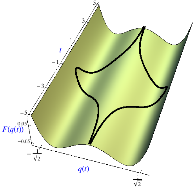
(a)

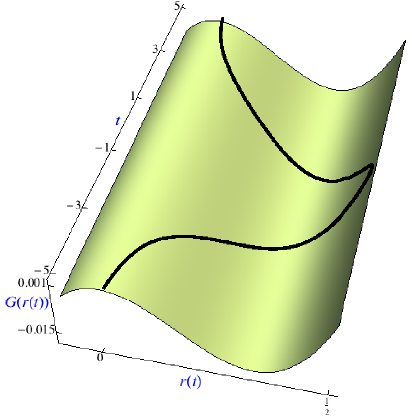
(b)

Figure 3: (a) Quartic instanton. (b) Cubic instanton. See also equations (1) and (2).

Let us now investigate the instanton actions (see also Fig. 3). We write the classical Euclidean actions for the quartic and cubic, respectively, as

$$S[x]=\int\mathrm{d}t\left(\tfrac{1}{2}\dot{x}^{2}+\tfrac{1}{2}x^{2}+g\,x^{4}\right),\qquad s[y]=\int\mathrm{d}t\left(\tfrac{1}{2}\dot{y}^{2}+\tfrac{1}{2}y^{2}+\sqrt{g}y^{3}\right),$$

and perform the following scale transformation $x\equiv x(t)=(-g)^{-1/2}\,q(t)$ and $y\equiv y(t)=-g^{-1/2}\,r(t)$ to arrive at

$$S[q]=-\frac{1}{g}\int\mathrm{d}t\left(\tfrac{1}{2}\dot{q}^{2}+\tfrac{1}{2}q^{2}-q^{4}\right),\qquad s[r]=\frac{1}{g}\int\mathrm{d}t\left(\tfrac{1}{2}\dot{r}^{2}+\tfrac{1}{2}r^{2}-r^{3}\right).$$

Indeed, the width of the resonance is proportional to the exponential of minus the Euclidean action of the instanton configuration, which in turn is a solution to the classical equations of motion in the “inverted” potentials $F(q)=q^{4}-\tfrac{1}{2}q^{2}$ and $G(r)=r^{3}-\tfrac{1}{2}r^{2}$. The instanton is given in Fig. 3. The instanton solutions read

$$q(t)=q_{\mathrm{cl}}(t)=\pm\left[\cosh(2t)+1\right]^{-1/2}$$ (1)

for the quartic and

$$r(t)=r_{\mathrm{cl}}(t)=\left[\cosh(t)+1\right]^{-1}$$ (2)

for the cubic potential. Evaluating the instanton action, one obtains the leading-order results,

$$S[q_{\mathrm{cl}}]=-\frac{1}{3g},\qquad s[r_{\mathrm{cl}}]=\frac{2}{15g}.$$

Observe that both instanton actions are positive in the relevant regions, where the potential is unstable ($g<0$ and $g>0$, respectively). Consequently, the decay widths of the resonances of the quartic and cubic potential are proportional to $\exp[1/(3g)]$ and $\exp[-2/(15g)]$, respectively.

In order to evaluate higher-order corrections are general formulas for oscillators of arbitrary degree, one needs dispersion relations. These reads for the quartic and the cubic, respectively,

$$E_{n}(g)=n+\frac{1}{2}-\frac{g}{\pi}\int_{-\infty}^{0}\mathrm{d}s\ \frac{{\rm Im}\,E_{n}(s+{\rm i}\,0)}{s(s-g)},$$ (3a)

and [19]

$$\epsilon_{n}(g)=n+\frac{1}{2}+\frac{g}{\pi}\int_{0}^{\infty}\mathrm{d}s\frac{{\rm Im}\,\epsilon_{n}^{(M)}(s+{\rm i}\,0)}{s(s-g)}.$$ (3b)

One might ask if the integration for the cubic really stretches to $s=+\infty$. The answer is affirmative: according to [26], we may write the leading terms for the complex strong-coupling expansion for the first three resonances of the cubic as

$$\epsilon_{0}(g+{\rm i}\,0)\;\mathop{=}^{g\to\infty}\;g^{1/5}\,0.762851775\,\mathrm{e}^{-\mathrm{i}\,\pi/5},$$

$$\epsilon_{1}(g+{\rm i}\,0)\;\mathop{=}^{g\to\infty}\;g^{1/5}\,2.711079923\,\mathrm{e}^{-\mathrm{i}\,\pi/5},$$

$$\epsilon_{2}(g+{\rm i}\,0)\;\mathop{=}^{g\to\infty}\;g^{1/5}\,4.989240088\,\mathrm{e}^{-\mathrm{i}\,\pi/5}.$$

Here, we choose boundary conditions for the wave functions such as to generate resonance energies with a negative imaginary part, which are relevant for the dispersion integral (3b) as they are “attached” to values of the coupling with an infinitesimal positive imaginary part. Intuitively, we might assume that at least the second and the third resonance might disappear for very strong coupling $g$. This is because the classically forbidden region of the cubic potential which separates the fall-off region from the “middle valley” becomes smaller and smaller as the coupling increases, and indeed, the second excited level lies well above the relevant energy region in which tunneling would be necessary (see also Fig. 2(b)). However, this point of view does not hold: the resonance persists for arbitrarily large coupling, and the physical picture is that the “escape” of the probability density to infinity, which for the cubic happens in finite time, provides for a sufficient mechanism to induce a nonvanishing decay width of the resonance, even if the traditional tunneling picture is not applicable (similar considerations apply to the resonances in the Stark effect [27]). These considerations can be generalized to odd potentials of arbitrary order, and to arbitrary excited levels [22]. One result stemming from this generalization is given in the Appendix.

Using generalized Bohr–Sommerfeld quantizations which are inspired by the treatment of double-well-like potentials [15, 16], one can formulate a general formalism [22] which allows to write down higher-order formulas for the complex resonance energies. In contrast to [22], where we focused on the first few correction terms for the anharmonic oscillators of the third, sixth and seventh degree, here we would like to fully concentrate on the cubic and quartic oscillators and indicate the generalized nonanalytic expansion exclusively for the oscillators of the third and the forth degree. Specifically, we have for a resonance of the quartic,

$$E_{n}(g<0)=\sum_{K=0}^{\infty}E_{n,K}\,g^{K}$$

$$\phantom{E_{n}(g<0)=}{}+\sum_{J=1}^{\infty}\left[\frac{\mathrm{i}}{\sqrt{\pi}\,n!}\frac{2^{2n+\frac{1}{2}}}{(-g)^{n+\frac{1}{2}}}\exp\left(-\frac{1}{3g}\right)\right]^{J}\sum_{L=0}^{J-1}\,\ln^{L}\left(\frac{4}{g}\right)\sum_{K=0}^{\infty}\Xi^{(4,n)}_{J,L,K}g^{K}$$ (4a)

and for a general resonance of the cubic,

$$\epsilon_{n}(g>0)=\sum_{K=0}^{\infty}\epsilon_{n,K}\,g^{K}$$

$$\phantom{\epsilon_{n}(g>0)=}{}+\sum_{J=1}^{\infty}\left[\frac{\mathrm{i}}{\sqrt{\pi}\,n!}\frac{2^{3n}}{g^{n+\frac{1}{2}}}\exp\left(-\frac{2}{15g}\right)\right]^{J}\sum_{L=0}^{J-1}\ln^{L}\left(-\frac{8}{g}\right)\sum_{K=0}^{\infty}\Xi^{(3,n)}_{J,L,K}g^{K},$$ (4b)

where the $\Xi$ are constant coefficients. (In contrast to [22], we here single out the perturbative contributions $\sum_{K=0}^{\infty}E_{n,K}g^{K}$ and $\sum_{K=0}^{\infty}\epsilon_{n,K}g^{K}$ from the instanton effects, which are given by the terms with $J=1,\ldots,\infty$.)

Of particular phenomenological relevance is the term with $J=1$ as it contains the perturbative corrections about the instanton configuration and is very important for comparison with numerically determined resonance eigenenergies of the systems. Without details, we only quote here [22] the results for the higher-order corrections to the ground state and to the first excited state of the quartic, which read

$${\rm Im}\,E_{0}(g<0)=-\exp\left(\frac{1}{3\,g}\right)\sqrt{-\frac{2}{\pi g}}\left\{1+\frac{95}{24}g-\frac{13259}{1152}g^{2}+\frac{8956043}{82944}g^{3}\right.$$

$$\hphantom{{\rm Im}\,E_{0}(g<0)=}{}-\frac{11481557783}{7962624}g^{4}+\frac{4580883830443}{191102976}g^{5}-\frac{12914334973382407}{27518828544}g^{6}$$ (5a)

$$\left.\hphantom{{\rm Im}\,E_{0}(g<0)=}{}+\frac{6938216714164463905}{660451885056}g^{7}-\frac{33483882026182043052421}{126806761930752}g^{8}+{\mathcal{O}}(g^{9})\right\}$$

and

$${\rm Im}\,E_{1}(g<0)=-\exp\left(\frac{1}{3\,g}\right)\sqrt{-\frac{32}{\pi g^{3}}}\left\{1+\frac{371}{24}g-\frac{3371}{1152}g^{2}+\frac{33467903}{82944}g^{3}\right.$$

$$\phantom{{\rm Im}\,E_{1}(g<0)=}{}-\frac{73699079735}{7962624}g^{4}+\frac{44874270156367}{191102976}g^{5}-\frac{181465701024056263}{27518828544}g^{6}$$ (5b)

$$\left.\phantom{{\rm Im}\,E_{1}(g<0)=}{}+\frac{133606590325852428349}{660451885056}g^{7}-\frac{850916613482026035123397}{126806761930752}g^{8}+{\mathcal{O}}(g^{9})\right\},$$

and for the lowest two levels of the cubic, which are

$${\rm Im}\,\epsilon_{0}(g>0)=-\frac{\exp\left(-\frac{2}{15\,g}\right)}{\sqrt{\pi g}}\left\{1-\frac{169}{16}g-\frac{44507}{512}g^{2}-\frac{86071851}{40960}g^{3}-\frac{189244716209}{2621440}g^{4}\right.$$

$$\phantom{{\rm Im}\,\epsilon_{0}(g>0)=}{}-\frac{128830328039451}{41943040}g^{5}-\frac{1027625748709963623}{6710886400}g^{6}$$ (6a)

$$\left.\phantom{{\rm Im}\,\epsilon_{0}(g>0)=}{}-\frac{933142404651555165943}{107374182400}g^{7}-\frac{7583898146256325425743381}{13743895347200}g^{8}+{\mathcal{O}}(g^{9})\right\}$$

and

$${\rm Im}\,\epsilon_{1}(g>0)=-\frac{8\exp\left(-\frac{2}{15g}\right)}{\sqrt{\pi}g^{3/2}}\left\{1-\frac{853}{16}g+\frac{33349}{512}g^{2}-\frac{395368511}{40960}g^{3}\right.$$

$$\phantom{{\rm Im}\,\epsilon_{1}(g>0)=}{}-\frac{1788829864593}{2621440}g^{4}-\frac{2121533029723423}{41943040}g^{5}$$

$$\phantom{{\rm Im}\,\epsilon_{1}(g>0)=}{}-\frac{27231734458812207783}{6710886400}g^{6}-\frac{37583589061337851179291}{107374182400}g^{7}$$

$$\left.\phantom{{\rm Im}\,\epsilon_{1}(g>0)=}{}-\frac{442771791224240926548268373}{13743895347200}g^{8}+{\mathcal{O}}(g^{9})\right\}.$$ (6b)

Note that the higher-order terms for the ground state of the cubic, by virtue of the dispersion relation (3b), are in full agreement with the higher-order formulas given in [19]. Note also that both above results for the ground state could have been found by plain perturbation theory about the instanton configuration, but the results for the excited states are somewhat less trivial to obtain; they follow from the general formalism outlined in [22].

4 Conclusions

Our generalized nonanalytic expansions (4a) and (4b) provide for an accurate description of resonance energies of the quartic and cubic anharmonic oscillators. These combine exponential factors, logarithms and power series in a systematic, but highly nonanalytic formula. Note that the term “resurgent functions” has been used in the mathematical literature [28, 29, 30] in order to describe such mathematical structures; we here attempt to denote them using a more descriptive, alternative name.

In a general context, we conclude that a physical phenomenon sometimes cannot be described by a power series alone. We have to combine more than one functional form in order to write down a systematic, but not necessarily analytic expansion in order to describe the phenomenon in question. In the context of odd anharmonic oscillators, the generalized nonanalytic expansions which describe the energy levels in higher orders are intimately connected to the dispersion relations (3a) and (3b) which in turn profit from the $\mathcal{PT}$-symmetry of the odd anharmonic oscillators for purely imaginary coupling. The $\mathcal{PT}$-symmetry is used here as an indispensable, auxiliary device in our analysis (it is perhaps interesting to note that the use of $\mathcal{PT}$-symmetry as an auxiliary device has recently helpful in a completely different context [31]). In our case, very large coefficients are obtained for, e.g., the perturbation about the instanton for the first excited state of the cubic (see equation (6b)). At a coupling of $g=0.01$, the first correction term $-853g/16$ halves the result for the decay width of the first excited state, and the higher-order terms are equally important.

We have recently generalized the above treatment to higher-order corrections to anharmonic oscillators up to the tenth order. The oscillators of degree six and seven display very peculiar properties: for the sixth degree, some of the correction terms accidentally cancel, and for the septic potential, the corrections can be expressed in a natural way in terms of the golden ratio $\phi=(\sqrt{5}+1)/2$. For the potential of the seventh degree, details are discussed in [22].

Let us conclude this article with two remarks regarding the necessity of using general non-analytic expansions to describe physical phenomena. First, the occurrence of the nonanalytic exponential terms is connected with the presence of branch cuts relevant to the description of physical quantities as a function of the coupling, as exemplified by the equations (3a) and (3b). Second, the presence of higher-order terms in the generalized expansions is due to our inability to solve the eigenvalue equations exactly, or, in other words, to carry out WKB expansions in closed form to arbitrarily high order. These two facts, intertwined, give rise to the mathematical structures that we find here in equations (4a) and (4b).

Appendix

Using the dispersion relation (3b) and a generalization of the instanton configuration (2) to arbitrary odd oscillators, one may evaluate the decay width for a general state of an odd potential and general large-order (“Bender–Wu”) formulas for the large-order behavior of the perturbative coefficients of arbitrary excited levels for odd anharmonic oscillators. For a general perturbation of the form $\sqrt{g}\,x^{M}$, with odd $M\geq 3$, with resonance energies $\epsilon^{(M)}_{n}(g)\sim\sum_{K}\epsilon^{(M)}_{n,K}g^{K}$, we obtain [22] in the limit $K\to\infty$,

$$\epsilon^{(M)}_{n,K}\;\sim\;-\frac{(M-2)\Gamma\left((M-2)K+n+\tfrac{1}{2}\right)}{\pi^{3/2}n!2^{2K+1-n}}\left[B\left(\frac{M}{M-2},\frac{M}{M-2}\right)\right]^{-(M-2)K-n-\tfrac{1}{2}},$$

where $B(x,y)=\Gamma(x)\Gamma(y)/\Gamma(x+y)$ is the Euler Beta function.

Acknowledgments

U.D.J. acknowledges helpful conversations with C.M. Bender and J. Feinberg at PHHQP2008 at the conference venue in Benasque (Spain). A.S. acknowledges support from the Helmholtz Gemeinschaft (Nachwuchsgruppe VH–NG–421).

References

- [1]
- [2] Bender C.M., Wu T.T., Anharmonic oscillator, Phys. Rev. 184 (1969), 1231–1260.
- [3] Bender C.M., Wu T.T., Large-order behavior of perturbation theory, Phys. Rev. Lett. 27 (1971), 461–465.
- [4] Bender C.M., Wu T.T., Anharmonic oscillator. II. A study in perturbation theory in large order, Phys. Rev. D 7 (1973), 1620–1636.
- [5] Le Guillou J.C., Zinn-Justin J., Critical exponents for the -vector model in three dimensions from field theory, Phys. Rev. Lett. 39 (1977), 95–98.
- [6] Le Guillou J.C., Zinn-Justin J., Critical exponents from field theory, Phys. Rev. B 21 (1980), 3976–3998.
- [7] Itzykson C., Zuber J.B., Quantum field theory, McGraw-Hill, New York, 1980.
- [8] Pachucki K., Effective Hamiltonian approach to the bound state: Positronium hyperfine structure, Phys. Rev. A 56 (1997), 297–304.
- [9] Erickson G.W., Yennie D.R., Radiative level shifts. I. Formulation and lowest order Lamb shift, Ann. Physics 35 (1965), 271–313.
- [10] Erickson G.W., Yennie D.R., Radiative level shifts. II. Higher order contributions to the Lamb shift, Ann. Physics 35 (1965), 447–510.
- [11] Karshenboim S.G., Two-loop logarithmic corrections in the hydrogen Lamb shift, J. Phys. B 29 (1996), L29–L31.
- [12] Pachucki K., Logarithmic two-loop corrections to the Lamb shift in hydrogen, Phys. Rev. A 63 (2001), 042503, 8 pages, physics/0011044.
- [13] Jentschura U.D., Pachucki K., Two-loop self-energy corrections to the fine structure, J. Phys. A: Math. Gen. 35 (2002), 1927–1942, hep-ph/0111084.
- [14] Oppenheimer J.R., Three notes on the quantum theory of aperiodic fields, Phys. Rev. 31 (1928), 66–81.
- [15] Zinn-Justin J., Jentschura U. D., Multi-instantons and exact results. I. Conjectures, WKB expansions, and instanton interactions, Ann. Physics 313 (2004), 197–267, quant-ph/0501136.
- [16] Zinn-Justin J., Jentschura U.D., Multi-instantons and exact results. II. Specific cases, higher-order effects, and numerical calculations, Ann. Physics 313 (2004), 269–325, quant-ph/0501137.
- [17] Jentschura U.D., Zinn-Justin J., Instanton in quantum mechanics and resurgent expansions, Phys. Lett. B 596 (2004), 138–144, hep-ph/0405279.
- [18] Bender C.M., Boettcher S., Real spectra in non-Hermitian Hamiltonians having -symmetry, Phys. Rev. Lett. 80 (1998), 5243–5246, physics/9712001.
- [19] Bender C.M., Dunne G.V., Large-order perturbation theory for a non-Hermitian -symmetric Hamiltonian, J. Math. Phys. 40 (1999), 4616–4621, quant-ph/9812039.
- [20] Bender C.M., Boettcher S., Meisinger P.N., -symmetric quantum mechanics, J. Math. Phys. 40 (1999), 2201–2229, quant-ph/9809072.
- [21] Bender C.M., Brody D.C., Jones H.F., Complex extension of quantum mechanics, Phys. Rev. Lett. 89 (2002), 270401, 4 pages, Erratum, Phys. Rev. Lett. 92 (2004), 119902, quant-ph/0208076.
- [22] Jentschura U.D., Surzhykov A., Zinn-Justin J., Unified treatment of even and odd anharmonic oscillators of arbitrary degree, Phys. Rev. Lett. 102 (2009), 011601, 4 pages.
- [23] Zinn-Justin J., Quantum field theory and critical phenomena, 3rd ed., Clarendon Press, Oxford, 1996.
- [24] Zinn-Justin J., Intégrale de chemin en mécanique quantique: Introduction, CNRS Éditions, Paris, 2003.
- [25] Feinberg J., Peleg Y., Self-adjoint Wheeler–DeWitt operators, the problem of time, and the wave function of the Universe, Phys. Rev. D 52 (1995), 1988–2000, hep-th/9503073.
- [26] Jentschura U.D., Surzhykov A., Lubasch M., Zinn-Justin J., Structure, time propagation and dissipative terms for resonances, J. Phys. A: Math. Theor. 41 (2008), 095302, 16 pages, arXiv:0711.1073.
- [27] Benassi L., Grecchi V., Harrell E., Simon B., Bender–Wu formula and the Stark effect in hydrogen, Phys. Rev. Lett. 42 (1979), 704–707, Erratum, Phys. Rev. Lett. 42 (1979), 1430.
- [28] Pham F., Fonctions résurgentes implicites, C. R. Acad. Sci. Paris Sér. I Math. 309 (1989), no. 20, 999–1004.
- [29] Delabaere E., Dillinger H., Pham F., Développements semi-classiques exacts des niveaux d’énergie d’un oscillateur à une dimension, C. R. Acad. Sci. Paris Sér. I Math. 310 (1990), no. 4, 141–146.
- [30] Candelpergher B., Nosmas J.C., Pham F., Approche de la Résurgence, Hermann, Paris, 1993.
- [31] Andrianov A.A., Cannata F., Giacconi P., Kamenshchik A.Y., Regoli D., Two-field cosmological models and large-scale cosmic magnetic fields, J. Cosmol. Astropart. Phys. 2008 (2008), no. 10, 019, 12 pages, arXiv:0806.1844.