The complex polarization angles of radio pulsars: orthogonal jumps and interstellar scattering

Abstract

Despite some success in explaining the observed polarisation angle swing of radio pulsars within the geometric rotating vector model, many deviations from the expected S-like swing are observed. In this paper we provide a simple and credible explanation of these variations based on a combination of the rotating vector model, intrinsic orthogonally polarized propagation modes within the pulsar magnetosphere and the effects of interstellar scattering. We use simulations to explore the range of phenomena that may arise from this combination, and briefly discuss the possibilities of determining the parameters of scattering in an effort to understand the intrinsic pulsar polarization.

1 Introduction

Polarization properties of radio pulsars which are observed in many sources should form the basis of any attempted interpretation. First of all, the degree of polarization in pulsars is generally high: often over 50% in its linear component (hereafter L) and 10-15% in its circular component (hereafter V) (e.g. Gould & Lyne 1998). Linear polarization decreases with observing frequency, and is generally low above a few GHz. An exception to this rule is found in young pulsars with a large spin down energy derivative $\rm{\dot{E}}$, which remain highly polarized up to frequencies above 5 GHz (von Hoensbroech et al. 1998, Weltevrede & Johnston 2008 in prep.).

In some pulsars, the polarization position angle (hereafter PA), swings in a smooth way across the pulse profile. The smoothness of the PA swing lends support to the single rotating vector model of Radhakrishnan & Cooke (1969), whereby the angle of polarization is tied to the magnetic field lines, and changes gradually as the line-of-sight intersects different field lines at different angles, as:

$$\tan{(PA-PA_{0})}=\frac{\sin({\phi-\phi_{0}})\sin{\alpha}}{\sin{\zeta}\cos{\alpha}-\cos{\zeta}\sin{\alpha}\cos{\phi}}$$ (1)

PA₀ and $\phi_{0}$ are constant offsets in PA and phase, $\phi$ the pulse phase, $\alpha$ the inclination angle between magnetic and rotation axis, and $\zeta$ the sum of $\alpha$ and the impact parameter $\beta$. This equation is derived with the convention that the position angle increases clockwise on the sky. This purely geometric model has been used to derive the geometry of a number of pulsars where fitting of PA data is possible (e.g. Everett & Weisberg 2001). However, kinks, wiggles and jumps of various magnitudes often occur in observed PA swings (recent examples can be found in Johnston et al. 2008). Figure 1 shows the well-known bright pulsar PSR B0355+54 at 1.4 GHz; the data are from Gould & Lyne (1998). The PA swing shows an abrupt orthogonal jump at pulse phase 0.02, and a bump-like feature at pulse phase 0.05, superposed on a gradual, S-shaped swing.

In addition, and contradictory to the predictions of the geometric model, PA swings have been observed not to be entirely frequency independent (e.g. Karastergiou & Johnston 2006). One known reason for this is that orthogonal polarization modes have been observed to have different spectral indices (Karastergiou et al. 2005, Smits et al. 2006), and therefore orthogonal jumps in the PA swing appear at different locations within the pulse at different frequencies. A second known frequency dependence of PA swings is caused by interstellar scattering. Li & Han (2003) demonstrated that it is possible to explain low frequency PA swings by convolving the Stokes profiles of high frequency data with appropriate scattering functions. They show how scattering flattens the S-shaped PA curve of the rotating vector model, rendering the derived geometrical parameters from fitting erroneous. This was recently also shown for PSR J0908-4913 by Kramer & Johnston (2008), who demonstrated that the PA swing is indeed independent of frequency if scattering is taken into account.

In this paper, we investigate how observed PA swings like the example of Figure 1 can result from simple intrinsic PA swings, orthogonal polarization mode jumps and small amounts of scattering. We show with simulations how orthogonal PA jumps can significantly distort the PA swing. We demonstrate the modest magnitude of scattering necessary to explain the observed shapes of PA swings with orthogonal jumps and study other consequences of this unexplored, frequency dependent phenomenon.

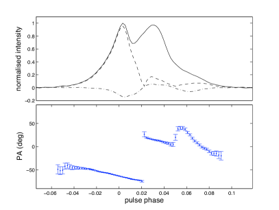
Figure 1: The polarization profile of PSR B0355+54 from Gould & Lyne (1998) at 1.4 GHz. The solid line shows the normalised total power, the dashed line the linear polarization and the dot-dashed line the circular polarization. The issues discussed in this paper are exemplified by the PA in the lower panel, which features an orthogonal and non-orthogonal jump distorting an apparently smooth swing.

2 Description of the numerical simulations

Extensive simulations were carried out to explore scattering effects on polarization pulse profiles. In contrast to Li & Han, we use simulated pulsar data adhering to the rotating vector model for the PA, rather than high frequency profiles. By examining the scattered simulated profiles and comparing them to real pulsar profiles, it is possible to test the effects of interstellar scattering. The software developed for this purpose follows these steps:

1. A realistic average pulse profile is generated out of a small number of Gaussian components, where the PA follows the rotating vector model interrupted only by possible 90$\degr$ jumps.

2. All 4 “intrinsic” Stokes parameters are then convolved with the desired response function $g(t)$ chosen to simulate the effects of scattering and assuming the scattering screen introduces only delays and not rotations in the polarization. We have tested three such functions,

   $$g_{ts}(t)=e^{-\Delta t/\tau_{s}}$$ (2)

   $$g_{ths}(t)=\left(\frac{\pi\tau_{s}}{4t^{3}}\right)^{1/2}\ e^{-\pi^{2}\tau_{s}/16t}$$ (3)

   $$g_{um}(t)=\left(\frac{\pi^{5}\tau_{s}^{3}}{8t^{5}}\right)^{1/2}\ e^{-\pi^{2}\tau_{s}/4t}$$ (4)

   which correspond to the simple case of a thin scattering screen at approximately half way between the source and observer ($g_{ts}$), and the equations of Williamson (1972) for a thick screen near the source ($g_{ths}$) and a uniform medium ($g_{um}$) respectively. For a discussion on the merits and shortcomings of various scattering response functions, see the discussion in Bhat et al. (2003). In all three equations, the scattering constant $\tau_{s}$ is the parameter that determines the magnitude of the effect.

3. The previous step is repeated to simulate an observing backend, with a particular number of frequency channels and channel bandwidth. For each channel, $\tau_{s}$ is computed at the center frequency, by the empirical equation given in Bhat et al. (2004)

   $$log(\tau_{s})=-6.46+0.154*log(DM)+$$

   $$+1.07*log(DM)^{2}-3.86*log(\nu),$$ (5)

   where $\tau_{s}$ is in ms, $DM$ is the dispersion measure in cm³pc and $\nu$ the observing frequency in GHz. Note that observationally there is quite a large scatter in the measured $\tau_{s}$ for a given $DM$. The $DM$ values are chosen to result in small values of $\tau_{s}$, generally comparable to the resolution of the simulated profiles. The exact frequency dependence of $\tau_{s}$ is far from totally certain (e.g. Löhmer et al. 2004). However, the analysis presented in the following does not expand to broad frequency ranges but is confined to typical narrow observing bandwidths: small changes in the frequency exponent, will incur relatively small changes in $\tau_{s}$. A small amount of un-correlated Gaussian noise is added to each of the Stokes profiles to simulate real observational data.

4. The average profile is generated by summing up the simulated frequency channels.

The degree to which a profile is affected by the convolution process depends on the relationship between $\tau_{s}$ and $t_{\rm samp}$, the latter being the temporal resolution of the data. An interesting handle on the process is therefore the ratio between the two, $R=\tau_{s}/t_{\rm samp}$.

3 Simulated and scattered pulse profiles

3.1 Profiles with a single orthogonal PA jump

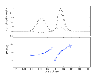
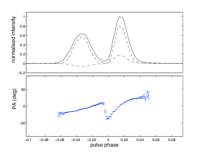
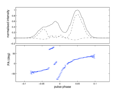
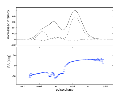
Figure 2: The polarization profile of two simulated pulsars (top and bottom row), as in Figure 1. The unscattered simulated intrinsic data are on the left, and the scattered polarization profiles on the right. The top two plots show a 500 ms period pulsar with one orthogonal mode jump (see discussion in section 3.1), as opposed to a 200 ms pulsar with three orthogonal jumps in the bottom plots (see discussion in section 3.2).

The top two plots of Figure 2 show the input and result of a typical simulation. The period of the simulated pulsar is 500 ms, and the profile consists of 512 bins, resulting in a temporal resolution of $t_{\rm samp}\approx$ 0.976 ms. The “intrinsic” profile is shown on the left. The figure on the right demonstrates the “observed” profile, with a filterbank of 16 16–MHz wide channels, centred at 1.4 GHz, assuming equations 2 and 5. $\tau_{s}$ ranges between $\sim$2.4 and $\sim$1.25 ms in the band, based on an assumed value of 340 cm³pc for the $DM$. The total power profile (solid line) shows no obvious signs of scattering. The most obvious consequence of scattering can be seen in the PA, where the precisely orthogonal jump has flattened out into a more gradual change of not more that $50\degr$ similar to the real data in Figure 1. This feature in the PA swing is very common in real data, and has been a thorn in the side of the model of orthogonal polarization modes. By applying equation 3, a much more modest $\tau_{s}$ of order under 1 ms is sufficient to distort the PA curve in a similar fashion, whereas equation 4 yields similar results to Figure 2 with similar $\tau_{s}$ values. The degree of linear (dashed line) and circular (dot-dashed line) polarization remain largely unaffected by this small amount of scattering.

3.2 Profiles with multiple orthogonal PA jumps

The bottom two plots of Figure 2 show another example of a simulated pulse profile. The pulse period is 200 ms and $t_{\rm samp}\approx$0.39 ms. The “intrinsic” simulated profile has 3 orthogonal PA jumps, which occur in quick succession between phases -0.05 and 0. The $\tau_{s}$ used is the same as the previous example, ranging from 2.4 to 1.25 ms in the band. Given the shorter pulse period and the smaller value of $t_{\rm samp}$, the ratio $R$ is larger ranging from $R\approx 6$ for the lowest frequency channel to $R\approx 3$ for the highest frequency channel for the same configuration of filterbank (i.e. 16 16–MHz channels centred on 1.4 GHz). The total power profile does not show evidence of scattering. However, the PA swing diverges significantly from the simple geometric model. The kinks and wiggles in the PA swing on the right are common in real data, and cause severe difficulties both in fitting the PA data to the rotating vector model, and in theoretical treatment of the magnetospheric processes.

Figure 3: The polarization profile of a simulated pulsar with a period of 200 ms, scattered by various values of $\tau_{s}$, ranging from 0 to 8 ms as indicated.

Figure 3 illustrates the way a polarization profile with orthogonal PA jumps is affected by different values of $\tau_{s}$. Again, the profile has a resolution of $t_{\rm samp}\approx$0.39 ms. Large $\tau_{s}$ ($\geq$4 ms) values result in obvious smearing of the total power profile, however the polarization PA is affected significantly from low $\tau_{s}$ values. Note how the steep, middle part of the PA swing, becomes flat at $\tau_{s}=2$ ms.

3.3 Frequency dependence of the position angle

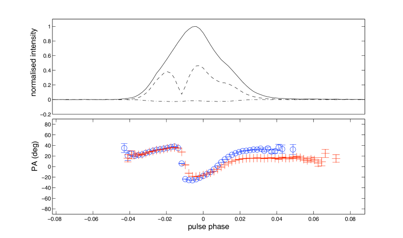
Figure 4: The change in PA across a 256 MHz band at 1.4 GHz. Two PA swings are shown: the crosses correspond to the lowest and the circles to the highest frequency channel. The frequency dependence of $\tau_{s}$ has quite a pronounced effect even at this high observing frequency.

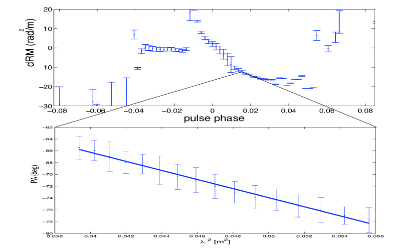
Figure 5: Top: Each bin of the frequency dependent PA swing from Figure 4 has been fitted for a rotation measure in this simulated pulsar, resulting in this phase-resolved rotation measure profile. Bottom: The PA of one bin across 16 frequency channels, plotted versus the wavelength squared. Faraday Rotation would result in a linear dependence, which can be fitted extremely well here with an $RM$ of -13.42 rad/m².

The fact that small amounts of scattering significantly distort the pulsar PA swing, has the direct consequence that observed PA curves are not independent of frequency. This complicates the interpretation of PA swings, especially in comparing data from multiple, widely spaced frequencies. Another consequence of scattering manifests itself within the relatively narrow band of an observation at a given frequency. Figure 4 shows a simulated pulse profile with an orthogonal PA jump and the PA swings of two frequency channels, 256 MHz apart and centred at 1.4 GHz. The circles correspond to the highest and the crosses to the lowest frequency. The PA swings are obviously different, in particular after the pulse phase of the orthogonal jump. This difference will result in slightly different polarization profiles for observations with different bandwidth: for two observations centred on the same frequency, the one with the largest bandwidth will be more affected.

Pulsars are used to determine Faraday Rotation Measures ($RM$) which provide information on the Galactic magnetic field in the direction of the line of sight. $RM$ measurements are based on the assumption that the only frequency dependence of PA arises from Faraday Rotation (taking into account potential orthogonal jumps), which, in the presence of scattering, is not true. A figure showing significant variation in phase resolved $RM$ measurements across the pulse, constitutes the basis of an argument on non-orthogonal modes in pulsar B2016+28 in Ramachandran et al. (2004). The observed Faraday Rotation is an effect of propagation through the interstellar medium and not the pulsar magnetosphere, therefore pulse-phase resolved $RM$ variations are not expected. In that work, an $RM$ is determined for each pulse phase bin, by fitting the simple equation:

$$\Delta PA=RM\frac{c^{2}}{\nu^{2}}$$ (6)

where $c$ the speed of light and $\nu$ the frequency.

We considered interstellar scattering as an alternative explanation to non-orthogonal modes. Simulated scattered data for a band of 16 16–MHz channels at 1.4 GHz were fitted for an $RM$, with no Faraday Rotation included in the simulation. To match the Ramachandran et al. analysis, such a fit was carried out for each pulse phase bin (as shown in the top plot of Figure 5), and although $\tau_{s}$ depends differently on frequency than the PA due to Faraday Rotation, the scattered PAs can be very well fitted by equation 6. The results are shown in Figure 5: in the top panel, the phase resolved fitted $RM$ is shown with errorbars representing the goodness of the fit. It is denoted as $dRM$ on the axis, as it would appear additional to the real interstellar $RM$ of a given source. The bottom panel shows the fit for one phase bin with an apparent negative $RM$ purely due to scattering. The results from these scattering simulations resemble the PSR B2016+28 data, and the PA swing of that pulsar shows evidence of an orthogonal jump (non-orthogonal most likely due to scattering). It is therefore apparent that modest scattering should be considered as an alternative, and in many ways more simple explanation to non-orthogonal modes.

Scattering has implications on the way the $RM$ can be correctly measured. Figure 5 clearly shows that choosing one phase bin, even if it is the most polarized, and fitting for an $RM$ can lead to erroneous results. Similarly, any approach which directly compares PA values of highly polarized bins between channels of different frequencies will also be inaccurate, as demonstrated in Figure 4. The only way to avoid issues pertaining to scattering, is to perform a sum across the profile of the Stokes parameters Q and U for each frequency channel (Noutsos et al. 2008). As scattering only transfers power into (mainly) later pulse phases, it should not affect the sum over the entire profile. The simulations carried out here verify this, and no matter how distorted the phase resolved $RM$ profile, a calculation of $RM$ using the proposed method always yields the $RM$ used for the simulation within the accuracy of the measurement.

4 Discussion

We have shown in the previous section that small amounts of scattering can play an important role in forming the PA swing. We have concentrated on the frequency of 1.4 GHz, as this is where the bulk of observational data lie. In Figures 2 and 3, we have demonstrated the potential of scattering and orthogonal PA jumps to distort the PA swing. Figures 4 and 5 indicate the difficulties this creates on $RM$ measurements. It is obvious from these figures that the phenomenon described here depends critically on the presence and location of orthogonal PA jumps, the degree of scattering and the steepness of the intrinsic PA swing.

As it has been shown in the past and most recently by Kramer & Johnston (2008), in simple PA swings without orthogonal jumps, scattering makes the PA swing flatter. Similarly, if an orthogonal jump is located where the PA is intrinsically flat, scattering cannot create the dramatic kinks and wiggles shown here. The greatest effect is then achieved when orthogonal PA jumps occur near the steepest gradient of the PA swing, as given by equation 1. This is an interesting conclusion, as it is a well established observational fact that the rotating vector model fails predominantly in components nearer to the magnetic axis where the gradient of the PA is steepest (Rankin 1990). A combination of orthogonal PA jumps in this central part of the profile and some scattering, has the potential of generating PA swings only vaguely resembling the simple predicted S-shaped curve. The effect is even further pronounced if orthogonal PA jumps occur in very rapid succession, compared to the scattering constant $\tau_{s}$. If the assumption is made that each emitting patch in the patchy radio beam is in a given polarization mode, a quick succession of jumps near the center of the pulse is an indication that the central components are narrower, as expected if they are emitted at lower altitudes above the pulsar surface (Karastergiou & Johnston 2007).

The combination of a rapidly swinging intrinsic PA, which rapidly jumps by $90\degr$, with scattering can then generate a huge variety of PA swings. As the observed profile is determined by the combination of these effects, a fitting method for the rotation vector model to determine the emission geometry should ideally simultaneously fit for scattering. This will be the object of a more extensive study on this topic, to be presented in the future.

Scattering through the interstellar medium is a stochastic phenomenon, and here we only consider integrated pulse profiles. However, scattering should be similarly responsible for distortions to the polarization of individual pulses. In particular the distributions of single pulse PA values in particular bins are often quoted to be broader than expected by the presence of instrumental noise (e.g. McKinnon 2004, Karastergiou et al. 2002). The next version of scattering simulations will examine the degree to which scattering can reproduce aspects of the observed pulse-to-pulse PA phenomenology.

5 Concluding remarks

We have demonstrated that orthogonal jumps in the PA swings of pulsars, together with very modest amounts of scattering, can lead to distorted PA swings similar to those observed (see Gould & Lyne 1998, Everett & Weisberg 2001 and others for many examples). The natural question that arises is how the effect of scattering can be taken out of the observed data, to recover the intrinsic polarization. Bhat et al. (2003) proposed a scheme, based on the CLEAN algorithm, to attempt this, with considerable success. Attempting this on the full Stokes parameter data seems imperative. Polarization data may impose limitations to the scattering response function and the scattering constant, permitting only orthogonal jumps of PA and an intrinsic PA curve strictly following the rotating vector model in equation 1. This area warrants significant further attention, in an ongoing effort to understand the physics of pulsar radio emission.

References

- Bhat et al. (2004) Bhat N. D. R., Cordes J. M., Camilo F., Nice D. J., Lorimer D. R., 2004, ApJ, 605, 759
- Bhat et al. (2003) Bhat N. D. R., Cordes J. M., Chatterjee S., 2003, ApJ, 584, 782
- Everett & Weisberg (2001) Everett J. E., Weisberg J. M., 2001, ApJ, 553, 341
- Gould & Lyne (1998) Gould D. M., Lyne A. G., 1998, MNRAS, 301, 235
- Johnston et al. (2008) Johnston S., Karastergiou A., Mitra D., Gupta Y., 2008, MNRAS, 388, 261
- Karastergiou & Johnston (2006) Karastergiou A., Johnston S., 2006, MNRAS, 365, 353
- Karastergiou et al. (2005) Karastergiou A., Johnston S., Manchester R. N., 2005, MNRAS, 359, 481
- Karastergiou et al. (2002) Karastergiou A., Kramer M., Johnston S., Lyne A. G., Bhat N. D. R., Gupta Y., 2002, A&A, 391, 247
- Kramer & Johnston (2008) Kramer M., Johnston S., 2008, arXiv, astro-ph 0807.5013v1
- Li & Han (2003) Li X. H., Han J. L., 2003, A&A, 410, 253
- Löhmer et al. (2004) Löhmer O., Mitra D., Gupta Y., Kramer M., Ahuja A., 2004, A&A, 425, 569
- McKinnon (2004) McKinnon M. M., 2004, ApJ, 606, 1154
- Noutsos et al. (2008) Noutsos A., Johnston S., Kramer M., Karastergiou A., 2008, MNRAS, 386, 1881
- Radhakrishnan & Cooke (1969) Radhakrishnan V., Cooke D. J., 1969, Astrophys. Lett., 3, 225
- Ramachandran et al. (2004) Ramachandran R., Backer D. C., Rankin J. M., M. W. J., E. D. K., 2004, ApJ, 606, 1167
- Rankin (1990) Rankin J. M., 1990, ApJ, 352, 247
- Smits et al. (2006) Smits J. M., Stappers B. W., Edwards R. T., Kuijpers J., Ramachandran R., 2006, A&A, 448, 1139
- von Hoensbroech et al. (1998) von Hoensbroech A., Kijak J., Krawczyk A., 1998, A&A, 334, 571
- Weltevrede & Johnston (2008) Weltevrede P., Johnston S., 2008, MNRAS, 387, 1755
- Williamson (1972) Williamson I. P., 1972, MNRAS, 157, 55